Uncertainty-aware demand management of water distribution networks in deregulated energy markets

Abstract

We present an open-source solution for the operational control of drinking water distribution networks which accounts for the inherent uncertainty in water demand and electricity prices in the day-ahead market of a volatile deregulated economy. As increasingly more energy markets adopt this trading scheme, the operation of drinking water networks requires uncertainty-aware control approaches that mitigate the effect of volatility and result in an economic and safe operation of the network that meets the consumers’ need for uninterrupted water supply. We propose the use of scenario-based stochastic model predictive control: an advanced control methodology which comes at a considerable computation cost which is overcome by harnessing the parallelization capabilities of graphics processing units (GPUs) and using a massively parallelizable algorithm based on the accelerated proximal gradient method.

Software availability

Name of software: RapidNet.
Hardware required: CUDA-compliant GPU (tested on NVIDIA Tesla 2075).
Software required: CUDA framework v6.0 or higher (including cuBLAS) and rapidjson (http://rapidjson.org/).
Availability: Open-source software, licence: GNU LGPL v3.0. Available online at https://github.com/GPUEngineering/RapidNet.
Program language: CUDA-C++/C++.
First release: 2017.

1 Introduction

1.1 State of the art

The explosive proliferation of interconnected sensing, computing and communication devices has marked the advent of the concept of cyber-physical systems — ensembles of computational and physical components. In drinking water networks this trend has ushered in new control paradigms where the profusion of data, produced by a network of sensors and stored in a database, is used to prescribe informed control actions [1, 2, 3, 4]. Nevertheless, as these data, be they water demand values or electricity prices, cannot be modeled perfectly, the associated uncertainty is shifted to the decision making process.

The high uncertainty in the operation of drinking water networks, as a result of the volatility of future demands as well as energy prices (in a deregulated energy market) is likely to lead to a rather expensive operating mode with poor quality of service (the network may not always be able to provide the necessary amount of water to the consumers). In control engineering practice, this uncertainty is often addressed in a worst-case fashion [5, 6] — if not neglected at all — leading to conservative and suboptimal control policies. It is evident that it is necessary to devise control methods which take into account the probabilistic nature of the underlying uncertainty making use of the wealth of available historical data aiming at a proactive and foresightful control scheme which leads to an improved closed-loop performance. These requirements necessitate the use of stochastic model predictive control: an advanced control methodology where at every time instant we determine a sequence of control laws which minimizes the expected value of a performance index taken with respect to the distribution of the uncertainty [7]. Optimization-based approaches for the operational management of water networks have been studied and are well established in engineering practice [8].

Indeed, scenario-based stochastic model predictive control (SSMPC) has been shown to lead to remarkable decrease in the operating cost and improvement in the quality of service of drinking water networks [9]. In SSMPC, the uncertain disturbances are treated as random variables on a discrete sample space without assuming any parametric form for their distribution [10]. The scenario approach was identified in a recent review as a powerful method for mitigating uncertainty in environmental modeling related to water management [11]. Although this approach offers a realistic control solution as it is entirely data-driven, this comes with considerable computational burden as the resulting optimization problems are of particularly large scale [12, 13]. This has rendered the use of SSMPC prohibitive and has hindered its applicability. Indeed, hitherto there have been used only conventional model predictive control approaches [14, 15], robust worst-case formulations [5, 16, 17] and stochastic formulations where the underlying uncertainty is assumed to be normally identically independently distributed [18, 19]. Note that it has been observed that demand prediction errors are typically follow heavy-tail distributions which cannot be well approximated by normal ones [20].

In this paper, we present a software for the fast and efficient solution of such problems harnessing the immense computational capabilities of graphics processing units (GPU) building up on our previous work [9, 21, 22].

There has been recently a lot of interest in the development of efficient methods for stochastic optimal control problems such as stochastic gradient methods [23], the alternating directions method of multipliers (ADMM) [24] and various decomposition methods which can lead to parallelizable methods [25, 26] (the most popular being the stochastic dual approximate dynamic programming [27], the progressive hedging approach [28] and dynamic programming [29]). There have been proposed parallelizable interior point algorithms for two-stage stochastic optimal control problems such as [30, 31, 32, 33] and an ad hoc interior point solver for multi-stage problems [34]. However, interior point algorithms involve complex steps and are not suitable for an implementation on GPUs which can make the most of the capabilities of the hardware. Additionally, interior point methods cannot accommodate complex non-quadratic terms in the cost function such as soft constraints (distance-to-set functions).

At large, not many software and libraries are available for stochastic optimal control; one of the very few one may find on the web is JSPD, a generic Java stochastic dynamic programming library. QUASAR is a commercial tool for scenario-based stochastic optimization. One of the most popular tools in the toolbox of the water networks engineer is PLIO [35], which implements MPC algorithms. This work covers the yawning gap between engineering practice and the latest developments in control and optimization theory for drinking water networks. These results can also be applied for the control of other infrastructure with similar structure such as power grids [36].

1.2 Contributions and Novelty

Despite the fact that SSMPC problems typically involve millions of decision variables, the associated optimization problems possess a rich structure which can be exploited to devise parallelizable ad hoc methods to solve the problem more than an order of magnitude faster than commercial solvers running on CPU.

The architecture of our implementation comprises three independent modules: (i) the network module, (ii) the energy prices and water demands forecaster and (iii) the control module. The network module provides a dynamical system model which describes the flow of water across the network together with the storage limits of the tanks and the constraints on pumping capacities. The network module defines a safety storage level for each tank — a level which ensures the availability of water in case of high demand and the maintenance of a minimum required pressure. The forecasters produce a scenario tree, that is, a tree of likely future water demands and energy prices, upon which a contingency plan is made by minimizing a cost function which quantifies the operating cost and the quality of service. Such scenario trees are constructed from historical data of energy prices and water demands. The control module computes flow set-points, which are sent to the pumping stations and valves, by solving a scenario-based stochastic model predictive control problem over a finite prediction horizon.

The proposed stochastic model predictive controller leads to measurable benefits for the operation of the water network. It leads to a more economic operation compared to methods which do not take into consideration the stochastic nature of the energy prices and water demands. In this paper, we assess the performance of the controlled network using three key performance indicators: (i) the economic index, (ii) the safety index, which quantifies the extent of violation of the safety storage level requirement and (iii) the computational complexity index with which we assess the computational feasibility of the controller. Simulation results are provided using data from the water network of Barcelona and the energy market of Austria. The advantages of the adopted control methodology are combined with the computational power of GPUs, which enables us to solve problems of very large scale.

1.3 Software

Our implementation is available as an open-source and free software which can be readily tailored to the needs of different water networks modifying the parameters of its modules. The implementation is done entirely in CUDA-C++ and it can be configured either programmatically or using configuration files. The adopted object-oriented programming model is amenable to extensions and users may specify their own predictive models, scenario trees, cost functions, dynamical models and constraints. Our results are accompanied by extensive benchmarks and the software is verified with unit tests.

2 Modeling

2.1 Hydraulic modeling

The water network involves four types of elements: water tanks, active elements (pumps and valves), mixing nodes and demand sectors. We focus on flow-based water networks where all flows are manipulated variables based on the modeling approaches presented in [37, 14, 38, 13, 5].

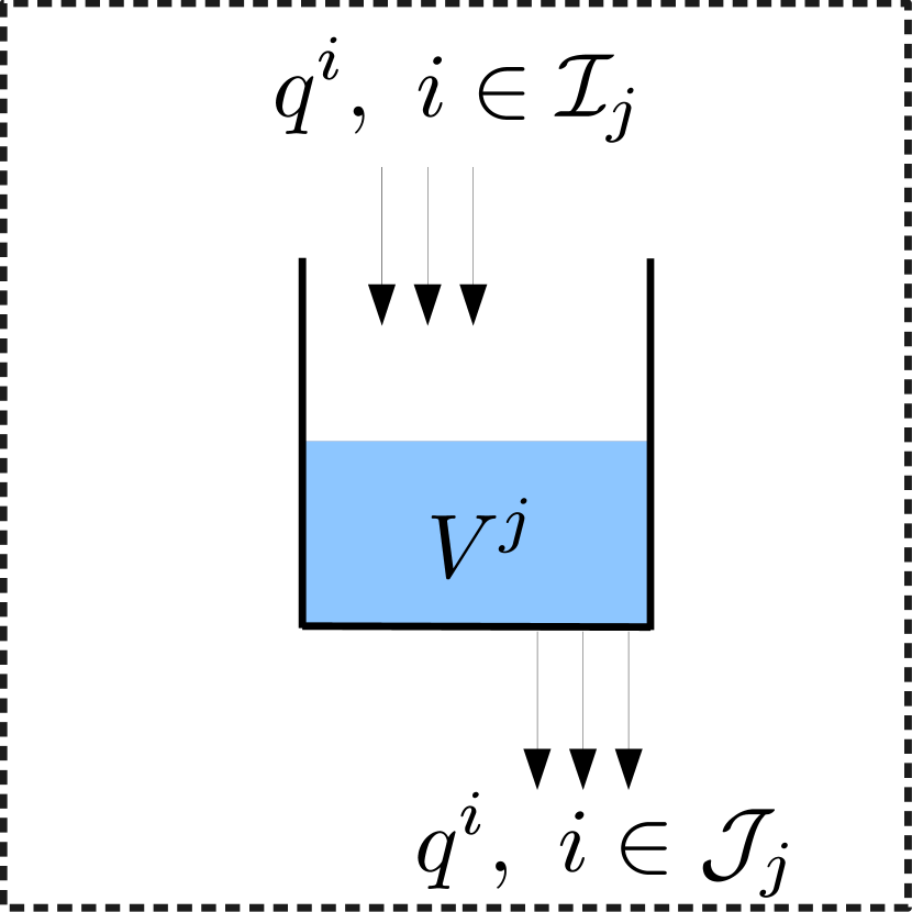
(a) Water tank

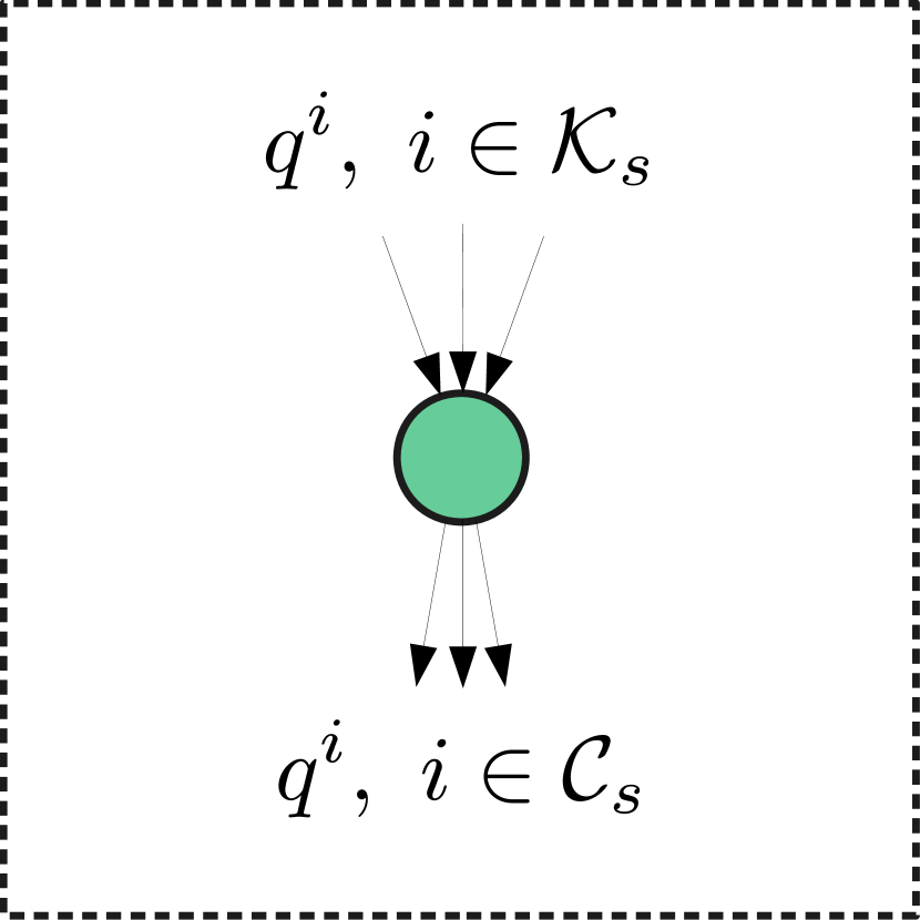
(b) Mixing node

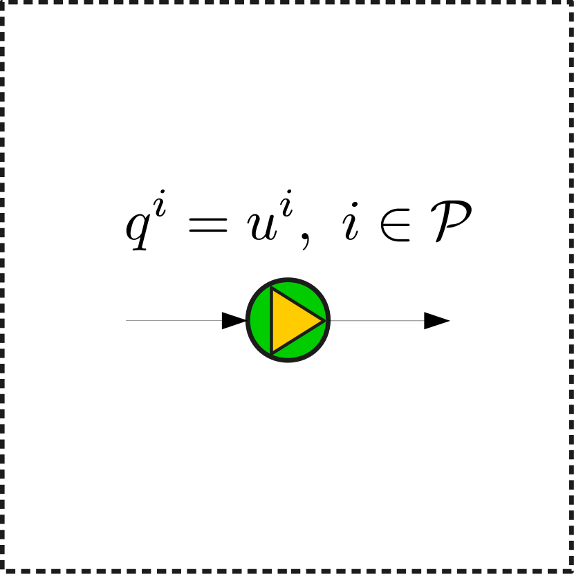
(c) Controlled pump

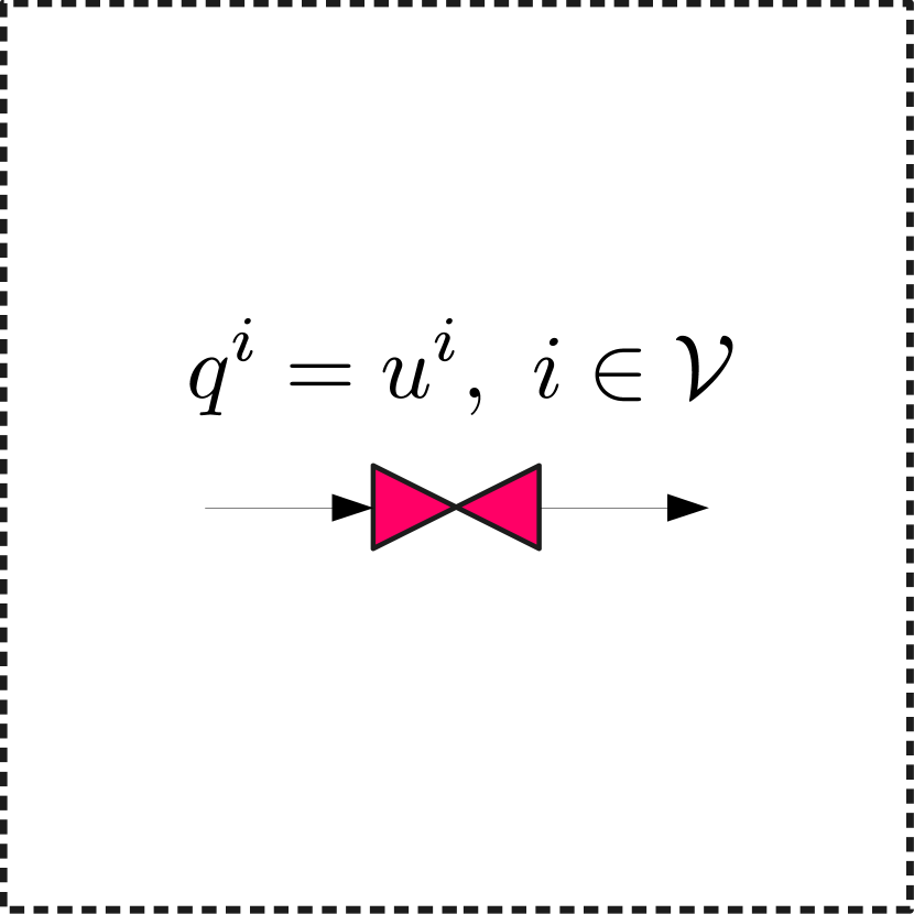
(d) Controlled valve

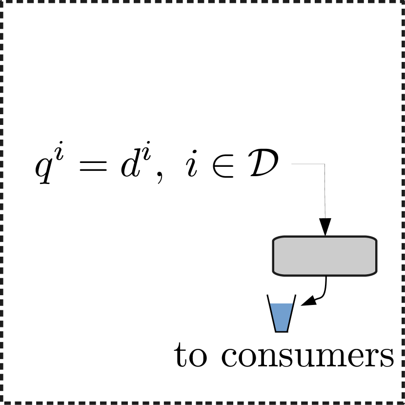
(e) Demand sector

Figure 1: Elements of the water network and the associated flows.

 

Water tanks which play a crucial role in demand management as they ensure water supply, obviate the need for continuous pumping and allow water to be pumped when the price of electricity is lower and provide water in cases of unexpected peaks in demand. Tank dynamics are modelled by simple mass balance equations: let $V^{j}(t)$ be the volume of tank $j=1,\ldots,N_{t}$ at time $t$. We denote all flows in the network by $q^{i}$, $i=1,\ldots,N_{f}$. Let $q^{i}(t)$, $i\in\mathcal{I}_{j}$ be the controlled inflowing streams to tank $j$ and $q^{i}(t)$, $i\in\mathcal{J}_{j}$ be the controlled outflowing streams. Then, the mass balance equation becomes (see Fig. 1(a))

$$\frac{\d{V}^{j}(t)}{\d{t}}=\sum_{i\in\mathcal{I}_{j}}q^{i}(t)-\sum_{i\in\mathcal{J}_{j}}q^{i}(t).$$ (1)

The volume in each tank should never exceed a maximum limit $V^{j}_{\max}$ and it should always be above a hard lower limit $V^{j}_{\min}$, that is,

$$V^{j}_{\min}\leq V^{j}(t)\leq V^{j}_{\max}.$$ (2)

In addition, for the sake of service reliability (availability of water when demand rises unexpectedly) and safety, it is required that the level of water remains above a certain level $V^{j}_{\mathrm{safe}}$. This is allowed to be violated occasionally, when the demand happens to be too high.

Mixing nodes are intersections where flows of water are merged or separated. The mass balance equations for mixing nodes give rise to algebraic constraints of the form

$$\sum_{i\in\mathcal{K}_{s}}q^{i}(t)=\sum_{i\in\mathcal{C}_{s}}q^{i}(t),$$ (3)

where $\mathcal{K}_{s}$ and $\mathcal{C}_{s}$ are the sets of indices of the incoming and outgoing flows at node $s=1,\ldots,N_{s}$ as shown in Fig. 1(b).

Pumps and valves are used to control the flow of water in the network and transfer it across tanks and to the demand sectors. We treat these as controlled systems — indeed, pumping stations and valves are equipped with local controllers — to which we prescribe flow set-points. The local control systems operate at a sampling rate of about $1\,\mathrm{Hz}$, while the operational management of the network updates its decisions at a much slower rate (e.g., hourly). It is reasonable to assume that the local control system equilibrates fast enough to neglect its dynamics in the context of operational control. That said, the flow determined by each pump $i\in\mathcal{P}$ is equal to its prescribed set-point $u^{i}$. As shown in Fig. 1(c), that is

$$q^{i}(t)=u^{i}(t),\ i\in\mathcal{P}.$$ (4)

Similarly, as shown in Fig. 1(d) the flow through each valve is

$$q^{i}(t)=u^{i}(t),\ i\in\mathcal{V}.$$ (5)

All flows in the network are unidirectional, so we require that $q^{i}\geq 0$ for all $i=1,\ldots,N_{f}$. Each pump $i\in\mathcal{P}$ has a maximum pumping capacity $q^{i}_{\max}$, that is we require that

$$0\leq q^{i}(t)\leq q^{i}_{\max},\ i\in\mathcal{P}.$$ (6)

Demand sectors are the exit nodes of the water from the network towards the consumers as shown in Fig. 1(e). At each demand sector $i\in\mathcal{D}$, the mass balance yields

$$q^{i}(t)=d^{i}(t),\ i\in\mathcal{D}.$$ (7)

We treat $d^{i}(t)$ as a random process and elaborate on that in Section 2.2.

We may now describe the system dynamics in terms of the state variable $x(t)=(V^{j}(t))_{j=1,\ldots,N_{t}}$, the input variable $u(t)=(u^{j}(t))_{j\in\mathcal{P}\cup\mathcal{V}}$ and the disturbance $d(t)=(d^{i}(t))_{i\in\mathcal{D}}$. Let $n_{u}=|\mathcal{P}\cup\mathcal{V}|$ be the dimension of $u(t)$, that is, the total number of pumps and valves. Let $n_{d}=|\mathcal{D}|$ be the total number of demand nodes. By discretizing the dynamical equation (1) using the exact discretization method [39, Sec. 4.2.1] and taking into account the algebraic constraints stated above, we may write the system dynamics in the following form of a discrete-time linear time-invariant system

$$x_{k+1} =Ax_{k}+Bu_{k}+G_{d}d_{k},$$ (8a)

$$0 =Eu_{k}+E_{d}d_{k},$$ (8b)

where $A\in\Re^{N_{t}\times N_{t}}$, $B\in\Re^{N_{t}\times n_{u}}$, $G_{d}\in\Re^{N_{t}\times n_{d}}$, $E\in\Re^{N_{s}\times n_{u}}$ and $E_{d}\in\Re^{N_{s}\times n_{d}}$.

The constraints on $x_{k}$ and $u_{k}$ can be concisely written as

$$x_{\min}\leq x_{k}\leq x_{\max},$$ (9a)

$$u_{\min}\leq u_{k}\leq u_{\max},$$ (9b)

with $x_{\min},\,x_{\max}\in\Re^{N_{t}}$ and $u_{\min},\,u_{\max}\in\Re^{n_{u}}$ and $\leq$ is meant in the element-wise sense. These constraints encompass (2) and (6).

2.2 Demands and Electricity Prices

Water demand has been the main source of uncertainty for the operation of drinking water networks and a lot of attention has been paid on the development of models for its prediction. Prediction methodologies span from simple linear models [40] to neural networks [41, 42] and support vector machines [43, 44], nonlinear multiple linear regression [45], Holt-Winters-type models [46], as well as more complex neuro-fuzzy models [47, 48]. Increased predictive ability can be obtained using exogenous information such as weather forecasts [49] and calendar data [5].

In the context of a deregulated wholesale energy market, prices on the day-ahead market are volatile and are often decided on the basis of an auction (bid-based market) among energy companies instead of bilateral agreements with an energy provider. In such cases, energy prices may change on a daily or hourly basis [50]. It is then necessary to be able to predict the day-ahead evolution of the prices using past data; several time series analysis methodologies have been developed for that purpose — see [51] and references therein.

In our approach the prediction procedure is decoupled from the control which allows the use of any forecasting methodology without having to modify the controller parameters or implementation. An independent forecaster provides estimates of future demands and electricity prices along with an estimation of their uncertainty which is discussed in the next section. At time $k$, the predicted demands for the future time $k+j$ are estimated by a model which computes $\hat{d}_{k+j{}\mid{}k}$. Likewise, we denote the predicted electricity prices by $\hat{\alpha}_{k+j{}\mid{}k}$. Let $d_{k+j}$ and $\alpha_{k+j}$ denote the actual, but unknown at time $k$, values of the water demands and prices. Then

$$\begin{bmatrix}d_{k+j}\\ \alpha_{k+j}\end{bmatrix}=\begin{bmatrix}\hat{d}_{k+j{}\mid{}k}\\ \hat{\alpha}_{k+j{}\mid k}\end{bmatrix}+\epsilon_{j{}\mid{}k},$$ (10)

where $\epsilon_{j{}\mid{}k}$ is a random variable which corresponds to the $j$-step-ahead prediction error at time $k$. At time $k$, a forecaster provides finite-horizon estimates of the upcoming water demands and electricity prices

$$\mathchoice{\text{\boldmath{$\displaystyle\hat{d}$}}}{\text{\boldmath{$\textstyle\hat{d}$}}}{\text{\boldmath{$\textstyle\hat{d}$}}}{\text{\boldmath{$\textstyle\hat{d}$}}}_{k}=(\hat{d}_{k+1{}\mid{}k},\hat{\alpha}_{k+1{}\mid k},\ldots,\hat{d}_{k+H_{p}{}\mid{}k},\hat{\alpha}_{k+H_{p}{}\mid k}),$$ (11)

where $H_{p}$ is a prediction horizon. This information will then be provided to the controller as we shall discuss in Section 3.

2.3 Uncertainty

It is common in stochastic control-oriented modeling to assume that the errors $\epsilon_{j{}\mid{}k}$ are independently distributed [18, 19]. This assumption however neglects the covariance across the times stages — indeed, if at the future time $j=1$ the model has a large prediction error we would rather expect that the prediction error at time $j=2$ is likely to be large too. This motivates the use of scenario trees: discrete representations of the random processes $(\epsilon_{j{}\mid{}k})_{j}$ which capture such multistage covariances [52].

To date, stochastic modeling for drinking water networks in presence of price uncertainty has received little attention — to the best of the authors’ knowledge, [53] is the only relevant reference — and the scenario tree approach has not been used previously.

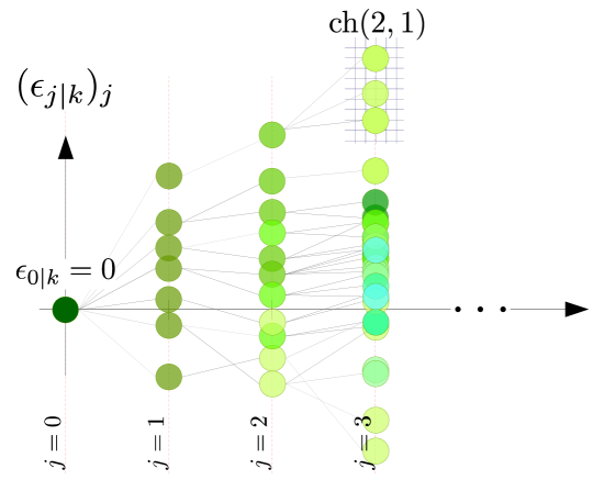
Figure 2: Scenario tree of the random process $(\epsilon_{j{}\mid{}k})_{j}$. At time $j=0$, the prediction error is $\epsilon_{0\mid k}=0$; this defines the root node of the tree. The children nodes $\operatorname{ch}(2,1)$ of node $(2,1)$ are highlighted in the figure.

A scenario tree is a structure such as the one illustrated in Fig. 2. The scenario tree is organised into time instants $j=0,\ldots,H_{p}$ called stages and a number of nodes at each stage denoted by $\epsilon_{j{}\mid{}k}^{i}$ — these are treated as the possible values of $\epsilon_{j{\mid}k}$. At time $j=0$, the prediction error is always equal to $0$ assuming that we observe the current water demands and electricity prices. The corresponding unique node is called the root node of the tree. The nodes of the tree at the last stage are known as leaf nodes. The number of nodes at stage $j$ is denoted by $\mu_{j}$. All nodes are identified by a pair $\alpha=(j,i)$, where $j=0,\ldots,H_{p}$ is the stage index and $i$ is the index of the node in that stage. Each non-leaf node defines a (nonempty) set of children $\operatorname{ch}(j,i)$ which are those nodes in next $j+1$ which are linked to $(j,i)$. Conversely, each not except for the root node defines a unique ancestor denoted by $\operatorname{anc}(j,i)$. The probability of visiting a node $(j,i)$ starting from the root node and following the tree structure is denoted by $p_{j}^{i}$.

Note that the joint demand-price modeling of the uncertainty allows us to cast possible demand-price correlations as in cases of uncertain volume-based pricing.

Using the scenario tree structure, equation (10) yields

$$\begin{bmatrix}d_{k+j}^{i}\\ \alpha_{k+j}^{i}\end{bmatrix}=\begin{bmatrix}\hat{d}_{k+j{}\mid{}k}\\ \hat{\alpha}_{k+j{}\mid k}\end{bmatrix}+\epsilon_{j{}\mid{}k}^{i},$$ (12)

where $j=0,\ldots,H_{p}$ and $i=1,\ldots,\mu_{j}$. Here we see that the tree structure of $\epsilon_{j\mid k}^{i}$ induces a corresponding tree structure upon the water demands and electricity prices, namely $d_{k+j}^{i}$ and $\alpha_{k+j}^{i}$. These are the contingent future water demand and electricity price values associated with the prediction error $\epsilon_{j\mid k}^{i}$.

Similarly, equation (8b) gives

$$Eu_{k+j{}\mid{}k}^{i}+E_{d}d_{k+j{}\mid{}k}^{i}=0,$$ (13)

where $(u_{k+j{}\mid{}k}^{i})_{j,i}$ become the decision variables of the stochastic optimal control problem we shall present in the following section. The discrete-time system dynamics (8a) becomes

$$x_{k+j+1{}\mid{}k}^{l}=Ax_{k+j{}\mid{}k}^{i}+Bu_{k+j{}\mid{}k}^{l}+G_{d}d_{k+j{}\mid{}k}^{l},$$ (14)

where $(j+1,l)\in\operatorname{ch}(j,i)$.

Scenario trees can be constructed from observed sequences of prediction errors which can be easily obtained in practice using methodologies such as [54] or the popular scenario reduction method [55]. There exist several other scenario generation algorithms such as clustering-based algorithms [56, 57] and simulation and optimization-based approaches [58, 59]. It is not necessary, however, to update the scenario tree for $\epsilon_{j{}\mid{}k}$ at every time instant $k$ — it should be updated occasionally to detect changes in the predictive ability of the forecaster or whenever the predictive model is updated.

3 Scenario-based stochastic optimal control

3.1 Control Objectives

The cost for the operation of the water network is quantified in terms of three individual costs which have been proposed in the literature [5, 60, 16, 61]: the economic cost which is related to the treatment cost and electricity required for pumping, the smooth operating cost which penalizes the abrupt operation of pumps and valves and the safety storage cost which penalizes the use of water from the reserves (i.e., allowing the level in the tanks to drop below the safety level).

The economic cost quantifies the production and distribution cost and it is computed by

$$\ell^{w}(u_{k},k)=W_{\alpha}(\alpha_{0}+\alpha_{k})^{\prime}u_{k},$$ (15)

where $\alpha_{0}^{\prime}u_{k}$ is the water production cost (treatment and acquisition fees), $\alpha_{k}^{\prime}u_{k}$ is the uncertain pumping cost and $W_{\alpha}$ is a positive scaling factor.

The smooth operation cost is defined as

$$\ell^{\Delta}(\Delta u_{k})=\Delta u_{k}^{\prime}W_{u}\Delta u_{k},$$ (16)

where $\Delta u_{k}=u_{k}-u_{k-1}$ and $W_{u}\in\Re^{n_{u}\times n_{u}}$ is a symmetric positive definite weight matrix.

The total stage cost at a time instant $k$ is the summation of the above costs and is given by

$$\ell(u_{k},u_{k-1},k)=\ell^{w}(u_{k},k)+\ell^{\Delta}(\Delta u_{k}).$$

The safety storage cost penalizes the drop of water level in the tanks below a given safety level $x_{s}$. An elevation above this safety level ensures that there will be enough water in unforeseen cases of unexpectedly high demand and also maintains a minimum pressure for the flow of water in the network. This is given by

$$\ell^{S}(x_{k})=W_{s}\|\max\{0,x_{s}-x_{k}\}\|,$$ (17)

where $W_{s}$ is a positive scaling factor.

The state constraints (9a) should be satisfied at all times without however jeopardizing the feasibility of the optimal control problem we have to solve at every time instant. For that, we introduce an additional cost which penalizes the violation of the state constraints as follows

$$\ell^{x}(x_{k}) =W_{x}\big{(}\|\max\{0,x_{\min}-x_{k}\}\|$$

$$\qquad\ +\|\max\{0,x_{k}-x_{\max}\}\|\big{)},$$ (18)

where $W_{x}$ is a positive weight factor.

The scaling factors $W_{\alpha}$, $W_{u}$, $W_{s}$ and $W_{x}$ are the tuning knobs of stochastic MPC as we shall discuss in the following section.

3.2 Stochastic optimal control: problem formulation

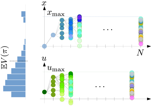
Figure 3: The concept of scenario-based stochastic optimal control: at every time instant $k$, we make an optimal contingency plan by minimizing the expectation of a cost function $V$ which encodes the operation cost along a finite prediction horizon.

In scenario-based stochastic MPC, at every time instant $k$ we solve a stochastic optimal control problem which consists in determining an optimal contingency plan for the future course of actions in a causal fashion, that is, our future decisions $u_{k+j{}\mid{}k}$ are only allowed to depend on information that will be available to the controller at time $k+j$ [62]. This was tacitly stated in equation (14). This concept is illustrated in Fig. 3.

We formulate the following scenario-based stochastic MPC problem with a prediction horizon $H_{p}$ and decision variables $\mathchoice{\text{\boldmath{$\displaystyle x$}}}{\text{\boldmath{$\textstyle x$}}}{\text{\boldmath{$\textstyle x$}}}{\text{\boldmath{$\textstyle x$}}}=\{u_{k+j\mid k},x_{k+j+1\mid k}\}_{j=0,\ldots,H_{p}-1}$ where we minimize the expected total cost along the prediction horizon

$$\operatorname*{minimise}_{\mathchoice{\text{\boldmath{$\displaystyle x$}}}{\text{\boldmath{$\textstyle x$}}}{\text{\boldmath{$\textstyle x$}}}{\text{\boldmath{$\textstyle x$}}}}\ \E\left[V(\mathchoice{\text{\boldmath{$\displaystyle x$}}}{\text{\boldmath{$\textstyle x$}}}{\text{\boldmath{$\textstyle x$}}}{\text{\boldmath{$\textstyle x$}}},p,q,k)\right]+V_{s}(\mathchoice{\text{\boldmath{$\displaystyle x$}}}{\text{\boldmath{$\textstyle x$}}}{\text{\boldmath{$\textstyle x$}}}{\text{\boldmath{$\textstyle x$}}}),$$ (19a)

subject to the following constraints

$$x_{k\mid k}=p,\ u_{k-1\mid k}=q,$$ (19b)

$$x_{k+j+1{}\mid{}k}^{l}=Ax_{k+j{}\mid{}k}^{i}+Bu_{k+j{}\mid{}k}^{l}+G_{d}d_{k+j{}\mid{}k}^{l},$$ (19c)

$$Eu_{k+j\mid k}^{i}+E_{d}d_{k+j\mid k}^{i}(\epsilon_{j})=0,$$ (19d)

$$u_{\min}\leq u_{k+j\mid k}\leq u_{\max}^{i}.$$ (19e)

In (19a), $\E$ is the expectation operator, $V$ is the cost function given by

$$V(\mathchoice{\text{\boldmath{$\displaystyle x$}}}{\text{\boldmath{$\textstyle x$}}}{\text{\boldmath{$\textstyle x$}}}{\text{\boldmath{$\textstyle x$}}},p,q,k)=\sum_{j=0}^{H_{p}-1}\ell(u_{k+j\mid k},u_{k+j-1\mid k},k{+}j),$$ (20)

and $V_{s}$ is the total state constraint violation penalty defined as

$$V_{s}(\mathchoice{\text{\boldmath{$\displaystyle x$}}}{\text{\boldmath{$\textstyle x$}}}{\text{\boldmath{$\textstyle x$}}}{\text{\boldmath{$\textstyle x$}}})=\sum_{j=0}^{H_{p}}\sum_{i=1}^{\mu_{j-1}}\ell^{x}(x_{k+j\mid k}^{i})+\ell^{S}(x_{k+j\mid k}^{i}).$$ (21)

Note that we have a time-varying cost as the electricity prices change with time.

4 Numerical Algorithm

4.1 Problem reformulation

Most modern numerical optimization algorithms such as the (accelerated) proximal gradient algorithm, the alternating directions method of multipliers (ADMM) [63], the Pock-Chambolle method [64], Tseng’s forward-backward-forward algorithm [65] and many another require that the optimization problem be first written in a form

$$\mathcal{P}:\ \operatorname*{minimise}_{\mathchoice{\text{\boldmath{$\displaystyle x$}}}{\text{\boldmath{$\textstyle x$}}}{\text{\boldmath{$\textstyle x$}}}{\text{\boldmath{$\textstyle x$}}}\in\Re^{n}}\,f(\mathchoice{\text{\boldmath{$\displaystyle x$}}}{\text{\boldmath{$\textstyle x$}}}{\text{\boldmath{$\textstyle x$}}}{\text{\boldmath{$\textstyle x$}}})+g(H\mathchoice{\text{\boldmath{$\displaystyle x$}}}{\text{\boldmath{$\textstyle x$}}}{\text{\boldmath{$\textstyle x$}}}{\text{\boldmath{$\textstyle x$}}}),$$ (22)

where $f:\Re^{n}\to\barre\dfn\Re\cup\{+\infty\}$ and $g:\Re^{m}\to\barre$ are convex, lower semi-continuous extended-real-valued functions and $H:\Re^{n}\to\Re^{m}$ is a linear operator. Functions $f$ and $g$ are allowed to return the value $+\infty$ to encode constraints; for example, the constraint $x\in C$ is encoded by the indicator function of the set $C$ which is

$$\delta(x{}\mid{}C)=\begin{cases}0,&\text{ if }x\in C\\ +\infty,&\text{ otherwise}\end{cases}$$ (23)

The key question is how to split the optimization problem in (19) so that the resulting formulation is amenable to a fast numerical solution with massive parallelization. For reasons that will be elucidated in Section 4.3 we choose $f$ to be the smooth part of the cost (which corresponds to the linear function $\ell^{w}$ and the quadratic function $\ell^{\Delta}$) plus the indicator of the input-disturbance coupling given in (8b) plus the indicator of the system dynamics in (8a), that is $f:\Re^{n}\to\barre$ is defined as

$$f(\mathchoice{\text{\boldmath{$\displaystyle x$}}}{\text{\boldmath{$\textstyle x$}}}{\text{\boldmath{$\textstyle x$}}}{\text{\boldmath{$\textstyle x$}}}) =\delta(u_{j}^{i}|\Phi_{1}(d_{j}^{i}))+\delta(x_{j+1}^{i},u_{j}^{i},x_{j}^{\operatorname{anc}(j+1,i)}|\Phi_{2}(d_{j}^{i}))$$

$$+\sum_{j=0}^{H_{p}{-}1}\sum_{i=1}^{\mu_{j}}p_{j}^{i}(\ell^{w}(u_{j}^{i})+\ell^{\Delta}(\Delta u_{j}^{i})),$$ (24)

where $\Delta u_{j}^{i}=u_{j}^{i}-u_{j-1}^{\operatorname{anc}(j,i)}$ and $\Phi_{1}(d)$ is the affine subspace of $\Re^{n_{u}}$

$$\Phi_{1}(d)=\{u:Eu+E_{d}d=0\},$$ (25)

and $\Phi_{2}(d)$ is the affine subspace of $\Re^{2n_{x}+n_{u}}$ defined by the system dynamics

$$\Phi_{2}(d)=\{(z,x,u):z=Ax+Bu+G_{d}d\}.$$ (26)

Function $g$ is naturally chosen to be the indicator of the set of input constraints plus the total constraint violation penalty function $V_{s}$. Note, however, that the same variable $x_{k+j{}\mid{}k}^{i}$ participates in both functions $\ell^{x}$ and $\ell^{S}$. As we shall explain in Section 4.3, this complicates any computations thereon. For that reason we introduce a linear operator $H:\mathchoice{\text{\boldmath{$\displaystyle x$}}}{\text{\boldmath{$\textstyle x$}}}{\text{\boldmath{$\textstyle x$}}}{\text{\boldmath{$\textstyle x$}}}\mapsto\mathchoice{\text{\boldmath{$\displaystyle y$}}}{\text{\boldmath{$\textstyle y$}}}{\text{\boldmath{$\textstyle y$}}}{\text{\boldmath{$\textstyle y$}}}\dfn H(\mathchoice{\text{\boldmath{$\displaystyle x$}}}{\text{\boldmath{$\textstyle x$}}}{\text{\boldmath{$\textstyle x$}}}{\text{\boldmath{$\textstyle x$}}})$ which maps $x_{k+j{}\mid{}k}^{i}$ to $(x_{k+j{}\mid{}k}^{i},x_{k+j{}\mid{}k}^{i})$ and $u_{k+j{}\mid{}k}^{i}$ to itself, that is

$$y_{k+j{}\mid{}k}^{i}=(x_{k+j{}\mid{}k}^{i},x_{k+j{}\mid{}k}^{i},u_{k+j{}\mid{}k}^{i}),$$ (27a)

for $$j=0,\ldots,H_{p}-1$$ and

$$y_{k+H_{p}{}\mid{}k}^{i}=(x_{k+H_{p}{}\mid{}k}^{i},x_{k+H_{p}{}\mid{}k}^{i}).$$ (27b)

Then, we define the function $g:\Re^{m}\to\barre$

$$g(\mathchoice{\text{\boldmath{$\displaystyle y$}}}{\text{\boldmath{$\textstyle y$}}}{\text{\boldmath{$\textstyle y$}}}{\text{\boldmath{$\textstyle y$}}}) =\sum_{\begin{subarray}{c}j=0,\ldots,H_{p}\\ i=1,\ldots,\mu_{j-1}\end{subarray}}\ell^{x}(y_{k+j\mid k}^{i,(1)})+\ell^{S}(y_{k+j\mid k}^{i,(2)})$$

$$+\sum_{\begin{subarray}{c}j=0,\ldots,H_{p}-1\\ i=1,\ldots,\mu_{j-1}\end{subarray}}\delta(y_{k+j\mid k}^{i,(3)}{}\mid{}\mathcal{U}),$$ (28)

where $\mathcal{U}\dfn\{u\in\Re^{n_{u}}{}\mid{}u_{\min}\leq u\leq u_{\max}\}$.

The scenario-based optimization problem (19) is now in the form (22) with $f$ and $g$ given by (24) and (4.1) respectively and $H$ given by (27).

4.2 Convex conjugates and proximal operators

Before we can proceed with the statement of the numerical algorithm for the solution of problem (22) we need to introduce a few mathematical notions. A function $f:\Re^{n}\to\barre$ is called proper if it is not everywhere equal to $+\infty$. It is called lower semi-continuous if for every $x\in\Re^{n}$, $\liminf_{z\to x}f(z)=f(x)$. The domain of $f$ is the set $\operatorname{dom}f\dfn\{x\in\Re^{n}{}\mid{}f(x)<\infty\}$. It is called $\kappa$-strongly convex, for some $\kappa>0$, if the function $f(x)-\nicefrac{{\kappa}}{{2}}\|x\|^{2}$ is convex.

For a proper, convex, lower semi-continuous function $f$, we define its convex conjugate to be the convex function $f^{*}:\Re^{n}\to\barre$ defined as [66, Ch. 11]

$$f^{*}(y)=\sup_{x\in\Re^{n}}\ y^{\prime}x-f(x).$$ (29)

An important property is that if $f$ is $\kappa$-strongly convex, then $f^{*}$ is differentiable with $\nicefrac{{1}}{{\kappa}}$-Lipschitz gradient [66, Prop. 12.60] and the gradient of $f^{*}$ is

$$\nabla f^{*}(y)=\operatorname*{\arg\!\max}_{x\in\Re^{n}}\ y^{\prime}x-f(x).$$ (30)

By means of the convex conjugate we may derive the Fenchel dual optimization problem of (22) which is [67, Sec. 15.3]

$$\mathcal{D}:\ \operatorname*{minimise}_{y\in\Re^{m}}f^{*}(-H^{\prime}y)+g^{*}(y).$$ (31)

Fenchel duality offers a more powerful framework as compared to the classical Lagrangian duality approach as it allows us to dualise functions (by means of their convex conjugates) rather than merely constraints.

Under certain conditions on $f$ and $g$ (see Section 4.3), the two problems are equivalent: their optimal values are equal and given a dual-optimal point $y^{\star}$ which is a minimizer of (31), the optimal solution of $\mathcal{P}$ is $x^{\star}=\nabla f^{*}(-H^{\prime}y^{\star})$. This is referred to as strong duality. The reason why we formulate the dual optimization problem $\mathcal{D}$ is because it possesses a favorable structure which can be exploited in the development of fast and parallelizable numerical algorithms (See Section 4.3).

Lastly, for a proper, lower semi-continuous, extended-real valued function $g:\Re^{m}\to\barre$ we define its proximal operator with parameter $\gamma>0$ to be a function $\operatorname{prox}_{\gamma g}:\Re^{m}\to\Re^{m}$ defined as

$$\operatorname{prox}_{\gamma g}(v)\dfn\operatorname*{\arg\!\min}_{x\in\Re^{m}}g(x)+\nicefrac{{1}}{{2\gamma}}\|x-v\|^{2}.$$ (32)

Proximal mappings act as generalized projections. For example, the proximal mapping of the indicator function $\delta({\,}{\cdot}{\,}{\mid}{\,}C)$ — cf. (23) — of a nonempty, closed, convex set is the projection onto that set, i.e., $\operatorname{prox}_{\gamma\delta({}{\cdot}{}\mid{}D)}(v)=\operatorname{proj}(v{}{\mid}{}C)$.

The proximal operators of many convex functions (such as Euclidean norm, norm-1, quadratic and linear functions, distance-to-set functions) are easy to compute and typically consist in element-wise operations which can be fully parallelized on a GPU. We shall refer to such functions as prox-friendly [68].

So long as $\operatorname{prox}_{\gamma g}$ is easy to compute, so is $\operatorname{prox}_{\gamma g^{*}}$ and it can be obtained from the Moreau decomposition formula which is

$$\operatorname{prox}_{\gamma g}(v)+\gamma\operatorname{prox}_{\gamma^{-1}g^{*}}(\nicefrac{{v}}{{\gamma}})=v.$$ (33)

4.3 Accelerated proximal algorithm on the dual optimization problem

The function $f(\mathchoice{\text{\boldmath{$\displaystyle x$}}}{\text{\boldmath{$\textstyle x$}}}{\text{\boldmath{$\textstyle x$}}}{\text{\boldmath{$\textstyle x$}}})+g(H\mathchoice{\text{\boldmath{$\displaystyle x$}}}{\text{\boldmath{$\textstyle x$}}}{\text{\boldmath{$\textstyle x$}}}{\text{\boldmath{$\textstyle x$}}})$, with $f$ and $g$ defined by (24) and (4.1) respectively, is proper, convex and piecewise linear-quadratic on its domain, so, following [66, Thm. 11.42] there is strong duality. As discussed above, since $f$ is strongly convex, $f^{*}$ is differentiable with Lipschitz gradient. Function $g$ is written in the form of a separable sum — a sum of prox-friendly functions of different arguments [63]. Function $g$ is indeed prox-friendly. Let $(\operatorname{prox}_{\gamma g}(v))_{j,i,(s)}$ denote the part of the vector $\operatorname{prox}_{\gamma g}(v)\in\Re^{m}$, indexed by $j$, $i$ and $s$, which corresponds to $y_{k+j{}\mid{}k}^{i,(s)}$, for $s=1,2,3$. Then, $(\operatorname{prox}_{\gamma g}(v))_{j,i,(1)}$ and $(\operatorname{prox}_{\gamma g}(v))_{j,i,(2)}$ are computed by virtue of the formula

$$\operatorname{prox}_{\gamma\operatorname{dist}(\cdot\mid C)}(v)$$

$$=\begin{cases}v+\frac{\operatorname{proj}_{C}(v)-v}{\operatorname{dist}(v{}\mid{}C)},&\text{if }\operatorname{dist}(v{}{\mid}{}C)>\gamma\\ \operatorname{proj}_{C}(v),&\text{otherwise}\end{cases}$$ (34)

where $\operatorname{dist}(\cdot{}\mid{}C)$ is the distance-to-set function and the fact that $\ell^{x}(x)=W_{x}\operatorname{dist}(x\mid[x_{\min},x_{\max}])$ and $\ell^{S}(x)=W_{s}\operatorname{dist}(x\mid[x_{s},+\infty))$. The proximal operator $(\operatorname{prox}_{\gamma g}(v))_{j,i,(3)}$ is simply the projection on $\mathcal{U}$.

Note that although $g$ is prox-friendly, $g$ composed with the linear operator $H$ — as it is in (22) — is not. This is the main reason why we resort to the dual problem (31).

Given the properties of functions $f^{*}$, being differentiable with Lipschitz gradient, and $g^{*}$, being prox-friendly, we may use Nesterov’s accelerated proximal gradient method on the dual problem which produces the sequence

$$w^{\nu} =y^{\nu}+\beta_{\nu}(y^{\nu}-y^{\nu-1}),$$ (35a)

$$y^{\nu} =\operatorname{prox}_{\gamma g^{*}}(w^{\nu}+\gamma H\nabla f^{*}(-H^{\prime}w^{\nu})),$$ (35b)

with $y^{0}=0$, $y^{-1}=0$, $\beta^{0}=0$. In (35a) we perform an extrapolation step for some $\beta_{\nu}>0$ and we perform a dual gradient projection update on the extrapolated vector $w^{\nu}$. The extrapolation parameters $\beta-\nu$ are parametrized as $\beta^{\nu}=\theta_{\nu}(\theta_{\nu-1}^{-1}-1)$ with $\theta_{0}=\theta_{-1}=1$. Any choice of $\theta_{\nu}$ so that $1-\theta_{\nu+1}\leq\nicefrac{{\theta_{\nu+1}^{2}}}{{\theta_{\nu}^{2}}}$. A simple choice is

$$\theta_{\nu}=\frac{2}{\nu+2},$$ (36)

for $\nu\geq 1$. Here we choose $\theta_{\nu+1}=\nicefrac{{1}}{{2}}(\sqrt{\theta_{\nu}^{4}+4\theta_{\nu}^{2}}-\theta_{\nu}^{2})$ which satisfies the above requirement with equality.

This algorithm fits into Tseng’s Alternating Minimization framework [69, 70]. It has been found to be suitable for embedded applications as it is relatively simple to implement and it has good convergence properties (the dual variable $y^{\nu}$ converges with rate $O(\nicefrac{{1}}{{\nu^{2}}})$ and an averaged primal iterate converges at $O(\nicefrac{{1}}{{\nu^{2}}})$ as well) [71]. It involves only matrix-vector operations (additions and multiplications) and it is numerically stable. In the following section we discuss how the involved operations can be massively parallelized in a lock-step fashion (performing the exact same operation on different memory positions) and how the algorithm can be implemented on a GPU.

4.4 Implementation

Because of the definition of $f$ in (24), the computation of the gradient of $f^{*}$ as defined in problem (30) boils down to the solution of a scenario-based optimal control problem where the only constraints are the ones defined by the system dynamics. This problem can be solved by dynamic programming leading to a Riccati-type recursion from stage $k=H_{p}$ to stage $k=0$. At each stage operations across all nodes can be fully parallelized. In particular, such a parallelization — assuming that full parallelization is supported by the hardware — equalizes the complexity of the scenario-based Riccati recursion to that of a deterministic one. A detailed exposition of the details of this procedure is available in [22, 9].

All operations involved in the computation of $\operatorname{prox}_{\gamma g}$ are element-wise operations and can be fully parallelized on a GPU; therefore, the computational cost for applying $\operatorname{prox}_{\gamma g}$ — or, what is the same — $\operatorname{prox}_{\gamma^{-1}g^{*}}$ via (33) is negligible.

5 Functionality

In this section we present RapidNet, a CUDA-C++ implementation of the accelerated proximal gradient method for the solution of scenario-based stochastic optimal control problems, particularly tailored to the needs of a drinking water network.

5.1 Software structure

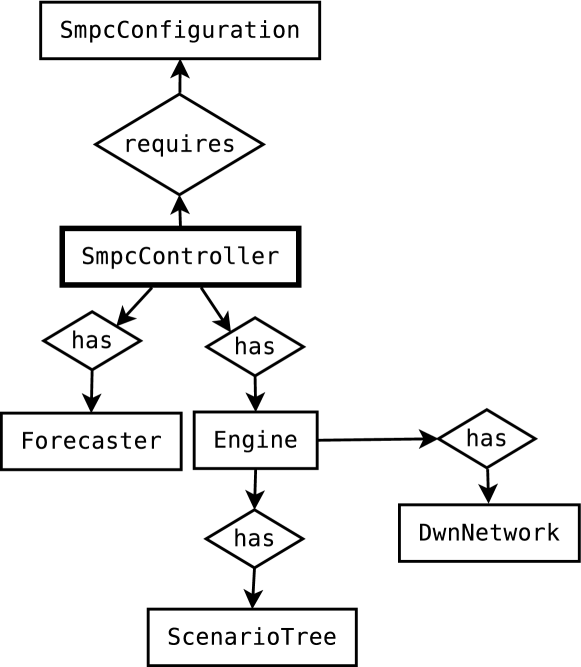
Figure 4: Entity-Relationship (ER) diagram of the entities in RapidNet which reflects the underlying class structure.

The entities involved in RapidNet and the relationships among each other are illustrated in Fig. 4 which correspond to classes in the CUDA-C++ implementation of RapidNet (see also Table 1).

Table 1: Description of the major class and the associated JSON files in RapidNet.

Class name	Description	JSON file
SmpcController	Runs the accelerated dual proximal gradient algorithm can computes a control action to be applied to the water network. Computations are carried out on GPU and the output (flow set-points) can be stored in a JSON file.	controlOutput.json
DwnNetwork	Encapsulates all information related to the topology, dynamics and constraints of the water network.	network.json
ScenarioTree	Scenario-tree representation of the uncertainty in electricity prices and water demands.	scenarioTree.json
Forecaster	An abstract forecaster which predicts the upcoming electricity prices and water demands using some predictive model (implemented by subclassing Forecaster) or reads the forecasts from a JSON file (so that the user can use forecasts from third-party software).	forecaster.json
Engine	Provides essential functionality to SmpcController and manages the GPU-side memory.
SmpcConfiguration	Contains configuration parameters that are relevant for SmpcController (tuning parameters, solver tolerance, maximum number of iterations).	controllerconfig.json

 

The DwnNetwork class stores data related to the network topology, physical constraints and network dynamics matrices in equations (8a) and (8b). The user can create instances of DwnNetwork simply by passing a JSON file, network.json, with the network information.

The ScenarioTree class models the scenario tree structure that represents the uncertainty associated with the volatile energy prices and water demands. This class describes the structure of the scenario tree by assigning a unique index to each node and storing the indexes of the children of each non-leaf node, the ancestor of all nodes except for the root node and the values $d_{k+j\mid k}^{i}$ and $\alpha_{k+j\mid k}^{i}$ at each node $(j,i)$. An instance of ScenarioTree can be generated using a JSON file, scenarioTree.json.

An SmpcController executes the accelerated proximal gradient algorithm to solve a stochastic optimal control problem at every time instant and compute the control actions to be applied to the water network. Certain functionality is delegated to Engine — a collection of utility methods — which precomputes certain quantities which are associated with the Riccati-type recursion (details can be found in [9]) for the computation of the dual gradient and manages the associated memory on GPU.

The Engine is, in turn, linked with to a DwnNetwork entity which provides all necessary technical specifications for the network (topology, dynamics, constraints) and a ScenarioTree entity which encodes the probabilistic information associated with the prediction errors. Note that the end-user does not have to create instances of Engine or directly interact with it.

A Forecaster provides to the controller estimates of the upcoming water demands and electricity prices. This is an abstract class which can be subclassed with particular model implementations (e.g., ARIMA, SVM, or any other), or the user can provide custom forecasts using any third-party software which exports its forecasts in a JSON file.

SmpcController requires certain configuration parameters which is provided by the entity SmpcConfiguration. There, the user specifies the desired tolerance, maximum number of iterations and can override other solver-specific properties.

Overall, the flow of information in RapidNet is shown in Fig. 5. The end-user initializes an SmpcController object by providing the network topology, the controller configuration and a scenario tree. During real-time operation, the controller receives the network state $x_{k}$ (which can be provided in a JSON file) and, using a demand/price forecaster, computes a control action which is applied to the system.

In Table 2 we list the main methods of RapidNet. Additional getter methods are available in each class for more advanced use-case scenarios.

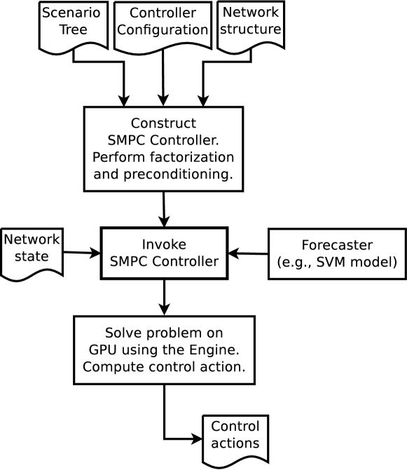
Figure 5: Flow of information in RapidNet.

Table 2: Key methods in RapidNet.

Class	Method	Description
SmpcController	controlAction	Computes control action using the accelerated proximal gradient algorithm to solve the scenario-based stochastic optimal control problem.
Forecaster	predictDemand	Returns water demand forecasts.
	predictPrice	Returns energy price forecasts.
Engine	factorStep	Precomputes certain quantities that facilitate and accelerate the computation of the dual gradient in the algorithm.

 

5.2 GPU Implementation

GPUs were first developed for video applications and, due to the high demand in high-performance graphics, rapidly evolved to powerful hardware featuring hundreds of computation cores. Nowadays, GPUs are used for more than video processing and they are becoming popular for computational purposes including, but not limited to, environmental modeling [72, 73, 74]. By design they are well-suited for data-parallel lockstep applications where the same type of operation is applied to different memory positions. Instructions are sent to the GPU (from the CPU) in the form of compute kernels. GPUs offer unprecedented parallelization capabilities provided that the program can be parallelized in a lockstep fashion (the same operation is executed on different memory positions).

CUDA is a parallel computing framework and application programming interface for NVIDIA GPUs used for general-purpose computing. Part of the CUDA framework is cuBLAS, a parallel counterpart of the popular linear algebra library BLAS.

In RapidNet, at every time instant $k$, the method controlAction in SmpcController returns the control action that is to be applied to the water network (pump and valve set points). All computations involved in this method are either summations or matrix-vector multiplications which can be parallelized across the nodes of a stage. These multiplications are implemented using the function cublasSgemmBatched of cuBLAS and vector additions are performed using the cublasSaxpy of cuBLAS. Apart from the standard cuBLAS methods, we have defined custom kernels for the summation over the set of nodes and to evaluate projections with respect to the box constraints and the proximal operator of the distance function from the set (that is, to compute the proximal operator of $g$ as discussed in Section 4.3.

5.3 Software verification

The validation of the software is done through unit testing. A unit represents the smallest functional part of the software and unit testing involves verification of its functionality through predefined inputs and expected outputs. It assists in the debugging and maintenance of the code and facilitates the integration of the various units reliably. In lack of a standardized testing framework for CUDA applications, we developed our in-house testing framework. Moreover, using cudaMemCheck we have thoroughly tested for GPU-side memory leaks.

6 RapidNet in action: Simulation results

Figure 6: Schematic diagram of the drinking water network of Barcelona. Overall, this distribution network involves $63$ tanks, $114$ controlled flows and, in particular, $75$ pumps and $39$ valves, $88$ demand sectors and $17$ mixing nodes.

 

In this section, we present the application of RapidNet for the management of the drinking water network of the city of Barcelona, whose schematic diagram is shown in Fig. 6, using the demand data provided in [75, 9]. The network counts a total of $63$ tanks, $114$ controlled flows (by means of $75$ pumps and $39$ valves), $88$ demand sectors and $17$ mixing nodes.

6.1 Forecasting of water demands

Upcoming water demands are predicted using a radial-basis-function support vector machines (SVM) model from the literature with good predictive ability [5]. The model predicts the water demand using past demand data together with calendar data (day of the week). Validation information is provided in [5]. In Fig. 7 we show an instance of a prediction using this SVM model.

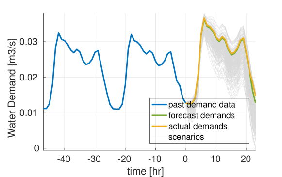
Figure 7: Water demands predicted with a radial-basis-function SVM model. The current time instant is positioned at $0$.

6.2 Forecasting of energy prices

Among other European countries such as Denmark and Sweden, Austria implements a deregulated energy market which induces a volatile stream of electricity prices. Time series of energy prices in Austria have become public by EXAA (Energy Exchange Austria; a central European energy exchange) and are available online at http://www.exaa.at/de/marktdaten/historische-daten (Accessed on ). In lack of electricity price data from Spain or relevant data from the water network of Barcelona, we used price data from Austria as an indicative dataset.

Out of $8784$ hourly price data which are available for the year 2016, we excluded the last $2000$ data points to be used for testing and using the rest of the data we built an ARIMA$(24,1,4)$ model. ARIMA models have been previously used for the short-term prediction of electricity prices in the day-ahead market [51]. Using a Monte-Carlo method, a set of $10^{4}$ independent scenarios were generated and, subsequently, these were reduced into a scenario tree using the method described in [55]. An instance of a prediction using the trained ARIMA model along with the associated scenario tree is shown in Fig. 8.

The residuals of the model where found to be uncorrelated at the confidence level of $99.9\%$. Indeed, the residuals pass the Ljung-Box Q-test of uncorrelatedness with p-value equal to $1.0000$. The model was selected using the Akaike information criterion (AIC) with value $1.523$.

It is natural to expect that the upcoming energy prices can be only predicted up to moderate accuracy as they do not follow a regular pattern and are influenced by many market-related parameters. Despite our limited predictive capacity, we shall show in Section 6.3 that by taking into account this volatility using stochastic model predictive control we do mitigate the effect of the price uncertainty leading to a more economic operation of the water network.

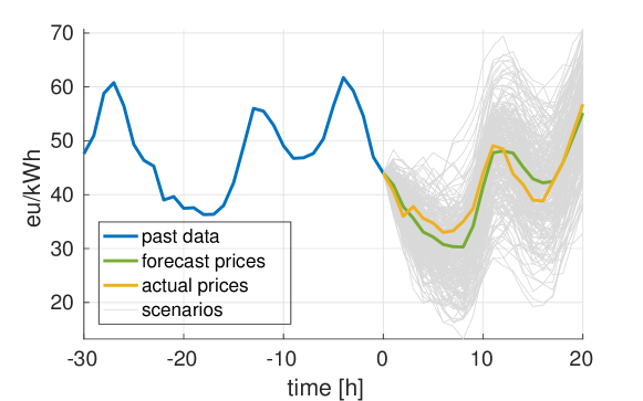
Figure 8: Past data of energy prices (blue line) together with the nominal 24-hour-ahead forecast produced by the ARIMA model (green line) and the actual upcoming price data (orange line). A set of $250$ scenarios in also shown with thin gray lines. The current time instant is positioned at $0$.

6.3 Closed-loop simulations

In this section we present closed-loop simulation results on the water network where the sampling time is equal to $1\,\mathrm{hr}$ and the prediction horizon of the SSMPC was fixed to $H_{p}=24$. The weight parameters used to tune the SSMPC are $W_{\alpha}=10^{6}$, $W_{u}=1.3\cdot 10^{7}\cdot I$, $W_{s}=10^{5}$ and $W_{x}=10^{8}$. Note that all units used in this section are SI units (flows in $\nicefrac{\mathrm{m^{3}}}{\mathrm{s}}$ and volumes in $\mathrm{m^{3}}$).

The system was simulated for a period of $H_{s}=168$ time instants, which corresponds to one week of operation. In order to assess the performance of the closed-loop operation, we use three KPIs, in particular: (i) the economic index which is defined as

$$\mathrm{KPI}_{E}=\nicefrac{{1}}{{H_{s}}}\sum_{k=1}^{H_{s}}(\alpha_{0}+\alpha_{k})^{\prime}u_{k},$$ (37)

which provides an estimation of the average hourly cost of operation of the water network, (ii) the safety index, which is defined as

$$\mathrm{KPI}_{S}=\sum_{k=1}^{H_{s}}\|\max\{x_{s}-x_{k},0\}\|_{1},$$ (38)

which quantifies the total weekly violation of the safety constraint (the “soft” requirement that $x_{k}\geq x_{s}$), and, last, (iii) the complexity index which is the worst-case time required to solve the SSMPC optimization problem up to the specified accuracy, which is defined as

$$\mathrm{KPI}_{\tau}=\max_{k=1,\ldots,H_{s}}\tau_{k},$$ (39)

where $\tau_{k}$ is the computation time required by the solver for solving the SSMPC problem at time instant $k$. The maximum runtime is of higher importance that the average runtime in applications to verify that a decision can be made within the available time period. All three indices are defined so that low values are preferred.

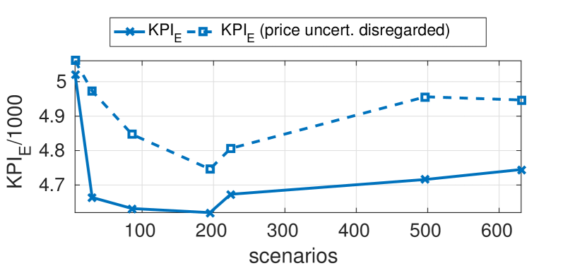
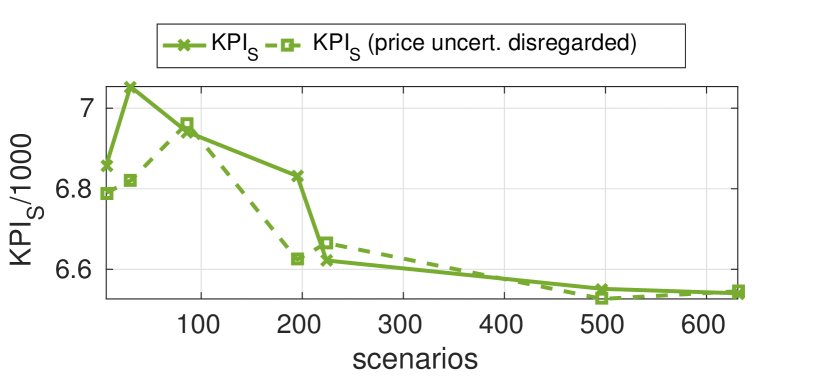
Figure 9: (Up) The economic index $\mathrm{KPI}_{E}$ in euros (€) as a function of the number of scenarios considered in the SSMPC formulation, (Down) The safety index $\mathrm{KPI}_{S}$. The dashed lines correspond to SSMPC’s which do not consider the volatility in electricity prices.

In order to justify the need for and underline the importance of taking into account the uncertainty associated with electricity prices, we performed two sets of simulations where in one case we disregarded that volatility (the SSMPC used only the nominal predictions of the electricity prices). We may observe in Fig. 9 that the hourly operation of the network becomes more expensive by approximately $+5\%$, therefore, the proposed stochastic control approach can lead to significant economic savings for the network operator. For example, for the case of $631$ scenarios, the operation cost when the price uncertainty is disregarded is € 4947/hour, whereas with the proposed approach which takes into account the price uncertainty it drops to € 4748/hour — a saving of € 199/hour, that is, a cost reduction of $4\%$.

We may also see that as more scenarios are considered in the SSMPC formulation, the average cost of operation plummets at around $194$ scenarios, where, however, the safety index is still high. In order to obtain a safer operation we need to pay the “cost of safe operation”: Indeed, at $631$ scenarios, the operation of the network is more expensive compared to the case of $194$ scenarios, but $\mathrm{KPI}_{S}$ is at a minimum. This reflects a trade-off between the economic and safe operation of the network.

At $631$ scenarios, the SSMPC optimization problem involves as many as $2,306,133$ primal variables and $3,126,960$ dual variables. RapidNet solves it with $\mathrm{KPI}_{\tau}=82.7\,\mathrm{s}$ as compared to $\mathrm{KPI}_{\tau}=719\,\mathrm{s}$ for the popular commercial solver Gurobi v7.0 at the same level of accuracy (tolerance $5\cdot 10^{-2}$). The solvers cplex and mosek were also tested, but Gurobi outperformed them consistently. As we may see in Fig. 10, RapidNet exhibits a lower complexity index by approximately an order of magnitude.

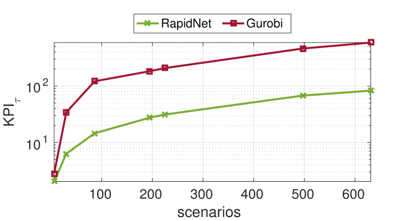
Figure 10: $\mathrm{KPI}_{\tau}$ for Gurobi (executed on an Intel Core i7-6600U machine with 4 $\times$ 2.60GHz CPUs, 12GB RAM running 64-bit Ubuntu 16.04) and RapidNet running on an NVIDIA Tesla C2075 GPU.

7 Conclusions and Future Work

We presented the integrated software solution RapidNet for the control of drinking water networks which accounts for uncertainty both in predicted water demand and in predicted electricity prices in the day-ahead energy market.

RapidNet is a highly inter-operable software as it can be interfaced using JSON files which follow a standard API which is detailed in the software documentation. It can be combined with any forecaster as the controller does not need to know the mechanism with which the forecasts are produced. RapidNet features a parser implemented in MATLAB which allows the conversion of EPANET .inp files to JSON files. It is an open-source and free software which is distributed under the terms of the GNU LGPL v3.0 licence and can be downloaded at https://github.com/GPUEngineering/RapidNet.

In this paper we have shown via simulations that when a water network is operated in the context of a volatile energy market, considerable savings can be obtained by using a predictor of the upcoming energy prices and taking into account the associated price-related uncertainty in the formulation of the scenario tree. Alongside, we advocate that RapidNet can transform SSMPC from a powerful (but too complex) theoretical development to control engineering practice and enabling the solution of very large SSMPC scale problems and their seamless integration into the control system of the water network.

This work focuses on flow-based water distribution networks such as the network of the city of Barcelona. Pressure-based networks lead to optimization problems with nonconvex constraints. These can be approximated by solving a constraints satisfaction problem (CSP) as discussed in [60]. The problem can be then transformed into a convex SSMPC problem which can be solved by RapidNet. The operator splitting concept has been proven to apply to sums of nonconvex functions which allows the solution of nonconvex optimal control problems with input constraints [76]. This allows the application of recent developments in nonconvex optimization such as PANOC [77] for the solution of nonlinear MPC problems.

Future developments in RapidNet will involve the implementation of new faster parallelizable algorithms which make use of quasi-Newton directions based on our recent theoretical work [78] and the exploitation of multiple-GPU architectures. We shall introduce a library of available water network entities from the literature as well as reported water demand and energy price models for different water networks and energy markets.

References

References

- [1] S. Eggimann, L. Mutzner, O. Wani, M. Y. Schneider, D. Spuhler, M. Moy de Vitry, P. Beutler, M. Maurer, The potential of knowing more: A review of data-driven urban water management, Environmental Science & Technology 51 (5) (2017) 2538–2553, pMID: 28125222. doi:10.1021/acs.est.6b04267.
- [2] J. Meseguer, J. Quevedo, Real-time monitoring and control in water systems, in: V. Puig, C. Ocampo-Martínez, R. Pérez, G. Cembrano, J. Quevedo, T. Escobet (Eds.), Real-time Monitoring and Operational Control of Drinking-Water Systems, Springer, Cham, 2017, pp. 1–19. doi:10.1007/978-3-319-50751-4_1.
- [3] D. P. Solomatine, Applications of data-driven modelling and machine learning in control of water resources, in: Computational Intelligence in Control, IGI Global, 2003, pp. 197–217.
- [4] A. H. Lobbrecht, D. P. Solomatine, Machine learning in real-time control of water systems, Urban Water 4 (3) (2002) 283 – 289. doi:10.1016/S1462-0758(02)00023-7.
- [5] A. K. Sampathirao, J. M. Grosso, P. Sopasakis, C. Ocampo-Martinez, A. Bemporad, V. Puig, Water demand forecasting for the optimal operation of large-scale drinking water networks: the Barcelona case study, in: 19th IFAC World Congress, Cape Town, South Africa, 2014, pp. 10457–10462. doi:10.3182/20140824-6-ZA-1003.01343.
- [6] Y. Wang, C. Ocampo-Martinez, V. Puig, Robust model predictive control based on Gaussian processes: Application to drinking water networks, in: 2015 European Control Conference (ECC), 2015, pp. 3292–3297. doi:10.1109/ECC.2015.7331042.
- [7] A. Mesbah, Stochastic model predictive control: An overview and perspectives for future research, IEEE Control Systems 36 (6) (2016) 30–44. doi:10.1109/MCS.2016.2602087.
- [8] H. Mala-Jetmarova, N. Sultanova, D. Savic, Lost in optimisation of water distribution systems? a literature review of system operation, Environmental Modelling & Software 93 (2017) 209 – 254. doi:10.1016/j.envsoft.2017.02.009.
- [9] A. K. Sampathirao, P. Sopasakis, A. Bemporad, P. Patrinos, GPU-accelerated stochastic predictive control of drinking water networks, IEEE Transactions on Control Systems Technology PP (99) (2017) 1–12. doi:10.1109/TCST.2017.2677741.
- [10] G. Calafiore, M. Campi, The scenario approach to robust control design, Automatic Control, IEEE Transactions on 51 (5) (2006) 742–753. doi:10.1109/TAC.2006.875041.
- [11] A. Horne, J. M. Szemis, S. Kaur, J. A. Webb, M. J. Stewardson, A. Costa, N. Boland, Optimization tools for environmental water decisions: A review of strengths, weaknesses, and opportunities to improve adoption, Environmental Modelling & Software 84 (2016) 326 – 338. doi:10.1016/j.envsoft.2016.06.028.
- [12] A. Goryashko, A. Nemirovski, Robust energy cost optimization of water distribution system with uncertain demand, Automation and Remote Control 75 (10) (2014) 1754–1769. doi:10.1134/S000511791410004X.
- [13] J. M. Grosso, J. M. Maestre, C. Ocampo-Martinez, V. Puig, On the assessment of tree-based and chance-constrained predictive control approaches applied to drinking water networks, IFAC Proceedings Volumes 47 (3) (2014) 6240 – 6245. doi:10.3182/20140824-6-ZA-1003.01648.
- [14] C. Ocampo-Martinez, V. Fambrini, D. Barcelli, V. Puig, Model predictive control of drinking water networks: A hierarchical and decentralized approach, in: Proceedings of the 2010 American Control Conference, 2010, pp. 3951–3956. doi:10.1109/ACC.2010.5530643.
- [15] M. Bakker, J. H. G. Vreeburg, L. J. Palmen, V. Sperber, G. Bakker, L. C. Rietveld, Better water quality and higher energy efficiency by using model predictive flow control at water supply systems, Journal of Water Supply: Research and Technology - Aqua 62 (1) (2013) 1–13. doi:10.2166/aqua.2013.063.
- [16] C. Ocampo-Martinez, V. Puig, G. Cembrano, R. Creus, M. Minoves, Improving water management efficiency by using optimization-based control strategies: the Barcelona case study, Water Science and Technology: Water Supply 9 (5) (2009) 565–575. doi:10.2166/ws.2009.524.
- [17] V. Tran, M. Brdys, Optimizing control by robustly feasible model predictive control and application to drinking water distribution systems, in: C. Alippi, M. Polycarpou, C. Panayiotou, G. Ellinas (Eds.), Artificial Neural Networks – ICANN 2009, Vol. 5769 of Lecture Notes in Computer Science, Springer Berlin Heidelberg, 2009, pp. 823–834. doi:10.1007/978-3-642-04277-5_83.
- [18] Y. Wang, C. Ocampo-Martinez, V. Puig, Stochastic model predictive control based on Gaussian processes applied to drinking water networks, IET Control Theory Applications 10 (8) (2016) 947–955. doi:10.1049/iet-cta.2015.0657.
- [19] J. M. Grosso, P. Velarde, C. Ocampo-Martinez, J. M. Maestre, V. Puig, Stochastic model predictive control approaches applied to drinking water networks, Optimal Control Applications and Methods (2016) 1–18doi:10.1002/oca.2269.
- [20] C. J. Hutton, Z. Kapelan, A probabilistic methodology for quantifying, diagnosing and reducing model structural and predictive errors in short term water demand forecasting, Environmental Modelling & Software 66 (2015) 87 – 97. doi:10.1016/j.envsoft.2014.12.021.
- [21] A. Sampathirao, P. Sopasakis, A. Bemporad, P. Patrinos, Fast parallelizable scenario-based stochastic optimization, in: 4th European Conference on Computational Optimization, Leuven, Belgium, 2016.
- [22] A. Sampathirao, P. Sopasakis, A. Bemporad, P. Patrinos, Distributed solution of stochastic optimal control problems on GPUs, in: 54 IEEE Conf. Decision and Control, Osaka, Japan, 2015, pp. 7183–7188. doi:10.1109/CDC.2015.7403352.
- [23] A. Themelis, S. Villa, P. Patrinos, A. Bemporad, Stochastic gradient methods for stochastic model predictive control, in: 2016 European Control Conference (ECC), 2016, pp. 154–159. doi:10.1109/ECC.2016.7810279.
- [24] J. Kang, A. U. Raghunathan, S. Di Cairano, Decomposition via ADMM for scenario-based model predictive control, in: 2015 American Control Conference (ACC), 2015, pp. 1246–1251. doi:10.1109/ACC.2015.7170904.
- [25] P. Carpentier, K. Barty, P. Girardeau, Decomposition of large-scale stochastic optimal control problems, RAIRO - Operations Research 44 (2010) 167–183. doi:10.1051/ro/2010013.
-
[26]
B. Defourny, D. Ernst, L. Wehenkel,
Multistage stochastic programming: A
scenario tree based approach to planning under uncertainty, in: Decision
Theory Models for Applications in Artificial Intelligence, IGI Global,
2012, pp. 97–143.
URL http://hdl.handle.net/2268/80246 - [27] D. R. Jiang, T. V. Pham, W. B. Powell, D. F. Salas, W. R. Scott, A comparison of approximate dynamic programming techniques on benchmark energy storage problems: Does anything work?, in: 2014 IEEE Symposium on Adaptive Dynamic Programming and Reinforcement Learning (ADPRL), 2014, pp. 1–8. doi:10.1109/ADPRL.2014.7010626.
-
[28]
P.-L. Carpentier, M. Gendreau, F. Bastin,
Optimal
scenario set partitioning for multistage stochastic programming with the
progressive hedging algorithm, Tech. rep. (2013).
URL http://www.optimization-online.org/DB_HTML/2013/10/4065.html - [29] D. P. Bertsekas, Dynamic Programming and Optimal Control, 2nd Edition, Athena Scientific, 2000.
- [30] E. Klintberg, S. Gros, A parallelizable interior point method for two-stage robust MPC, IEEE Transactions on Control Systems Technology PP (99) (2017) 1–11. doi:10.1109/TCST.2016.2638680.
- [31] M. Lubin, C. G. Petra, M. Anitescu, V. Zavala, Scalable stochastic optimization of complex energy systems, in: Proceedings of 2011 International Conference for High Performance Computing, Networking, Storage and Analysis, SC ’11, ACM, New York, NY, USA, 2011, pp. 64:1–64:64. doi:10.1145/2063384.2063470.
- [32] J. Kang, Y. Cao, D. P. Word, C. Laird, An interior-point method for efficient solution of block-structured NLP problems using an implicit Schur-complement decomposition, Computers & Chemical Engineering 71 (2014) 563 – 573. doi:10.1016/j.compchemeng.2014.09.013.
- [33] N. Chiang, C. G. Petra, V. M. Zavala, Structured nonconvex optimization of large-scale energy systems using PIPS-NLP, in: Power Systems Computation Conference (PSCC), 2014, 2014, pp. 1–7. doi:10.1109/PSCC.2014.7038374.
-
[34]
J. Hübner, M. Schmidt, M. C. Steinbach,
A
distributed interior-point KKT solver for multistage stochastic
optimization, Optimization Online.
URL http://www.optimization-online.org/DB_HTML/2016/02/5318.html - [35] G. Cembrano, J. Quevedo, V. Puig, R. Pérez, J. Figueras, J. M. Verdejo, I. Escaler, G. Ramón, G. Barnet, P. Rodríguez, M. Casas, PLIO: a generic tool for real-time operational predictive optimal control of water networks, Water Science and Technology 64 (2) (2011) 448–459. doi:10.2166/wst.2011.431.
- [36] C. Hans, P. Sopasakis, A. Bemporad, J. Raisch, C. Reincke-Collon, Scenario-based model predictive operation control of islanded microgrids, in: 54 IEEE Conf. Decision and Control, Osaka, Japan, 2015. doi:10.1109/CDC.2015.7402711.
- [37] E. Batchabani, M. Fuamba, Optimal tank design in water distribution networks: Review of literature and perspectives, Journal of Water Resources Planning and Management 140 (2) (2014) 136–145. doi:10.1061/(asce)wr.1943-5452.0000256.
- [38] M. Papageorgiou, Optimal control of generalized flow networks, in: P. Thoft-Christensen (Ed.), System Modelling and Optimization: Proceedings of the 11th IFIP Conference Copenhagen, Denmark, July 25–29, 1983, Springer Berlin Heidelberg, Berlin, Heidelberg, 1984, pp. 373–382. doi:10.1007/BFb0008911.
- [39] C. Chi-Tsong, Linear System Theory and Design, 3rd Edition, Saunders College Publishing, Philadelphia, PA, USA, 1999.
- [40] D. J. Pedregal, J. R. Trapero, Electricity prices forecasting by automatic dynamic harmonic regression models, Energy Conversion and Management 48 (5) (2007) 1710 – 1719. doi:10.1016/j.enconman.2006.11.004.
- [41] M. Ghiassi, D. K. Zimbra, H. Saidane, Urban water demand forecasting with a dynamic artificial neural network model, Journal of Water Resources Planning and Management 134 (2) (2008) 138–146. doi:10.1061/(asce)0733-9496(2008)134:2(138).
- [42] M. Romano, Z. Kapelan, Adaptive water demand forecasting for near real-time management of smart water distribution systems, Environmental Modelling & Software 60 (2014) 265 – 276. doi:10.1016/j.envsoft.2014.06.016.
- [43] C. Peña-Guzmán, J. Melgarejo, D. Prats, Forecasting water demand in residential, commercial, and industrial zones in Bogotá, Colombia, using least-squares support vector machines, Mathematical Problems in Engineering 2016 (2016) 1–10. doi:10.1155/2016/5712347.
- [44] I. S. Msiza, F. V. Nelwamondo, T. Marwala, Artificial neural networks and support vector machines for water demand time series forecasting, in: 2007 IEEE International Conference on Systems, Man and Cybernetics, 2007, pp. 638–643. doi:10.1109/ICSMC.2007.4413591.
- [45] A. Yasar, M. Bilgili, E. Simsek, Water demand forecasting based on stepwise multiple nonlinear regression analysis, Arabian Journal for Science and Engineering 37 (8) (2012) 2333–2341. doi:10.1007/s13369-012-0309-z.
- [46] Y. Wang, C. Ocampo-Martínez, V. Puig, J. Quevedo, Gaussian-process-based demand forecasting for predictive control of drinking water networks, in: C. G. Panayiotou, G. Ellinas, E. Kyriakides, M. M. Polycarpou (Eds.), Critical Information Infrastructures Security: 9th International Conference, CRITIS 2014, Limassol, Cyprus, October 13-15, 2014, Revised Selected Papers, Springer International Publishing, Cham, 2016, pp. 69–80. doi:10.1007/978-3-319-31664-2_8.
- [47] E. I. Papageorgiou, K. Poczȩta, C. Laspidou, Hybrid model for water demand prediction based on fuzzy cognitive maps and artificial neural networks, in: 2016 IEEE International Conference on Fuzzy Systems (FUZZ-IEEE), 2016, pp. 1523–1530. doi:10.1109/FUZZ-IEEE.2016.7737871.
- [48] N. Lertpalangsunti, C. W. Chan, R. Mason, P. Tontiwachwuthikul, A toolset for construction of hybrid intelligent forecasting systems: application for water demand prediction, Artificial Intelligence in Engineering 13 (1) (1999) 21 – 42. doi:10.1016/S0954-1810(98)00008-9.
- [49] M. Bakker, H. van Duist, K. van Schagen, J. Vreeburg, L. Rietveld, Improving the performance of water demand forecasting models by using weather input, Procedia Engineering 70 (2014) 93 – 102. doi:10.1016/j.proeng.2014.02.012.
- [50] L. Puglia, P. Patrinos, D. Bernardini, A. Bemporad, Reliability and efficiency for market parties in power systems, in: 2013 10th International Conference on the European Energy Market (EEM), 2013, pp. 1–8. doi:10.1109/EEM.2013.6607416.
- [51] R. Weron, Electricity price forecasting: A review of the state-of-the-art with a look into the future, International Journal of Forecasting 30 (4) (2014) 1030 – 1081. doi:10.1016/j.ijforecast.2014.08.008.
- [52] A. Shapiro, D. Dentcheva, A. Ruszczynski, Lectures on Stochastic Programming: Modeling and Theory, Society for Industrial and Applied Mathematics, Philadelphia, 2009. doi:10.1137/1.9780898718751.
- [53] B. Eck, S. McKenna, A. Akrhiev, A. Kishimoto, P. Palmes, N. Taheri, S. van den Heever, Pump scheduling for uncertain electricity prices, in: World Environmental and Water Resources Congress 2014, American Society of Civil Engineers, 2014. doi:10.1061/9780784413548.046.
- [54] G. C. Pflug, A. Pichler, Dynamic generation of scenario trees, Computational Optimization and Applications 62 (3) (2015) 641–668. doi:10.1007/s10589-015-9758-0.
- [55] H. Heitsch, W. Römisch, Scenario tree modeling for multistage stochastic programs, Mathematical Programming 118 (2) (2009) 371–406. doi:10.1007/s10107-007-0197-2.
- [56] J. M. Latorre, S. Cerisola, A. Ramos, Clustering algorithms for scenario tree generation: Application to natural hydro inflows, European Journal of Operational Research 181 (3) (2007) 1339 – 1353. doi:10.1016/j.ejor.2005.11.045.
- [57] Z. Chen, D. Xu, Knowledge-based scenario tree generation methods and application in multiperiod portfolio selection problem, Appl. Stoch. Model. Bus. Ind. 30 (3) (2014) 240–257. doi:10.1002/asmb.1970.
- [58] P. Beraldi, F. D. Simone, A. Violi, Generating scenario trees: A parallel integrated simulation-optimization approach, Journal of Computational and Applied Mathematics 233 (9) (2010) 2322 – 2331. doi:10.1016/j.cam.2009.10.017.
- [59] N. Gülpınar, B. Rustem, R. Settergren, Simulation and optimization approaches to scenario tree generation, Journal of Economic Dynamics and Control 28 (7) (2004) 1291 – 1315. doi:10.1016/S0165-1889(03)00113-1.
- [60] S. Cong Cong, S. Puig, G. Cembrano, Combining CSP and MPC for the operational control of water networks: Application to the Richmond case study, in: 19th IFAC World Congress, Cape Town, 2014, pp. 6246–6251. doi:10.1016/j.engappai.2015.12.006.
- [61] C. Ocampo-Martinez, R. Negenborn, Transport of water versus transport over water : exploring the dynamic interplay of transport and water, Springer, Cham, 2015. doi:10.1007/978-3-319-16133-4.
- [62] D. P. Bertsekas, S. E. Shreve, Stochastic Optimal Control: The Discrete-Time Case, Athena Scientific, 1996.
- [63] N. Parikh, S. Boyd, Proximal algorithms, Found. Trends Optim. 1 (3) (2014) 127–239. doi:10.1561/2400000003.
- [64] A. Chambolle, T. Pock, A first-order primal-dual algorithm for convex problems with applications to imaging, J. Math. Imag. Vis. 40 (1) (2011) 120–145. doi:10.1007/s10851-010-0251-1.
- [65] P. Tseng, A modified forward-backward splitting method for maximal monotone mappings, SIAM Journal on Control and Optimization 38 (2) (2000) 431–446. doi:10.1137/s0363012998338806.
- [66] R. Rockafellar, J. Wets, Variational analysis, 3rd Edition, Springer-Verlag, Berlin, 2009. doi:10.1007/978-3-642-02431-3.
- [67] H. H. Bauschke, P. L. Combettes, Convex Analysis and Monotone Operator Theory in Hilbert Spaces, Springer, 2011. doi:10.1007/978-1-4419-9467-7.
-
[68]
M. Wytock, Optimizing
optimization: Scalable convex programming with proximal operators, Ph.D.
thesis, Carnegie Mellon University, Pittsburgh (2016).
URL http://repository.cmu.edu/dissertations/785 - [69] P. Tseng, Applications of a splitting algorithm to decomposition in convex programming and variational inequalities, SIAM Journal on Control and Optimization 29 (1) (1991) 119–138. doi:10.1137/0329006.
- [70] P. Tseng, Further applications of a splitting algorithm to decomposition in variational inequalities and convex programming, Mathematical Programming 48 (1) (1990) 249–263. doi:10.1007/BF01582258.
- [71] P. Patrinos, A. Bemporad, An accelerated dual gradient-projection algorithm for embedded linear model predictive control, IEEE Transactions on Automatic Control 59 (1) (2014) 18–33. doi:10.1109/TAC.2013.2275667.
- [72] X. Xia, Q. Liang, A GPU-accelerated smoothed particle hydrodynamics (SPH) model for the shallow water equations, Environmental Modelling & Software 75 (2016) 28 – 43. doi:10.1016/j.envsoft.2015.10.002.
- [73] P. V. Le, P. Kumar, A. J. Valocchi, H.-V. Dang, GPU-based high-performance computing for integrated surface — sub-surface flow modeling, Environmental Modelling & Software 73 (2015) 1 – 13. doi:10.1016/j.envsoft.2015.07.015.
- [74] M. Guidolin, A. S. Chen, B. Ghimire, E. C. Keedwell, S. Djordjević, D. A. Savic, A weighted cellular automata 2D inundation model for rapid flood analysis, Environmental Modelling & Software 84 (2016) 378 – 394. doi:10.1016/j.envsoft.2016.07.008.
- [75] J. Grosso, C. Ocampo-Martínez, V. Puig, B. Joseph, Chance-constrained model predictive control for drinking water networks, Journal of Process Control 24 (5) (2014) 504 – 516. doi:10.1016/j.jprocont.2014.01.010.
- [76] A. Themelis, L. Stella, P. Patrinos, Forward-backward envelope for the sum of two nonconvex functions: Further properties and nonmonotone line-search algorithms, ArXiv preprint arXiv:1606.06256.
- [77] L. Stella, A. Themelis, P. Sopasakis, P. Patrinos, A simple and efficient algorithm for nonlinear model predictive control, in: IEEE CDC, Melbourne, Australia, 2017.
- [78] A. Sampathirao, P. Sopasakis, A. Bemporad, P. Patrinos, Proximal quasi-Newton methods for scenario-based stochastic optimal control, IFAC WC 2017 (2017).