Joint Compressed Sensing and Manipulation of Wireless Emissions with Intelligent Surfaces

Abstract—Programmable, intelligent surfaces can manipulate electromagnetic waves impinging upon them, producing arbitrarily shaped reflection, refraction and diffraction, to the benefit of wireless users. Moreover, in their recent form of HyperSurfaces, they have acquired inter-networking capabilities, enabling the Internet of Material Properties with immense potential in wireless communications. However, as with any system with inputs and outputs, accurate sensing of the impinging wave attributes is imperative for programming HyperSurfaces to obtain a required response. Related solutions include field nano-sensors embedded within HyperSurfaces to perform minute measurements over the area of the HyperSurface, as well as external sensing systems. The present work proposes a sensing system that can operate without such additional hardware. The novel scheme programs the HyperSurface to perform compressed sensing of the impinging wave via simple one-antenna power measurements. The HyperSurface can jointly be programmed for both wave sensing and wave manipulation duties at the same time. Evaluation via simulations validates the concept and highlight its promising potential.

I Introduction

Electromagnetic (EM) wave propagation along a wireless channel exhibits fundamental and well-studied phenomena that hinder wireless communications: Path loss, multi-path fading and Doppler shift are presently unsurmountable, degenerative factors that cannot be controlled. Thus, communication system designers seek to adapt to them as best as possible, much like surviving a tropical storm. Hence in order to compensate for this unpredictable wireless channel behavior, exacerbated by other users and uncontrollable environmental factors, they act as the devices on the edge. Notice that the hunt for higher data rates in the upcoming 5th Generation of wireless communications (5G) pushes for very high communication frequencies, e.g., at 60 GHz, where the described effects become extremely acute, and especially at the large scales imposed by IoT [1].

A recently proposed approach for wireless communications is concept of programmable wireless environments [2, 3]. This novel approach can readily combat path loss, multi-path fading and the Doppler shift; an example is shown in Fig. 1. HyperSurface (HSF) tiles, a class of software adaptive metasurfaces, briefly described later, coat a wall and sense the direction of EM waves impinging upon them [4]. The tiles are networked to one another and to the external world. The sensed data are relayed to an environmental configuration server that decides upon the optimal EM behavior to be deployed within the environment, and sends the corresponding configuration directives to each tile. For example, path loss can be readily negated as shown in Fig. 2. Instead of ever-dissipating in the environment, the data-carrying wave is focused in a lens-like manner to the intended target. Moreover, the focused waves can bounce across several tile-coated objects at–previously impossible–angles, reaching remote, non-line of sight areas. HyperSurfaces epitomize the granularity in controlling electromagnetic waves. This allows for minute control over the echoes reaching an intended receiver, mitigating the path-loss effect. Moreover, the lens focal point can be altered in real-time to match the velocity of a moving target, battling Doppler effects [5].

The derived practical benefits are highly promising. As shown in Fig. 2, path loss mitigation results in less power scattering, and increased received power level. This readily allows for lower-power transmissions, which favor the battery lifetime of IoT devices. Moreover, the decreased scattering reduces cross-device interference, allowing an increased number of mobile users to co-exist in the same space, without degrading their performance. Additionally, the traveling wave reaches the receiver via well-defined paths rather than via multiple echoes, allowing for increased data transmission rates and high-quality coverage even at previously “hidden” areas. From another aspect, this separation of user devices can target increased privacy. Waves carrying sensitive data can be tuned to avoid all other devices apart from the intended recipient, hindering eavesdropping [6]. This compliments the security of IoT devices, where hardware restrictions hinder robust security. These interesting environmental behaviors and more can be expressed in software in the form of combinable and reusable modules. Thus, communication system designers and operators are enabled to easily and jointly optimize the complete data delivery process, including the wireless environment, supplementing the customizable wireless device behavior, and furthermore, reducing the complexity of the device design. This new research direction is essentially the Internet of Materials, which highlights the interconnection of material properties into smart control loops.

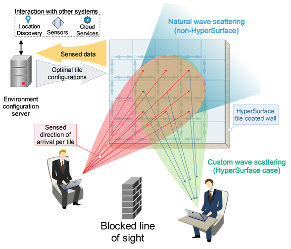
Figure 1: The proposed approach involving HyperSurface tile-coated environmental objects. The wireless propagation is tailored to the needs of the communication link under optimization. Unnatural propagation, such as lens-like focus and negative reflection angles can be provided.

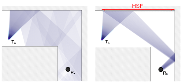
Figure 2: HyperSurfaces (HSF) can counter free space path loss by acting as a lens for impinging waves. A ray tracing-derived showcase with a single transmitter (Tx) / receiver (Rx) pair is shown. Darker colors denote higher signal power levels.

Programming and manipulating the wireless propagation and its effect requires precise sensing of emitted waves in the first place. This can be accomplished by employing external systems [6], such as device localization systems [7], and deduce the nature of their emissions, or by incorporating EM field sensors within HyperSurfaces [8]. While valid, these solutions introduce the complexity of adding new hardware and orchestrating different systems. The present work contributes a wave sensing system for use in intelligent environments that does not have such restrictions. Common signal power level measurements taken by a single antenna/device are shown to suffice for reconstructing the EM wavefront impinging on a HyperSurface, and manipulating it accordingly. Moreover, the same HyperSurface can execute both tasks (i.e., sensing and manipulating waves) at the same time. The methodology follows the principles of compressed sensing and RF single-radar imaging [9, 10]. First, we define a HyperSurface configuration that yields a required functionality, such as wave steering. Then, we define a series of additional configurations that can be employed for RF wavefront sensing, and interleave them via a novel approach.

The remainder of this paper is as follows. Section II provides the necessary background knowledge and surveys related studies. Section III presents the proposed scheme. Evaluation follows in Section IV, and the paper is concluded in Section V.

II Background and related works

In this Section we briefly describe the operating principles of HSFs, as well as the concept of compressed sensing, to a level appropriate for the present work. The reader is also redirected below to related studies for further information on these topics.

II-A HyperSurfaces

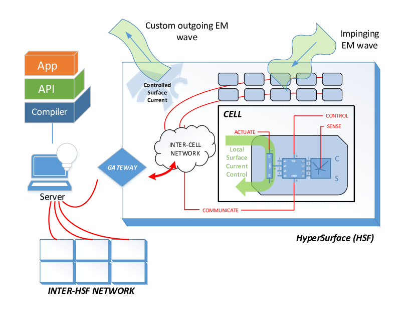
Figure 3: The HyperSurface components, inter-connectivity and operation principles.

The core functionality of HSFs relies on a basic principle in Physics, which states that the EM emissions from a surface are fully defined by the distribution of electrical currents over it. The cause that produces the surface currents are impinging EM waves. Thus, HSFs seek to control and modify the current distribution over them, in order to produce a custom EM emission as a response. This outcome can include any combination of steering, absorbing, polarization and phase alteration and frequency-selective filtering over the original impinging wave, even in ways not found in nature [11].

As shown in Fig. 3, A HSF comprises a massively repeated cell structure (also known as meta-atom), which includes:

• passive conductive elements that can be perceived as receiving/transmitting antennas for the impinging waves,

• an actuation module, which can regulate the local current flow within the cell vicinity (e.g., a simple ON/OFF switch),

• a computation and communication module responsible for controlling the sensory and actuation tasks within the cell, as well as exchange data with other cells (inter-cell networking) to perform synergistic tasks with other cells and communicate with HSF-external entities, and

• optionally, a sensor module to detect the attributes of the impinging wave at the cell vicinity. Notice that the present work does not consider such sensors.

Each HSF unit has a gateway that handles its connectivity to the external word. The gateway participates in the inter-cell network as a peer, and to the external world via any common protocol (e.g., WiFi or Ethernet). Its overall role is to:

• aggregate and transfer sensory data from the HSF to an external controller, and

• receive cell actuation commands and diffuse them for propagation within the inter-cell network.

Finally, a regular computer can act as the external entity that gathers the sensory information from all HSFs within an environment, and subsequently calculates their configurations that fit a given application scenario. For instance, programmable wireless environments use multiple HSFs to customize the wireless propagation for multiple mobile devices, thus achieving state-of-the-art communication quality [6], as conceptually shown in Fig. 1.

HSFs come with software libraries that facilitate the creation of applications. This software suite comprises the HSF Application Programming Interface (API) [12], and the HSF Electromagnetic Compiler [13]. The HSF API contains software descriptions of the metasurface electromagnetic functions and allows the programmer to customize, deploy or retract them on demand via a programming interface with appropriate callbacks. The API serves as a strong layer of abstraction. It hides the internal complexity of the HSF and offers general purpose access to metasurface functions without requiring knowledge of the underlying hardware and physics. The EM Compiler handles the translation of the API callbacks into HSF actuation directives, in an automatic manner, transparently to the user.

Definition 1.

The set of actuation element states corresponding to a given EM functionality (such as wave steering) will be referred to as the HSF configuration for this function.

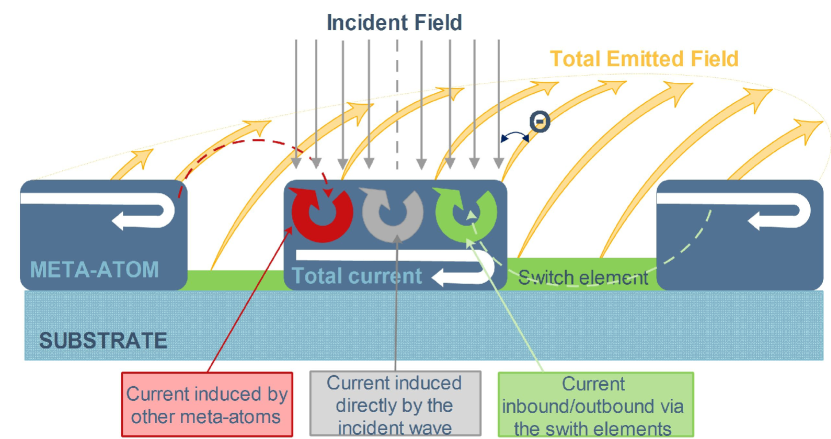
Figure 4: The HyperSurface components, inter-connectivity and operation principles.

One final note on HSFs and metasurfaces in general, is the strong EM interactions between the various cells and components. As shown in Fig. 4, an impinging (incident) EM field creates direct inductive currents to all HSF components. These direct currents also affect each other via induction, and their values stabilize after a transient phase (whose duration is negligible). The states of the switches also affect the current flow distribution, leading to the total outcome (emitted field).

II-B Compressed Sensing

Compressed sensing (CS) is a mathematical tool that can be used to sample a signal below the Nyquist rate, while preserving its reconstruct-ability, without significant loss of precision [14]. CS works on sparse signals, i.e., vectors comprising mostly zeros under some representation.

Let $\boldsymbol{x}$ denote one sparse vector of size $N\times 1$. According to CS, the signal undergoes a sampling process than can be represented by an under-determined linear system:

$${\displaystyle\boldsymbol{o}_{K\times 1}=A_{K\times N}\cdot\boldsymbol{x}{}_{N\times 1}}$$ (1)

where $K<N$. As a rule of a thumb, $K$ is usually in the range of $10\text{\%}-25\text{\%}\cdot N$. The vector $\boldsymbol{o}$ holds the samples or observations of the original vector $\boldsymbol{x}$. The sampling matrix $A$ needs to be uphold some analytical criteria described in [15].

The reconstruction process involves the solution of an under-determined linear system, which is naturally possible only by adding additional restrictions to the solution. In the CS case, the restriction is to minimize the number of non-zero elements of $\boldsymbol{x}$. To this end, a reconstruction process begins with an initial estimate:

$$\boldsymbol{x_{e}^{o}}=A^{T}\cdot\boldsymbol{o}$$ (2)

and proceeds to iteratively “punish” non-zero elements of $\boldsymbol{x_{e}}$, with an overall objective to minimize its $L_{1}$ norm [16], i.e:

$${\displaystyle L_{1}\left(\boldsymbol{x_{e}}\right)=|x_{1}|+|x_{2}|+\dotsb+|x_{n}|.}$$ (3)

The $L_{1}$ minimization objective has been shown to lead to robust and very precise reconstruction outcomes [14]. Existing, free software packages can generate the matrix $A$ and reconstruct the original vector $\boldsymbol{x}$ from the observations $\boldsymbol{o}$ [17].

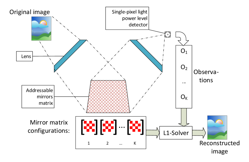
Figure 5: The 1-pixel camera workflow for obtaining visible light images. There is no interaction between the mirror matrix elements, and their reflections are completely independent from each other at the physical layer.

A well-known application of CS is the concept of the single pixel camera [9], whose composition and operation principle is shown in Fig. 5. At the core of this camera there exists an array of micro-mirrors, whose orientation can be individually and programmatically tuned (usually by binary flipping between $\pm 15^{o}$ tilt). An image carried by visible light is sent on this mirror array by means of a simple passive lens. The aggregate reflection outcome is focused on a single photodiode at any given time, again via a standard lens. The $\pm 15^{o}$ mirror tilt is sufficient for sending a single ray on or off the photodiode. By repeating this process several times for different mirror arrangements, one can realize the sampling matrix of a compressed sensing system.

The same principles have been applied to RF imaging, via a concept known in this spectrum as single-radar imaging [10]. In the RF case, the imaging process refers to the reconstruction of the wavefront that reaches a single user antenna. As in the 1-pixel camera, an actuation device similar to the mirror matrix is required, to generate the random multiple-mode modulators required for performing compressed sensing. Programmable metasurfaces have been shown to efficiently fit this role [18, 19, 20]. RF imaging with metasurfaces has been successfully used for approximating the shape of planar metallic objects in space, by emitting waves that impinge upon these objects and then sensing and reconstructing the resulting wavefront [21].

In the present work, we extend the related studies by combining wave manipulation and wavefront sensing at the same time, using the capabilities of HSFs. Thus, the same HSF can sense the direction and attributes of an EM emission from one user device (smartphone, laptop, IoT device), and adaptively steer it toward an access point at the same time [2, 3]. This task is accomplished without adding field sensing hardware to the setup [8].

III Configuring HSFs for joint sensing and wave manipulation

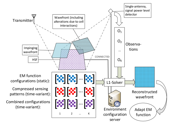
Figure 6: The proposed joint sensing and wave manipulation workflow via HyperSurfaces.

Consider a wireless communication setup illustrated in Fig. 6, comprising a transmitter, a HSF and an environment configuration server. The transmitter seeks to send data to a receiver (which is not shown as it is irrelevant to the setup) while the HSF facilitates this communication according to the programmable wireless environment concept shown in Fig. 1. This can be accomplished by an EM function, e.g., focusing and steering the EM wave impinging on the HSF towards the receiver.

We will denote the HSF configuration that matches the intended EM function as $C_{F}$. As discussed in Section II, $C_{F}$ is a $n\times n$ array, where each element $c_{F}^{ij}$ describes the state of the actuation element inside the HSF cell with indexes $i,j$. Since HSFs with binary (ON/OFF) actuation elements are more tractable to manufacture at low cost and large scales [22], we will focus on configurations with binary elements (i.e., $1$ or $0$). Under normal operation, i.e., without sensing duties, the environment configuration server simply programs the HSF to follow the $C_{F}$, and the required EM function materializes in the environment.

Let us now consider a scenario where the HSF performs wave sensing only, following the RF imaging setup of Fig. 6. The objective is to detect the power of the impinging wave at each of the HSF cells. Following the 1-pixel camera equivalent, the HSF needs to undergo a series of configurations for sensing, denoted as $C_{S}^{k},\,k=1\ldots K$. For each configuration, the server collects the corresponding signal power measurements, $P_{1},P_{2},\ldots P_{K}$, taken from an observing wireless device, denoted as detector in Fig. 6. (Notice that the detector may coincide with the transmitter or the receiver. However, we focus on the general case where the detector is a separate user device). Finally, the server reconstructs the impinging wavefront via the $L_{1}$ minimization process described in Section II-B.

We proceed to study the following issues:

1. How can we transform the CS sampling matrix, $A$, (which is generated by existing software [17]) into the $C_{S}^{k},\,k=1\ldots K$ configurations for the HSF?

2. How can we combine $C_{F}$ with any $C_{S}^{k}$?

For the first issue, notice that the elements of $A$ are real numbers in general [17]. Thus, we will seek to replace each row of $A$ with a number of new rows with binary elements. We generalize this process as a real-vector-to-binary-array decomposition process and formalize it as Algorithm 1.

1

 Input: A vector of reals, $\boldsymbol{v_{1\times N}}$; A number of decimal digits to preserve, $I_{e}$; an acceptable error, $\epsilon$.

2

Output: A binary matrix, $B_{...\times N}$; a vector of reals $\boldsymbol{s}_{1\times...}$; the real constants $S$,$D$,$U$.

3

4 $S\leftarrow\min\left\{\boldsymbol{v}\right\}$;

5

6$D\leftarrow\max\left\{\boldsymbol{v}-S\right\}$;

7

8if D=0 then

9      $B\leftarrow\emptyset_{1\times N}$;

10      $D\leftarrow 1$;

11      $U\leftarrow 1$;

12      $\boldsymbol{s}\leftarrow 1$;

13      $\boldsymbol{return}$;

14 end if

15

16$\boldsymbol{v}\leftarrow round\left(\frac{\boldsymbol{v}}{D}\cdot 10^{I_{e}}\right)$;

17

18$B\leftarrow\emptyset$;

19

20$\boldsymbol{s}\leftarrow\emptyset$;

21

22$\boldsymbol{l}^{prev}\leftarrow\emptyset$;

23

24$coeff\leftarrow 1$;

25

26while $true$ do

27       $\boldsymbol{l}\leftarrow\boldsymbol{v}:v_{i}>0$;

28       if $\frac{\sum\boldsymbol{l}}{N}<\epsilon$ then

29            $return$;

30       end if

31      if $\boldsymbol{l}=\boldsymbol{l}^{prev}$ then

32            $coeff\leftarrow coeff+1$;

33       end if

34      else

35            $\boldsymbol{l}^{prev}=\boldsymbol{l}$;

36            $B.add\_row\left(\boldsymbol{l}\right)$;

37             $\boldsymbol{s}.add\_element\left(coeff\right)$;

38             $coeff\leftarrow 1$;

39       end if

40      $\boldsymbol{v}\leftarrow\boldsymbol{v}-\boldsymbol{l}$;

41      

42 end while

43

 

Algorithm 1 The binary vector decomposition process.

At lines 1-10, the original vector is normalized in the range $\left[0,1\right]$ (including a check for the case of a vector with all-equal elements at line $3$). Subsequently, the normalized vector elements are scaled by a power of $10$, depending on the number of decimal digits that we wish to preserve during the decomposition. Over lines 15-30, the process creates the rows of $B$ by marking the non-zero elements of the scaled $\boldsymbol{v}$ with a binary ’$1$’ flag (line 16), and promptly subtracting it from the scaled vector (line 29). The process terminates if the number of non-zero elements in a new row fall below a user-supplied amount, $\epsilon$ (line 17). Indicatively, as shown later in Section IV, a value of $\epsilon=1\nicefrac{{o}}{{oo}}$ yields no discernible loss on the quality of the sensed outcome. Finally, at lines 20-22 and 27, the process counts how many times a scaled line appears (to avoid row repetitions in $B$), and returns it as a vector $\boldsymbol{s}$. The original vector can be composed from the process outputs as:

$$\boldsymbol{v}\approx\left(\sum_{\forall i}s_{i}\cdot\boldsymbol{B}_{\boldsymbol{row}\left(i\right)}\right)\cdot\frac{D}{U}+S$$ (4)

Going back to equation (1), assume that we treat a row, $\boldsymbol{a}_{i}$, of $A$ as the vector $\boldsymbol{v}$ to be decomposed. Then, a single observation $o_{i}$ is equal to:

$$o_{i}=\boldsymbol{a}_{i}\cdot\boldsymbol{x}\stackrel{{\scriptstyle(\ref{eq:decomp})}}{{\approx}}\left(\sum_{\forall i}s_{i}\cdot\boldsymbol{B}_{\boldsymbol{row}\left(i\right)}\cdot\boldsymbol{x}\right)\cdot\frac{D}{U}+S\cdot\left(\sum_{\forall m}x_{m}\right)$$ (5)

where for future reference we denote the quantity:

$$X=\left(\sum_{\forall m}x_{m}\right)$$ (6)

For the second issue, i.e., of combining $C_{F}$ and $C_{S}^{k}$ configurations, we follow an interleaving approach. First, we define a mask, $\mathcal{M}$, as a binary $n\times n$ array with elements:

$$\mu_{ij}=\left\{\begin{array}[]{c}1,\,\text{iff $i$ and $j$}\text{\,are even,}\\ 0,\,\text{otherwise.}\end{array}\right.$$ (7)

Subsequently, we redefine $C_{S}^{k}$ as a $m\times m$ matrix, where $m=\nicefrac{{n}}{{2}}$ (assuming that $n$ is even, with no loss of generality). In other words, we change our objective to sense the impinging wave only at every other cell, given that this information is still enough to characterize the impinging wave. Then, the combined configuration for EM sensing and manipulation, $C_{S-F}$ is calculated as:

$$C_{S-F}\left(C_{S}^{k},C_{F}\right):C_{F}\left(\mathcal{M}\right)\leftarrow C_{S}^{k},$$ (8)

i.e., the mask is treated as a 2D index for replacing every other element of $C_{F}$ with those of $C_{S}^{k}$.

1

 Input: The HSF side size, $n$ (in number of cells); A sampling matrix, $A_{K\times\left(n^{2}\right)}$; An EM function configuration, $C_{F}$; Decimal digits to preserve, $I_{e}$; Acceptable error, $\epsilon$.

2

Output: The sensed wavefront, $\mathcal{W}$.

3

4 $\mathcal{M}\leftarrow equation\left(\ref{eq:mask}\right)$;

5

6$m\leftarrow\nicefrac{{n}}{{2}}$;

7

8$\boldsymbol{o}\leftarrow\emptyset_{1\times K}$;

9

10$X\leftarrow ObtainMeasurement\left(\mathcal{M}\right)$;

11

12for $i=1\ldots K$ do

13      $\left\{B,\boldsymbol{\text{s}},S,D,U\right\}\leftarrow BinaryDecomposition\left(\boldsymbol{a_{i}},I_{e},\epsilon\right)$;

14      $M\leftarrow 0$;

15      for $each\,row\,\boldsymbol{b_{i}}\,of\,B$ do

16            $C_{s}\leftarrow reshape\left(\boldsymbol{b_{i}},m\times m\right)$;

17             $P\leftarrow ObtainMeasurement\left(\mathcal{C}_{S-F}\left(\mathcal{C}_{S},\mathcal{C}_{F}\right)\right)$;

18            $M\leftarrow M+P\cdot s_{i}$;

19            $o_{i}\leftarrow M\cdot\nicefrac{{D}}{{U}}+S\cdot X$;

20       end for

21      

22 end for

23

24$\boldsymbol{x_{e}}\leftarrow SparseReconstruct\left(\boldsymbol{o},A\right)$;

25

26$\mathcal{W}\leftarrow reshape\left(\boldsymbol{\boldsymbol{x_{e}}},m\times m\right)$;

27

 

Algorithm 2 The joint wave sense-manipulate system operation.

Next, we proceed to formulate the complete system operation as Algorithm 2. At lines 1-3, the process initializes the mask, sets the vector of observations to an empty state, and initializes $m$. At line 4, we perform a special measurement once, to gain an estimate of the quantity $X$ of equation (6). Since $X$ is essentially the sum of all elements of the impinging wave, we perform a measurement with the mask acting as the HSF configuration (i.e., all bits at the cells to be sensed set to ON). At line 6, the process decomposes each row of $A$ via Algorithm 1. Each binary decomposition is reshaped as a $m\times m$ matrix (line 9), gets combined with the $C_{F}$ and deployed to the HSF. A power measurement is obtained, and the observation row is updated per element at line 12, following relation (5). Finally, at line 15-16 the wavefront is reconstructed and reshaped as a $m\times m$ matrix. (Notice that reshaping pertains to splitting a vector into $m$ parts and concatenating them vertically).

IV Evaluation

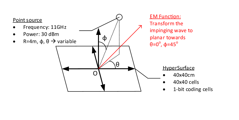
Figure 7: Overview of the evaluation setup.

We proceed to evaluate the proposed scheme using simulations implemented in MATLAB [23].

Setup

We consider the setup of Fig. 7 comprising a HSF with dimensions $40\times 40\,\text{cm}$ and a number of cells equal to $n^{2}=1600$ (i.e, regular $n\times n$ cell layout). Each cell contains one active element (PIN diode) that can be either ON or OFF. Thus, a HSF configuration is a $40\times 40$ array of binary elements. This setup replicates the one proposed by Li et al. in [22]. This study offers an analytical way of:

• Calculating the configuration that matches a required EM function.

• Calculating the scattering diagram of the HSF, for any input configuration.

One additional reason for picking this setup is that the aforementioned analytical models have been validated via real EM measurements [22].

We consider one point source (isotropic) whose electromagnetic attributes are given in Fig. 7. The detector is fixed at $\phi=0^{o}$, $\theta=0^{o}$, $R=4\,\text{m}$. During the experiments, the source will be placed at different points over a sphere with radius $R=4m$ centered at the HSF origin, $O$. Our objective is to reconstruct the HSF-impinging wavefront via compressed sensing, and study its relation to the position of the point source each time.

In all subsequent experiments, the EM function performed by the HSF remains static. The HSF seeks to transform the point source emissions to a planar wave departing towards the direction $\phi=45^{o}$, $\theta=0^{o}$. The mask is also fixed to $m^{2}=400$ pixels (regular $m\times m$ grid). Furthermore, we set $K=300$, $I_{e}=2$ and $\epsilon=10^{-3}$. The software of  [17] is used for creating the sampling matrix and performing the sparse signal reconstruction.

(a) $\phi:20^{o}$,$\theta:0^{o}$

(b) $\phi:20^{o}$,$\theta:45^{o}$

(c) $\phi:20^{o}$,$\theta:90^{o}$

(d) $\phi:40^{o}$,$\theta:0^{o}$

(e) $\phi:40^{o}$,$\theta:45^{o}$

(f) $\phi:40^{o}$,$\theta:90^{o}$

(g) $\phi:60^{o}$,$\theta:0^{o}$

(h) $\phi:60^{o}$,$\theta:45^{o}$

(i) $\phi:0^{o}$,$\theta:0^{o}$

Figure 8: Sensed wavefronts reconstructed via the proposed approach, for various locations ($\phi$,$\theta$) of the point source. The distance of the point source from the origin is fixed to $4\,\text{m}$.

Results

Figure 8 shows the reconstructed wavefronts, for various point source locations. When the source is located directly above the HSF (Fig. 8i), the reconstructed wavefront exhibits an expected circular form, as well as additional, unexpected concentric circles. This effect is due to the interactions among the HSF cells, discussed in the context of Fig 4, which introduce artifacts into the sensed wavefront. Notice that the HSF configuration seeks to transform the incident–spherical–wavefront into a planar one, resulting into complex cross-cell interactions.

As the $\phi$ of the point source position increases (Fig. 8a, 8d, 8g), the concentric pattern is progressively shifted towards the right, following the position of the source. Likewise, when the $\theta$ of the point source location increases (Fig. 8a, 8b, 8c and 8d, 8e, 8f and 8g, 8h), the concentric pattern rotates counter-clockwise, again following the location of the point source.

TABLE I: Effects of wave sensing on the EM manipulation function efficiency.

$\phi$	$\theta$	EM function efficiency	$\frac{n^{2}-m^{2}}{n^{2}}$	$\sigma$ during sensing
$20^{o}$	$0^{o}$	75%	75%	0.00493%
$20^{o}$	$45^{o}$	77%	75%	0.00477%
$20^{o}$	$90^{o}$	73%	75%	0.00470%
$40^{o}$	$0^{o}$	71%	75%	0.00517%
$40^{o}$	$45^{o}$	70%	75%	0.00493%
$40^{o}$	$90^{o}$	70%	75%	0.00454%
$60^{o}$	$0^{o}$	70%	75%	0.00453%
$60^{o}$	$45^{o}$	67%	75%	0.00487%
$0^{o}$	$0^{o}$	89%	75%	0.00609%

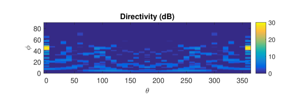
(a) Scattering diagram of the HSF for no sensing.

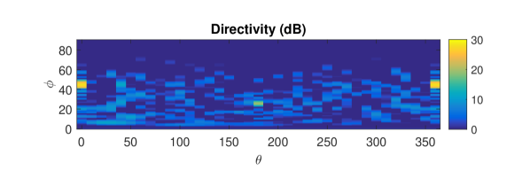
(b) The same scattering diagram with sensing enabled.

Figure 9: Indicative effects of sensing on the scattering pattern of the HSF for a given EM function ($\phi:0$, $\theta:0$).

We proceed to study the effects of combining wave sensing with the EM function to the efficiency of the latter. To this end, we execute one simulation with pure EM functionality without combined sensing and we log the power, $P_{max}$, reflected towards the intended direction ($\phi:45^{o}$,$\theta:0$). Then, for each of the cases showed in Fig. 8 (which include sensing), we execute the same run and log the power reflected towards the same direction, $P$. The ratio $\nicefrac{{P}}{{P_{max}}}$ is the EM function efficiency column in Table I. Notably, the efficiency is very close to the ratio $\nicefrac{{n^{2}-m^{2}}}{{n^{2}}}$, which represents the configuration array elements assigned to the EM function, after subtracting the ones assigned to sensing. The EM function efficiency when combined with sensing is thus approximately $75$%. Variations around this value are owed to the fact that sensing and wave manipulation configurations can be occasionally aligned to each other (leading to higher efficiency) or incompatible (leading to lower efficiency). Additionally, we log the standard deviation of the EM function efficiency over all sampling observations, and conclude that it is negligible as shown in Table I. In other words, the effects of sensing on an EM function are static with regard to the sensing configurations employed.

Finally, in Fig. 9 we proceed to study the effects of sensing on the whole HSF scattering diagram for one indicative case (point source at $\phi:0$, $\theta:0$). Figure 9a shows the scattering pattern when no sensing is employed, which naturally contains parasitic lobes across which we have approximately $20\,\text{dB}$ lower power than the main lobe facing towards the intended direction ($\phi:45^{o}$, $\theta:0$). The effects of introducing sensing are shown in Fig. 9b. While the addition of sensing duties introduces some additional parasitic lobes, they remain much below the power of the main lobe, with a $15-20\,\text{dB}$ difference.

Discussion and future directions

Programmable wireless environments promise full manipulation of EM propagation in the form of wave "routing", i.e., hopping from tile to tile while performing beam focusing [2, 3, 4]: i) to maximize the power transferred to a remote device, either for tele-charging or better quality of communication, ii) to minimize the power received by a set of unintended devices, either for eavesdropping mitigation or for interference cancellation. Additional applications include: i) the mitigation of Doppler effects by ensuring that EM waves are received from a direction perpendicular to the movement trajectory of the receiver, and ii) EM wave scrambling and unscrambling via destructive and constructive phase modification for advanced security during the propagation via unsafe spaces [6].

In the present work, we studied a crucial requirement for enabling these applications, i.e., the sensing of the EM wavefront that impinges upon a tile. The proposed joint wave sensing and wave manipulation was shown to extract useful information that strongly correlates with the position of the point source. Moreover, the effects of the sense/manipulate combination on the intended EM function can be manageable, as they do not alter the HSF scattering pattern significantly. The combination introduces a drop in efficiency of the EM function that is dictated by the number of HSF cells assigned to sensing duties. This efficiency drop can thus be minimized in HSFs with many cells in total, while keeping the number of sensing cells constant.

In practical terms, the presented scheme can be deployed in two ways. First, a receiving device can also act as the detector of the compressed sensing process. In this case, the receiver can obtains incoming power measurements and send them to the environment configuration server for processing. The second way employs dedicated detectors placed at few fixed points within the environment. Using beam-forming, they can target tiles, obtained power measurements and send them to the server for processing.

In the future, the sensed wavefronts will be processed via machine learning techniques, to filter out the effects of the cell cross-interactions and yield accurate wavefront measurements. Such measurements can then be used for adaptively fine-tuning the HSF functions, to the benefit of wireless devices. Moreover, the source sensing outcomes of the proposed approach can be combined with external sensing systems to improve their overall efficiency.

V Conclusion

Programmable metasurfaces are the enablers of the Internet of Material Properties, by introducing smart planar materials–the HyperSurfaces–that can interact with impinging electromagnetic waves in a software defined, adaptive manner. Highly promising applications include the programmable wireless environments, wherein the electromagnetic propagation is programmable, allowing for wave routing and introducing novel capabilities in communication performance, security and power transfer. Central to this paradigm is the sensing of waves that impinge upon a HyperSurface, which typically rely on sensory hardware either internal or external to the surface. The present work introduces a wave sensing that does not employ hardware. Instead, it programs the HyperSurface in a manner that interleaves a required electromagnetic behavior with a compressed sensing workflow. The work showed that the impinging wave can be reconstructed by simple power measurements at a single observation point, without significantly affecting the desired electromagnetic behavior of the HyperSurface.

References

- [1] I. F. Akyildiz, S. Nie, S.-C. Lin, and M. Chandrasekaran, “5g roadmap: 10 key enabling technologies,” Computer Networks, vol. 106, pp. 17–48, 2016.
- [2] C. Liaskos, A. Tsioliaridou, A. Pitsillides, S. Ioannidis, and I. F. Akyildiz, “Using any Surface to Realize a New Paradigm for Wireless Communications,” Communications of the ACM, vol. 61, pp. 30–33, 2018.
- [3] ——, “A New Wireless Communication Paradigm through Software-controlled Metasurfaces,” IEEE Communication Magazine, vol. 56, no. 9, pp. 162–169, 2018.
- [4] ——, “Realizing Wireless Communication through Software-defined HyperSurface Environments,” in WoWMoM 2018, June 12-15, Chania, Crete, Greece, pp. 1–10.
- [5] O. Tsilipakos, A. C. Tasolamprou, T. Koschny, M. Kafesaki, E. N. Economou, and C. M. Soukoulis, “Pairing toroidal and magnetic dipole resonances in elliptic dielectric rod metasurfaces for reconfigurable wavefront manipulation in reflection,” Advanced Optical Materials, vol. 6, no. 22, p. 1800633, 2018.
- [6] C. Liaskos, N. Shuai, A. Tsioliaridou, A. Pitsillides, S. Ioannidis, and I. Akyildiz, “A novel communication paradigm for high capacity and security via programmable indoor wireless environments in next generation wireless systems,” Ad Hoc Networks, vol. 87, pp. 1–16, may 2019.
- [7] S. Shi, S. Sigg, L. Chen, and Y. Ji, “Accurate location tracking from csi-based passive device-free probabilistic fingerprinting,” IEEE Transactions on Vehicular Technology, vol. 67, no. 6, pp. 5217–5230, 2018.
- [8] A. Tsioliaridou, C. Liaskos, A. Pitsillides, and S. Ioannidis, “A Novel Protocol for Network-controlled Metasurfaces,” in ACM NANOCOM’17, pp. 3:1–3:6.
- [9] M. F. Duarte, M. A. Davenport, D. Takhar, J. N. Laska, T. Sun, K. F. Kelly, and R. G. Baraniuk, “Single-pixel imaging via compressive sampling,” IEEE signal processing magazine, vol. 25, no. 2, pp. 83–91, 2008.
- [10] H. B. Wallace, “Analysis of rf imaging applications at frequencies over 100 ghz,” Applied optics, vol. 49, no. 19, pp. E38–E47, 2010.
- [11] A. Li, S. Singh, and D. Sievenpiper, “Metasurfaces and their applications,” Nanophotonics, vol. 7, no. 6, pp. 989–1011, jun 2018.
- [12] C. Liaskos, A. Tsioliaridou et al., “Initial UML definition of the HyperSurface programming interface and virtual functions,” European Commission, H2020-FETOPEN-2016-2017, Project VISORSURF: Accepted Public Deliverable D2.1, 31-Dec-2017, [Online:] http://www.visorsurf.eu/m/VISORSURF-D2.1.pdf, 2017.
- [13] C. Liaskos, A. Pitilakis et al., “Initial UML definition of the HyperSurface compiler middle-ware,” European Commission, H2020-FETOPEN-2016-2017, Project VISORSURF: Accepted Public Deliverable D2.2, 31-Dec-2017, [Online:] http://www.visorsurf.eu/m/VISORSURF-D2.2.pdf, 2017.
- [14] D. L. Donoho et al., “Compressed sensing,” IEEE Transactions on information theory, vol. 52, no. 4, pp. 1289–1306, 2006.
- [15] E. J. Candès and M. B. Wakin, “An introduction to compressive sampling [a sensing/sampling paradigm that goes against the common knowledge in data acquisition],” IEEE signal processing magazine, vol. 25, no. 2, pp. 21–30, 2008.
- [16] Y. Tsaig and D. L. Donoho, “Extensions of compressed sensing,” Signal processing, vol. 86, no. 3, pp. 549–571, 2006.
- [17] E. Brad. [Online]. Available: https://statweb.stanford.edu/ candes/l1magic/
- [18] W. L. Chan, H.-T. Chen, A. J. Taylor, I. Brener, M. J. Cich, and D. M. Mittleman, “A spatial light modulator for terahertz beams,” Applied Physics Letters, vol. 94, no. 21, p. 213511, 2009.
- [19] C. M. Watts, X. Liu, and W. J. Padilla, “Metamaterial electromagnetic wave absorbers,” Advanced materials, vol. 24, no. 23, pp. OP98–OP120, 2012.
- [20] B. Sensale-Rodriguez, S. Rafique, R. Yan, M. Zhu, V. Protasenko, D. Jena, L. Liu, and H. G. Xing, “Terahertz imaging employing graphene modulator arrays,” Optics express, vol. 21, no. 2, pp. 2324–2330, 2013.
- [21] Y. B. Li, L. L. Li, B. B. Xu, W. Wu, R. Y. Wu, X. Wan, Q. Cheng, and T. J. Cui, “Transmission-type 2-bit programmable metasurface for single-sensor and single-frequency microwave imaging,” Scientific reports, vol. 6, p. 23731, 2016.
- [22] H. Yang, X. Cao, F. Yang, J. Gao, S. Xu, M. Li, X. Chen, Y. Zhao, Y. Zheng, and S. Li, “A programmable metasurface with dynamic polarization, scattering and focusing control,” Scientific reports, vol. 6, p. 35692, 2016.
- [23] MATLAB, version R2015. Natick, Massachusetts: The MathWorks Inc., 2015.