Volume uncertainty assessment method of asteroid models from disk-integrated visual photometry.

Abstract

The need for more accurate asteroid models is perhaps secondary to the need to measure their quality. The uncertainties of models’ parameters propagate to quantities like volume or density – the most important and informative properties of asteroids – affecting conclusions about their physical nature. Our knowledge on shapes and spins of small solar system bodies comes mostly from visual, disk-integrated photometry. In this work we present a method for asteroid model uncertainty assessment based on visual photometry (lightcurves and sparse-in-time absolute measurements) allowing the determination of realistic volume uncertainty, as well as spin axis orientation, rotational period and local surface features. The sensitivity analysis is conducted by creating clones of the nominal model and accepting the ones that fit the observations within a confidence level. The uncertainties of model parameters are extracted from the extreme values found in the accepted clone population. Creation of such population of clones enables the conversion of a deterministic asteroid model into stochastic one, and can be utilized to create observation predictions with error bars. The method was used to assess the uncertainties of fictitious test models and real targets, i.e. (21) Lutetia, (89) Julia, (243) Ida, (433) Eros and (162173) Ryugu. We conclude that volumes, and subsequently, densities of asteroids derived from lightcurve-based models likely have vastly understated uncertainties, the biggest source of which is the inability to establish the extent of the model along its spin axis.

1 Introduction

Volume is one of the most important physical parameters of asteroids. When combined with the mass estimate, it is essential in the bulk density determination; which, in turn, allows us to peek inside asteroids and make conclusions about their inner structure, like the macro and micro porosity, chemical composition or material differentiation (Scheeres et al., 2015). Volume can be the result of scaling of an asteroid shape model with absolute measurements or a technique based on them, e.g. stellar occultations (e.g., Ďurech et al. (2011)), adaptive optics images (e.g., Hanuš et al. (2013a)) or thermophysical modelling (e.g., Usui et al. (2011), Hanuš et al. (2015), Alí-Lagoa et al. (2018), Marciniak et al. (2018)). The shape models can vary from spheres, 3-axial ellipsoids through convex to non-convex shapes, they can be established via different methods and based on single (Kaasalainen et al., 2001; Bartczak & Dudziński, 2018) or multiple data types at once (Carry et al., 2010a; Viikinkoski et al., 2015; Ďurech et al., 2017). The latter results in model that explains different datasets simultaneously rather than being simply scaled, which is a great advantage of multi-dataset inversion. Although limited to a small number of targets, it provides valuable and detailed information about them (Carry et al., 2008; Berthier et al., 2014; Pajuelo et al., 2018; Vernazza et al., 2018).

Though we have seen tremendous advances in shape and spin modelling techniques throughout decades, the problem of quantitative quality assessment of asteroid models from disk-integrated photometry, without the presence of auxiliary data to compare to, remains untackled. In case of lightcurve-only based models, the uncertainty of volume – when reported – comes only from the precision of supplemental data (e.g. time resolution of stellar occultation timings) used for scaling the shape models. However, the uncertainty of the shape model parameters, i.e. vertices describing the shape, spin axis orientation or rotational phase, influence such fits as well. The shape model uncertainty propagates to volume and, analogously, to any other property determined from the shape model, affecting conclusions drawn for the population of small bodies under scrutiny. Even when no absolute measurements are available and size cannot be determined in physical units, dimensionless volume and shape model parameters uncertainties are of much value in models’ quality assessment.

There definitely is a compelling need for a procedure of quality and uncertainty assessment of asteroid models. Without it, we are not able to compare the models and decide which is better or worse. What is more, we cannot express our doubts about the models in numerical values, leaving us with vague qualitative estimates only. Models’ fit to the data, e.g. expressed in $\chi^{2}$ of the fit, is insufficient to test their robustness. To give a simple example, a spherical body can be modelled equally well with any spin axis orientation, leaving these parameters totally uncertain. Similarly, some shape parameters can also be unconstrained by observational dataset, meaning we do not have the means to tell which parameters can be trusted and which are simply the artefacts of the method used. For instance, if we observe a body only from one viewing angle, its far side can either stretch far back or be concave. Flattening or thickening of a shape model would again not be detected in relative photometric lightcurves. This has a huge effect on the volume determination and currently we are not equipped well enough to account for that. Additionally, some inescapable factors affect the models as well, like data precision, human error, assumptions (e.g. homogeneous albedo or mass distribution, principal axis rotation), simplifications of underlying physics (e.g. using simplistic light scattering law) and approximations, to name a few.

By far, the most abundant data type for the most numerous target sample is disc-integrated photometry in visual bands and the majority of published asteroid shape models are based solely on it. The Asteroid Lightcurve Photometry Database (Warner et al., 2009), as of October 2018, contains lightcurve observations for 13578 objects. In contrast, only hundreds of shape models were obtained using other techniques. Accordingly, as a first step, we focused on creating a method for asteroid shape models’ uncertainty assessment based on, and in regard to, this type of data. The method is not designed to search for new, better, global minimum, although some models with better fit are found during the process. Due to the overwhelmingly large amount of parameters and possible geometries it is impossible to scan the whole parameter space. Finding a model that fits observations is a job for a modelling technique, whichever used. The presented method explores only the proximity of the nominal solution and is based on creating clones of the tested model. The main goal is to obtain relative, dimensionless volume uncertainty and to expose parameters’ indeterminacy caused by light variation to shape mapping and incompleteness of observational dataset.

In section 2 we take a quick look at available procedures commonly used to evaluate the models. In section 3 we analyse the limits of volume accuracy due to observing geometries, and information content of relative lightcurves and absolute photometry, i.e. the ability to establish models’ scale along their spin axis. Next (Sec. 4), we describe the method of asteroid shape model uncertainty assessment, giving synthetic example in section 6 followed by an evaluation of five real targets in section 7.

2 Available quality assessment procedures

The term asteroid model, or just model, used hereafter denotes a set of parameters describing the shape, spin axis orientation, rotational period, phase of rotation for reference epoch and scattering law used to reflect light of the surface. Due to the lack of standard procedures of quality assessment regarding asteroid models there is no publicly available information on models’ uncertainties, except for arbitrary in-house quality codes. Researchers, when using models in their studies, must resort to experts’ opinion, each probably based on different criteria for model evaluation. There is a valid question of subjectivity of such assessments, as well and the problem with the choice of judges (see Uusitalo et al. (2015) and references therein). In this section we take a quick look at the frequently used approaches to the problem.

There is a common notion of three or four apparitions being sufficient to create decent models (Kaasalainen et al., 2002b). The models are indeed often judged by the number of apparitions and lightcurves used during the modelling. There is no doubt that the quality and quantity of data used in modelling (e.g. signal to noise ratio, number of lightcurves, number of points per lightcurve, the distribution of apparitions entangled with spin axis orientation that define geometries under which an asteroid was observed, etc.) have major influence on the outcomes. However, each target is unique and poses different challenges. For example, if the rotational axis’ latitude is near $\pm 90^{\circ}$ every lightcurve carries the same information, so neither the number of them, nor the number of apparitions matter shape-wise. The situation presents itself totally different for latitudes near $0^{\circ}$. There cannot be a universal set of rules to follow when observing an asteroid to guarantee a good model, as the knowledge of the very physical parameters we are trying to find influences our judgement. One is certain: the more top-quality data available, the better chances we have of creating reliable models.

Another way of model quality assessment one might use would be transferring the robustness measure (whichever one sees fit to use) of the method used in the modeling onto the model itself. The reasoning here is, that if the technique worked for some targets it should work for others as well. There are a few asteroids for which we have complete set of observations regarding shape, size and spin axis orientation – the ones visited by spacecraft probes. One example found in literature is the comparison between the topographic model of (951) Gaspra based on Galileo mission flyby data with lightcurve based one (Kaasalainen et al., 2002a). Another example is the comparison of in situ model of (21) Lutetia with its lightcurve and adaptive optics-based model (Carry et al., 2012), although the evaluation was only possible for a half of the body’s true shape observed by ESA Rosetta spacecraft during 2010 flyby. Also, Bartczak & Dudziński (2018) compare lightcurve based model of (433) Eros to its true shape based on data from NEAR Shoemaker probe.

In both cases model comparisons were used to validate modelling techniques rather than to produce model parameters’ uncertainties which reflect information content of the datasets. Asteroids visited by probes constitute tremendously valuable but tiny sample compared to the number of known targets out there limiting considerably our ability to test methods.

Previous point brings us to another approach, which is making laboratory measurements (Barucci et al., 1982; Barucci & Fulchignoni, 1982; D’Ambrosio et al., 1985) or creating fictitious digital targets and trying to model them from synthetic set of observations (Kaasalainen & Torppa, 2001; Kaasalainen et al., 2005; Bartczak & Dudziński, 2018). Still, it would take tremendous amount of time to test a significant number of targets with large spectrum of possible scenarios (orbits, data quality, rotational phase and phase angle coverage, and surface characteristics defining how light scatters) to be able to review methods in full. Modelling techniques are becoming increasingly complex taking advantage of multiple data types and sophisticated algorithms which hampers spotting limitations and drawbacks of the methods even further.

An analysis of a family of solutions acquired from many modelling runs for a given target can give some insight into the robustness of a model. An extreme, but informative, case would be the modelling of a spherical body or a flattened sphere. No matter which orientation of the rotational axis was chosen, the resulting model would fit the data perfectly indicating insufficient information content in the dataset. The family of solutions is often the basis for accepting or rejecting a model by comparing it with the rest within some confidence level of the fit. A common practice, based on convex inversion method creators’ experience, is to compare the models with the $\chi^{2}$ up to the smallest one enlarged by 5% to 10% (Torppa et al., 2003). This approach is hard to standardize, and does not yield results that allow for comparison of the models of different targets or models from different modelling techniques. Uniform scanning of parameter space near the best solution is also not utilized here, not to mention that these models still carry all of the method-specific problems and assumptions. The behavior or outcome of modelling can provide additional insight and indicate the presence of a very wide global minimum or plethora of local ones, manifesting as dissimilarity of the shapes from family of solutions and/or large scatter of spin axis orientations giving solutions with similar $\chi^{2}$.

Observational techniques other than disk-integrated photometry, even when not used during the modelling, can be valuable for model confirmation and for disambiguation of mirror solutions, e.g. Ďurech et al. (2011); Hanuš et al. (2015). Of course, each technique has its own limitations that need to be understood and taken into account. Especially, when a technique offers only 2D projections of 3D shapes which, depending on the number of available projections, can seriously limit the ability to test the models.

3 Model scale along the spin axis

In this section we take a closer look at the ability to detect the extent of the model along the spin axis due to observing geometries, and shape to scattered light transformation, causing huge volume uncertainty. As stated before, the vast majority of asteroid models are created from relative photometric lightcurves alone, and those are extremely susceptible to this problem. Demonstrating this, a 3-axial ellipsoid models established using amplitudes method alone would have only $a/b$ ratio determined, with $b/c$ unknown and one would needs to utilise differences in absolute magnitudes to assess $b/c$ ratio (Magnusson et al., 1989). Assuming that the models are defined so that spin- and $z$- axes are the same, the term z-scale used hereafter will refer to the extent of a model along the spin axis.

Although the effect of changing the z-scale is most apparent in absolute magnitudes, it also changes the shape and amplitude of the lightcurves in some favorable orientations, therefore one might argue that more advanced methods taking into account all the features of the lightcurves can detect the z-scale with success. As we will show, the observations have to be made for particular epochs (which are target-specific) and with good photometric precision so that the differences (rather small in general) are even detectable.

To illustrate this phenomenon we calculated the average difference between the lightcurves of two 3-axial ellipsoids with the same $a/b=1.25$, but different $b/c$ of $1$ and $2$ (Fig. 1, top). The synthetic observations were made for various longitudes $\lambda_{obs}$ simulating constant observations on the orbit. The observer was put in the position of the light source observing the body always in opposition. The orbit was coplanar with the $xy$ plane of the coordinate system, and the Lommel-Seeliger scattering law was utilized. We repeated this exercise for the model of (9)Metis from Bartczak & Dudziński (2018) by scaling it in $z$-axis by 0.66 and 1.33 (Fig. 1, bottom) and using the same observational setup as for ellipsoids. The volume of the larger ellipsoid ($b/c=1$) is twice the volume of the smaller one ($b/c=2$). The same holds for the two Metis models. It is important to realize that even huge difference in volume results in very little difference in lightcurves even for favorable geometries. The targets would have to be observed at specific $\lambda_{obs}$ for the observer to spot the difference and the chances to do so vary depending on the inclination of the rotational axis. Due to the shape and orientations of the orbits of the Earth and the target, and their orbital periods limited geometries are feasible during apparitions in reasonable time span imposing further constrains. In our examples the biggest possible average difference was $0.02$ mag for the ellipsoids and $0.04$ mag for the (9) Metis models, which is very small compared to the precision of available photometric lightcurves, which typically is $0.01$ mag. All models based solely on relative photometry are affected by this problem, but the extent of the volume uncertainty is case-specific for every target and set of observations.

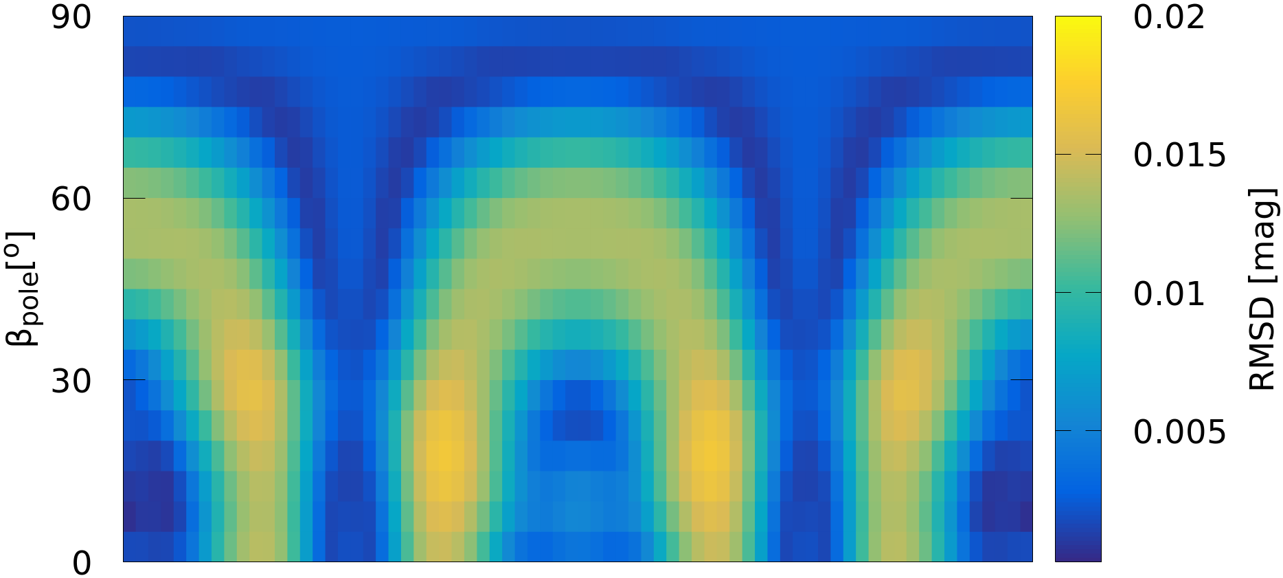
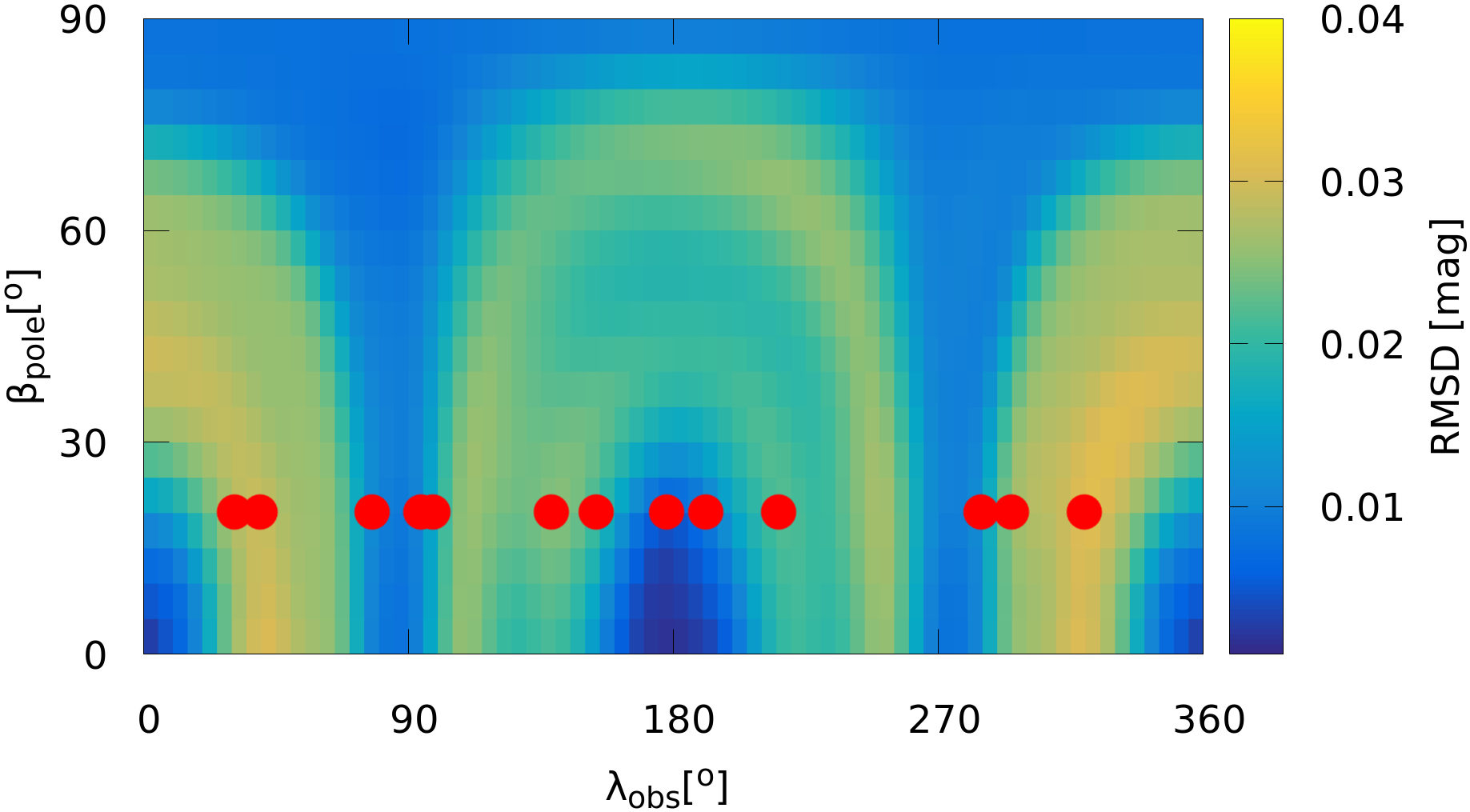
Figure 1: Plot showing average difference of lightcurves of 3-axial ellipsoid with $a/b=1.25$, $b/c=1$ against $b/c=2$ (top) and two (9) Metis (Bartczak & Dudziński, 2018) models scaled in z-axis by 0.66 and 1.33 (bottom). Models were observed at different ecliptic longitudes $\lambda_{obs}$ from $0^{\circ}$ to $360^{\circ}$ at opposition with various pole latitudes $\beta_{pole}$ and Lommel-Seeliger scattering law. Red dots in the bottom plot show observed longitudes of (9) Metis for spin axis $\beta_{pole}=20^{\circ}$. See text for more details.

3.1 Absolute photometry to the rescue

In theory, absolute observations contain information on the extent of an asteroid along the spin axis. In the simple case of 3-axial ellipsoid, the absolute flux $\Phi$ changes as a function of aspect angle $\xi$ – the angle between the rotation axis and asteroid-observer direction. The more $\beta_{pole}$ approaches $0^{\circ}$ the more evident the effect is, as $\xi$ variability increases. The ratio of the model’s semi-axes $b/c$ can be found using magnitudes method, when observations show the difference in brightness depending on the aspect $\xi$, i.e. the change in observed projections with exposed $a$ and $b$ axes in one apparition and $a$ and $c$ axes in the other. This method’s usefulness faints as observed aspect angles’ range decreases and fails completely for $\beta_{pole}$ approaching $\pm 90^{\circ}$ on orbits coplanar with the ecliptic.

Adopting the formalism used by Zappala (1981) we can draw some conclusions about the whole population of asteroids and our ability to determine their volumes. Simple example from previous paragraph hints that this ability depends on available aspect angles under which target can be observed. Assuming a 3-axial ellipsoid described by semi-axes $a$, $b$ and $c$ and with semi-axis $c$ equal to $1$ by definition, the difference in magnitude between two observations taken at aspects $\xi=90^{\circ}$ (equator on) and $\xi$ is

$$\Delta M=M(90^{\circ})-M(\xi)=2.5\log d,$$ (1)

where

$$d=\sqrt{b^{2}\cos^{2}(\xi)+\sin^{2}(\xi)}$$ (2)

is a projection area of the ellipsoid for a given aspect $\xi$.

Fig. 2 illustrates this dependency for different values of semi-axis $b$. Observation at aspect $\xi=90^{\circ}$ can be in principle obtained for every asteroid, regardless of the spin axis latitude $\beta_{pole}$ if we neglect the asteroid orbit’s longitude of ascending node $\Omega$ and spin axis longitude $\lambda_{pole}$. The red dots in Fig. 2 show a difference in magnitudes from photometric measurements with magnitude precision (represented by error bars) of $\delta m=0.1$, which is a typical precision of majority of available sparse-in-time absolute photometry from automated surveys (Hanuš et al., 2011). The non-zero precision in magnitude creates ambiguity in calculated $b$ parameter, i.e. the true $b$ can be confused with different one which leads to ambiguity in volume. In case of 3-axial ellipsoid the change in $b$ causes the same change in the volume of the body. If we assume that the $b$ parameter of an ellipsoid can be derived from the difference $\Delta M$, we are able to estimate, roughly, the uncertainty of the volume for a given target observed at $\xi=90^{\circ}$ and minimal achievable aspect angle $\xi_{\text{min}}$. This can be expressed by the equality:

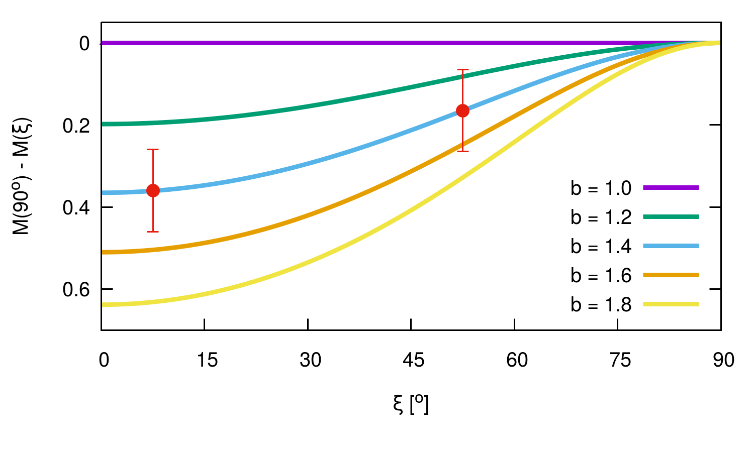
Figure 2: The plot of difference in magnitudes (Eq. 1) versus aspect angle $\xi$ for different values of semi-axis $b$. The semi axis $c=1$ by definition. The red dots show difference in magnitudes from photometric measurements with magnitude precision $\delta m=0.1$, a tipical precision from surveys (Hanuš et al., 2011). The expected precision of upcoming Gaia measurements of $0.001$ mag (Mignard et al., 2007) is about the size of the points.

$$2.5\log d\pm\delta m=2.5\log d^{\prime},$$ (3)

and solving it for $b^{\prime}$ we get

$$b^{\prime 2}_{\pm}=b^{2}\cdot 10^{\pm 0.8\delta m}+(10^{\pm 0.8\delta m}-1)\tan^{2}(\xi).$$ (4)

Now, we are able to calculate the relative uncertainty of volume

$$U(V)/V=\frac{b^{\prime}_{+}+b^{\prime}_{-}}{b}$$ (5)

Fig. 3 shows the relative volume uncertainty $U(V)/V$ for $b=1.2$ and $\delta m=0.1$, $0.05$, $0.01$ and $0.001$ (colour lines) and the cumulative fraction of asteroids (gray bars) for which minimal observable aspect angle $\xi_{\text{min}}$ is achievable. Aspect angles were normalized to $[0^{\circ},90^{\circ}]$ range because of the symmetry of ellipsoidal model. The distribution of spin axis orientations was taken from Asteroid Spin Vectors database (Kryszczyńska et al., 2007). It has to be stressed that the population of models and estimates used to derive those spin properties is biased (Marciniak et al., 2015) and so are the results of our evaluation. Together with the information on the orbits’ inclinations the minimal achievable aspects were calculated neglecting the longitude of spin axis orientations $\lambda_{pole}$ and the orbits longitudes of ascending node $\Omega$.

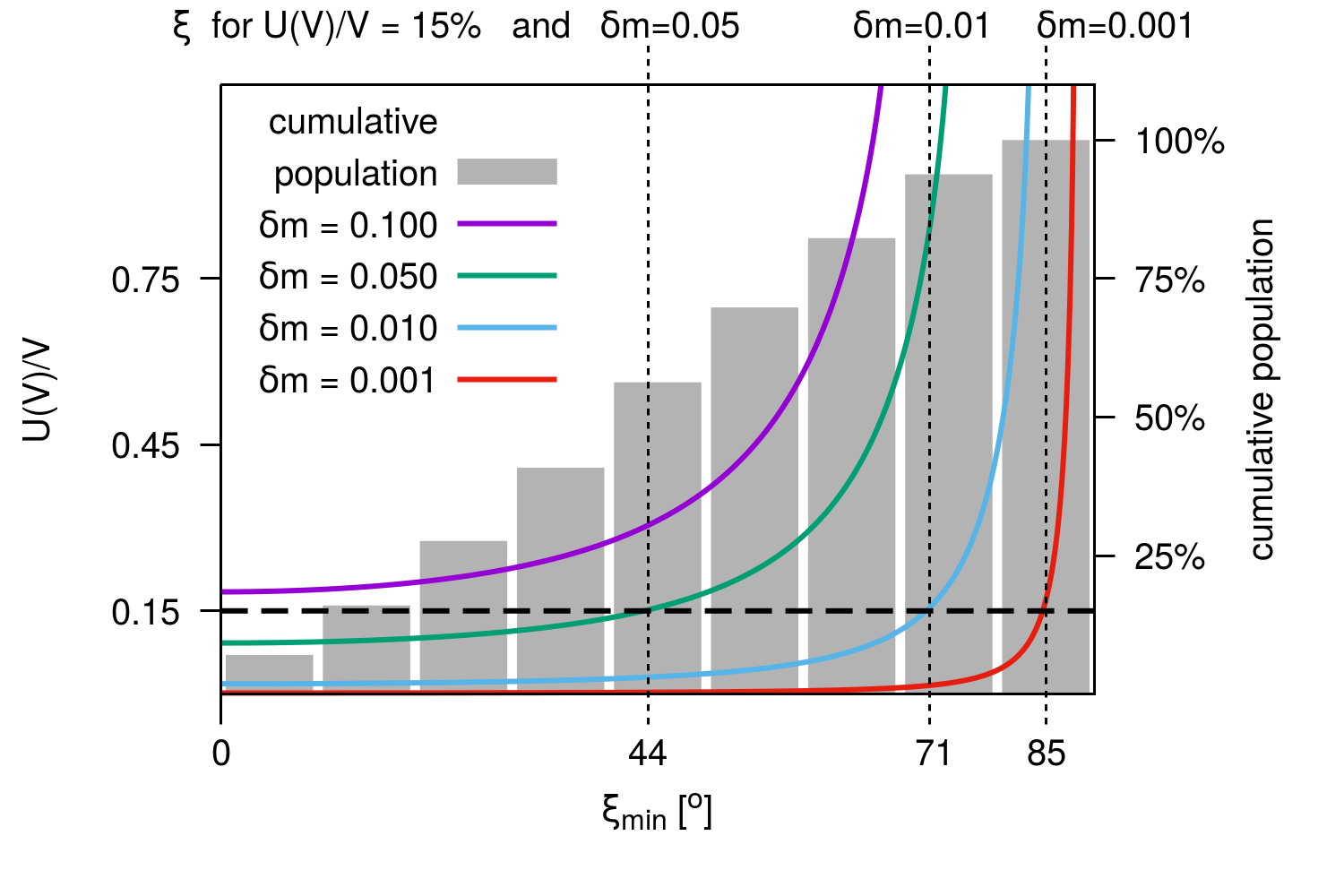
Figure 3: Relative volume uncertainty $U(V)/V$ for minimal observable aspect $\xi_{\text{min}}$ (colour lines) and the cumulative population of asteroids (gray bars) for which this is achievable. The black dashed horizontal line shows 15% level of volume uncertainty. See text for detailed description.

As pointed out by Carry (2012), when mass of an asteroid is known precisely (i.e. relative precision better than 20%) the size estimate is the limiting factor on the density assessment; the models’ volume uncertainties below 10-15% are needed to exploit any mass determination. Assuming said volume accuracy, we can calculate minimal required aspect $\xi_{\text{min}}$ (dashed vertical lines in Fig. 3) below which it is feasible. It further allows us to estimate the fraction of asteroid population for which this is doable. For magnitude precision $\delta m=0.1$ this fraction is 0. When we increase the accuracy to $\delta m=0.05$ the fraction is enlarged to 48% of the population with $44^{\circ}$ minimal aspect angle required, while with $\delta m=0.01$ it is 88% at $71^{\circ}$ aspect angle. For $\delta m=0.001$ volume uncertainty below 15% can be achieved for almost all targets. Such accuracy will be feasible for a fraction of asteroid population using the Gaia observations (Mignard et al., 2007). The outcome, however, depends on the plethora of factors and is therefore target-specific (Spoto et al., 2018).

It is worth remembering that this estimate is rough, but very informative, as it shows the restrictions coming from observing geometries, i.e. what is the best we can hope for. Absolute observations are usually sparse-in-time. Imprecise rotational period estimates leading to big uncertainties in rotational phase for a given time, and low precision in magnitude can pose problems as well when comparing the model to the data. The need for good quality observations is obvious and we all look forward to getting the precise measurements, like the ones Gaia mission will provide. Other techniques offering absolute measurements of the size of a body, i.e. stellar occultation chords and adaptive optics images, could also be used to properly scale the model in z-axis. However, the geometry of such measurements needs to be favorable as well, meaning the aspect of an asteroid needs to be close to $90^{\circ}$. The number of observations utilizing such techniques is still very low (an order of magnitude lower compared to lightcurves).

4 Uncertainty Assessment Method

The main goal of the method presented in this section is to convert a deterministic asteroid model into stochastic one through sensitivity analysis. This modelling-technique independent method is based on creating clones of a nominal model, introducing changes to its parameters and accepting or rejecting them based on how they fit the observations. Uncertainties of model parameters’ are derived from per parameter ranges of values found in accepted clone population. The population of clones inside the confidence level can subsequently be used to create predictions of observations with probability associated with simulated data point rather than single value. Only disk-integrated photometry is considered in this work. The scattering law used to create synthetic lightcurves is the same as the one used during the modelling.

Although rotational period, phase of rotation for reference epoch and scattering law are explicitly defined, the shape parameters describing the same surface can be defined in many ways, e.g. voxels, spherical harmonics, etc. Each representation can be translated to a surface composed of triangular facets defined on a mesh of vertices in 3D space and this scheme is used throughout this work.

4.1 Remesh

There are many ways to represent and change 3D shapes and surfaces. Meshes of vertices and triangular facets defined on them are primarily used in computer graphics and also in asteroid shape modelling. When dealing with models from different asteroid modelling methods the need for unifying the shape representation arises. Making small, uniform changes in models’ parameters is the key component of the method described in this work, and to assure uniformity in model’s shape changes (guaranteeing good statistics), vertices need to be evenly distributed. That also requires consistent triangle sizes, lack of spike-like or huge ones. After remeshing resulting shape stays the same (and gives the same lightcurves, which is of our main concern here), but is much easier to work with (Fig. 4).

The new mesh is achieved by calculating intersection points between model’s surface and equally distributed set of rays originating in the model’s centre. The nature of surface fluctuation creation and their application to the model (see Sec. 4.3) require even mesh, no matter the shape. To get satisfactory level of triangle shapes and sizes uniformity sufficiently big number of rays is used. To construct the set of rays we start with the largest platonic solid consisting of 12 vertices and then use surface subdivision algorithm (Catmull & Clark, 1978) to get bigger and uniform meshes. After 2 iterations we get 242 vertices, and 3842 after 2 more. Triangular facets are well defined on such mesh which is the obvious benefit of transforming vertex positions into rays. Summing up, after remesh the shape changes are made on the mesh of 3842 vertices with 7680 triangular facets.

This simple scheme is sufficient for most asteroid shapes although some modifications would be necessary for strongly non-convex shapes. Model’s reference frame is left intact, i.e. we do not recalculate it’s centre nor apply any rotations. A model being tested after remesh operation is called reference or nominal model throughout this work.

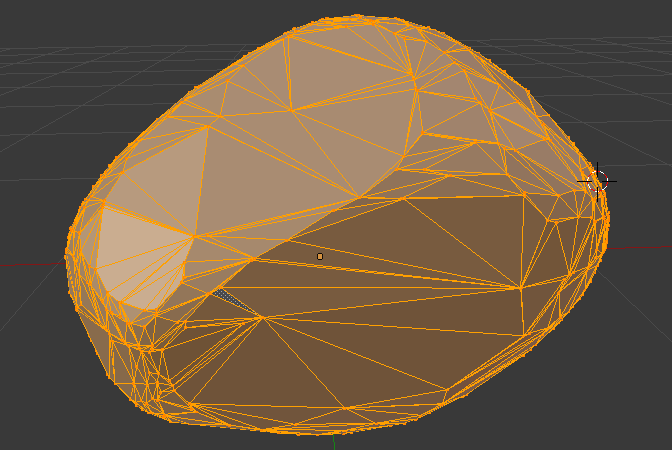
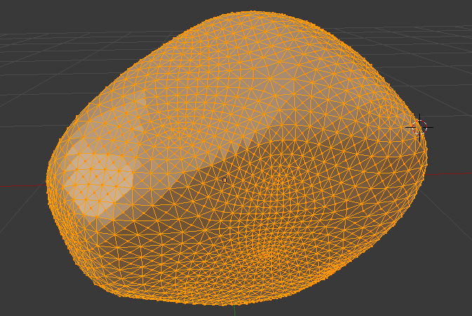
Figure 4: Example shape before (left) and after (right) remeshing operation. See text for detailed description.

4.2 Confidence level of the nominal model

Before cloning of the nominal model can begin a confidence level of the nominal model needs to be established. Later, based on it, the decision whether to accept or reject a clone is made. For a set of observations, against which the model is tested, weighted root-mean-square deviation is calculated:

$$RMSD_{ref}=\sqrt{\frac{\sum_{i}^{N}w_{i}(O_{i}-C_{i})^{2}}{N\sum w_{i}}}$$ (6)

where $O_{i}$ and $C_{i}$ denote observed and corresponding synthetic photometric points and $N$ denotes total number of them. The weight $w_{i}$ is connected with magnitudes precision of a photometric point $\sigma_{i}$, i.e. $w_{i}=1/\sigma_{i}^{2}$.

Next, a standard error of $RMSD_{ref}$ distribution of a form

$$\mathcal{E}=\frac{RMSD_{ref}}{\sqrt{N-n}}$$ (7)

with model’s $n$ degrees of freedom is used to establish a test for the clones. Accepted ones need to satisfy the following equation:

$$RMSD_{clone}\leqslant RMSD_{ref}+\mathcal{E}.$$ (8)

Altogether, we are interested in the clones with the level of goodness of the fit equal or better than the nominal model, as established by $\mathcal{E}$.

Lightcurve comparison is straightforward. Synthetic lightcurves are created for every corresponding available observation. As the absolute magnitude information is absent, the synthetic lightcurves are shifted so that average magnitudes of real and synthetic observations match in each lightcurve. Then, $RMSD$ value is calculated per lightcurve according to eq. 6.

The absolute sparse photometry is processed differently. The increased brightness of asteroids evident in observations taken near opposition (i.e. phase angle less than $8^{\circ}$) depends on spectral type, is non-linear and strongly depends on on the surface properties (Belskaya & Shevchenko, 2000; Muinonen et al., 2010). In the context of this work non-linear part of a phase curve does not contain any crucial, additional information compared to the linear part of a phase curve. To minimise the risk of bad fitting, and therefore influencing the results, we omit the data with phase angles smaller than $8^{\circ}$.

For the remaining linear part the $Ax+B$ function is fitted to the data (separately for real and synthetic observations). The slope parameter $A$ is calculated simultaneously for all data points, while $B$ is calculated separately for each of group of data points with similar aspect angles, with $5^{\circ}$ resolution of the bins. The $RMSD$ value comes from the discrepancy of $B$ parameters. That way we can search for proper z-scale.

$RMSD_{ref}$ value in eq. 8 is the sum of separately computed values for each observation type.

4.3 Surface fluctuations

Introduction of surface fluctuation to the nominal model is achieved by moving its vertices according to one of precomputed convolution masks. A set of convolution masks created beforehand enables testing of the uniformity of changes applied later to any model and is computationally more efficient than doing it ad hoc. Below we describe how convolution masks are created.

Rather than changing vertex positions independently the hills and concavities of various shapes and sizes are introduced. First, a vector $v_{i}$ is randomly selected and it’s position from the centre is randomly changed within $0.5$ to $1.5$ range of initial distance from body centre. Then, all other vertices are being altered as well in order to ensure smooth surface. If $\alpha_{ij}$ is an angle between the two vertices $v_{i}$ and $v_{j}$, then the formula

$$v^{\prime}_{j}=v_{j}A\sin(\alpha_{max}/2)\exp(-2k\alpha_{ij}/\alpha_{max}),$$ (9)

where $A\in[-0.25,0.7]$, $\alpha_{max}\in[50\degree,90\degree]$ and $k\in\{1,2,3\}$ are random numbers, will generate hills or concavities of different width and flatness when applied to vertex distances from the model’s centre. The amplitude $A\sin(\alpha_{max}/2)$ controls the proportion of the base to the hight of a hill and its range is specifically chosen to eliminate undesired spikes or deep wells in resulting body.

Changes to a vertex positions in set of convolution masks are generated randomly but should have uniform distribution not to introduce biases in clones. Because vertices are not independent of each other, special care has to be taken to achieve that. In the set of convolution masks certain amplitude of change for given vertex must appear fixed number of times. With this criterion, when analysing the probability of a vertex having certain amplitude of change the same distribution for each vertex is accomplished. The variances of probability density distributions for vertices’ changes differ by only $0.1\%$ – a satisfactory level of homogeneity.

4.4 Procedure

The algorithm of volume uncertainty assessment described here is based upon the idea of changing the nominal model’s parameters and testing modified models, i.e. clones, against observations. There are three components considered when modifying the nominal model: the spin axis orientation, the scale along the spin axis and surface fluctuations. Combining the scanning of pole position and $z$-axis scale for each surface fluctuation mask in straight forward manner would be computationally heavy so a special strategy needs to be applied in order to assess uncertainty in reasonable time, namely, the procedure consists of two phases.

In the first stage the nominal model is modified only by applying the z-scale drawn from $[0.5,1.5]$ range and by changing the spin axis orientation within $\pm 30^{\circ}$ in both $\lambda$ and $\beta$. For all of the observations synthetic ones are created and compared. The criterion used here differs slightly from eq.8, i.e.

$$RMSD_{clone}\leqslant RMSD_{ref}+3\mathcal{E}.$$ (10)

The surface fluctuations do not alter the volume, lightcurve amplitude and absolute photometry as much as changing spin axis and z-scale do. This fact is used to preselect the space of $\lambda$, $\beta$ and z-scale for the second stage therefore significantly lowering the amount of computation. Altogether, this stage generates a list of $\lambda$, $\beta$, z-scale triples that passed the criterion.

In the second stage all components are joined together. To produce a clone one of the surface fluctuation convolution masks is applied to the nominal model. Subsequently, a triple is randomly drawn from the list created in the previous stage so that the model can be scaled by z-scale and assigned new spin axis orientation. In total there are $1.3\times 10^{6}$ clones created and each of them is tested against eq. 8 thus producing a final population of accepted clones.

To assess volume and parameters’ uncertainties the population of accepted clones is analysed and extrema are searched for. Reported uncertainties are simply a range of values in this population for each parameter. Because of the fact that the hills and concavities have different influence on the lightcurves the uncertainties above and below nominal value are reported separately.

5 Uncertainty propagation

5.1 Volume

Asteroid shape models from lightcurve inversion are dimensionless. The vertex positions are expressed in the units of the longest vector length $R_{max}$, and the volume in $R_{max}^{3}$. By convenience $R_{max}$ is set to 1. The volume uncertainty for unscaled model – which comes from extreme values of accepted clones – is given as percentage of nominal model’s volume.

Even though the models are unitless the information about the volume can be extracted by scaling the clones to match the amount of reflected light by the nominal model which is directly connected to the surface area. Let us consider 3-axial ellipsoid and one photometric point taken at opposition when axis $a$ is pointing towards, and $b$ and $c$ axes perpendicular to, the observer. When all three axes are enlarged uniformly in a clone and when it is uniformly scaled so that the luminosities match we get the same body size and volume. The shape of the lightcurve from larger clone is exactly the same and there is no reason to consider this clone to be different from the nominal model. In contrast, if axis $a$ alone is enlarged, the amount of light stays the same if one uses geometric scattering law, or changes slightly with more sophisticated one. Therefore, there is no imperative to scale the whole model (or is to scale it only a little bit), and so its volume is larger when compared to the reference model. The opposite would happen if we fix axis $a$ and enlarge axes $b$ and $c$.

This simple example gets very complicated quickly if we consider lightcurves covering partial or full rotation rather then single points, additional observations from different positions and phase angles, various spin axis orientations, etc. We can learn about the volume range from clones statistics (an average of all the effects), i.e. the scope of solutions allowed by photometric observations.

5.2 Scale

Scaling methods (e.g. fit to stellar occultation chords, thermophysical modelling, adaptive optics images) provide the scale $S$ by which every vertex of the model can be multiplied to create a model with dimensions expressed in physical units. Scale, in that sense, can be understood as $R_{max}$.

The volume of a scaled model can be expressed as

$$V_{m}=V^{\prime}S^{3}\pm u(V_{m}),$$ (11)

where $V^{\prime}$ is a dimensionless volume of unscaled model and $u(V_{m})$ is volume uncertainty.

When scaling the model using different data type from the one used when creating the model, and such is the case for majority of lightcurve based models, the resultant scale is biased by the model itself. This bias can, and should, be included in the uncertainty of the scale (and scaled volume as well) by accounting for both measurement and model uncertainties during the scaling procedure.

When fitting to the occultation cords or adaptive optics images the positions of the edges of the model on the Earth’s surface or plane-of-sky projections can be transformed from deterministic values into stochastic ones utilizing population of accepted clones created during uncertainty assessment procedure.

In case of observations in thermal infrared, which are not so sensitive to the details of the shape (Hanuš et al., 2015), one could use the information about allowed range of the z-scale as well as spin axis orientation uncertainty when creating thermophysical models. Granted that observations in thermal infrared provide absolute fluxes they are sensible to the extent of the body along the spin axis. Changes in z-scale and spin axis will be apparent in flux – aspect angle relation and could provide better fits to the data when they deviate from a nominal shape model.

5.3 Rotational period and phase of rotation

Rotational period is not a free parameter of a clone. The rotational phase for reference epoch uncertainty $u(\gamma_{0})$ (i.e. uncertainty of the rotational phase at $JD_{0}$) depends on rotational period uncertainty, data points precision and density of the lightcurves and observations’ time span. For each clone the period $P$ and $\gamma_{0}$ are calculated separately from the best fit to synthetic lightcurves. Discrepancy of the values in the accepted clones population for both are treated as their uncertainties. The nature of $\gamma_{0}$ uncertainty is different from the rotational phase uncertainty mainly because it does not accumulate with time. These values have to be added together in order to facilitate total rotational phase uncertainty.

The uncertainty of rotational period propagates into phase of rotation. The rotational phase uncertainty should stay on the same level inside the interval between the first and the last observation because the period was established using all the available lightcurves at once. Outside this time interval rotational phase uncertainty increases linearly with time from the last observation. To facilitate the above in one formula we put the reference epoch right in the middle of observing time span, i.e. $JD_{0}=(JD_{last}+JD_{first})/2$, and then calculate

$$u(\gamma) =\frac{2\pi}{P^{2}}\left[a+b+max(-a+b,0)\right]+u(\gamma_{0}),$$ (12)

$$a =|u(P)\Delta t|,$$

$$b =\frac{1}{2}u(P)\Delta T_{obs}$$

where $P$ is a rotational period, $\gamma$ is a rotational phase, $\gamma_{0}$ is a rotational phase for reference epoch $JD_{0}$, $\Delta T_{obs}=JD_{last}-JD_{first}$ is an observations’ time span, $\Delta t=t-JD_{0}$ is a distance in time from the reference epoch, and $u(x)$ denotes uncertainty of $x$. The $max$ function returns larger of the two arguments. An example plot of this function is shown in Fig. 5.

Figure 5: The plot of total rotation phase uncertainty. In this example $\Delta T_{obs}=38.5$ years, the uncertainty of rotation phase for reference epoch $JD_{0}$ is $u(\gamma_{0})=3^{\circ}$ and the period uncertainty $u(P)=1.5\times 10^{-6}~{}h$ .

6 synthetic example

In order to test the method and show how the dataset influences the model uncertainty we created 3 sets of synthetic lightcurves of a 3-axial ellipsoid with $a/b=1.5$ and $b/c=1.14$. These lightcurves served as reference observations. The body used for testing was the same ellipsoid but with two craters put at ($40^{\circ}$, $0^{\circ}$) and ($305^{\circ}$, $-40^{\circ}$) longitude and latitude coordinates. We wanted to test whether the craters – treated as fictitious features of the body – will be detected as the surface areas with large uncertainty. Moreover, gaps in the rotational phase were introduced in one of the sets and were expected to influence the uncertainty as well. In summary, modified ellipsoid with craters was being altered during the process and compared with lightcurves of an ellipsoid.

6.1 Lightcurves

3 datasets were created, A, B and C. Each consist of $8$ apparitions evenly distributed on the orbit (Fig. 8). The target’s and the observer’s orbits were circular with semi-major axes $a_{\text{target}}=3$ and $a_{\text{obs}}=1$; apparitions were one year apart. The rotational period of the body was $P=4.12345$h and pole orientation was $\lambda=0^{\circ}$, $\beta=45^{\circ}$. For such pole latitude the whole body is visible for the observer if the target’s and observer’s orbits are coplanar and the apparitions are evenly distributed. Had $\beta$ been $\pm 90^{\circ}$ all the lightcurves would have looked the same and more than one lightcurve would have helped only for rotational period estimation, whereas $\beta=0^{\circ}$ would produce at least two flat lightcurves with no shape information in them. There was no Gaussian noise added to the photometric data points.

Dataset A consisted of 24 lightcurves covering full rotational period. Each apparition had 3 lightcurves with phase angles $18.5^{\circ}$ pre opposition, $0^{\circ}$ and $18.5^{\circ}$ post opposition. Dataset B was reduced to 8 lightcurves (one per apparition) with $18.5^{\circ}$ pre opposition phase angle. Comparison of lightcurves from dataset A with the greatest RMSD is shown in Fig. 6.

Dataset C was based on dataset B, but the coverage of the rotational phase was limited, namely, lightcurves covered $3/8$ of the rotational period. One of the lightcurves is presented in Fig. 7. In the body’s reference frame the observer was situated along longitudes from $270^{\circ}$ to $45^{\circ}$. The choice of longitudes’ range was motivated by the positions of the craters which were desired to be covered in the lightcurves.

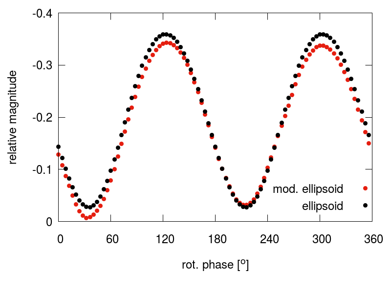
Figure 6: Comparison of synthetic lightcurves of 3-axial ellipsoid and ellipsoid with two craters with the largest RMSD value of $0.0155$. Lightcurves were obtained at $18.5^{\circ}$ phase angle at $6^{th}$ apparition. (see Fig. 8)

Figure 7: Comparison of synthetic lightcurve of 3-axial ellipsoid and ellipsoid with two craters with limited viewing geometries taken at $18.5^{\circ}$ phase angle at $8^{th}$ apparition with $\lambda_{obs}=315^{\circ}$ (see Fig. 8).

Figure 8: The image shows the distribution of apparitions (with the observer in the centre of the graph) in heliocentric reference frame. See text for detailed description.

6.2 Results and discussion

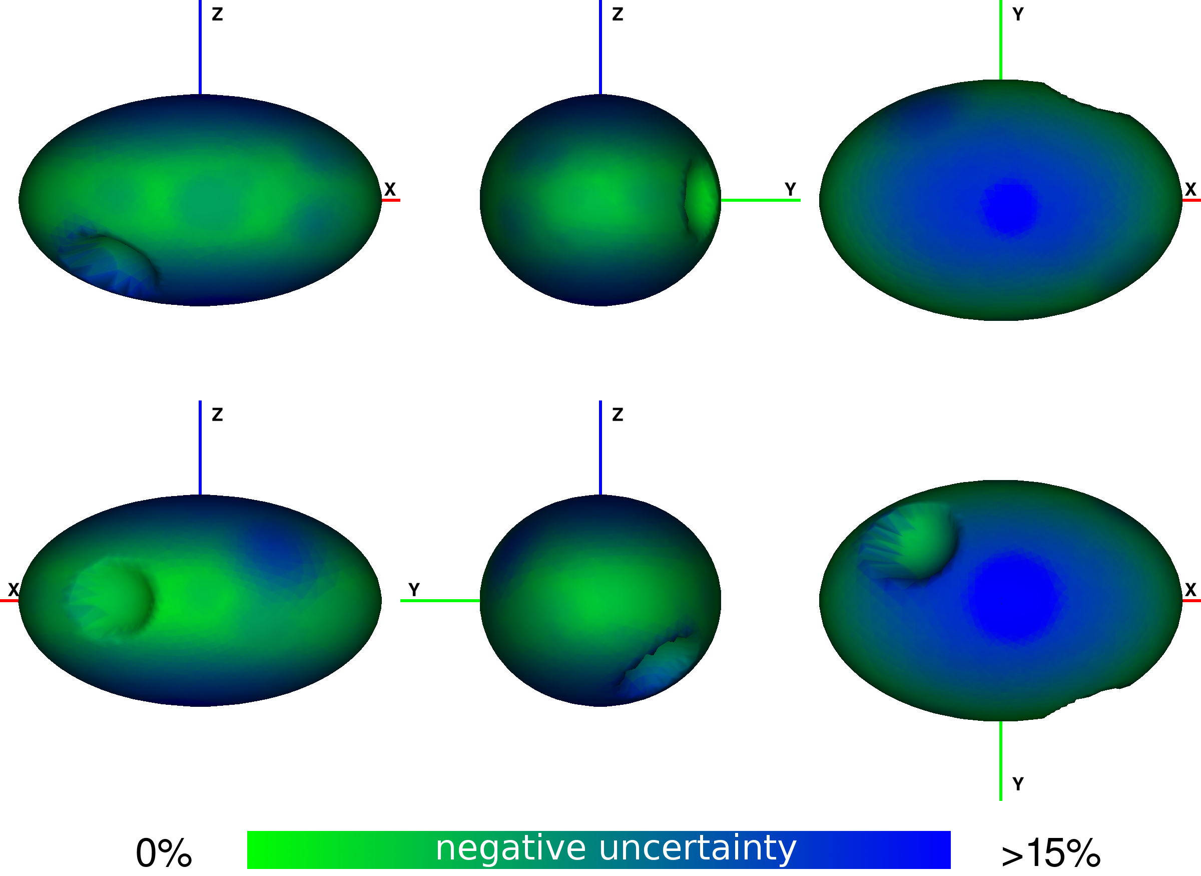
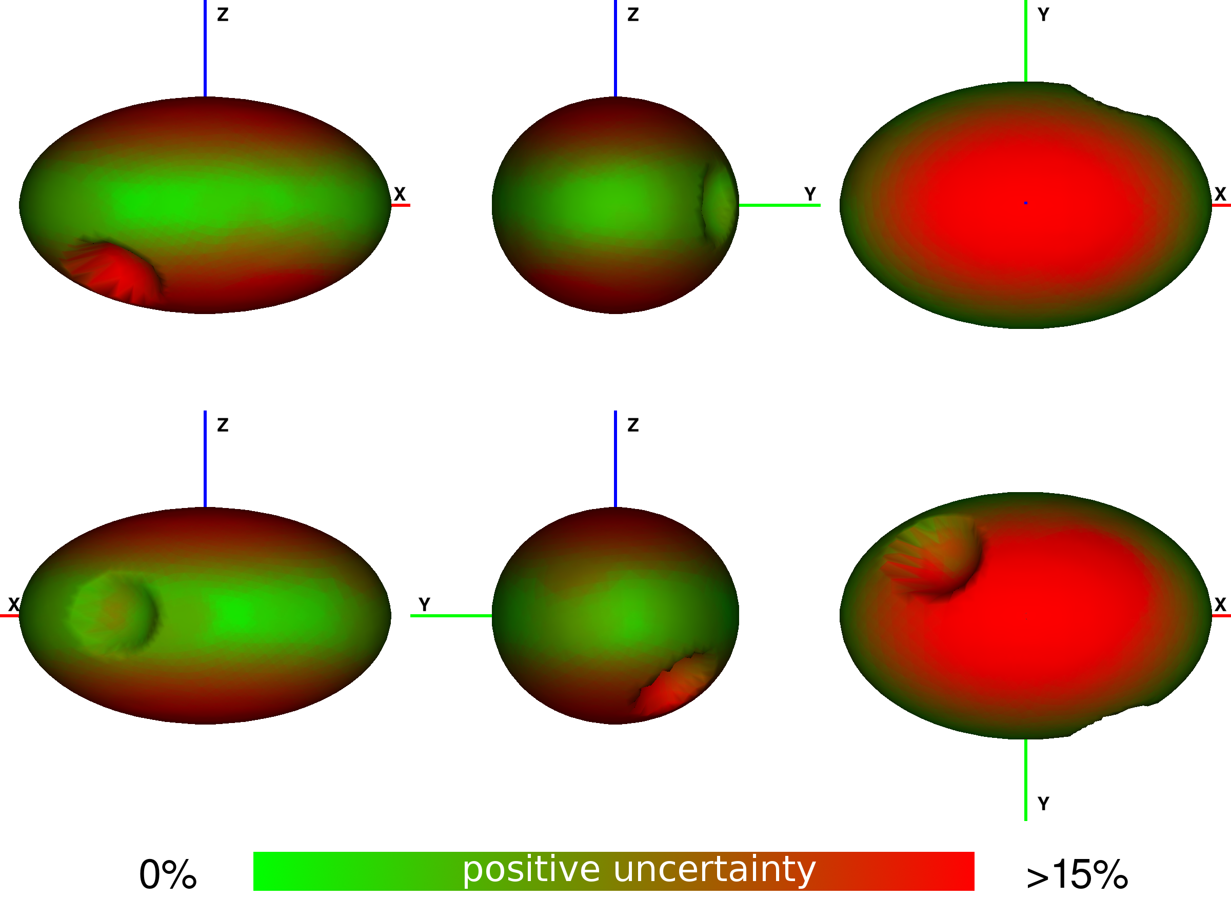
Figure 9: Projections of the target with colour-coded uncertainty information in regard to dataset C. The uncertainty values come from the range of values found in accepted clones population. Top figure shows uncertainty due to changes that create concavities (blue colour) while the bottom shows the hills (red). The scale of the values is the same for the two uncertainty maps, the brightest blue/red showing the values $>=10\%$ of $R_{max}$.

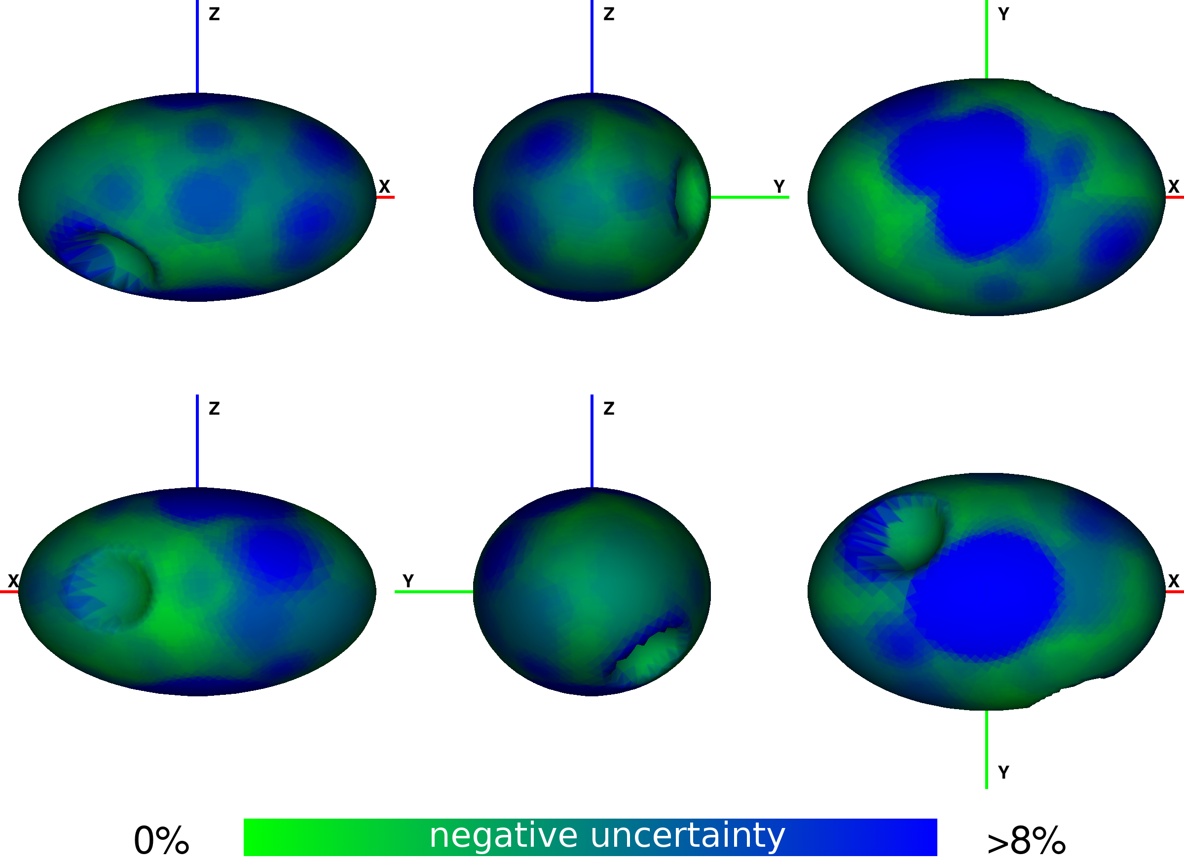
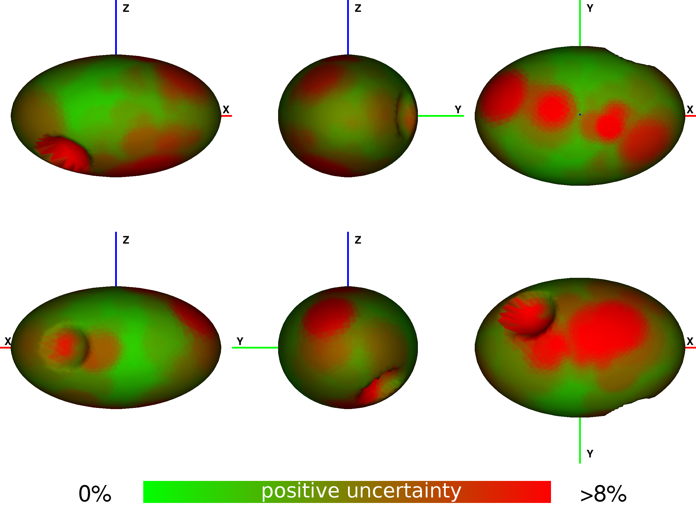
Figure 10: Projections of the target with colour-coded uncertainty information in regard to dataset C and with subtracted z-scale value, thus showing only surface fluctuations part of uncertainties. See text and Fig. 9 for detailed description.

To compute uncertainty of the volume we searched for the largest and the smallest body among the accepted clones. Parameters’ uncertainties were acquired similarly, i.e. by searching for the minimal and maximal values of given parameter in the population as was the case for the rotational period uncertainty as well. For dataset A there were $77162$ clones out of $1.3\times 10^{6}$ that satisfied Eq. 8, while for datasets B and C there were $65474$ and $21435$ of them. The results are summarised in Tab. 1.

The reason why the number of accepted clones decreased as datasets B and C were depleted is that the bigger range of spin axis positions were allowed due to larger standard error $\epsilon$ of nominal model’s initial fit. During initial scan and using Eq. 10 the range of spin axis orientation and z-scales is preselected is wider as $\epsilon$ gets bigger. Because the number of clones in kept constant, after introducing surface fluctuations more clones were subsequently rejected by the criterion given by Eq. 8. The bigger the $\epsilon$ is, the worse – or more quantized – statistics we get. The number of accepted clones is however still big enough, that parameters’ and volume’s uncertainties are not affected much when minimal and maximal values from accepted clones population are used to determine uncertainties. However, the chances to miss an important outlier increase.

In all examples the biggest uncertainties of shape parameters were correlated with the z-scale. As shown in Fig. 9 the areas near the poles dominate at the level of $18\%$ for positive, and $21\%$ for negative values. In all datasets the surface fluctuations induced volume changes smaller than changing the spin axis orientation and z-scale did. The difference in volume between the unmodified ellipsoid and the one with craters was $2\%$. Lightcurves from dataset C yielded, unsurprisingly, the biggest total volume uncertainty of $52\%$. Full lightcurves in dataset B resulted in lower volume uncertainty of $20\%$, whereas the richest dataset A resulted in $12\%$.

Further analysis indicates that the uncertainty in the examples can be divided into two categories: the small effect connected with surface fluctuations and the large effect connected with the z-scale alone. Shown in Fig. 10 are projections of the test body neglecting the z-scale. To achieve that, parameters were referenced not to the nominal body, but to the body already scaled in z-axis before surface fluctuations were added. For negative part, largest values were still situated near the poles and dropped to $18\%$ for negative part. The viewing geometries allowed those areas to be pushed inside without affecting visible cross-section and thus the lightcurves. As for the positive uncertainties, the maximal values of $15\%$ were situated at the positions of the craters. The surface inside the craters was allowed to move outwards without changing the lightcurves meaningfully until it reached the level of the unmodified ellipsoid surface. Going further changed the silhouette of the body influencing the lightcurves more dramatically and leading to larger and unacceptable RMSD values. The uncertainties measured as percentage of $R_{max}$ along the ray originating in the body’scentre correspond to the craters’ depth measured that way.

The geometric scattering law can be treated as a first approximation of any more sophisticated one. The area of the body’s projection on the observer’s field of view has by far the biggest influence on the amount of reflected light. That means, that elements perpendicular to the observer change the amount of light the most if moved (especially outwards). Even though observer saw only $135^{\circ}$ of the rotation phase almost the whole body was represented in the lightcurves in that sense. The parts that were not have much larger uncertainty (up to $8\%$, besides the craters). The gaps in observations allowed invisible parts of the surface to fluctuate more which is apparent along the line from $315^{\circ}$ to $135^{\circ}$ longitudes on the body. The spotted-like nature of uncertainty values, rather than uniform patch, is due to other effects connected with the actual distribution of apparitions on the orbit and the inclination of the pole. Also, the initial discrepancy between the modified and unmodified ellipsoids’ lightcurves (that define the confidence level $\epsilon$) allowed for surface changes away from the craters and unobserved parts.

Table 1: Compilation of results for 3 different datasets. Here we report uncertainties of volume $V$, rotational phase for reference epoch $\gamma_{0}$, rotational period $P$ and spin axis coordinates $\lambda$ and $\beta$.

dataset	$u(V)$[%]	$u(\gamma_{0})[^{\circ}]$	$u(P)$[h]	$u(\lambda)[^{\circ}]$	$u(\beta)[^{\circ}]$
A	${}^{+5}_{-7}$	${}^{+1}_{-1}$	$10^{-6}$	${}^{+1}_{-1}$	${}^{+1}_{-2}$
B	${}^{+5}_{-15}$	${}^{+1}_{-1}$	$3\times 10^{-6}$	${}^{+2}_{-1}$	${}^{+1}_{-4}$
C	${}^{+30}_{-22}$	${}^{+2}_{-2}$	$2\times 10^{-6}$	${}^{+3}_{-2}$	${}^{+8}_{-8}$

7 Uncertainty assessment of selected asteroid models

The method was applied to models of (21) Lutetia, (89) Julia, (243) Ida, (433) Eros, and (162173) Ryugu. Except for Julia, which has adaptive optics images available, each target has been visited by a spacecraft mission resulting in either flyby images or full 3D models that allow comparison of the models derived from photometric data together with their uncertainties. For testing we chose available lightcurve-only based models of those targets. The results are summarised in Tab. 2.

Absolute observations from Oszkiewicz et al. (2011) were used for all of the objects. Their precision was formally at the level of $0.01$ mag. Additionally, for Lutetia, Julia and Ida the Gaia Data Release 2 (Gaia Collaboration et al., 2016, 2018) were also used. The coverage of aspect angles is shown in Fig. 16. We removed data with phase angles less than $8^{\circ}$ (see Sec. 4.2). This resulted in removing 20%, 8%, 38%, 2% and 9% of the data points for Lutetia, Julia, Ida, Eros and Ryugu, respectively. This did not compromise available geometries (i.e. aspect angles) as each apparition had large span of phase angles.

Table 2: Compilation of results for models of (21) Lutetia, (89) Julia, (243) Ida, (433) Eros, and (162173) Ryugu. The uncertainties of volume $V$, rotational phase for reference epoch $\gamma_{0}$, rotational period $P$ and spin axis coordinates $\lambda$ and $\beta$ are reported. The last column describes the best value of z-scale calculated from absolute photometric data.

¹ Torppa et al. (2003); ² this work; ³ Hanuš et al. (2013c); ⁴ Bartczak & Dudziński (2018); ⁵ Müller et al. (2017); model $u(V)$[%] $u(\gamma_{0})[^{\circ}]$ $u(P)$[h] $u(\lambda)[^{\circ}]$ $u(\beta)[^{\circ}]$ z-scale (21) Lutetia¹ ${}^{+9}_{-4}$ ${}^{+4}_{-4}$ $5\times 10^{-6}$ ${}^{+2}_{-1}$ ${}^{+3}_{-3}$ $1.08^{+0.01}_{-0.05}$ (89) Julia² ${}^{+19}_{-15}$ ${}^{+2}_{-2}$ $7\times 10^{-6}$ ${}^{+5}_{-2}$ ${}^{+5}_{-3}$ $0.92^{+0.21}_{-0.06}$ (243) Ida³ ${}^{+51}_{-53}$ ${}^{+12}_{-22}$ $1\times 10^{-5}$ ${}^{+6}_{-4}$ ${}^{+12}_{-22}$ $0.52^{+0.5}_{-0.02}$ (433) Eros⁴ ${}^{+14}_{-20}$ ${}^{+10}_{-4}$ $3\times 10^{-6}$ ${}^{+2}_{-2}$ ${}^{+1}_{-7}$ $1.02^{+0.09}_{-0.09}$ (162173) Ryugu⁵ ${}^{+52}_{-59}$ ${}^{+100}_{-90}$ $1\times 10^{-3}$ ${}^{>+30}_{<-30}$ ${}^{>+30}_{<-30}$ $0.92^{+0.09}_{-0.11}$

7.1 (21) Lutetia

Table 3: Details of the lightcurve data used for (21) Lutetia modelling and uncertainty assessment. N_lc – number of lightcurves per apparition, $\alpha$ – phase angle, $\lambda$ – ecliptic longitude, $\beta$ – ecliptic latitude.

Apparition	Year	Nlc	$\alpha$ $[^{\circ}]$	$\lambda$ $[^{\circ}]$	$\beta$ $[^{\circ}]$	reference
1	1962	30	28	18	-3	Chang & Chang (1963)
2	1981	76	6 – 21	347 – 14	-3	Lupishko et al. (1983) , Zappala et al. (1984)
3	1983	4	3 – 28	130	2	Zappala et al. (1984), Lupishko et al. (1983)
4	1985	75	5 – 24	34 – 46	-2	Dotto et al. (1992), Lupishko et al. (1987)
						Lagerkvist et al. (1995)
5	1986	1	7	60	-1	Lupishko et al. (1987)
6	1991	4	16	173	3	Lagerkvist et al. (1995)
7	1995	12	2	178	3	Denchev et al. (1998)
8	1998	6	26	115 – 120	2	Denchev (2000), private communication
9	2003	20	5 – 29	223 – 229	2	Carry et al. (2010a)
10	2004	7	17	5	-3	Carry et al. (2010a)
11	2005/2006	14	12 – 21	134 – 142	3	Carry et al. (2010a)
12	2007	1	3	212	2	Carry et al. (2010a)
13	2008/2009	23	4 – 25	69 – 95	-1 – 1	Carry et al. (2010a)
14	2010	12	7 – 16	165	2	Carry et al. (2010a)

Asteroid (21) Lutetia has been imaged by Rosetta mission during 10 July 2010 flyby on its way to comet 67P/Churyumov-Gerasimenko. Combining spectrophotoclinometry technique used on flyby images with inversion of photometric lightcurves and adaptive optics images, 3D shape model has been created by Sierks et al. (2011). Only the northern hemisphere was observed during the flyby hence the need for external data to complete unseen half of the body. Later comparison of lightcurve and adaptive optics based model form KOALA method (Carry et al., 2010b; Drummond et al., 2010) with flyby model yielded very good agreement of those models, volume discrepancy (based on equivalent sphere diameters) being better than 10% (Carry et al., 2012).

As our method considers disk-integrated data only we used lightcurve-only based convex model of Lutetia (Torppa et al., 2003). The set of observations is shown in Tab. 3. Upon visual inspection the convex shape model is in very good agreement with the flyby model, especially in $xy$ plane. Nonetheless, convex nature of the model and it being based on lightcurve data prevent the model to represent local topographic features.

The analysis yielded maximum parameters’ uncertainty of $-13\%$ and $10\%$ of $R_{max}$ with well constrained spin axis orientation (uncertainty blow $6^{\circ}$). Convex and flyby model projections comparison is presented in Fig. 11. The biggest values of uncertainties correspond to purely constrained z-scale in lightcurves. Local uncertainties correspond nicely with the parts of the body that shows disagreement with the flyby model. What is more, the parts that do agree (e.g. silhouette in $xy$ plane) are also well constrained by observational data.

Figure 11: (21) Lutetia model (Torppa et al., 2003) projections showing uncertainty values (left and right columns) with comparison to Rosetta mission flyby, lightcurve and adaptive optics based model (centre column) (Sierks et al., 2011).

7.2 (89) Julia

Table 4: Details of the lightcurve data used for (89) Julia modelling and uncertainty assessment. N_lc – number of lightcurves per apparition, $\alpha$ – phase angle, $\lambda$ – ecliptic longitude, $\beta$ – ecliptic latitude.

Apparition	Year	Nlc	$\alpha$ $[^{\circ}]$	$\lambda$ $[^{\circ}]$	$\beta$ $[^{\circ}]$	reference
1	1968	5	5	326 – 329	4	Vesely & Taylor (1985)
2	1972	8	5 – 13	318 – 322	2	Schober & Lustig (1975)
3	2009	18	19 – 24	0 – 6	13	Hanuš et al. (2013b)
4	2017	7	18 – 21	331 – 334	6	Warner (2018)

Although asteroid (89) Julia was not visited by any spacecraft mission it has available set of adaptive optics images (Vernazza et al., 2018) from limited geometries with aspect angles ranging from $123^{\circ}$ to $140^{\circ}$ and revealing mostly southern hemisphere of the body. The non-convex model created for the purpose of this work is based on lightcurve data only (Tab. 4) and was obtained using SAGE method (Bartczak & Dudziński, 2018). Adaptive optics images were used to compare the model and uncertainties. The comparison of the model with uncertainties to VLT/SPHERE images can be seen in Fig. 12.

The non-convex SAGE model did not represent big concavities visible in the images very well. Nonetheless, the model agrees with disk-resolved images within uncertainties (maximal values for parameter were $-20\%$ and $22\%$). The parts where discrepancies are the biggest had the largest uncertainty values, which indicates limited information content in the lightcurves.

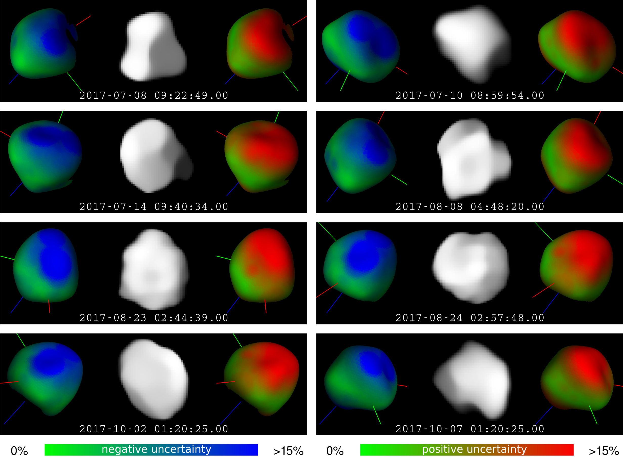
Figure 12: Comparison of (89) Julia obtained with SAGE method (Bartczak & Dudziński, 2018) (left and right) with adaptive optics VLT/SPHERE images (Vernazza et al., 2018) (centre). The model axes $x$, $y$ and $z$ are represented by red, green and blue lines, respectively.

7.3 (243) Ida

Table 5: Details of the lightcurve data used for (243) Ida modelling and uncertainty assessment. N_lc – number of lightcurves per apparition, $\alpha$ – phase angle, $\lambda$ – ecliptic longitude, $\beta$ – ecliptic latitude.

Apparition	Year	Nlc	$\alpha$ $[^{\circ}]$	$\lambda$ $[^{\circ}]$	$\beta$ $[^{\circ}]$	reference
1	1980	9	16	321	0	Binzel et al. (1993)
2	1984	6	3	244	-1	Binzel (1987)
3	1988	15	23 – 15	158 – 180	0	Binzel et al. (1993)
4	1990	130	18	339 – 5	1	Gonano-Beurer et al. (1992), Binzel et al. (1993)
5	1991/1992	67	2 – 30	67 – 93	1	Binzel et al. (1993), Mottola et al. (1994)
6	1992/1993	79	12 – 29	165 – 182	-1	Binzel et al. (1993), Mottola et al. (1994),
						Slivan & Binzel (1996)
7	1993	3	25	76	1	Binzel et al. (1993)

Asteroid (243) Ida was observed by Galileo spacecraft on 28 August 1993. The images obtained during flyby were used to derive 3D shape model (Thomas et al., 1996; Stooke, 2016). Convex, lightcurve based model (see Tab. 5 for description of used observations) of Ida was used (Hanuš et al., 2013c) to assess uncertainties and compare to flyby model.

Upon first look at images in Fig. 13 the convex model is too extent in z-axis, which is reflected in large ranges of parameter uncertainties ($-35\%$ for negative and $50\%$ for positive uncertainties) and in volume uncertainty of more than $100\%$. The model, being convex, does not reproduce concavities, but negative uncertainties are big in the areas where flyby model have them. Regions that do match flyby model well have small uncertainties.

Figure 13: (243) Ida model (Hanuš et al., 2013c) projections showing uncertainty values (left and right columns) with comparison to Galileo mission flyby based model (centre column) (Stooke, 2016).

7.4 (433) Eros

Table 6: Details of the lightcurve data used for (433) Eros modelling and uncuncertainty assessment. N_lc – number of lightcurves per apparition, $\alpha$ – phase angle, $\lambda$ – ecliptic longitude, $\beta$ – ecliptic latitude.

Apparition	Year	Nlc	$\alpha$ $[^{\circ}]$	$\lambda$ $[^{\circ}]$	$\beta$ $[^{\circ}]$	reference
1	1951/1952	28	19 – 59	5 – 119	-10 – 22	Beyer (1953),
2	1972	1	17	342	9	Dunlap (1976)
3	1974/1975	68	9 – 44	53 – 158	-31 – 33	Cristescu (1976), Dunlap (1976),
						Millis et al. (1976),
						Miner & Young (1976), Pop & Chis (1976),
						Scaltriti & Zappala (1976), Tedesco (1976)
4	1981/1982	4	29 – 54	42 – 126	-17 – 37	Drummond et al. (1985), Harris et al. (1999)
5	1993	8	1 – 18	296 – 308	-1 – 4	Krugly & Shevchenko (1999)

(433) Eros is an object from Near Earth Asteroid population that has been extensively studied in the past both remotely and in situ. The NEAR Shoemaker probe, which started orbiting Eros in year 2000 and ended the mission by landing on the surface in 2001, delivered a detailed 3D shape model (Zuber et al., 2000).

The lightcurve-only non-convex model of Eros was modelled with SAGE method and yielded great similarity to the real shape (see Bartczak & Dudziński (2018) for detailed comparison of the shapes, and Fig. 14 for comparison with uncertainties). The lightcurve data was very rich (109 lightcurves) and spanned over long period of 42 years (see Tab. 6).

(433) Eros and (243) Ida are similar cases, both real shapes being alike. Eros, however, has spin axis orientation ($\lambda,\beta=17^{\circ},9^{\circ}$ ) much more favorable in regard to lightcurve inversion compared to Ida’s spin axis ($\lambda,\beta=259^{\circ},-66^{\circ}$). The volume uncertainty for Eros is $36\%$, much smaller in comparison to Ida’s, partially due to more advantageous geometry, and partially due to non-convex nature of the model. Uncertainties show that general features, e.g. crater in the middle (which does not have round edges otherwise preventing it from being represented in the lightcurves) or global curvature of the model in $xy$ plane, are preserved, although the dent in the middle (in $-y$ direction) could be either much deeper or shallower.

Figure 14: (433) Eros model (Bartczak & Dudziński, 2018) projections showing uncertainty values (left and right columns) with comparison to model from NEAR Shoemaker mission (Zuber et al., 2000) (centre column).

7.5 (162173) Ryugu

Table 7: Details of the lightcurve data used for (162173) Ryugu modelling and uncertainty assessment. N_lc – number of lightcurves per apparition, $\alpha$ – phase angle, $\lambda$ – ecliptic longitude, $\beta$ – ecliptic latitude.

Apparition	Year	Nlc	$\alpha$ $[^{\circ}]$	$\lambda$ $[^{\circ}]$	$\beta$ $[^{\circ}]$	reference
1	2007	23	41 – 25	307 – 350	5	Müller et al. (2011, 2017), T. Müller, private communication
2	2007	12	49 – 79	13 – 61	5 – 1
3	2008	11	88 – 54	127 – 186	-5
4	2011	1	55	349	6
5	2011	1	76	62	1
6	2012	34	0 – 49	215 – 277	-3 – 3
7	2013	2	47	57	1
8	2013	2	52	146	-6
9	2016	12	43 – 17	264 – 305	1 – 5

Near Earth Asteroid (162173) Ryugu has been intensely studied since it has been selected as Hayabusa-2 sample return mission target. The shape model used in this work is taken from Müller et al. (2017), where authors studied thermophysical properties of Ryugu. The search for the spin axis and shape proved to be very challenging and both optical and thermal data were used to find the solution, since the lightcurve amplitude is very low (0.2 mag) with small signal-to-noise ratio. See Tab. 7 for the description of lightcurves for this target. The shape was suspected to be nearly spherical with spin axis orientation $\lambda,\beta=340^{\circ},-40^{\circ}$. The Hayabusa-2 images revealed Ryugu’s bi-cone top shape and most probably rubble pile structure, as well as ecliptic latitude of rotational axis orientation $\beta=-87.45\pm 0.03^{\circ}$ (Hirata et al., 2018) (see Fig. 15 for comparison).

The model of Ryugu is far from what in situ observations have unveiled, particularly when it comes to spin axis orientation. The uncertainties of $\lambda$ and $\beta$ justly reached the limits of scanning area, which is $\pm 30^{\circ}$ from the nominal solution. The uncertainty of rotational phase angle was as high as $190^{\circ}$ with $10^{-3}$ rotational period level of precision because of low lightcurve amplitude and, therefore, ability to recognise distinct features in them.

Huge uncertainties in all tested parameters show that the method can serve as a good indicator of model’s robustness. Low quality observational data in case of Ryugu produced large span of acceptable spin orientations (see Tab. 1 and Fig. 1 in Müller et al. (2017)). For the purpose of this work we used SAGE algorithm (Bartczak & Dudziński, 2018) on Ryugu’s data as well. The solution space was vast with plethora of local minima with no shape and spin solution being significantly better than other. Uncertainty assessment definitely revealed the problematic nature of this target.

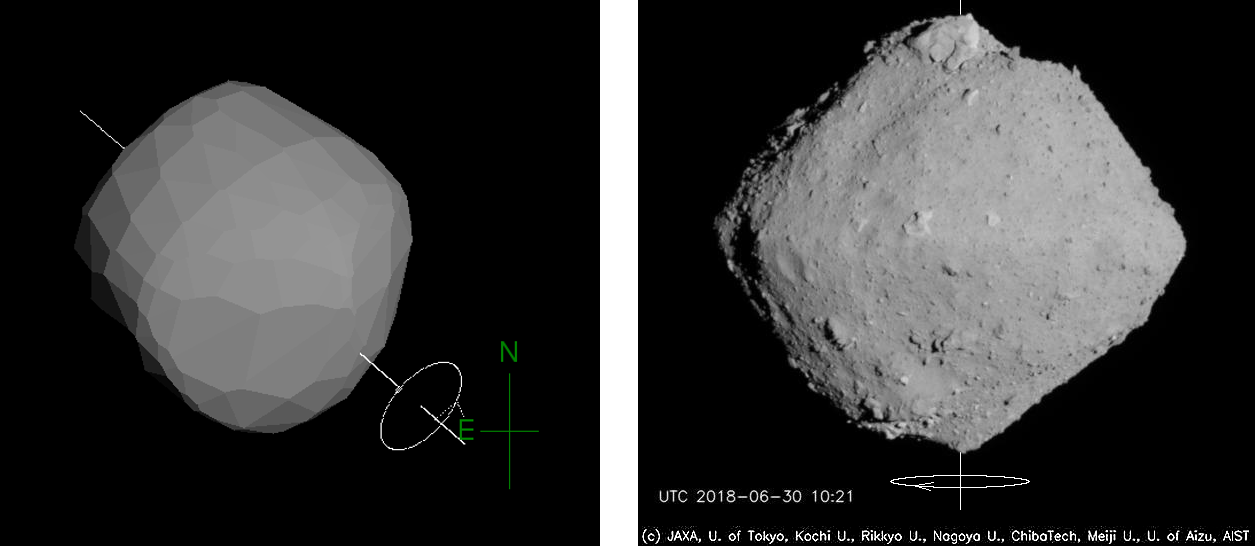
Figure 15: Comparison of asteroid (162173) Ryugu convex model (Müller et al., 2017) (left) with image aquired by Hayabusa-2 mission (source: www.hayabusa2.jaxa.jp) on 30 June 2018 (right).

7.6 z-scale from absolute photometry

From the fact that absolute photometry was used during uncertainty assessment procedure, the information on the best z-scale can be extracted. The results of the search for the best z-scale are presented in the last column of Tab. 2.

A problem not taken into consideration in the estimate presented in Sec. 3.1 is the influence of the phase angle. The nature of the surface of the body has major influence on the slope parameter. Additionally, the position of terminator coupled with the shape defines the fraction of the body being in the shadow and subsequently the phase dependent decrease in magnitudes. Also, due to the rotation of a target and resulting amplitude of reflected light, data points are scattered along the mean value. The sampling is not random and can influence the value of slope parameter as well. The z-scale is burdened with all if the effects combined.

The z-scales found correspond with the differences between lightcurve-based and in situ models, particularly evident in case of (243) Ida. Moreover, the uncertainties of the z-scales correspond with the available ranges of aspect angles. Assuming nominal spin axes orientations, the absolute photometry aspect angles are presented on Fig. 16.

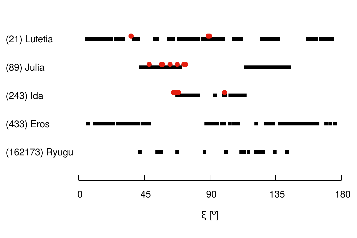
Figure 16: Plot showing absolute photometry aspect angles $\xi$ coverage. Black lines correspond to data from Oszkiewicz et al. (2011) while red dots show Gaia DR2 measurements.

8 Conclusions

We created an uncertainty assessment method which can be applied to asteroid models with reference to lightcurves and absolute sparse data in visual bands. The method is effective as a measure of information content stored in lightcurves – something any lightcurve inversion method is lacking – and has informative role considering asteroid models’ robustness adding new dimension into the evaluation process. It was applied to a small sample of synthetic and real targets showing that it can transform qualitative evaluation (Sec. 2 and 3) into quantitative one.

The results presented in this work indicate that shape and, therefore, other physical parameter (e.g. volume or density) uncertainties of lightcurve-based models are likely to be vastly understated. A large sample of models needs to be examined in order to shed a new light on this matter. By far, the unknown extent of the model along its spin axis has the biggest influence on the volume uncertainty. Establishing proper z-scale depends on the available aspect angles and the photometric precision of the observational dataset. The lightcurve inversion should definitely make use of absolute photometry, especially precise and homogeneous Gaia dataset, during the modelling process to produce more reliable models volume-wise.

Preliminary assessment of volume uncertainty from available geometries, as shown in Sec. 3, requires prior knowledge about the spin axis. For the same reason, specific observing strategies could only be established for, and applied to targets with known parameters in order to improve the existing models. Collecting as much data as possible, evenly distributed on the orbit and with the best achievable quality seems to be the only general recipe one could give to assure low uncertainty of the models. The Minor Planet Bulletin’s continuously updated list of lightcurve photometry opportunities (e.g. Warner et al. (2018)) created for observation optimization concerning asteroid models can be utilised for exactly that purpose.

When equivalent sphere diameters are being reported their uncertainties come solely from the fit of the deterministic model (e.g. an ellipsoid, 3D shape from lightcurve inversion) to the absolute measurements like stellar occultation chords, adaptive optics images or thermal data. The uncertainties of the models themselves are not considered at all. Making asteroid models’ observation predictions for various techniques (e.g. lightcurves, stellar occultations, adaptive optics images, radar delay-Doppler images, thermal emission) is necessary to allow the computation of sizes taking models’ uncertainty into account. In order to achieve that, each data point has to have probability distribution associated with it that has its source in model uncertainty. Stochastic models of asteroids can be attained from the clone population created during the uncertainty assessment procedure presented in this work. Exploiting them will result in more realistic uncertainties of derived quantities.

Studying large sample of models, creating observation predictions and incorporating other observational techniques into the uncertainty assessment process are the areas which should definitely be explored further.

References

- Alí-Lagoa et al. (2018) Alí-Lagoa V., Müller T. G., Usui F., Hasegawa S., 2018, A&A, 612, A85
- Bartczak & Dudziński (2018) Bartczak P., Dudziński G., 2018, MNRAS, 473, 5050
- Barucci & Fulchignoni (1982) Barucci M. A., Fulchignoni M., 1982, Hvar Observatory Bulletin, 6, 157
- Barucci et al. (1982) Barucci M. A., et al., 1982, Moon and Planets, 27, 387
- Belskaya & Shevchenko (2000) Belskaya I. N., Shevchenko V. G., 2000, Icarus, 147, 94
- Berthier et al. (2014) Berthier J., Vachier F., Marchis F., Ďurech J., Carry B., 2014, Icarus, 239, 118
- Beyer (1953) Beyer M., 1953, 281, 121
- Binzel (1987) Binzel R. P., 1987, Icarus, 72, 135
- Binzel et al. (1993) Binzel R. P., et al., 1993, Icarus, 105, 310
- Carry (2012) Carry B., 2012, Planet. Space Sci., 73, 98
- Carry et al. (2008) Carry B., Dumas C., Fulchignoni M., Merline W. J., Berthier J., Hestroffer D., Fusco T., Tamblyn P., 2008, A&A, 478, 235
- Carry et al. (2010a) Carry B., et al., 2010a, Icarus, 205, 460
- Carry et al. (2010b) Carry B., et al., 2010b, A&A, 523, A94
- Carry et al. (2012) Carry B., et al., 2012, Planet. Space Sci., 66, 200
- Catmull & Clark (1978) Catmull E., Clark J., 1978, Computer-Aided Design, 10, 350
- Chang & Chang (1963) Chang Y. C., Chang C. S., 1963, Acta Astron Sinica, 11, 139
- Cristescu (1976) Cristescu C., 1976, Icarus, 28, 39
- D’Ambrosio et al. (1985) D’Ambrosio V., Burchi R., di Paolantonio A., Giuliani C., 1985, Astronomy and Astrophysics, 144, 427
- Denchev et al. (1998) Denchev P., Magnusson P., Donchev Z., 1998, Planet. Space Sci., 46, 673
- Dotto et al. (1992) Dotto E., Barucci M. A., Fulchignoni M., di Martino M., Rotundi A., Burchi R., di Paolantonio A., 1992, A&AS, 95, 195
- Drummond et al. (1985) Drummond J. D., Cocke W. J., Hege E. K., Strittmatter P. A., 1985, Icarus, 61, 132
- Drummond et al. (2010) Drummond J. D., et al., 2010, A&A, 523, A93
- Dunlap (1976) Dunlap J. L., 1976, Icarus, 28, 69
- Ďurech et al. (2011) Ďurech J., et al., 2011, Icarus, 214, 652
- Gaia Collaboration et al. (2016) Gaia Collaboration et al., 2016, A&A, 595, A1
- Gaia Collaboration et al. (2018) Gaia Collaboration et al., 2018, A&A, 616, A1
- Gonano-Beurer et al. (1992) Gonano-Beurer M., di Martino M., Mottola S., Neukum G., 1992, A&A, 254, 393
- Hanuš et al. (2013a) Hanuš J., Marchis F., Ďurech J., 2013a, Icarus, 226, 1045
- Hanuš et al. (2013b) Hanuš J., Marchis F., Ďurech J., 2013b, Icarus, 226, 1045
- Hanuš et al. (2013c) Hanuš J., et al., 2013c, A&A, 559, A134
- Hanuš et al. (2015) Hanuš J., Delbo’ M., Ďurech J., Alí-Lagoa V., 2015, Icarus, 256, 101
- Hanuš et al. (2011) Hanuš J., et al., 2011, A&A, 530, A134
- Harris et al. (1999) Harris A. W., Young J. W., Bowell E., Tholen D. J., 1999, Icarus, 142
- Hirata et al. (2018) Hirata N., et al., 2018, in AAS/Division for Planetary Sciences Meeting Abstracts. p. 501.05
- Kaasalainen & Torppa (2001) Kaasalainen M., Torppa J., 2001, Icarus, 153, 24
- Kaasalainen et al. (2001) Kaasalainen M., Torppa J., Muinonen K., 2001, Icarus, 153, 37
- Kaasalainen et al. (2002a) Kaasalainen M., Mottola S., Fulchignoni M., 2002a, Asteroid Models from Disk-integrated Data. pp 139–150
- Kaasalainen et al. (2002b) Kaasalainen M., Torppa J., Piironen J., 2002b, Icarus, 159, 369
- Kaasalainen et al. (2005) Kaasalainen M., Hestroffer D., Tanga P., 2005, in Turon C., O’Flaherty K. S., Perryman M. A. C., eds, ESA Special Publication Vol. 576, The Three-Dimensional Universe with Gaia. p. 301
- Krugly & Shevchenko (1999) Krugly Y. N., Shevchenko V. G., 1999, in Lunar and Planetary Science Conference.
- Kryszczyńska et al. (2007) Kryszczyńska A., La Spina A., Paolicchi P., Harris A. W., Breiter S., Pravec P., 2007, Icarus, 192, 223
- Lagerkvist et al. (1995) Lagerkvist C.-I., et al., 1995, A&AS, 113, 115
- Lupishko et al. (1983) Lupishko D. F., Belskaya I. N., Tupieva F. A., 1983, Pisma v Astronomicheskii Zhurnal, 9, 691
- Lupishko et al. (1987) Lupishko D. F., Velichko F. P., Bel’Skaia I. N., Shevchenko V. G., 1987, Kinematika i Fizika Nebesnykh Tel, 3, 36
- Magnusson et al. (1989) Magnusson P., Barucci M. A., Drummond J. D., Lumme K., Ostro S. J., Surdej J., Taylor R. C., Zappalà V., 1989, in Binzel R. P., Gehrels T., Matthews M. S., eds, , Asteroids II. pp 66–97
- Marciniak et al. (2015) Marciniak A., et al., 2015, Planet. Space Sci., 118, 256
- Marciniak et al. (2018) Marciniak A., et al., 2018, A&A, 610, A7
- Mignard et al. (2007) Mignard F., et al., 2007, Earth Moon and Planets, 101, 97
- Millis et al. (1976) Millis R. L., Bowell E., Thompson D. T., 1976, Icarus, 28, 53
- Miner & Young (1976) Miner E., Young J., 1976, Icarus, 28, 43
- Mottola et al. (1994) Mottola S., Gonano-Beurer M., Green S. F., McBride N., Brinjes J. C., di Martino M., 1994, Planet. Space Sci., 42, 21
- Muinonen et al. (2010) Muinonen K., Belskaya I. N., Cellino A., Delbò M., Levasseur-Regourd A.-C., Penttilä A., Tedesco E. F., 2010, Icarus, 209, 542
- Müller et al. (2011) Müller T. G., et al., 2011, A&A, 525, A145
- Müller et al. (2017) Müller T. G., et al., 2017, A&A, 599, A103
- Oszkiewicz et al. (2011) Oszkiewicz D. A., Muinonen K., Bowell E., Trilling D., Penttilä A., Pieniluoma T., Wasserman L. H., Enga M.-T., 2011, J. Quant. Spectrosc. Radiative Transfer, 112, 1919
- Pajuelo et al. (2018) Pajuelo M., et al., 2018, Icarus, 309, 134
- Pop & Chis (1976) Pop V., Chis D., 1976, Icarus, 28, 37