$S^{2}$-LBI: Stochastic Split Linearized Bregman Iterations for Parsimonious Deep Learning

Abstract

This paper proposes a novel Stochastic Split Linearized Bregman Iteration ($S^{2}$-LBI) algorithm to efficiently train the deep network. The $S^{2}$-LBI introduces an iterative regularization path with structural sparsity. Our $S^{2}$-LBI combines the computational efficiency of the LBI, and model selection consistency in learning the structural sparsity. The computed solution path intrinsically enables us to enlarge or simplify a network, which theoretically, is benefited from the dynamics property of our $S^{2}$-LBI algorithm. The experimental results validate our $S^{2}$-LBI on MNIST and CIFAR-10 dataset. For example, in MNIST, we can either boost a network with only 1.5K parameters (1 convolutional layer of 5 filters, and 1 FC layer), achieves 98.40% recognition accuracy; or we simplify $82.5\%$ of parameters in LeNet-5 network, and still achieves the 98.47% recognition accuracy. In addition, we also have the learning results on ImageNet, which will be added in the next version of our report.

1 Introduction

The expressive power of Deep Convolutional Neural Networks (DNNs) comes from the millions of parameters, which are optimized by various algorithms such as Stochastic Gradient Descent (SGD) Bottou (2010), and Adam Kingma and Ba (2015). Remarkably, the most popular deep architectures are manually designed by human experts in some common tasks, e.g., object categorization on ImageNet. In contrast, we have to make a trade-off between the representation capability and computational cost of networks in the real world applications, e.g., robotics, self-driving cars, and augmented reality. On the other hand, some experimental results show that classical DNNs may be too complicated for most specific tasks, e.g., “reducing $2\times$ connections without losing accuracy and without retraining” in Han et al. (2015b).

To explore a parsimonious deep learning structure, recent research focuses on employing Network Architecture Search (NAS) Elsken et al. (2018) and network pruning Han et al. (2015a). Practically, the computational cost of NAS algorithms themselves are prohibitive expensive, e.g., 800 GPUs concurrently at any time training the algorithms in Zoph and Le (2016). Furthermore, network pruning algorithms Han et al. (2015a); Abbasi-Asl and Yu (2017); Molchanov et al. (2017) introduce additional computational cost in fine-tuning/updating the networks. In addition, some works study the manually designed compact and lightweight small DNNs, (e.g. ShuffleNet Ma et al. (2018), MobileNet Howard et al. (2017), and SqueezeNet Iandola et al. (2017)), which, nevertheless, may still be tailored only for some specific tasks.

The additional computational cost of NAS and pruning algorithm, is due to the fact that the SGD algorithms and its variants, e.g., Adam, do not favor a parsimonious training with increasing levels of structural sparsity (e.g. (group) sparsity in fully connected/convolutional layer). More specifically, the SGD algorithms, in principle, do not have an intrinsic feature selection mechanism in deep network (Sec. 2.3). One has to associate the loss function with some sparsity-enforcement penalties (e.g. Lasso), and for each of the regularization parameters typically in a decreasing sequence, SGD runs to seek a convergent model which is nearly never met in deep learning and then pursue various sparse models. In such a homotopy computation of Lasso-type regularization paths, various models along the SGD path have never been fully explored in any previous works.

In this paper, we propose a natural algorithm that can simultaneously follow a path of SGD training of deep learning while pursuing model structures along the path. The algorithm lifts the original network parameters, say $\Theta$, to a coupled parameter set, say $(\Theta,\Gamma)$. While a usual stochastic gradient descent runs over the primal parameter $\Theta$, a sparse proximal gradient descent (or mirror descent, linearized Bregman iterations) runs over the dual parameter $\Gamma$ which enforces structural sparsity on network models. These two dynamics are coupled using a proximal gap penalty in loss function. Then the algorithm returns an iterative path of models with multiple levels of structural sparsity. During the training process, the earlier a network structure parameters becomes non-zero, the more important is the model structure. Similarly, the larger is the magnitude of $\Gamma$, the more influence on prediction it has. Such a feature can be used to construct various network structures parsimoniously with as good a prediction performance as possible. This algorithm is inspired by a recent development of differential inclusion approach to boosting with structural sparsity that improves the Lasso path in model selection Huang et al. (2016a, 2018) and has been successfully used in machine vision Zhao et al. (2018) and neuroimage analysis Sun et al. (2017). In this paper we adopt such an idea for the development of a novel network training algorithm, called Stochastic Split Linearized Bregman Iteration ($S^{2}$-LBI) algorithm.

By virtue of solution path, we further propose the forward/backward selection algorithms by $S^{2}$-LBI to learn to add/remove parameters of networks. As a result, network structures can be “shaped” via forward or backward regularization solution path computed by $S^{2}$-LBI. For the forward direction, the forward selection algorithm can dynamically expand from an initial small network into a reasonable large one, as shown in Fig. 1 for illustration. In more details, at each stage, $S^{2}$-LBI can be trained to gradually fit data. Equipped with an early stopping scheme, the model can avoid overfitting in the current parameter space. Then we lift the parameter space into a higher dimensional space by adding more randomly initialized parameters (e.g. filters or neurons) and continue training again. In contrast, by configuring the solution path in a backward manner, the backward selection algorithm can simplify or prune the initial large network to a small reasonable one. Specifically, the $S^{2}$-LBI can efficiently learn the importance of the parameters by measuring their selection order and magnitudes. By ranking the importance of parameters into a descending order and remove the low rank parameters, the network can thus be shrunken without losing much representation (thus prediction) power.

Figure 1: Illustration of forward algorithm. Blue represents accuracy curve, while red vertical line denotes the point at which we add new parameters. During training, the accuracy curve tends to increase with new parameters dynamically added, which lift the parameters into a higher dimensional space. When new parameters added, the accuracy decreases a little since the new random initialized parameters, and increases with fine-tuning.

Contributions. (1) We, for the first time, propose a novel $S^{2}$-LBI algorithm that can efficiently compute the regularization solution path of deep networks. $S^{2}$-LBI algorithm can efficiently train a network with structural sparsity. (2) In the forward manner, our forward selection algorithm can dynamically and incrementally expand from a small initial network into a large network one. (3) In the backward manner of solution path, our backward selection algorithm can simplify the network without deteriorating the prediction performance. Extensive experiments on two datasets, validate the efficacy of our proposed algorithms.

2 Stochastic Linearized Bregman Iteration

In a supervised learning task, we denote $f_{\Theta}:\mathbf{\mathcal{X}}\to\mathbf{\mathcal{Y}}$ as the mapping function of neural network architecture with $L$ layers, with weight parameters $\Theta=\{W^{1},...,W^{L}\}$, from input space $\mathbf{\mathcal{X}}$ and output space $\mathbf{\mathcal{Y}}$. The $W^{l}$ is the weight matrix between $l$-th layer and ($l$+1)-th layer, i.e. $\mathcal{O}^{l+1}=\sigma(W^{l}\mathcal{O}^{l})$ where $\mathcal{O}^{l}$ denotes the output of the $l$-th layer and $\sigma$ is the activation function (e.g. relu,sigmoid). Denote $\Theta_{-W^{l}}$ as $\{W^{1},...,W^{l-1},W^{l+1},...,W^{L}\}$. Given training data $\mathbf{X}\overset{\Delta}{=}\{\mathbf{x}_{1},...,\mathbf{x}_{N}\}$ and $\mathbf{Y}\overset{\Delta}{=}\{\mathbf{y}_{1},...,\mathbf{y}_{N}\}$, we denote $\mathcal{L}(f_{\Theta}(\mathbf{X}),\mathbf{Y})$ as the loss function. For classification task with $\mathbf{\mathcal{Y}}=[K]\overset{\Delta}{=}\{1,...,K\}$, the $\mathcal{L}$ can be written as:

$$\mathcal{L}(f_{\Theta}(\mathbf{X}),\mathbf{Y})=\frac{1}{N}\sum_{i=1}^{N}\sum_{k\in[K]}\mathbf{1}(\mathbf{y}_{i}=k)\log{\frac{1}{p(f_{\Theta}(\mathbf{x}_{i})=k)}},$$

We use $\mathcal{L}(\Theta)$ to denote the loss function for simplicity. Generally, the mini-batch SGD algorithm update $\Theta$ as follows:

$$\Theta_{t+1}=\Theta_{t}-\alpha\cdot\nabla_{\Theta}L\left(\Theta_{t}\right)|_{(\mathbf{X},\mathbf{Y})_{{\mathrm{batch_{t}}}}}$$ (1)

where $\Theta_{t}\overset{\Delta}{=}\{W_{t}^{l}\}_{l\in[L]}$ is the parameter value at the $t$-th step, $\alpha$ is the learning rate, $(\mathbf{X},\mathbf{Y})_{{\mathrm{batch_{t}}}}$ represents the batch-sample at the $t$-th iteration. For simplicity, we omit $(\mathbf{X},\mathbf{Y})_{{\mathrm{batch_{t}}}}$ in the rest of the paper.

2.1 Sparsity enforcement via $\ell_{1}$ regularization

To achieve sparsity on a weight matrix at the $l$-th layer ($W^{l}$), one can apply $\ell_{1}$-based regularization $\Omega(W^{l})$, which turns the loss function as

$$\mathcal{L}_{\lambda}(\Theta)=\mathcal{L}(\Theta)+\lambda\cdot\Omega\left(W^{l}\right)$$ (2)

where $\lambda$ is the regularization hyper-parameter. The choice of $\Omega(\cdot)$ is determined by the form of $W^{l}$:

• When $W^{l}$ denotes filters at the $l$th layer, $\Omega(\cdot)$ is the group-lasso penalty Yuan and Lin (2006), which aims at group-wise sparsity. Specifically, $W^{l}$ can be re-denoted as $W_{\mathrm{conv}}\overset{\Delta}{=}\left[w_{\mathrm{conv}}^{1,\top},...,w_{\mathrm{conv}}^{G,\top}\right]^{\top}$ with $G$ filters. Then $\Omega(W^{l})\overset{\Delta}{=}\Omega(W_{\mathrm{conv}})=\sum_{g=1}^{G}\|w_{\mathrm{conv}}^{g}\|_{2}$, where $\|w_{\mathrm{conv}}^{g}\|_{2}=\sqrt{\sum_{k}\left(w_{\mathrm{conv}}^{g,k}\right)}$.

• When $W^{l}$ denotes the multiplication matrix before the $l+1$-th fully connected layer, $\Omega(\cdot)$ is lasso-type penalty. The $W^{l}$ is re-denoted as $W_{\mathrm{fc}}$, and $\Omega(W^{l})\overset{\Delta}{=}\Omega(W_{\mathrm{fc}})=\sum_{i,j}|W_{\mathrm{fc}}(i,j)|$.

This common $\ell_{1}$ regularization strategy can be adopted to prune the network, such as Liu et al. (2017); Wen et al. (2016b). However, note that the regularization hyper-parameter $\lambda$, which determines the sparsity level of parameters, is the trade-off between under-fitting and over-fitting. Hence, one should choose an appropriate $\lambda$, which is often typically achieved via prediction error on cross-validation. In more details, one has to run SGD several times over a grid of $\lambda$’s, which brings out a large computational cost, especially for deep neural network. In the next section, we will introduce an iterative algorithm which can return a regularization solution path, which is called Stochastic Split Linearized Bregman Iteration ($S^{2}$-LBI).

2.2 $S^{2}$-LBI algorithm

Here we present the Stochastic Split Linearized Bregman Iteration algorithm, which we will see later, can efficiently learns the regularization solution path in optimizing neural networks. Rather than directly dealing with the sparsity of $W^{l}$, we exploit an augmented variable $\Gamma^{l}$ and want it to (i) be enforced with sparsity (ii) be kept close to $W^{l}$ via variable splitting term $\frac{1}{2\nu}\|W^{l}-\Gamma^{l}\|_{2}^{2}$ with hyper-parameter $\nu>0$. Combined with such a variable splitting term, the loss function of $S^{2}$-LBI turns to

$$\bar{\mathcal{L}}\left(\Theta,\Gamma^{l}\right)=L\left(\Theta\right)+\frac{1}{2\nu}\left\|\Gamma^{l}-W^{l}\right\|_{2}^{2}$$ (3)

Now consider the following iterative algorithm for t=1,…,T:

$$\Theta_{-W^{l},t+1} =\Theta_{-W^{l},t}-\alpha\cdot\nabla_{\Theta_{-W^{l}}}\bar{\mathcal{L}}\left(\Theta,\Gamma^{l}\right)$$ (4a)

$$W^{l}_{t+1} =W^{l}_{t}-\kappa\cdot\alpha\cdot\nabla_{W^{l}}\bar{\mathcal{L}}\left(\Theta,\Gamma^{l}\right)$$ (4b)

$$Z^{l}_{t+1} =Z^{l}_{t}-\alpha\cdot\nabla_{\Gamma}\bar{\mathcal{L}}\left(\Theta,\Gamma^{l}\right)$$ (4c)

$$\Gamma^{l}_{t+1} =\kappa\cdot\mathrm{Prox}_{\Omega}\left(Z^{l}_{t+1}\right)$$ (4d)

$$\widetilde{W}^{l}_{t+1} =\mathrm{Proj}_{\mathrm{supp}(\Gamma^{l}_{t+1})}(W^{l}_{t+1})$$ (4e)

With $Z^{l}_{0}=\Gamma^{l}_{0}=0$, $\Theta_{0}$ can be randomly initialized from Gaussian Distribution, and hyper-parameters $\nu,\kappa,\alpha>0$. The $Z$ here is an auxiliary parameter used for gradient descent w.r.t. $\Gamma^{l}$, where by Moreau decomposition $Z=\Gamma+\partial(\Omega(\Gamma))/\kappa$. The sparsity of $\Gamma$ is achieved by proximal map in (4d) associated with $\Omega\left(\cdot\right)$, of which the general form is

$$\mathrm{Prox}_{\Omega}\left(Z\right)=\arg\min_{\Gamma}\frac{1}{2}\|\Gamma-Z\|_{2}^{2}+\Omega\left(\Gamma\right).$$ (5)

At each step, the sparse estimator $\widetilde{W}^{l}_{t}$ is the projection of $W^{l}_{t}$ onto the subspace of support set of $\Gamma^{l}_{t}$, i.e., Eq. (4e) in which

$$\mathrm{Proj}_{\mathrm{supp}(\Gamma)}\left(W^{l}(i,j)\right)=\begin{cases}W^{l}(i,j),\ \ \mathrm{if}\ \Gamma^{l}(i,j)\neq 0\\ 0,\ \ \ \mathrm{otherwise}\end{cases}$$ (6)

Starting from a null model with $\Gamma^{l}_{0}=\widetilde{W}^{l}_{0}=0$, the $S^{2}$-LBI evolves into models $\{\Theta_{t},W^{l}_{t},\Gamma^{l}_{t},\widetilde{W}^{l}_{t}\}$ with different sparsity levels, until the full model in which all parameters in $\Gamma^{l}$ are non-zeros, often-over-fitted. To avoid over-fitting, the early stopping regularization is often required.

Under linear model ($\mathcal{L}$ is the squared loss function) implemented with gradient descent, Eq. (4) degenerates to Split LBI Huang et al. (2016b) with $W$ representing a vector parameter, which is proposed to achieve the structural sparsity ($DW$ is sparse). It was proved that under linear model, the Split LBI can achieve model selection consistency, i.e. (i) the features selected at earlier steps belong to the true signal set $\mathcal{S}=\mathrm{supp}(DW^{\star})$, where $W^{\star}$ is the true signal (ii) successfully recover $\mathcal{S}$ at some iteration. Further, with $D=I$ and $\nu\to 0$, it degenerates to Linearized Bregman Iteration (LBI), which is firstly proposed for image restoration with Total Variation penalty Osher et al. (2005). Although $D=I$ in our scenario, we also adopted the variable splitting term with $\nu>0$, since it was proved that such a term can improve the model selection consistency, especially with larger $\nu$ Huang et al. (2016b). The $S^{2}$-LBI can be regarded as the generalization of Split LBI, in terms of (1) general loss function (2) matrix parameters (3) mini-batch stochastic gradient descent.

At a first glance at loss function $\bar{\mathcal{L}}$ in Eq. (3) and iterative scheme (4), one may ask following two questions: (1) The loss function seems not including regularization function, then how $S^{2}$-LBI achieves sparsity? (2) What’s the loss function of Eq. (4) is optimizing?

In fact, different from the common iterative algorithm in which the estimator in the final step tries to converge to the minimizer of a certain loss function, the $S^{2}$-LBI is the discretization of the following differential inclusion with $\alpha\to 0$,

$$\dot{\Theta}_{-W^{l},t} =-\nabla_{\Theta_{-W^{l}}}\bar{\mathcal{L}}\left(\Theta_{t},\Gamma^{l}_{t}\right)$$ (7a)

$$\frac{\dot{W}^{l}_{t}}{\kappa} =-\nabla_{W^{l}}\bar{\mathcal{L}}\left(\Theta_{t},\Gamma^{l}_{t}\right)$$ (7b)

$$\dot{\Gamma}^{l}_{t}+\frac{\dot{\rho}^{l}_{t}}{\kappa} =-\nabla_{\Gamma}\bar{\mathcal{L}}\left(W_{t},\Theta_{-W_{t}},\Gamma_{t}\right)$$ (7c)

$$\rho^{l}_{t} \in\partial\|\Gamma^{l}_{t}\|_{1}$$ (7d)

where $\rho^{l}_{t}$, as the subgradient of $\ell_{1}$ penalty, together with $\Theta_{t},\Gamma^{l}_{t}$, are right continuously differentiable, $\dot{\rho}^{l}_{t},\dot{\Theta}_{t},\dot{\Gamma}^{l}_{t}$ denote right derivatives in $t$ of $\rho^{l}_{t},\Theta_{t},\Gamma_{t}$, and $\rho^{l}_{0}=0,\Gamma^{l}_{0}=0$, $\Theta_{0}$ is randomly initialized from Gaussian Distribution. We called such a differential inclusion as Stochastic Split Linearlized Bregman Inverse Scale Space ($S^{2}$-LBISS) Osher et al. (2016). The $t$ is regularization hyper-parameter, which determines the sparsity level and hence plays the similar role as $\frac{1}{\lambda}$ in Eq. (2). Compared with $\ell_{1}$ penalty which has to run optimization problem several times, a single run of LBI generates the whole regularization path, hence can largely save the computational cost. Here we give some implementation details of $S^{2}$-LBI (Eq (4)).

• The $\kappa$ is the damping factor, which enjoys the low bias with larger value, however, at the sacrifice of high computational cost. The $\alpha$ is the step size. In Huang et al. (2016b), it has been proved that the $\alpha$ is the inverse scale with $\kappa$ and should be small enough to ensure the statistical property. In our scenario, we set it to 0.01/$\kappa$.

• The $\nu>0$ controls difference between $\widetilde{W}^{l}$ and $W^{l}$, and it is the trade-off between model selection consistency and parameter estimator error. One one hand, as discussed earlier, larger $\nu$ can improve statistical property; on the other hand, too large value of $\nu$ can worsen the estimation of parameters. In our experiments, $\nu$ is often set with appropriately large value, which is also adopted in Sun et al. (2017); Zhao et al. (2018). Particularly, Zhao et al. (2018) discussed that features can be orthogonally decomposed into strong signals (mainly interpretable to the model), weak signals (with smaller magnitude compared with strong ones) and null features. It was proved that when $\nu$ is appropriately large, as the dense estimator $W$ can enjoy better prediction power by leveraging weak signals.

• The $\Gamma$ at each step can be explicitly given by simplifying Eq. (5),

  • $\Gamma^{g}=\kappa\cdot\max(0,1-1/\|Z^{g}\|_{2})Z^{g}$ for $g\in\{1,...,G\}$, when $W$ denotes the filter parameters, i.e. $W_{\mathrm{conv}}$.

  • $\Gamma_{i,j}=\kappa\cdot\max(0,1-1/\|Z(i,j)\|_{2})Z(i,j)$ for $i\in\{1,...,p_{1}\}$ and $j\in\{1,...,p_{2}\}$ when $W\in\mathbb{R}^{p_{1}\times p_{2}}$ denotes the multiplication matrix before the fully connected layer, i.e. $W_{\mathrm{fc}}$.

2.3 From Boosting with Sparsity to $S^{2}$-LBI

The $S^{2}$-LBI can be understood as a form of boosting as gradient descent with structural sparsity via differential inclusion Huang et al. (2018). Particularly, the gradient descent step in (4b) and (4c) can be regarded as a boosting procedure with general loss Mason et al. (1999). For example, $L_{2}$-Boost Bühlmann and Yu (2003) with square loss function can be firstly traced back to Landweber Iteration in inverse problems Yuan et al. (2007). To pursue sparsity, one can adopt FS_ϵ-boosting which updates parameters as follows:

$$W^{d^{\star}}_{k+1}=W^{d^{\star}}_{k}-\epsilon\cdot\mathrm{sign}(g^{d^{\star}}_{k})$$ (8)

where $g_{k}$ is the gradient of $\bar{\mathcal{L}\left(\cdot\right)}$ w.r.t. $W_{k}$ and $d^{\star}:=\arg\max_{(i,j)}|g^{i,j}_{k}|$, and $\epsilon\in(0,1)$ is a small step size to avoid overfitting. The update Eq (8) can be characterized as a steepest coordinate descent, w.r.t., $\ell_{1}$- norm: $\Delta=\arg\max\left\{\langle v,g_{k}\rangle\mid\|v\|_{1}:=\sum_{i,j}\left|A_{i,j}\right|\right\}$.

Mirror Descent. We can achieve sparsity from a more general perspective, i.e. mirror descent algorithm (MDA) Krichene et al. (2015), which is also called proximal gradient descent by extending the Euclidean projection to proximal map associated with a sparsity-enforced Bregman Distance. In our scenario, we consider dynamics

$$\dot{\Theta}_{t} =-\nabla_{\Theta}\bar{\mathcal{L}}\left(W_{t},\Theta_{-W_{t}},\Gamma_{t}\right)$$ (9a)

$$\dot{Z}_{t} =-\nabla_{\Gamma}\bar{\mathcal{L}}\left(W_{t},\Theta_{-W_{t}},\Gamma_{t}\right)$$ (9b)

$$\mathcal{B}^{t} =\partial\Psi^{\star}(\mathcal{U}^{t})$$ (9c)

where $\mathcal{B}\overset{\Delta}{=}[\Theta^{\top},\Gamma^{\top}]^{\top}$, $\mathcal{U}\overset{\Delta}{=}[\Theta^{\top},\Gamma^{\top}]^{\top}$. The $\Phi(\cdot)$ is a general regularization function that is often convex, and $\Phi^{\star}(z)=\max_{x}\langle x,z\rangle-\Phi(x)$. To pursue sparsity, we take $\Psi(\mathcal{B})=\|\Gamma\|_{1}+\frac{1}{2\kappa}\left(\|W^{l}\|_{2}^{2}+\|\Gamma\|_{2}^{2}\right)+\frac{1}{2}\|\Theta_{-W^{l}}\|_{2}^{2}$, then Eq (9) turns to $S^{2}$-LBISS (Eq. (7)).

Similarly, we can also write the discretized form of Eq. (9). It was proved in Krichene et al. (2015) that with smooth $\Psi$ and as $t\to\infty$, we have

$$D_{\Phi}(\mathcal{B}_{t},\mathcal{B}^{\star})=\Psi(\mathcal{B}_{t})-\Psi(\mathcal{B}^{\star})-\langle\partial\Phi(\mathcal{B}^{\star}),\mathcal{B}_{t}-\mathcal{B}^{\star}\rangle$$

where $\mathcal{B}^{\star}\overset{\Delta}{=}\arg\min_{\Theta,\Gamma}\bar{\mathcal{L}}(\Theta,\Gamma)$, which is however not satisfying the statistical property (e.g. model selection consistency) in the sparsity problem, since it is often over-fitted. Hence, to achieve sparsity, rather than the final step of $S^{2}$-LBI, we are more interested in the regularization solution path and the early stopping scheme that can avoid over-fitting.

3 Forward/Backward Selection by $S^{2}$-LBI

In this section, we apply $S^{2}$-LBI on expanding and pruning a neural network. The centered idea of these two tasks is by replacing SGD with $S^{2}$-LBI to train the network.

3.1 Forward Selection: Expanding a Network

Since $S^{2}$-LBI evolves from null model to full model, and tend to select more parameters for $\Gamma$ as the algorithm iterates, we can apply it to expand a network. We take $W_{conv}$ in a certain layer (say, $l$-th layer) as an example for the illustration of how to expand a network using $S^{2}$-LBI. Starting from a small number of filters (e.g. 2) in convolutional layer of network, more and more filters tend to be with non-zero value as the algorithm iterates. At each step, we can compute the ratio of $\widetilde{W}^{g}$ to be non-zero. If this ratio passes a pre-set threshold, we add more convolutional filters (which are randomly initialized) into $W_{k}$, and continue learning the network from training data. More specifically, suppose at iteration $k$, the $l$-th layer has $G_{k}$ filters. With pre-defined selection criterion $s^{l}_{k}:=\#\{g\in[G_{k}]:\|\widetilde{W}_{conv,k}^{g}\|_{2}>0\}/G_{k}$, we determine whether $m$ new filters are added: If the selection criterion $s^{l}_{k}$ exceeds a certain threshold $T$, then $m$ filters will be added, i.e., the number of filters turn to $G_{k}+m$. The newly added parameters are randomly initialized, while the other parameters are kept the same. We call this process as Forward Selection by $S^{2}$-LBI.

Note that the regularization parameter $t$ in Eq. (7) (or $t_{k}=k\cdot\alpha$ in $S^{2}$-LBI) is the trade-off between under-fitting and over-fitting. Therefore, unlike the optimization algorithm in which the estimator of the last step is the optimal one, the $S^{2}$-LBI can be understood as returning a whole regularization solution path from under-fitting to over-fitting, in which the estimators with earlier steps are often under-fitted, and then find the optimal point at some step, until finally over-fitted in the current parameter space as iterates. Hence, to avoid saturating to a local optimal in the current parameter space, we stop training when the algorithm meets the selection criterion, and lift to a higher parameter space by adding new parameters, in order to find “better” optimal point.

3.2 Backward Selection: Pruning a Network

On the other hand, the regularization solution path $\{W_{k},\widetilde{W}_{k},\Gamma_{k}\}$ computed by $S^{2}$-LBI can also be utilized to post-simplify a network when the training process is completed. Specifically, we propose an Order Strategy and Magnitude Strategy by setting some filters/features in $\widetilde{W}_{k}$ to 0. In more details, the Order Strategy records the order that each filter/parameter in $\left\{\widetilde{W}\right\}$ is selected along the solution path. We use $\mathbf{E}$ to record the first epoch that a filter/feature to be non-zeros. The less number of $E$, the more importance of the filter/parameter. Besides, when the training process is completed, we can also compute the $L_{2}$ magnitude $\mathbf{M}$ of each filter/parameter. The larger the value, the more importance of the filter/feature. We then measure the importance of filter/parameter as follows,

$$Sc=\lambda_{1}\cdot\mathbf{M}-\lambda_{2}\cdot\mathbf{E}$$ (10)

where $\lambda_{1},\lambda_{2}>0$. The descending order of $Sc$ ranks the importance of filters/parameters in the network. We can directly set the filters/paramters in $W$ with low rank in $Sc$ as 0. In that follows, we give some explanation of why we use $\mathbf{E}$ and $\mathbf{M}$ to measure the importance.

Explanation of $\mathbf{E}$. As mentioned earlier, the regularization solution path $\{\widetilde{W}_{k},\Gamma_{k}\}$ is proved Huang et al. (2016a) in Genearlized Linear Model (GLM) to enjoy the model selection consistency that the features selected before some point, belong to the true signal set. That means, the Order Strategy is reasonable to measure the importance of the selected features. Specifically, the filter selected at smaller $k$ may be more correlated with $y$. After $k$ passes a threshold, the filters selected are mostly fit random noise, which should hence be removed.

Explanation of $\mathbf{M}$. Zhao et al. Zhao et al. (2018) orthogonally decomposed all features into strong signal, weak signal and null features. The “strong” signals refer to the features selected via sparsity regularization, which corresponds to $\widetilde{W}$ and accounts for the main component of the model hence often have larger magnitudes than rest of the features. The weak signals correspond to the elements with smaller magnitude than strong signals, but larger magnitude than null features. By ranking the ranking the magnitude of learned parameters except for strong signals, the weak signals can be detected unbiasedly as long as $\nu$ is large enough. Moreover, it can be proved theoretically and experimentally that equipped with such weak signals, the dense estimator ($W$) outperforms sparse estimator ($\widetilde{W}$) in the prediction. Thus, the Magnitude Strategy can be leveraged to differentiate weak signals from random noise.

4 Related works

Network Regularization. It is essential to regularize the networks, such as dropout Srivastava et al. (2014) preventing the co-adaptation, and adding $L_{2}$ or $L_{1}$ regularization to weights. In particular, $L_{1}$ regularization enforces the sparsity on the weights and results in a compact, memory-efficient network with slightly sacrificing the prediction performance Collins and Kohli (2014). Further, group sparsity regularization Yuan and Lin (2006) can also been applied to deep networks with desirable properties. Alvarez et al. Alvarez and Salzmann (2016) utilized a group sparsity regularizer to automatically decide the optimal number of neuron groups. The structured sparsity Wen et al. (2016a); Yoon and Hwang (2017) has also been investigated to exert good data locality and group sparsity. In contrast, the regularization term of $S^{2}$-LBI proposed can not only enforce the structured sparsity, but also can efficiently compute the regularization solution paths of each variable.

Expanding a Network. Most previous works of expanding network are mostly focused on transfer learning/ life-long learning Wang et al. (2017); Thrun and Mitchell (1995); Pentina and Lampert (2015); Li and Hoiem (2016), or knowledge distill Hinton et al. (2014). In contrast, to the best of knowledge, this work, for the first time, can enlarge a network in a more general setting in the training process: our strategy is more general and can start from a very small network. The inverse process of growing network, is to simplify a network. Comparing to network pruning algorithms Zhu et al. (2017); Zhou et al. (2017); Jaderberg et al. (2014); Zhang et al. (2016); Han et al. (2015b); Li et al. (2017); Abbasi-Asl and Yu (2017); Yang et al. (2018), our strategy directly removes less important parameters by using the solution path computed by $S^{2}$-LBI. The backward selection algorithm does not introduce any additional computational cost in learning to prune the networks.

regularization solution path. Regularization path is a powerful statistic tool to analysis data and statistic model, it can be used for feature selection. Usually, in linear model, we could set different regularization parameter, and get the regularization path by fitting the model for several times. In contrast, $S^{2}$-LBI is a novel algorithm that could generate regularization solution path in one training procedure. Our $S^{2}$-LBI does not only provide an efficient way of training deep neural network, but also give an intrinsic mechanism of analyzing deep network. Thus built upon $S^{2}$-LBI, we can expand a network. In GLM, our $S^{2}$-LBI will be degenerated into Split LBI Huang et al. (2016a), which satisfies path consistency property that features belong to the true signal set will be firstly selected.

5 Experiments

We conduct experiments to validate $S^{2}$-LBI on MNIST and CIFAR-10. MNIST is a widely used dataset with 60,000 gray-scale handwritten digits of 10 classes. CIFAR-10 is a well-known object recognition dataset, which contains of 60,000 RGB images with size $32\times 32$. It have 10 class with 6000 images per class. We use the standard supervised training and testing splits on both datasets. 20% of training data are saved as the validation set. The classification accuracy is reported on test set of each dataset. Source codes/models would be download-able.

5.1 Expanding a Network

Generally, increasing the number of neurons in the FC layer have much less importance than adding the filters of convolutional layer. For example, Han et al. Han et al. (2015b) can directly prune the fully connected layer, from dense into sparse, without sacrificing the performance. Thus our experiments are designed to show that our $S^{2}$-LBI can successfully and efficiently increase the number of convolutional filers in both dataset. The resulting network can have comparable performance with much less parameters.

	MNIST	CIFAR-10
	Acc.	Acc.(1L)	Acc. (2L)
$S^{2}$-LBI (whole path)	98.30	63.56	74.59
SGD	98.17	65.30	74.51
Adam	98.16	64.73	75.75
$S^{2}$-LBI (forward selection)	98.40	63.44	74.23

Table 1: The results of using different training algorithms to learn the expanded structure of $S^{2}$-LBI. “1L”/ “2L” indicate 1 / 2 convolutional layers.

5.1.1 Expansion on MNIST

We expand a simple CNN network, which only contains one convolutional and one fully connected layer. The initial network structure is defined as conv.c1 ($1@5\times 5$) – Maxpooling($2\times 2$) – FC (144 neurons) – 10 classes, where $1@5\times 5$ means 1 filters with size $5\times 5$, the default activation function – ReLU and and the softmax in classification layer. In our experiments, we set the threshold $T=80\%$. That means, if more than $80\%$ convolutional filters in $W_{conv}^{k}$ are selected into $\widetilde{W}_{conv}^{k}$, our $S^{2}$-LBI will automatically add 2 more convolutional filters into this layer. The weighting connection of Fully Connected (FC) layer will also be correspondingly adapted in connecting to the newly added filters. The newly added parameters are initialized as He et al. (2015).

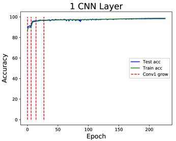
Figure 2: Results of expanding a network on MNIST dataset. The X-axis and Y-axis indicates the training epochs, and classification accuracy on the testing data. The red dash lines indicate 2 new filters are automatically added in that epoch by our $S^{2}$-LBI algorithm. Note that the training process can be early stopping at around 50 epochs; and we show the results of much more epochs to better understand the performance of our $S^{2}$-LBI.

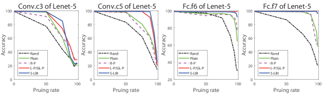
Figure 3: We simplify the LeNet-5 structure on (a) conv.c3 layer, (b) conv.c5 layer, (c) fc.c6 layer, (d) fc.f7 layer. Several different competitors are compared. $S^{2}$-LBI algorithm is employed to train the network.

We show the results of expanding the network in Fig. 2. We can observe that, with only 7 filters (175 parameters) and 1 FC layer (1440 parameters), the expanded network can achieve the classification accuracy of $98.40\%$. The total parameters are 1.6K parameters. In contrast, the LeNet-5 LeCun et al. (1998) is pre-defined network structure which is composed of 3 convolutional layers and 2 fully connected layers. The classification accuracy of LeNet-5 is $\sim 99.0\%$LeCun et al. (1998) with the parameters of 61.5K parameters. We use SGD, rather than $S^{2}$-LBI algorithm to train the same boosting network; and the results are $98.55\%$. This implies that our enlarged network can achieve comparable results as LeNet-5 with much less parameters. More importantly, most of parameters of our enlarged network is automatically added according to the training data without human interaction.

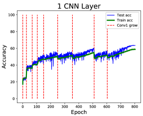
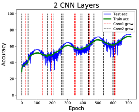
Figure 4: Booting a network in CIFAR-10 dataset.

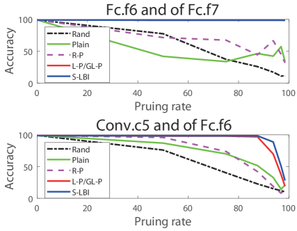
Figure 5: Simplifying two layers in LeNet-5 on MNIST dataset. Each column indicates the percentage of parameter saved on these two layers. Com-Rat, is short for the compression ratio of the total network, i.e., the ratio of saved parameters divided the total number of parameters of LeNet-5.

5.1.2 Expanding a Network in CIFAR-10

We enlarge the CNN network in CIFAR-10 dataset. We adopt two initial networks, (1) Network-1: conv.c1 ($1@5\times 5$) – Maxpooling($2\times 2$) – FC (144 neurons) – 10 classes; (2) Network-2: conv.c1 ($1@5\times 5$) – Maxpooling ($2\times 2$) –conv.c1 ($1@3\times 3$) – Maxpooling($2\times 2$) – FC (36 neurons) – 10 classes. We have default activation function ReLU, and the softmax is used in classification layer. We have the threshold $T=80\%$; and if the ratio of filters selected into $\widetilde{W}_{conv}^{k}$ is higher than the threshold, 2 more filters are automatically added by $S^{2}$-LBI. The connections will be automatically added between FC layers. Only the newly added parameters, which are initialized as He et al. (2015); and we donot re-initialize the parameters of the other parts.

The results are shown in Fig. 4. The final classification accuracy of Network-1 and Network-2 is $63.44\%$ and $74.23\%$ individually. In Network-1, our Forward Selection algorithm results 17 convolutional filters; and Network-2 has 21 and 29 convolutional filters. These results are comparable to those of state-of-the-arts of 1 or 2 layer networks, e.g., 3-Way Factored Restricted Boltzmann Machine (RBM) (3 layers)Ranzato and Hinton (2010) : 65.3%; (2) Mean-covariance RBM (3 layers) Ranzato et al. (2010): 71.0%; (3) SGD: 65.30/74.51, and (4) Adam : 64.73/75.75.

To further compare these results, the resulting networks by forward selection algorithm, are trained by different other optimization algorithms, e.g., SGD, Adam, and $S^{2}$-LBI (whole path). Note that, $S^{2}$-LBI indicates that we directly use the $S^{2}$-LBI to train the fixed networks, rather than employing the Forward Selection algorithm to gradually add filters. All algorithms are trained until it gets converged. The results are summarized in Tab. 1. It shows that the results of our forward selection algorithm are comparable to $S^{2}$-LBI (whole path). Note that both $S^{2}$-LBI (whole path) and $S^{2}$-LBI (forward selection) gets the converged at the same number of training epochs; but the forward selection algorithm has much less computational cost, since the filters are gradually added. Admittedly, the results of SGD, and Adam have slightly better results than those of $S^{2}$-LBI. This is also reasonable. Our $S^{2}$-LBI enforces the structure sparsity to the network, and it can be taken as a set of feature selection algorithms. This is the main advantage over the SGD, and Adam. The other weak features learned in SGD and Adam, (but not selected by $S^{2}$-LBI ) may also be useful in the prediction Zhao et al. (2018). For example, Lasso does not necessarily have better prediction ability than Ridge Regression. To sum up, the results shows that our $S^{2}$-LBI algorithm can efficiently grow a network.

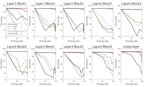
Figure 6: We simplify the ResNet-20 structure trained on CIFAR-10 dataset. Several different competitors are compared. Please refer to supplementary for large figure.

5.2 Simplifying networks

5.2.1 Simplifying networks on MNIST

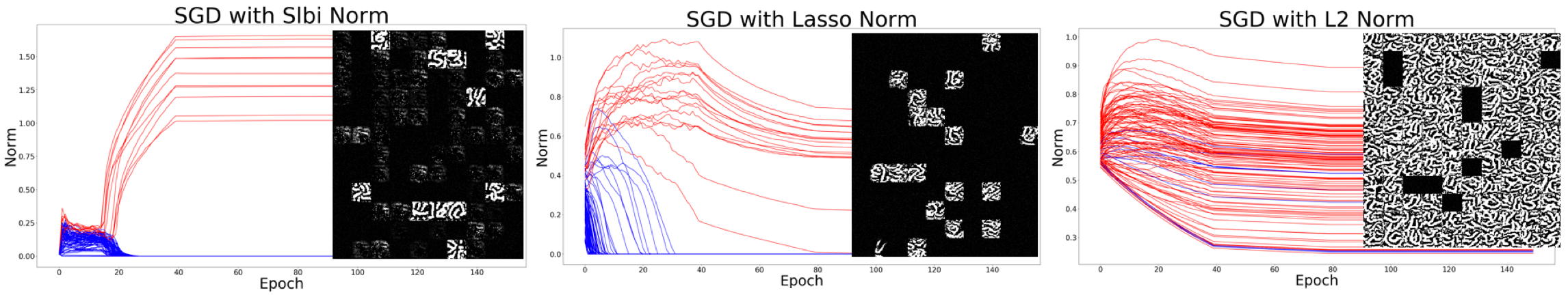
Figure 7: Visualization of solution path and filter patterns. X-axis and Y-axis are the training epochs, and filter magnitude respectively.

Competitors. We compare several other methods of simplifying the networks. (1) Plain: we train a LeNet-5 network; we use $L_{2}-$norm on all parameters with the normalizing coefficient $5e-4$. We rank the importance of weights/filters in term of their $L_{2}$ magnitude values in the descending order and remove those with low rank. This is a naive baseline of our simplifying network algorithm. (2) Rand. We randomly remove the weights or filters in the networks. This is another naive baseline. (3) Ridge-Penalty (R-P) Han et al. (2015b): we use $L_{2}-$norm to penalize one layer of network. Different from Plain, the normalizing coefficient is set as $1e-3$, which is cross validated by searching from $1e-1$ to $1e-5$ on Lenet-5. (4) Lasso-type penalty or Group-Lasso-type penalty (L-P / GL-P): the L-P is used to prune the weights of fully connected layers, and we employ the GL-P to directly remove the filters of convolutional layers. We also cross validate the normalizing coefficient, which is finally taken as $1e-4$. Note that all the results are trained for one time, and we do not have fine-tuning step after the network simplification.

Simplifying one layer. The results are shown in Fig. 3. We use our $S^{2}$-LBI algorithm to train the LeNet-5, and simplify each individual layer of LeNet-5, while we keep the parameters of the other layers unchanged. Note that, the simplified network is not fine-tuned by the training data again. As compared in the Fig. 3, we have the following observations: (1) On two fully connected layers (fc.f6 and fc.f7), both the L-P /GL-P and our simplifying network algorithm work very well. For example, on the fc.f7 layer, our s only has 1.57% of the parameters on these layers. Surprisingly, our performance is only 0.03% lower than that of the original network. In contrast, we compare such results with the baselines: Plain, Rand, and R-P. There is significant performance dropping with the more parameters removed. This shows the efficacy of our algorithm. (2) On the convolutional layer (conv.c5), our results still also achieve remarkable results. The conv.c5 layer has $48k$ out of $61k$ number of parameters of Lenet-5. We show that ours saves 12.5% of total parameters of this layer (i.e., $42k$ number of parameters can be removed on this layer) and the results get only dropped by 0.3%. This demonstrates that our $S^{2}$-LBI indeed can select important weights and filters from $\left\{W^{k}\right\}$ into $\left\{\widetilde{W}^{k}\right\}$ in the $k$-th training epoch. (3) The conv.c3 layer is another convolutional layer in LeNet-5. We found that this layer is very important to maintain a good performance of overall network. Nevertheless, our results are still better than the other competitors.

Simplifying more layers. With the trained model by our $S^{2}$-LBI, we can consider simplifying two layers together, i.e., fc.f6 + fc.f7, or conv.c5+fc.f6 layers, since conv.c5 and fc.f6 have $48k$ and $10k$ number of parameters out of the total $61k$ parameters in LeNet-5. The results are reported in Fig. 5. We can show that our framework can still efficiently compress the network while preserve significant performance. Furthermore, when we simplify the conv.c5 and fc.f6 layers, our model can achieve the best and efficient performance. With only 17.60% parameter size of original LeNet-5, our model achieves the performance as high as 98.47%. Remarkably, our simplifying algorithm does not need any fine-tuning and re-training steps. This shows the efficacy of our our $S^{2}$-LBI can indeed discover the important weights and filters by using the solution path. Our best models will be downloaded online.

5.2.2 Simplifying networks on CIFAR-10

We use ResNet-20 He et al. (2016) as backbone network to conduct the experiments on CIFAR-10. We still compare the competitors, including R-P, L-P / GL-P, and Rand. The hyper-parameters of all methods are cross-validated.

Simplifying one layer. The results are compared in Fig. 6(a). We employ our $S^{2}$-LBI algorithm to train the ResNet-20 structure. We simplify each individual layer as the score in Eq 10, while keep the parameters of the other layers unchanged. The results show that our simplified network can work better than the other competitors. This validates the efficacy of our proposed $S^{2}$-LBI algorithm in training and select the important filters and weights of network.

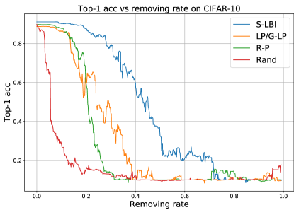
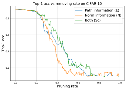
(a) Simplifying	(b) Different scores

Figure 8: (a) Comparison of simplifying ResNet-20 in CIFAR-10. X-axis and Y-axis represent the removing rate, and top-1 accuracy respectively. We can see that our $S^{2}$-LBI algorithm could beat all of our baseline models. (b) Pruning performance, if we only consider solution path (i.e.. $E$) or we only consider the magnitude of filters (i.e., $N$). The results are from the experiment in reducing all layers of Resnet-20 on CIFAR-10 dataset.

Simplifying more layers. We further conduct experiments of simplifying more layers of ResNet-20. Particularly, we train the network by $S^{2}$-LBI, and rank the importance of filters by Eq 10. The results are shown in Fig. 8(a). It shows that our simplified network has much better results than others; this again, demonstrates the efficacy of $S^{2}$-LBI in efficiently and selectively training the network. Note that, the ResNet-20 is relatively a compact structure of learning data in CIFAR-10; thus with the pruning rate beyond $20\%$, all methods get degraded dramatically.

5.3 Ablation Study

Simplifying criterion. The score of filters are weighted by the vector $E$ of first selecting one filter, and magnitude value vector $M$ of each filter at the converged epoch, as Eq 10. On CIFAR-10, we use the ResNet-20 as the backbone, and simplifying the network by using $E$, $M$ or $Sc$ (Eq 10). The results are shown in Fig. 8. We remove the filters one by one. Clearly, it shows that by using either the path information ($E$), or the magnitude information ($M$), the network can still be efficiently simplified, again thanks to our $S^{2}$-LBI algorithm. Importantly, by combing both information, our algorithm can achieve better performance.

Visualization of Filters in Solution Path. We visualize the filters as the visualization algorithm Erhan et al. (2009) in order to show the filters learned by our $S^{2}$-LBI algorithm. On MNIST dataset, we train Lenet-5 network by using SGD with $L_{1}-$norm and $L_{2}-$norm on parameters. In contrast, we also employ our $S^{2}$-LBI to train the Lenet-5 structure. We visualize the conv.c5 filters of LeNet-5 in Fig. 7. We visualize the solution path in the left column, by comparing the changing of the magnitude of each filter with the training epochs. We use red color to represent the filters that have learned more obvious visual patterns. Particularly, in our $S^{2}$-LBI algorithm, the solution path of filters selected in $\widetilde{W}$ are drawn by red color. Thus, it is quite clear that both $S^{2}$-LBI and SGD with $L_{1}-$norm could produce a sparse DNN structure, and the magnitudes of most of filters are very small.

6 Conclusion

This paper proposes a $S^{2}$-LBI algorithm to train and boost the network, important filters at the same time. Particularly, the proposed algorithm, for the first time, can automatically grow or simplify a network. The experiments show the efficacy of proposed framework.

References

- Abbasi-Asl and Yu (2017) Reze Abbasi-Asl and Bin Yu. Structural compression of convolutional neural networks based on greedy filter pruning. In arxiv, 2017.
- Alvarez and Salzmann (2016) Jose M Alvarez and Mathieu Salzmann. Learning the number of neurons in deep networks. In NIPS, 2016.
- Bottou (2010) Léon Bottou. Large-scale machine learning with stochastic gradient descent. In COMPSTAT, 2010.
- Bühlmann and Yu (2003) Peter Bühlmann and Bin Yu. Boosting with the l2 loss: Regression and classification. Journal of the American Statistical Association, 98(462):324–339, 2003.
- Collins and Kohli (2014) Maxwell Collins and Pushmeet Kohli. Memory bounded deep convolutional networks. In arXiv preprint arXiv:1412.1442, 2014, 2014.
- Elsken et al. (2018) Thomas Elsken, Jan Hendrik Metzen, and Frank Hutter. Neural architecture search: A survey. In arxiv:1808.05377, 2018.
- Erhan et al. (2009) Dumitru Erhan, Yoshua Bengio, Aaron Courville, and Pascal Vincent. Visualizing higher-layer features of a deep network. University of Montreal, 1341(3):1, 2009.
- Han et al. (2015a) Song Han, Huizi Mao, and William J Dally. Deep compression: Compressing deep neural networks with pruning, trained quantization and huffman coding. In ICLR, 2015a.
- Han et al. (2015b) Song Han, Jeff Pool, John Tran, and William Dally. Learning both weights and connections for efficient neural network. In NIPS, 2015b.
- He et al. (2015) Kaiming He, Xiangyu Zhang, Shaoqing Ren, and Jian Sun. Delving deep into rectifiers: Surpassing human-level performance on imagenet classification. In ICCV, 2015.
- He et al. (2016) Kaiming He, Xiangyu Zhang, Shaoqing Ren, and Jian Sun. Deep residual learning for image recognition. In Proceedings of the IEEE conference on computer vision and pattern recognition, pages 770–778, 2016.
- Hinton et al. (2014) Geoffrey Hinton, Oriol Vinyals, and Jeff Dean. Distilling the knowledge in a neural network. In NIPS 2014 Deep Learning Workshop, 2014.
- Howard et al. (2017) Andrew G. Howard, Menglong Zhu, Bo Chen, Dmitry Kalenichenko, Weijun Wang, Tobias Weyand, Marco Andreetto, and Hartwig Adam. Mobilenets: Efficient convolutional neural networks for mobile vision applications. In arxiv, 2017.
- Huang et al. (2016a) Chendi Huang, Xinwei Sun, Jiechao Xiong, and Yuan Yao. Split lbi: An iterative regularization path with structural sparsity. advances in neural information processing systems. Advances In Neural Information Processing Systems, pages 3369–3377, 2016a.
- Huang et al. (2016b) Chendi Huang, Xinwei Sun, Jiechao Xiong, and Yuan Yao. Split lbi: An iterative regularization path with structural sparsity. In NIPS, pages 3369–3377, 2016b.
- Huang et al. (2018) Chendi Huang, Xinwei Sun, Jiechao Xiong, and Yao Yuan. Boosting with structural sparsity: A differential inclusion approach. Applied and Computational Harmonic Analysis, 2018.
- Iandola et al. (2017) Forrest N. Iandola, Song Han, Matthew W. Moskewicz, Khalid Ashraf, William J. Dally, and Kurt Keutzer. Squeezenet: Alexnet-level accuracy with 50x fewer parameters and ¡0.5mb model size. In ICLR, 2017.
- Jaderberg et al. (2014) Max Jaderberg, Andrea Vedaldi, and Andrew Zisserman. Speeding up convolutional neural networks with low rank expansions. In BMVC, 2014.
- Kingma and Ba (2015) Diederik Kingma and Jimmy Ba. Adam: A method for stochastic optimization. In ICLR, 2015.
- Krichene et al. (2015) Walid Krichene, Alexandre Bayen, and Peter L Bartlett. Accelerated mirror descent in continuous and discrete time. In Advances in neural information processing systems, pages 2845–2853, 2015.
- LeCun et al. (1998) Yann LeCun, Leon Bottou, Yoshua Bengio, and Patrick Haffner. Gradient-based learning applied to document recognition. 86(11):2278–2324, 1998.
- Li et al. (2017) Hao Li, Asim Kadav, Igor Durdanovic, Hanan Samet, and Hans Peter Graf. Pruning filters for efficient convnets. In ICLR, 2017.
- Li and Hoiem (2016) Zhizhong Li and Derek Hoiem. Learning without forgetting. In ECCV, 2016.
- Liu et al. (2017) Zhuang Liu, Jianguo Li, Zhiqiang Shen, Gao Huang, Shoumeng Yan, and Changshui Zhang. Learning efficient convolutional networks through network slimming. In ICCV, 2017.
- Ma et al. (2018) Ningning Ma, Xiangyu Zhang, Hai-Tao Zheng, and Jian Sun. Shufflenet v2: Practical guidelines for efficient cnn architecture design. In arXiv:1807.11164v1, 2018.
- Mason et al. (1999) Llew Mason, Jonathan Baxter, Peter Bartlett, and Marcus Frean. Boosting algorithms as gradient descent. In International Conference on Neural Information Processing Systems, 1999.
- Molchanov et al. (2017) Pavlo Molchanov, Stephen Tyree, Tero Karras, Timo Aila, and Jan Kautz. Pruning convolutional neural networks for resource efficient transfer learning. In ICLR, 2017.
- Osher et al. (2005) Stanley Osher, Martin Burger, Donald Goldfarb, Jinjun Xu, and Wotao Yin. An iterative regularization method for total variation-based image restoration. Multiscale Modeling & Simulation, 4(2):460–489, 2005.
- Osher et al. (2016) Stanley Osher, Feng Ruan, Jiechao Xiong, Yuan Yao, and Wotao Yin. Sparse recovery via differential inclusions. Applied and Computational Harmonic Analysis, 2016.
- Pentina and Lampert (2015) Anastasia Pentina and Christoph H. Lampert. Lifelong learning with non-i.i.d. tasks. In NIPS. 2015.
- Ranzato and Hinton (2010) M. Ranzato and G. E. Hinton. Modeling pixel means and covariances using factorized third-order boltzmann machines. In CVPR, 2010.
- Ranzato et al. (2010) M. Ranzato, A. Krizhevsky, and G. E. Hinton. Factored 3-way restricted boltzmann machines for modeling natural images. In AISTATS, 2010.
- Srivastava et al. (2014) Nitish Srivastava, Geoffrey Hinton, Alex Krizhevsky, Ilya Sutskever, and Ruslan Salakhutdinov. Dropout: a simple way to prevent neural networks from overfitting. The Journal of Machine Learning Research, 15(1):1929–1958, 2014.
- Sun et al. (2017) Xinwei Sun, Lingjing Hu, Yuan Yao, and Yizhou Wang. Gsplit lbi: Taming the procedural bias in neuroimaging for disease prediction. In International Conference on Medical Image Computing and Computer-Assisted Intervention, pages 107–115. Springer, 2017.
- Thrun and Mitchell (1995) Sebastian Thrun and Tom M. Mitchell. Lifelong robot learning. Robotics and Autonomous Systems, 1995.
- Wang et al. (2017) Yuxiong Wang, Deva Ramanan, and Martial Hebert. Growing a brain: Fine-tuning by increasing model capacity. In CVPR, 2017.
- Wen et al. (2016a) Wei Wen, Chunpeng Wu, Yandan Wang, Yiran Chen, and Hai Li. Learning the number of neurons in deep networks. In NIPS, 2016a.
- Wen et al. (2016b) Wei Wen, Chunpeng Wu, Yandan Wang, Yiran Chen, and Hai Li. Learning structured sparsity in deep neural networks. In NIPS, 2016b.
- Yang et al. (2018) He Yang, Guoliang Kang, Xuanyi Dong, Yanwei Fu, and Y. Yang. Soft filter pruning for accelerating deep convolutional neural networks. In IJCAI 2018, 2018.
- Yoon and Hwang (2017) Jaehong Yoon and Sung Ju Hwang. Combined group and exclusive sparsity for deep neural networks. In ICML, 2017.
- Yuan and Lin (2006) Ming Yuan and Yi Lin. Model selection and estimation in regression with grouped variables. Journal of the Royal Statistical Society: Series B (Statistical Methodology), 68(1):49–67, 2006.
- Yuan et al. (2007) Yao Yuan, Lorenzo Rosasco, and Andrea Caponnetto. On early stopping in gradient descent learning. Constructive Approximation, 26(2):289–315, 2007.
- Zhang et al. (2016) Xiangyu Zhang, Jianhua Zou, Kaiming He, and Jian Sun. Accelerating very deep convolutional networks for classification and detection. IEEE Transactions on Pattern Analysis and Machine Intelligence, 38(10):1943–1955, 2016.
- Zhao et al. (2018) Bo Zhao, Xinwei Sun, Yanwei Fu, Yuan Yao, and Yizhou Wang. Msplit lbi: Realizing feature selection and dense estimation simultaneously in few-shot and zero-shot learning. arXiv preprint arXiv:1806.04360, 2018.
- Zhou et al. (2017) Aojun Zhou, Anbang Yao, Yiwen Guo, Lin Xu, and Yurong Chen. Incremental network quantization: Towards lossless cnns with low-precision weights. ICLR, 2017.
- Zhu et al. (2017) Chenzhuo Zhu, Song Han, Huizi Mao, and William J Dally. Trained ternary quantization. ICLR, 2017.
- Zoph and Le (2016) Barret Zoph and Quoc V Le. Neural architecture search with reinforcement learning. arXiv preprint arXiv:1611.01578, 2016.