123456

Hasan, Van Hentenryck, and Legrain

The Commute Trip Sharing Problem

The Commute Trip Sharing Problem

Mohd. Hafiz Hasan University of Michigan, Ann Arbor, Michigan 48109, hasanm@umich.edu Pascal Van Hentenryck Georgia Institute of Technology, Atlanta, Georgia 30332, pascal.vanhentenryck@isye.gatech.edu Antoine Legrain Polytechnique Montréal, Montréal, Québec H3T 1J4, antoine.legrain@polymtl.ca

Parking pressure has been steadily increasing in cities as well as in university and corporate campuses. To relieve this pressure, this paper studies a car-pooling platform that would match riders and drivers, while guaranteeing a ride back and exploiting spatial and temporal locality. In particular, the paper formalizes the Commute Trip Sharing Problem (CTSP) to find a routing plan that maximizes ride sharing for a set of commute trips. The CTSP is a generalization of the vehicle routing problem with routes that satisfy time-window, capacity, pairing, precedence, ride-duration, and driver constraints. The paper introduces two exact algorithms for the CTSP: A Route-Enumeration Algorithm and a Branch-and-Price Algorithm. Experimental results show that, on a high-fidelity, real-world dataset of commute trips from a mid-size city, both algorithms optimally solve small and medium-sized problems and produce high-quality solutions for larger problem instances. The results show that car pooling, if widely adopted, has the potential to reduce vehicle usage by up to 57% and decrease vehicle miles traveled by up to 46% while only incurring a 22% increase in average ride time per commuter for the trips considered.

ride sharing; vehicle routing with time windows; column generation; branch and price; mixed-integer programming

1 Introduction

Parking occupies a significant portion of our cities. In the United States, for instance, there are at least 800 million parking spaces and, in Los Angeles County, 14% of the city space is devoted to parking (Taylor 2018). Parking also contributes to congestion: Based on a sample of 22 studies in the United States, the average share of traffic cruising to find a parking spot is 30% and the average cruising time is just under 8 minutes in downtown areas (Shoup 2005, 2006).

Parking pressure has also been steadily increasing in cities, university campuses, and corporations, alongside other concerns such as traffic congestion, fuel prices, and greenhouse gas emissions. In the city of Buffalo, New York, the overall supply of parking space has remained constant for the last 20 years, while the downtown population and the workforce have increased by 70% and 30% respectively (Epstein 2018). These parking shortages are perceived as an impediment to future economic developments, as corporations may elect to move elsewhere when growing their operations. University campuses feel similar parking pressures. For instance, Stanford University suffers from a lack of parking spaces due to construction and a growth in population (Chesley 2017). The research underlying this paper was originally motivated by parking pressure at the University of Michigan in Ann Arbor. Figure 1 depicts the parking utilization of the 15 most used parking lots in downtown Ann Arbor. They show a typical parking usage: Cars arrive in the morning, park in the lot for 6 to 10 hours, and leave the lot in the evening.

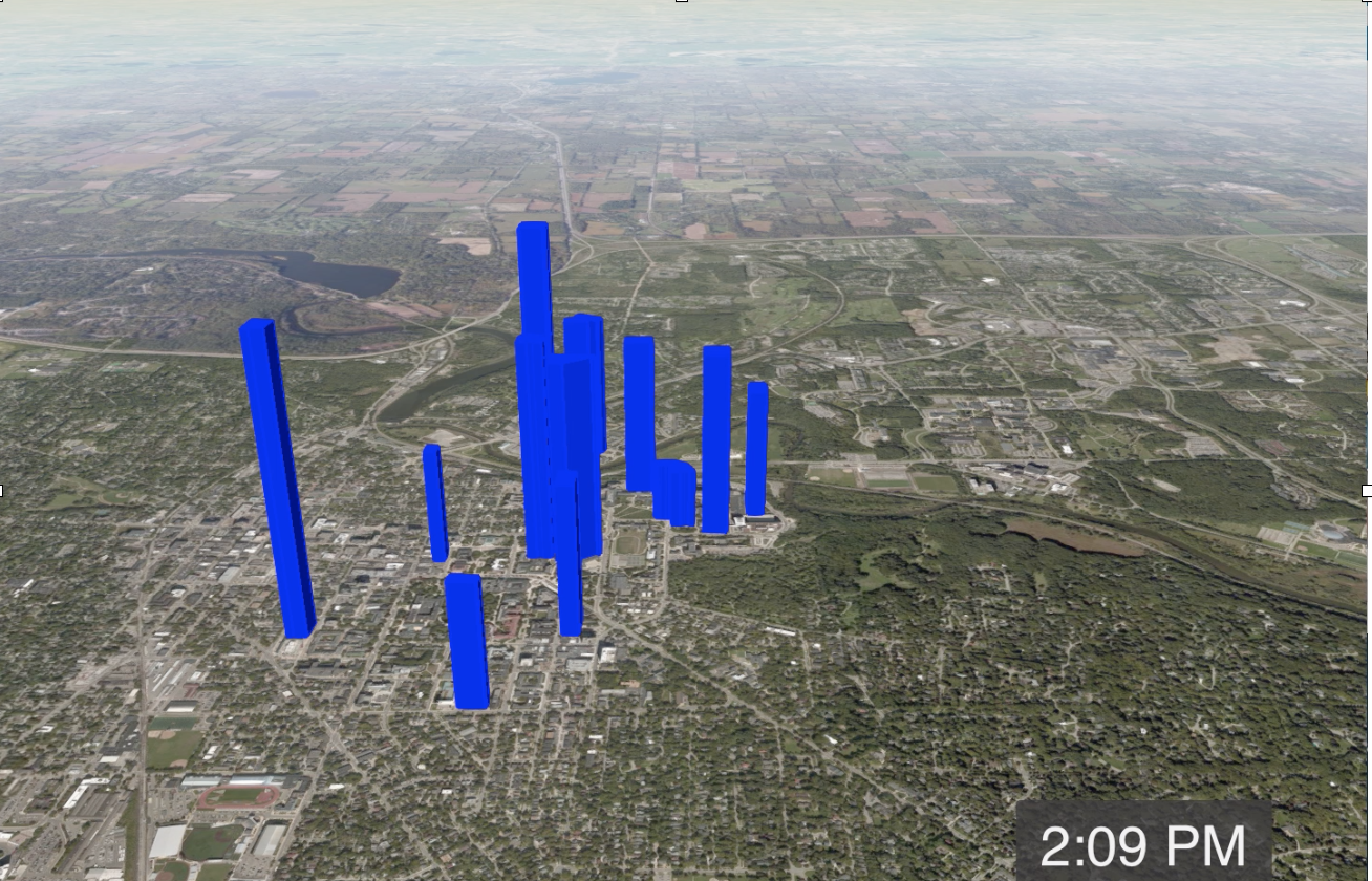
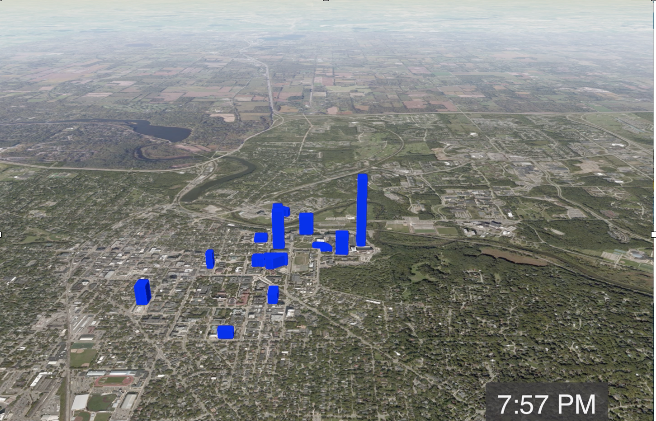
Figure 1: The Main University Parking Lots in Downtown Ann Arbor.

To address the increasing demand on these lots, we started to investigate the potential of a community-based car-pooling program (Hasan et al. 2018). The idea was to implement a car-pooling program organized around the communities commuting to the university, exploiting the knowledge of when employees were arriving in the morning and leaving in the evening. However, while car-pooling has long been proposed as a solution to reduce peak-hour congestion and parking utilization, its adoption in the US remains poor as 76.4% of American commuters chose to drive alone according to the 2013 American Community Survey (McKenzie 2015). A study on factors influencing carpool formation by Li et al. (2007) revealed difficulty in finding people with the same location and schedule as the primary reason for not carpooling. As a result, we investigated how to alleviate this burden and studied the feasibility of a matching platform that would automatically identify commuting groups based on factors determined to be consequential to individuals’ commuting decisions. One of the results of our study was the recognition that an effective car-pooling platform will need to accommodate different sharing patterns for every weekday and, as a result, the platform will need to optimize trip matching on a daily basis to allow significant car pooling to occur (Hasan et al. 2018).

The goal of this paper is to propose, and analyze, scalable optimization algorithms for powering such a platform. A meta-analysis of related work reveals that car-pooling and car-sharing platforms should at least implement the following three guiding principles:

1. Spatial proximity of riders (Richardson and Young 1981, Buliung et al. 2009);

2. Temporal proximity of riders (Tsao and Lin 1999, Buliung et al. 2010, Poulenez-Donovan and Ulberg 1994);

3. Guaranteed ride back home (Correia and Viegas 2011).

The first two guidelines are natural since car-pooling is unlikely to occur for riders who are not close spatially or whose schedules are not compatible. The third guideline is critical: It is unlikely that many riders will use a platform that does not guarantee a ride back home in the evening. The guarantee of a ride back home is one of the main contributions of this work: For instance, the car-pooling platform Scoop provides only weak guarantees for “ride back” and with monthly limits on how much auxiliary services can be used when a ride back is not available. In contrast, this paper approaches the matching of riders in two steps. In the first step, riders are grouped spatially into neighborhoods using a clustering algorithm. In the second step, an optimization algorithm selects drivers and matches riders to minimize the number of cars and the total travel distance. The approach follows the three guiding principles listed above and, in particular, ensures that every rider has a guaranteed ride back. The contributions of this paper are threefold.

1. It first defines the Commute Trip Sharing Problem (CTSP) that formally captures the matching problem described previously.

2. It proposes two algorithms, a Route-Enumeration Algorithm and a Branch-and-Price Algorithm, to solve the CTSP for a cluster of riders.

3. It analyzes the scalability of the two algorithms along different dimensions, including the capacity of the vehicles, the size of the clusters, and their ability to be deployed in real situations.

The CTSP can be viewed as a generalization of the Vehicle Routing Problem (VRP) with routes satisfying time-window, capacity, pairing, precedence, ride-duration, and driver constraints. In addition to picking up and dropping off riders within desired time windows while ensuring vehicle capacities are not exceeded, routes in the CTSP must also ensure their ride durations are not excessively long to limit user inconvenience. In this sense, the CTSP shares some similarities with the Dial-a-Ride Problem (DARP). It differs from the DARP in that it relies on the use of personal vehicles to serve all trip requests, which come in pairs for each commuter as each rider makes a trip to the workplace and another back home. The drivers of these vehicles therefore belong the set of riders, and their routes to the workplace and back home must be carefully constructed and balanced to ensure that every rider is covered on their way to work and guaranteed a ride back home. These additional requirements make the CTSP unique and particularly challenging. The CTSP also uses a lexicographic objective function that first minimizes the number of cars and then the total travel distance.

The paper proposes two exact algorithms for the CTSP: A Route-Enumeration Algorithm (REA) which exhaustively searches for feasible routes from all possible trip combinations before route selection is optimized with a mixed-integer program (MIP), and a Branch-and-Price algorithm (BPA) which uses column generation and a pricing algorithm based on dynamic programming. On top of the two algorithms, the paper highlights key characteristics of the CTSP differentiating it from the DARP that allow its routes to be enumerated by the REA. While the BPA builds on conventional techniques to solve the CTSP via column generation, it introduces a wait-time relaxation technique, which is a novel alternative to the weak and strong dominance relations proposed by Gschwind and Irnich (2015) for finding feasible routes that simultaneously satisfy time-window and ride-duration constraints in the pricing problem. The paper also proposes a time-limited, root-node heuristic which is derived from the BPA and demonstrates its capability to produce high-quality solutions for medium to large problem instances within a 10-minute time span, making it well suited for time-constrained scenarios within an operational setting. Finally, the paper proposes a clustering algorithm to decompose large-scale problems by spatially grouping commuters based on their home locations, which is then used to generate problem instances for evaluating the algorithms from a real-world dataset of commute trips from the city of Ann Arbor, Michigan.

The remainder of this paper is organized as follows. The next section first briefly reviews relevant literature, and it is followed by Section 3 which introduces the terminology and assumptions used throughout this work. Section 4 then provides a formal definition and a mathematical formulation of the CTSP, followed by Section 5 which introduces the first algorithm to solve the problem, the REA. Next, Section 6 describes the second algorithm, the BPA together with its derived root-node heuristic, while the clustering algorithm is presented in Section 7. Lastly, computational results are reported in Section 8, after which concluding remarks are provided in Section 9.

2 Related Work

The Vehicle Routing Problem with Time Windows (VRPTW) seeks a set of minimum-cost routes for a fleet of vehicles that start and end at a central depot. The routes serve a set of customers with specific demands and time windows describing allowable service times, and they must ensure that each customer is served exactly once and the capacity of the vehicles are not exceeded. The problem has been widely studied in the literature and is known to be NP-hard, since finding a solution for a fixed fleet has been shown to be NP-complete (Savelsbergh 1985). Nevertheless, various methods, from metaheuristics like Taillard et al. (1997) and Bräysy and Gendreau (2005) to exact solution approaches based on Lagrangian relaxation (Kohl and Madsen 1997, Kallehauge et al. 2006) or column generation (Desrochers et al. 1992, Kohl et al. 1999), have been proposed to efficiently solve it. An extensive review of the problem may be obtained from Cordeau et al. (2002).

Dumas et al. (1991) introduced the Pickup and Delivery Problem with Time Windows (PDPTW) to satisfy transportation requests requiring both pickup and delivery. It generalizes the VRPTW by introducing additional pairing and precedence constraints that require each route to serve the pickup location before the delivery location of the same customer, and it is solved using a column generation algorithm which utilizes dynamic programming to solve its pricing subproblem. The DARP, which is commonly used to model door-to-door transportation services for the disabled and the elderly, builds upon the PDPTW by introducing ride-duration limit constraints for each customer. As humans are being transported in the DARP instead of goods, customer ride time becomes an essential quality of service criterion. Methods proposed to solve small and medium-sized instances of the problem include heuristics (Jaw et al. 1986, Bodin and Sexton 1986), metaheuristics (Cordeau and Laporte 2003b, Ritzinger et al. 2016), and exact algorithms (Cordeau 2006, Gschwind and Irnich 2015). The problem has also been extensively surveyed by Cordeau and Laporte (2003a) and Cordeau and Laporte (2007).

When column generation is used to solve the various generalizations of the VRPTW, its pricing subproblem typically involves solving an Elementary Shortest Path Problem with Resource Constraints (ESPPRC). Since the problem has been proven to be NP-hard in the strong sense by Dror (1994), most works have resorted to relaxing the elementary path requirement to result in a Shortest Path Problem with Resource Constraints (SPPRC) which admits a pseudo-polynomial algorithm. Non-elementary paths are then tackled using various methods; for instance, Desrosiers et al. (1984) and Dumas et al. (1991) have them eliminated in the integer solution of the restricted master problem, while Desrochers et al. (1992) and Irnich and Villeneuve (2006) opted for a middle ground approach by performing $2$- and $k$-cycle elimination respectively. Exact algorithms have also been proposed for solving the ESPPRC, e.g. by Feillet et al. (2004) and Chabrier (2006). Popular methods for solving the SPPRC and ESPPRC utilize dynamic programming, for instance the label-correcting algorithm of Desrosiers et al. (1983) which is based on the Ford-Bellman-Moore algorithm, the label-setting algorithm of Desrochers and Soumis (1988) which generalizes Dijktra’s algorithm, or the generalized label-setting algorithm for multiple resource constraints of Desrochers (1988). Methods using Lagrangian relaxation (e.g., Beasley and Christofides (1989), Borndörfer et al. (2001)) or constraint programming (e.g., Rousseau et al. (2004)) have also been explored. An in-depth overview of the SPPRC is provided by Irnich and Desaulniers (2005).

More recently, the availability of large-scale datasets like the New York City (NYC) Taxi and Limousine Commission (TLC) trip record, which contains data for over 1 billion taxi trips in NYC recorded since January 2009, has driven research towards ride sharing for on-demand transportation. For instance, Santi et al. (2014) introduced the notion of shareability graphs in an attempt to quantify the benefits of sharing these taxi rides. Alonso-Mora et al. (2017) then built upon the shareability graph idea to mathematically model the on-demand ride sharing problem and propose an anytime optimal algorithm to solve it. Agatz et al. (2012) provided an overview of planning considerations and issues of dynamic ride-sharing, classified different variations of ride-sharing problems, including single- and multi-modal versions, and reviewed related optimization models and approaches to address them. On the other hand, Mourad et al. (2019) took a broader view of shared mobility and surveyed optimization approaches for a wider range of applications, from prearranged to real-time problem settings that even includes combined transportation of people and freight. To our knowledge, Hasan et al. (2018) are the first to focus vehicle routing optimization on commute trips. They introduced the CTSP, explored the performance of various optimization models that enforce different sets of driver and commuter matching constraints, and discovered that commuter matching flexibility, i.e., their willingness to be matched with different drivers and passengers daily, is key for an effective ride-sharing platform. This paper extends their work by first refining their best performing ride-sharing model, introducing two algorithms to optimize the model, and performing an extensive comparative analysis of both algorithms using a high-fidelity, real-world dataset.

3 Notation and Preliminaries

A trip $t=<o,dt,d,at>$ consists of an origin $o$, a desired departure time $dt$, a destination $d$, and a desired arrival time $at$. On any day, a commuter $c$ makes two trips: a trip to the workplace, $t_{c}^{+}$, and a trip back home, $t_{c}^{-}$. These trips are referred to henceforth as inbound and outbound trips respectively. A route $r$ is a sequence of origin and destination locations from a set of inbound or outbound trips whereby each origin and destination from the set is visited exactly once. For instance, a possible route for trips $t_{1}=<o_{1},dt_{1},d_{1},at_{1}>$ and $t_{2}=<o_{2},dt_{2},d_{2},at_{2}>$ is $r=o_{2}\rightarrow o_{1}\rightarrow d_{1}\rightarrow d_{2}$. An inbound route covers only inbound trips and an outbound route covers only outbound trips. Each route $r$ serves a set of riders $\mathcal{C}_{r}$ and has a driver $D_{r}\in\mathcal{C}_{r}$. The driver must be the rider residing at the start location of the route. For instance, commuter 2 must be the driver of route $o_{2}\rightarrow o_{1}\rightarrow d_{1}\rightarrow d_{2}$. The total number of riders in the vehicle at any point along a route cannot exceed its capacity.

Definition 3.1 (Valid Route)

A valid route $r$ visits $o_{c}$ before $d_{c}$ for every rider $c\in\mathcal{C}_{r}$, starts at $o_{D_{r}}$ and ends at $d_{D_{r}}$, and respects the vehicle capacity.

The paper assumes that commuters sharing rides are willing to tolerate some inconvenience in terms of deviations to their trips’ desired departure and arrival times as well as in terms of extensions to the ride durations of their individual trips. Therefore, a time window $[a_{i},b_{i}]$ is constructed around the desired times and is associated with each pickup or drop-off location $i$, where $a_{i}$ and $b_{i}$ denote the earliest and latest times at which service may begin at $i$ respectively, and a duration limit $L_{c}$ is associated with each commuter $c$ to denote her maximum ride duration. In this paper, $T_{i}$ denotes the time at which service begins at location $i$, $s_{i}$ is the service duration at $i$, $pred(i)$ denotes the location on a route visited just before $i$, and $\tau_{(i,j)}$ is the estimated travel time for the shortest path between locations $i$ and $j$.

Definition 3.2 (Feasible Route)

A feasible route $r$ is a valid route that has pickup and drop-off times $T_{i}\in[a_{i},b_{i}]$ for each location $i\in r$ and ensures the ride duration of each commuter $c\in\mathcal{C}_{r}$ does not exceed $L_{c}$.

$$\min \quad T_{d_{D_{r}}}-T_{o_{D_{r}}}$$ (1)

s.t.

$$\quad a_{o_{c}}\leq T_{o_{c}}\leq b_{o_{c}}\qquad\forall c\in\mathcal{C}_{r}$$ (2)

$$\quad T_{d_{c}}\leq b_{d_{c}}\qquad\forall c\in\mathcal{C}_{r}$$ (3)

$$\quad T_{pred(o_{c})}+s_{pred(o_{c})}+\tau_{(pred(o_{c}),o_{c})}\leq T_{o_{c}}\qquad\forall c\in\mathcal{C}_{r}\setminus\{D_{r}\}$$ (4)

$$\quad T_{pred(d_{c})}+s_{pred(d_{c})}+\tau_{(pred(d_{c}),d_{c})}=T_{d_{c}}\qquad\forall c\in\mathcal{C}_{r}$$ (5)

$$\quad T_{d_{c}}-(T_{o_{c}}+s_{o_{c}})\leq L_{c}\qquad\forall c\in\mathcal{C}_{r}$$ (6)

Determining if a valid route $r$ is feasible amounts to solving the route-scheduling problem of (1)–(6). Its objective is to minimize the total duration of the route. Constraints (2) and (3) are time-window constraints for pickup and drop-off locations respectively, while constraints (4) and (5) describe compatibility requirements between pickup/drop-off times and travel times between consecutive locations along the route. Finally, constraints (6) specify the ride-duration limit for each rider. Note that constraints (4) allow waiting at pickup locations, and constraints (2) and (3) implicitly limit the trip duration of rider $c$ by $(b_{d_{c}}-a_{o_{c}})$.

The route validity requirement specifies route structural constraints which enforce pairing and precedence of origins and destinations, vehicle capacity, and the driver role, whereas the feasibility requirement specifies time-window and ride-duration limit constraints which are temporal in nature in addition to those for route validity. Lastly, this work assumes utilization of a homogeneous fleet of vehicles with capacity $K$ to serve all trips, and that all travel times and distances satisfy the triangle inequality.

4 The Commute Trip Sharing Problem

The CTSP aims at finding a set of minimum-cost feasible routes to cover all inbound and outbound trips of a set of commuters $\mathcal{C}$ while ensuring the set of drivers for inbound and outbound routes are identical. Let $\Omega^{+}$ and $\Omega^{-}$ denote the set of all feasible inbound and outbound routes respectively, and $c_{r}$ denote the cost of route $r$. The CTSP formulation uses a binary variable $X_{r}$ to indicate whether a route $r\in\Omega^{+}\cup\Omega^{-}$ is selected, a binary constant $\alpha_{r,i}$ which is equal to 1 iff route $r$ serves rider $i$ (i.e., $\alpha_{r,i}=1$ iff $i\in\mathcal{C}_{r}$), and a binary constant $\beta_{r,i}$ which is equal to 1 iff rider $i$ is the driver of route $r$ (i.e., $\beta_{r,i}=1$ iff $i=D_{r}$). The problem formulation is given by (7)–(11).

$$\min \quad\sum_{r\in\Omega^{+}\cup\Omega^{-}}c_{r}X_{r}$$ (7)

s.t.

$$\quad\sum_{r\in\Omega^{+}}\alpha_{r,i}X_{r}=1\qquad\forall i\in\mathcal{C}$$ (8)

$$\quad\sum_{r\in\Omega^{-}}\alpha_{r,i}X_{r}=1\qquad\forall i\in\mathcal{C}$$ (9)

$$\quad\sum_{r\in\Omega^{+}}\beta_{r,i}X_{r}-\sum_{\hat{r}\in\Omega^{-}}\beta_{\hat{r},i}X_{\hat{r}}=0\qquad\forall i\in\mathcal{C}$$ (10)

$$\quad X_{r}\in\{0,1\}\qquad\forall r\in\Omega^{+}\cup\Omega^{-}$$ (11)

The model features a lexicographic objective that first minimizes the number of cars and then the total distance. It is rewritten into a single objective by appropriate weighting of the two sub-objectives. The cost $c_{r}$ penalizes the total distance of route $r$ and heavily penalizes its selection. Let $\delta_{(i,j)}$ denote the distance of the shortest path between nodes $i$ and $j$. $c_{r}$ is then given by the addition of variable and fixed costs of the route:

$$c_{r}=\hat{c}_{r}+\bar{c}$$ (12)

where the variable and fixed costs, $\hat{c}_{r}$ and $\bar{c}$, are given by:

$$\hat{c}_{r}=\sum_{(i,j)\in r}\delta_{(i,j)}$$ (13)

$$\bar{c}=M\max_{r\in\Omega^{+}\cup\Omega^{-}}{\sum_{(i,j)\in r}\delta_{(i,j)}}$$ (14)

where $M$ is a large number. In practice, $M$ is set to 1000, which is sufficiently large to ensure that the number of selected routes is first minimized followed by their total distance. Constraints (8) and (9) enforce coverage of each rider’s inbound and outbound trips by exactly one route each, while constraints (10) ensure drivers of inbound and outbound routes are identical. The set-partitioning problem of (7)–(11) is referred to as the master problem (MP) from this point forth.

The CTSP is essentially a vehicle routing problem with driver, capacity, time-window, pairing, precedence, ride-duration, and driver constraints, making it most similar to the DARP. However, the key distinctions of the CTSP are:

1. Drivers in the CTSP are members of the set of riders, i.e., $D_{r}\in\mathcal{C}_{r}$. This leads to driver constraints which require routes to start and end at the drivers’ origins and destinations respectively, whereas requests in the DARP are served by shared vehicles whose routes begin and end at a central depot.

2. The set of drivers for inbound and outbound routes needs to be balanced, leading to constraints (10) in the MP. These constraints add another layer of complexity which is not present in the DARP.

Therefore, the CTSP can also be seen as a DARP with additional constraints.

5 The Route-Enumeration Algorithm

One approach to solve the CTSP is by enumerating all routes in $\Omega^{+}\cup\Omega^{-}$ before solving the MP with a MIP solver. The REA supports this approach by exhaustively searching for these routes from all possible trip combinations. Let $\mathcal{T}^{+}$ and $\mathcal{T}^{-}$ denote all inbound and outbound trips taken by the set of commuters $\mathcal{C}$ respectively, i.e., $\mathcal{T}^{+}=\{\,t_{c}^{+}\,:\,c\in\mathcal{C}\,\}$ and $\mathcal{T}^{-}=\{\,t_{c}^{-}\,:\,c\in\mathcal{C}\,\}$. Without loss of generality, Algorithm 1 summarizes how $\Omega^{+}$ is obtained from $\mathcal{T}^{+}$ using a homogeneous fleet of vehicles with capacity $K$.

Routes of all individual trips from $\mathcal{T}^{+}$ are first added to $\Omega^{+}$ (lines 2–3). To obtain feasible routes covering more than 1 trip, an index $k$ is first set to the number of shared trips desired, after which all $k$-combinations of trips from $\mathcal{T}^{+}$ (denoted by $\mathcal{Q}_{k}$) are enumerated (lines 4–5). For each trip combination $q\in\mathcal{Q}_{k}$, the set of valid routes for the combination is then enumerated. For instance, let $k=2$, $q=\{t_{1},t_{2}\}$, and $t_{1}=<o_{1},dt_{1},d_{1},at_{1}>$ and $t_{2}=<o_{2},dt_{2},d_{2},at_{2}>$. The set of valid routes for $q$ is $\{\,o_{1}\rightarrow o_{2}\rightarrow d_{2}\rightarrow d_{1},\,o_{2}\rightarrow o_{1}\rightarrow d_{1}\rightarrow d_{2}\,\}$. $\Omega^{v}_{q}$ denotes the set of all valid routes for $q$ and $\mathcal{C}_{q}$ denotes the set of all riders making the trips in $q$.

Algorithm 1 Route-Enumeration Algorithm for $\Omega^{+}$

1:$\mathcal{T}^{+},K$

2:$\Omega^{+}\leftarrow\text{\O}$

3:for each $t_{c}^{+}\in\mathcal{T}^{+}$ do

4:     $\Omega^{+}\leftarrow\Omega^{+}\cup\{o_{c}^{+}\rightarrow d_{c}^{+}\}$

5:for $k=2$ to $K$ do

6:     $\mathcal{Q}_{k}\leftarrow\{$all $k$-combinations of $\mathcal{T}^{+}\}$

7:     for each $q\in\mathcal{Q}_{k}$ do

8:         $\Omega^{v}_{q}\leftarrow\{$all valid routes of $q\}$

9:         for each $c\in\mathcal{C}_{q}$ do

10:              $\Omega_{\text{temp}}\leftarrow\text{\O}$

11:              for each $r\in\Omega^{v}_{q}\,:\,D_{r}=c$ do

12:                  if $feasible(r)$ then

13:                       $\Omega_{\text{temp}}\leftarrow\Omega_{\text{temp}}\cup\{r\}$                                 

14:              $\Omega^{+}\leftarrow\Omega^{+}\cup\{\argmin_{r\in\Omega_{\text{temp}}}\sum_{(i,j)\in r}\delta_{(i,j)}\}$               

15:return $\Omega^{+}$

The algorithm then iterates over every rider $c\in\mathcal{C}_{q}$ and considers only routes in $\Omega^{v}_{q}$ where $c$ is the driver, i.e., $\{r\in\Omega^{v}_{q}\,:\,D_{r}=c\}$ (lines 8–10). A function $feasible(r)$, which solves the route-scheduling problem of (1)–(6) on route $r$ and returns a Boolean value indicating whether $r$ is feasible, is then utilized to identify feasible routes to be stored in a temporary set $\Omega_{\text{temp}}$. Only the route with the shortest travel distance from $\Omega_{\text{temp}}$ is then added to $\Omega^{+}$ (line 13). Note that this step is optional. It is done to reduce the size of $\Omega^{+}$ with the knowledge that only one route may be selected for each driver covering $\mathcal{C}_{q}$ in a feasible solution to the MP. The route with minimal travel distance is chosen knowing that the secondary objective of the MP is to minimize the total distance of selected routes.

In practice, the search procedure in lines 7–13 may be executed more efficiently via a depth-first search implementation which uses the length of the best feasible route to prune the search space and through parallel execution of the search procedure for all $q\in\mathcal{Q}_{k}$ since they are independent of each other. The procedure of exploring all $k$-combinations is repeated with increasing values of $k$ from 2 up to the vehicle capacity $K$ to completely enumerate $\Omega^{+}$. $\Omega^{-}$ is obtained by repeating the algorithm on $\mathcal{T}^{-}$.

The fact that drivers are commuters themselves is the key characteristic of the CTSP: It allows its routes to be exhaustively enumerated. Indeed, drivers must complete their trips within their time windows and, most importantly, their trips are subject to ride-duration constraints. As a result, in general, a route typically consists of three phases: A pickup phase where the driver picks up passengers, a driving phase where the vehicle travels to the destination, and a drop-off phase where the driver drops off all the passengers before ending her trip. After the drop-offs, the driver has no time to go back and pick up another set of passengers due to her time-window and ride-duration constraints. This permits the REA to consider only routes that contain up to $k\leq K$ passengers (line 4 in Algorithm 1) to enumerate all possible routes, and $K$ is typically small. In contrast, the DARP uses dedicated drivers who are not subject to any ride-duration constraints and can serve riders throughout the day. Therefore it cannot restrict attention to routes with only $k\leq K$ passengers: The number of passengers in a route is not limited by the capacity of the vehicle, but by the total number of travelers.

6 The Branch-and-Price Algorithm

The BPA combines existing techniques with some novel elements to solve the CTSP. At its core is a conventional column-generation algorithm which utilizes a restricted master problem (RMP)—the linear relaxation of the MP defined on a subset of all feasible routes $\Omega^{+\prime}\cup\Omega^{-\prime}$—and solves a pricing subproblem (PSP) to identify new feasible routes with negative reduced costs. The PSP solves several dynamic programs that search for resource-constrained shortest paths representing the feasible routes. A bi-level branching strategy tailored specifically for the CTSP is then employed for obtaining integer solutions.

This work introduces a novel wait-time relaxation technique that not only obtains feasible routes that simultaneously satisfy time-window and ride-duration constraints in the PSP, but also guarantees elementarity of the routes. It proposes utilization of a resource that models trip durations excluding wait times which allow the dynamic programs to produce preliminary routes with minimal reduced costs that first satisfy a set of constraints necessary for route feasibility. The feasibility of the preliminary routes are then evaluated with the inclusion of wait times, and infeasible ones are added to a set of forbidden paths whose members are prevented from subsequent discovery via the dynamic-programming approach of Di Puglia Pugliese and Guerriero (2013a).

6.1 The Pricing Subproblem

The PSP is responsible for finding new feasible routes with negative reduced costs. Letting $\pi_{i}^{+}$, $\pi_{i}^{-}$, and $\sigma_{i}$ denote the optimal duals of constraints (8), (9), and (10) of the RMP respectively, the reduced cost of an inbound route $r^{+}$ is given by:

$$rc_{r^{+}}=c_{r^{+}}-\sum_{i\in\mathcal{C}_{r^{+}}}\pi_{i}^{+}-\sigma_{D_{r^{+}}}$$ (15)

while that of an outbound route $r^{-}$ is given by:

$$rc_{r^{-}}=c_{r^{-}}-\sum_{i\in\mathcal{C}_{r^{-}}}\pi_{i}^{-}+\sigma_{D_{r^{-}}}$$ (16)

These routes are obtained by considering each rider $d\in\mathcal{C}$ as the driver of an inbound route $r_{d}^{+}$ and an outbound route $r_{d}^{-}$, and then finding such routes with minimum reduced costs. To obtain these routes, the algorithm builds a pair of graphs $\mathcal{G}_{d}^{+}$ and $\mathcal{G}_{d}^{-}$ for each $d\in\mathcal{C}$. In the following, $\mathcal{G}$ denotes the set of all constructed graphs, i.e., $\mathcal{G}=\{\mathcal{G}_{d}^{+}\,:\,d\in\mathcal{C}\}\cup\{\mathcal{G}_{d}^{-}\,:\,d\in\mathcal{C}\}$. Without loss of generality, the presentation outlines how a route $r_{d}^{+}$ with minimal reduced cost is found from $\mathcal{G}_{d}^{+}$.

First, let $n=|\mathcal{C}|$, and $\mathcal{O}^{+}=\{1,\cdots,n\}$ and $\mathcal{D}^{+}=\{n+1,\cdots,2n\}$ denote the sets of all origin and destination nodes respectively. The origin and destination of rider $i$ are then represented by nodes $i$ and $n+i$ respectively. The graph $\mathcal{G}_{d}^{+}=\{\mathcal{N}_{d}^{+},\mathcal{A}_{d}^{+}\}$ is built with nodes $\mathcal{N}_{d}^{+}=\mathcal{O}^{+}\cup\mathcal{D}^{+}$ and fully-connected edges $\mathcal{A}_{d}^{+}$. A ride-duration limit $L_{i}$ and a demand $\kappa_{i}$, representing the number of riders to be picked up at node $i$, are then associated with each node $i\in\mathcal{O}^{+}$, a time window $[a_{i},b_{i}]$ and a service duration $s_{i}$ are associated with each node $i\in\mathcal{N}_{d}^{+}$, and a travel time $\tau_{(i,j)}$ and a reduced cost $c_{(i,j)}$ are associated with each edge $(i,j)\in\mathcal{A}_{d}^{+}$. Letting $\gamma^{+}(i)$ and $\gamma^{-}(i)$ denote the set of outgoing and incoming edges of node $i$, the edge costs are defined as follows so that the total cost of any path from $d$ to $n+d$ is equivalent to $rc_{r_{d}^{+}}$:

$$c_{(i,j)}=\begin{cases}\bar{c}+\delta_{(i,j)}-\pi_{i}^{+}-\sigma_{d}&\qquad\forall(i,j)\in\gamma^{+}(d)\\ \delta_{(i,j)}-\pi_{i}^{+}&\qquad\forall i\in\mathcal{O}^{+}\setminus\{d\},\,\forall(i,j)\in\gamma^{+}(i)\\ \delta_{(i,j)}&\qquad\forall i\in\mathcal{D}^{+},\,\forall(i,j)\in\gamma^{+}(i)\end{cases}$$ (17)

Similarly, letting $\mathcal{O}^{-}$ and $\mathcal{D}^{-}$ denote the sets of all outbound origin and destination nodes, the graph $\mathcal{G}_{d}^{-}=\{\mathcal{N}_{d}^{-},\mathcal{A}_{d}^{-}\}$ is built with nodes $\mathcal{N}_{d}^{-}=\mathcal{O}^{-}\cup\mathcal{D}^{-}$ and fully-connected edges $\mathcal{A}_{d}^{-}$, and the costs of edges $(i,j)\in\mathcal{A}_{d}^{-}$ are defined as follows to ensure the total cost of any path from $d$ to $n+d$ in $\mathcal{G}_{d}^{-}$ is equal to $rc_{r_{d}^{-}}$:

$$c_{(i,j)}=\begin{cases}\bar{c}+\delta_{(i,j)}-\pi_{i}^{-}+\sigma_{d}&\qquad\forall(i,j)\in\gamma^{+}(d)\\ \delta_{(i,j)}-\pi_{i}^{-}&\qquad\forall i\in\mathcal{O}^{-}\setminus\{d\},\,\forall(i,j)\in\gamma^{+}(i)\\ \delta_{(i,j)}&\qquad\forall i\in\mathcal{D}^{-},\,\forall(i,j)\in\gamma^{+}(i)\end{cases}$$ (18)

A priori feasibility constraints, further detailed in Section 6.2, are then applied to identify and eliminate edges that cannot belong to any feasible route. Figure 6.1 provides a sketch of $\mathcal{G}_{d}^{+}$ after application of several of these edge elimination rules.

Graph $\mathcal{G}_{d}^{+}$ After Application of Edge Elimination Rules (a) and (b) from Section 6.2 (Each Dotted Line Represents a Pair of Bidirectional Edges).

The minimum-reduced-cost $r_{d}^{+}$ is then obtained by finding the least-cost feasible path from $d$ to $n+d$ in $\mathcal{G}_{d}^{+}$. Recall that for the path to be feasible, it must satisfy the time-window, capacity, pairing, precedence, ride-duration and driver constraints. The problem is therefore an Elementary Shortest Path Problem with Resource Constraints (ESPPRC) which is known to be NP-hard (Dror 1994). While the driver constraint is enforced by construction by making $d$ the source and $n+d$ the target of the shortest-path problem, the remaining constraints are implemented by introducing and enforcing constrained resources in a resource-constrained shortest path algorithm (RCSPA) which is further elaborated in Section 6.3. On the whole, the PSP involves solving $2n$ independent ESPPRCs to produce up to $2n$ feasible routes with negative reduced costs.

6.2 Time Windows Tightening and Edge Elimination

Pre-processing of the time-window, precedence, pairing, capacity, ride-duration limit, and driver constraints makes it possible to identify edges that cannot belong to any feasible route which may then be removed from $\mathcal{G}$. Without loss of generality, the following description focuses on edge elimination for $\mathcal{G}_{d}^{+}$.

Prior to determining infeasible edges, the time windows of all nodes are tightened by sequentially reducing their upper and lower bounds using the following rules introduced by Dumas et al. (1991).

• $b_{i}=\min\{b_{i},b_{n+d}-s_{i}-\tau_{(i,n+d)}\},\,\forall i\in\mathcal{D}^{+}\setminus\{n+d\}$

• $b_{i}=\min\{b_{i},b_{n+i}-s_{i}-\tau_{(i,n+i)}\},\,\forall i\in\mathcal{O}^{+}\setminus\{d\}$

• $a_{i}=\max\{a_{i},a_{d}+s_{d}+\tau_{(d,i)}\},\,\forall i\in\mathcal{O}^{+}\setminus\{d\}$

• $a_{i}=\max\{a_{i},a_{i-n}+s_{i-n}+\tau_{(i-n,i)}\},\,\forall i\in\mathcal{D}^{+}\setminus\{n+d\}$

The following constraints and rules, derived by combining those proposed by Dumas et al. (1991) and Cordeau (2006), are then applied to identify and eliminate infeasible edges:

1. Driver: Edges $\{(d,n+i),(i,d),(i,n+d),(n+i,d),(n+d,i),(n+d,n+i)\,:\,i\in\mathcal{O}^{+}\setminus\{d\}\}$.

2. Pairing and precedence: Edges $\{(n+i,i)\,:\,i\in\mathcal{O}^{+}\}$.

3. Capacity: Edges $\{(i,j),(j,i),(i,n+j),(j,n+i),(n+i,n+j),(n+j,n+i)\,:\,i,j\in\mathcal{O}^{+}\wedge i\neq j\wedge\kappa_{i}+\kappa_{j}>K\}$.

4. Time windows: Edges $\{(i,j)\,:\,(i,j)\in\mathcal{A}_{d}^{+}\wedge a_{i}+s_{i}+\tau_{(i,j)}>b_{j}\}$.

5. Ride-duration limit: Edges $\{(i,j),(j,n+i)\,:\,i\in\mathcal{O}^{+}\wedge j\in\mathcal{N}_{d}^{+}\wedge i\neq j\wedge\tau_{(i,j)}+s_{j}+\tau_{(j,n+i)}>L_{i}\}$.

6. Pairing, time windows, and ride-duration limit:

   • Edges $\{(i,n+j)\,:\,i,j\in\mathcal{O}^{+}\wedge i\neq j\wedge\neg feasible(j\rightarrow i\rightarrow n+j\rightarrow n+i)\}$.

   • Edges $\{(n+i,j)\,:\,i,j\in\mathcal{O}^{+}\wedge i\neq j\wedge\neg feasible(i\rightarrow n+i\rightarrow j\rightarrow n+j)\}$.

   • Edges $\{(i,j)\,:\,i,j\in\mathcal{O}^{+}\wedge i\neq j\wedge\neg feasible(i\rightarrow j\rightarrow n+i\rightarrow n+j)\wedge\neg feasible(i\rightarrow j\rightarrow n+j\rightarrow n+i)\}$.

   • Edges $\{(n+i,n+j)\,:\,i,j\in\mathcal{O}^{+}\wedge i\neq j\wedge\neg feasible(i\rightarrow j\rightarrow n+i\rightarrow n+j)\wedge\neg feasible(j\rightarrow i\rightarrow n+i\rightarrow n+j)\}$.

Note that the rules in (f) utilize the $feasible$ function introduced earlier to determine if a partial route satisfies time-window and ride-duration limit constraints. For instance, the first says edge $(i,n+j)$ is infeasible if route $j\rightarrow i\rightarrow n+j\rightarrow n+i$ is infeasible. Edge elimination rules for $\mathcal{G}_{d}^{-}$ are obtained by replacing $\mathcal{O}^{+}$, $\mathcal{D}^{+}$, and $\mathcal{A}_{d}^{+}$ in the above rules with $\mathcal{O}^{-}$, $\mathcal{D}^{-}$, and $\mathcal{A}_{d}^{-}$ respectively.

6.3 The Resource-Constrained Shortest Path Algorithm

The PSP uses an RCSPA based on the label-setting dynamic program proposed by Desrochers (1988) to find the least-cost feasible path from any graph in $\mathcal{G}$, i.e., one that satisfies time-window, capacity, pairing, precedence, and ride-duration constraints. The path searched by this algorithm is identical to that sought in the PSP of the DARP by Gschwind and Irnich (2015). Their method incorporated novel dominance rules in the labeling procedure to directly enforce all constraints in the dynamic program.

On the other hand, the RCSPA presented here first searches for the minimum-cost, feasible route that ignores the wait times. The routes that are infeasible with respect to the wait times are then pruned in a second step. This procedure is motivated by the fact that the optimal values for the wait times requires knowledge of the complete route, which is only known at the end of the search. By relaxing the wait times, the dynamic program first finds a candidate route which is later evaluated for feasibility with respect to the wait times once it is complete. Moreover, subsequent empirical evaluations revealed that for the problem instances considered, an overwhelming majority of the candidate routes are feasible with the inclusion of wait times, and the resources utilized in the algorithm are also capable of guaranteeing generation of elementary paths.

The RCSPA can therefore be seen as a middle ground approach between the method by Ropke and Cordeau (2006) which completely relaxes the ride-duration constraint in the PSP and prevents selection of paths that may violate the constraint through infeasible path elimination constraints in the RMP, and that of Gschwind and Irnich (2015) which directly enforces all constraints in the dynamic program of the PSP. Without loss of generality, this section describes the algorithm for $\mathcal{G}_{d}^{+}$.

6.3.1 Label definition

Let $\mathcal{P}_{l}^{k}$ denote the $k\textsuperscript{th}$ path from the source $d$ to node $l$. A label $\mathcal{L}_{l}^{k}$ with five resources $(c_{l}^{k},T_{l}^{k},\mathcal{C}_{l}^{k},\mathcal{R}_{l}^{k},\mathcal{W}_{l}^{k})$ is associated with each $\mathcal{P}_{l}^{k}$. $c_{l}^{k}$ represents the total cost of edges in $\mathcal{P}_{l}^{k}$, i.e., $c_{l}^{k}=\sum_{(i,j)\in\mathcal{P}_{l}^{k}}c_{(i,j)}$, whereas $T_{l}^{k}$ is the time at which service at node $l$ begins for $\mathcal{P}_{l}^{k}$. $\mathcal{C}_{l}^{k}$ denotes the set of riders on the vehicle right after visiting node $l$ on $\mathcal{P}_{l}^{k}$. It is equivalent to the set of pickup nodes visited on $\mathcal{P}_{l}^{k}$ whose corresponding drop-off nodes have yet to be visited. On the other hand, $\mathcal{R}_{l}^{k}$ denotes the set of all riders that have been picked up by $\mathcal{P}_{l}^{k}$ after visiting node $l$. It is equivalent to the set of all pickup nodes visited by $\mathcal{P}_{l}^{k}$. Finally, $\mathcal{W}_{l}^{k}$ is the set of trip durations, excluding wait times, for each rider in $\mathcal{R}_{l}^{k}$. Letting $\mathcal{P}_{l}^{k}(m)$ denote the set of edges from $\mathcal{P}_{l}^{k}$ on which rider $m$ is on the vehicle and $w_{l}^{k}(m)$ be the trip duration of rider $m$ excluding wait times on $\mathcal{P}_{l}^{k}$, i.e., $w_{l}^{k}(m)=\sum_{(i,j)\in\mathcal{P}_{l}^{k}(m)}s_{i}+\tau_{(i,j)}$, then $\mathcal{W}_{l}^{k}=\{w_{l}^{k}(m)\,:\,m\in\mathcal{R}_{l}^{k}\}$. The load $Y_{l}^{k}$ of a vehicle after visiting node $l$ on path $\mathcal{P}_{l}^{k}$ can be easily obtained from $Y_{l}^{k}=\sum_{i\in\mathcal{C}_{l}^{k}}\kappa_{i}$. Therefore, $\mathcal{L}_{l}^{k}$ contains sufficient information to ensure $\mathcal{P}_{l}^{k}$ satisfies pairing, precedence, time-window, and capacity constraints. While resource $\mathcal{W}_{l}^{k}$ is not sufficient for verifying compliance to the ride-duration limit for each rider, it does provide a lower bound to each ride duration which must necessarily satisfy the limit for $\mathcal{P}_{l}^{k}$ to be feasible.

6.3.2 Label extension

$\mathcal{L}_{l}^{k}$ is maintained using a forward dynamic program. In the label-setting algorithm, an attempt is made to extend $\mathcal{L}_{l}^{k}$ along edge $(l,j)$ to produce label $\mathcal{L}_{j}^{k^{\prime}}$ for path $\mathcal{P}_{j}^{k^{\prime}}$. The resources in $\mathcal{L}_{j}^{k^{\prime}}$ are calculated as follows:

$$c_{j}^{k^{\prime}}=c_{l}^{k}+c_{(l,j)}$$ (19)

$$T_{j}^{k^{\prime}}=\begin{cases}\max\{a_{j},T_{l}^{k}+s_{l}+\tau_{(l,j)}\}&\qquad\text{if }j\in\mathcal{O}^{+}\\ T_{l}^{k}+s_{l}+\tau_{(l,j)}&\qquad\text{otherwise}\end{cases}$$ (20)

$$\mathcal{C}_{j}^{k^{\prime}}=\begin{cases}\mathcal{C}_{l}^{k}\cup\{j\}&\qquad\text{if }j\in\mathcal{O}^{+}\\ \mathcal{C}_{l}^{k}\setminus\{j-n\}&\qquad\text{otherwise}\end{cases}$$ (21)

$$\mathcal{R}_{j}^{k^{\prime}}=\mathcal{R}_{l}^{k}\cup\{j\}\qquad\text{if }j\in\mathcal{O}^{+}$$ (22)

$$w_{j}^{k^{\prime}}(j)=0\qquad\text{if }j\in\mathcal{O}^{+}\wedge j\notin\mathcal{R}_{l}^{k}$$ (23)

$$w_{j}^{k^{\prime}}(i)=w_{l}^{k}(i)+s_{l}+\tau_{(l,j)}\qquad\forall i\in\mathcal{C}_{l}^{k}$$ (24)

The extension is performed if and only if:

$$T_{j}^{k^{\prime}}\leq b_{j},$$ (25)

$$j\notin\mathcal{C}_{l}^{k}\qquad\text{if }j\in\mathcal{O}^{+},$$ (26)

$$j-n\in\mathcal{C}_{l}^{k}\qquad\text{if }j\in\mathcal{D}^{+},$$ (27)

$$\sum_{i\in\mathcal{C}_{j}^{k^{\prime}}}\kappa_{i}\leq K,\text{ and}$$ (28)

$$w_{j}^{k^{\prime}}(i)-s_{i}\leq L_{i}\qquad\forall i\in\mathcal{C}_{l}^{k}.$$ (29)

Constraints (25)–(29) list conditions that are necessary to ensure feasibility of $\mathcal{P}_{j}^{k^{\prime}}$. Note that if $w_{j}^{k^{\prime}}(i)-s_{i}$, which constitutes rider $i$’s ride duration excluding wait times and hence is the lower bound to her ride duration, is already exceeding $L_{i}$, then $L_{i}$ will certainly be exceeded if wait times were included. Therefore conditions in (29) are necessary but not sufficient in enforcing the ride-duration limit constraint for each rider.

The algorithm is initialized by path $\mathcal{P}_{d}^{1}$ whose label $\mathcal{L}_{d}^{1}=(0,a_{d},\{d\},\{d\},\{0\})$, and a preliminary solution is given by path $\mathcal{P}_{n+d}^{k^{*}}$ whose cost $c_{n+d}^{k^{*}}$ is minimal and whose resource $\mathcal{C}_{n+d}^{k^{*}}=\text{\O}$. Note that a non-elementary path may result if the graph contains a negative-cost cycle. However, such paths may be eliminated by setting the ride-duration limit of each rider to be less than twice the ride duration of her direct trip, i.e., $L_{i}<2\tau_{(i,n+i)}+s_{i}$.

Proposition 6.1

Non-elementary paths will not be generated by the RCSPA if $L_{i}<2\tau_{(i,n+i)}+s_{i}$ for each $i\in\mathcal{O}^{+}$.

Proof 6.2

Proof. Suppose a non-elementary path is generated by the RCSPA. On the path, there must exist at least one rider $i$ who is served more than once. For such riders, both $i$ and $n+i$ must be visited more than once with $i$ preceding $n+i$ each time and $n+i$ being visited first before $i$ is visited again due to the pairing and precedence constraints. As a result, resource $w_{n+d}^{k^{*}}(i)\geq 2(s_{i}+\tau_{(i,n+i)})$ and therefore $w_{n+d}^{k^{*}}(i)-s_{i}\geq 2\tau_{(i,n+i)}+s_{i}$. If $L_{i}<2\tau_{(i,n+i)}+s_{i}$, then $w_{n+d}^{k^{*}}(i)-s_{i}>L_{i}$. Condition (29) is thus violated, causing the path to not be extended.

Also note that as the restrictions on $\mathcal{W}_{l}^{k}$ are not sufficient for ensuring satisfaction of the ride-duration constraints, $\mathcal{P}_{n+d}^{k^{*}}$ may be infeasible. Therefore, an additional step needs to be performed to verify the feasibility of $\mathcal{P}_{n+d}^{k^{*}}$.

6.3.3 Forbidding paths violating the ride-duration limit

Feasibility of the preliminary solution $\mathcal{P}_{n+d}^{k^{*}}$ with the inclusion of wait times can be verified using the $feasible$ function once the path is complete. A feasible path $\mathcal{P}_{n+d}^{k^{*}}$ represents the optimal solution to the ESPPRC of the PSP. While empirical evaluations revealed that the vast majority of preliminary routes found ($>99\%$ of the paths found) are feasible, infeasible paths are still discovered on rare occasions. In such cases, the infeasible path is added to a set of forbidden paths associated with the graph, after which the RCSPA is executed again repeatedly to generate newer paths until a feasible one is found.

The shortest path problem with forbidden paths (Villeneuve and Desaulniers 2005, Di Puglia Pugliese and Guerriero 2013b, a) is a method that has been successfully applied for handling constraints which are hard or impossible to model as resources. This work exploits this idea to properly enforce the ride-duration limit constraints by preventing infeasible preliminary routes from being discovered by the RCSPA again. The dynamic-programming approach of Di Puglia Pugliese and Guerriero (2013a) is employed for this purpose since it fits well into the label-setting framework.

Firstly, let $\mathcal{F}_{d}^{+}$ denote the set of forbidden paths for $\mathcal{G}_{d}^{+}$. Also let $\dot{f}$ denote the first edge of a forbidden path $f$, $|f|$ denote the total number of edges on the path, and $h_{l}^{k}(f)$ denote the number of consecutive edges of $f$ starting from $\dot{f}$ that is present in $\mathcal{P}_{l}^{k}$. To forbid paths in $\mathcal{F}_{d}^{+}$ from being discovered by the RCSPA, an additional resource $\mathcal{H}_{l}^{k}=\{h_{l}^{k}(f)\,:\,f\in\mathcal{F}_{d}^{+}\}$ is introduced to the label so that $\mathcal{L}_{l}^{k}=(c_{l}^{k},T_{l}^{k},\mathcal{C}_{l}^{k},\mathcal{R}_{l}^{k},\mathcal{W}_{l}^{k},\mathcal{H}_{l}^{k})$. During label extension along edge $(l,j)$, $\mathcal{H}_{j}^{k^{\prime}}$ is calculated as follows:

$$h_{j}^{k^{\prime}}(f)=\begin{cases}1&\quad\text{if }(l,j)\in f\wedge h_{l}^{k}(f)=0\wedge(l,j)=\dot{f}\\ 0&\quad\text{if }(l,j)\in f\wedge h_{l}^{k}(f)=0\wedge(l,j)\neq\dot{f}\\ h_{l}^{k}(f)+1&\quad\text{if }(l,j)\in f\wedge h_{l}^{k}(f)\geq 1\wedge consecutive(\mathcal{P}_{l}^{k},(l,j),f)\\ 0&\quad\text{if }(l,j)\in f\wedge h_{l}^{k}(f)\geq 1\wedge\neg consecutive(\mathcal{P}_{l}^{k},(l,j),f)\\ 0&\quad\text{if }(l,j)\notin f\end{cases}\quad\forall f\in\mathcal{F}_{d}^{+}$$ (30)

$consecutive(\mathcal{P}_{l}^{k},(l,j),f)$ is a function that returns true if there exists a set of consecutive edges in path $\{\mathcal{P}_{l}^{k},(l,j)\}$ ending with $(l,j)$ that exactly matches a set of consecutive edges in path $f$ starting from $\dot{f}$, and returns false otherwise. The extended resource must then satisfy the following constraints:

$$h_{j}^{k^{\prime}}(f)\leq|f|-1\qquad\forall f\in\mathcal{F}_{d}^{+}$$ (31)

since $\mathcal{P}_{j}^{k^{\prime}}$ would contain a forbidden path otherwise. The resource is initialized with $h_{d}^{1}(f)=0$ for each $f\in\mathcal{F}_{d}^{+}$. Resource $\mathcal{H}_{l}^{k}$ prevents the RCSPA from discovering infeasible preliminary routes stored in $\mathcal{F}_{d}^{+}$ again, thus ensuring the algorithm’s solution is always feasible.

6.3.4 Label elimination

As efficiency of the label-setting algorithm increases with the amount of eliminated labels, a label and its associated path is eliminated if it is established that the label cannot belong to either an optimal or a feasible solution. Firstly, dominance rules are applied to determine if a label does not belong to an optimal solution.

Definition 6.3 (Label Domination)

$\mathcal{L}_{l}^{k}$ dominates $\mathcal{L}_{l}^{k^{\prime}}$ if and only if:

$$c_{l}^{k}\leq c_{l}^{k^{\prime}},$$ (32)

$$T_{l}^{k}\leq T_{l}^{k^{\prime}},$$ (33)

$$\mathcal{C}_{l}^{k}\subseteq\mathcal{C}_{l}^{k^{\prime}},$$ (34)

$$w_{l}^{k}(i)\leq w_{l}^{k^{\prime}}(i)\qquad\forall i\in\mathcal{C}_{l}^{k},\text{ and}$$ (35)

$$h_{l}^{k}(f)\leq h_{l}^{k^{\prime}}(f)\qquad\forall f\in\mathcal{F}_{d}^{+}.$$ (36)

If $\mathcal{L}_{l}^{k^{\prime}}$ is dominated by $\mathcal{L}_{l}^{k}$, then $\mathcal{L}_{l}^{k^{\prime}}$ and its associated path $\mathcal{P}_{l}^{k^{\prime}}$ cannot belong to an optimal solution to the ESPPRC as every feasible extension to $\mathcal{P}_{l}^{k^{\prime}}$ is also applicable to $\mathcal{P}_{l}^{k}$ at an equal or lower cost. Therefore $\mathcal{L}_{l}^{k^{\prime}}$ and $\mathcal{P}_{l}^{k^{\prime}}$ may be eliminated.

Next, the following rules are applied to identify labels that cannot belong to a feasible solution:

1. $\mathcal{L}_{l}^{k}$ such that $\mathcal{C}_{l}^{k}\setminus\{d\}\neq\text{\O}$ is eliminated if there exists $i\in\mathcal{C}_{l}^{k}\setminus\{d\}$ where the path extension $l\rightarrow n+i\rightarrow n+d$ is infeasible.

2. $\mathcal{L}_{l}^{k}$ such that $|\,\mathcal{C}_{l}^{k}\setminus\{d\}\,|\geq 2$ is eliminated if there exists $i,j\in\mathcal{C}_{l}^{k}\setminus\{d\}\wedge i\neq j$ where path extensions $l\rightarrow n+i\rightarrow n+j\rightarrow n+d$ and $l\rightarrow n+j\rightarrow n+i\rightarrow n+d$ are both infeasible.

For the rules above, feasibility of path extensions are verified by checking if they satisfy the time window and ride-duration constraints excluding wait times, i.e., by checking if each node along the extension satisfies conditions (25) and (29). The rules are inspired by the notion of non-post-feasible labels introduced by Dumas et al. (1991). They are essentially heuristics which check if at least one (for rule (a)) or two (for rule (b)) of the riders on the vehicle, excluding the driver, can be delivered to their destinations while respecting their time windows and ride-duration limits if wait times are ignored. While not sufficient, these conditions are necessary for the feasibility of any extension to $\mathcal{P}_{l}^{k}$, and they result in the elimination of a large amount of infeasible labels in practice.

6.4 Obtaining an Integer Solution

The unique structure of the MP lets us infer a few properties about its solution. Firstly, since the total number of selected inbound routes must match that of outbound routes in any solution, the total number of selected routes in an integer solution must be even, i.e., $\sum_{r\in\Omega^{+}\cup\Omega^{-}}X_{r}\in\{2a\,:\,a\in\mathbb{Z}_{\geq 0}\}$. Secondly, since only integral distances are used in this work, all routes costs and consequently the objective value of an integer solution must also be integral, i.e., $\sum_{r\in\Omega^{+}\cup\Omega^{-}}c_{r}X_{r}\in\mathbb{Z}_{\geq 0}$.

These two properties are leveraged to obtain an integer solution should the optimal solution of the RMP not be integral. Let $\chi^{*}$ denote the total number of selected routes at convergence, i.e., $\chi^{*}=\sum_{r\in\Omega^{+\prime}\cup\Omega^{-\prime}}X_{r}$, and $z^{*}$ denote the objective value at convergence. If $\chi^{*}$ is not an even integer, the following cut is introduced to the RMP to round up the total number of selected routes to the nearest even integer.

$$\sum_{r\in\Omega^{+\prime}\cup\Omega^{-\prime}}X_{r}\geq 2\left\lceil\frac{\chi^{*}}{2}\right\rceil$$ (37)

The dual of the cut is appropriately transfered to the PSP and the column-generation procedure is resumed until convergence again. If $z^{*}$ is not integral at this point, another cut is added to the RMP to round up its objective value to the nearest integer:

$$\sum_{r\in\Omega^{+\prime}\cup\Omega^{-\prime}}c_{r}X_{r}\geq\left\lceil z^{*}\right\rceil$$ (38)

Once again, the dual of the cut is transferred to the PSP and the column-generation procedure is resumed until convergence. If the solution of the RMP is still not integral at this stage, then a branch-and-bound tree needs to be explored whereby additional columns may be generated at each tree node.

A bi-level branching scheme is employed for the branch-and-bound tree, whereby integrality of driver selection is enforced in the first level and integrality of edge flow is enforced in the second. In the first level, let $V_{i}$ be a variable that indicates whether rider $i$ is selected as the driver in a solution. It is given by:

$$V_{i}=\sum_{r\in\Omega^{+\prime}}\beta_{r,i}X_{r}\qquad\forall i\in\mathcal{C}$$ (39)

In an integral solution, all $V_{i}$s must be binary. Therefore if they are not, a fractional $V_{i}$ is selected and two branches are created; one fixing it to 0 and another fixing it to 1. The branch decision of $V_{i}=0$ is enforced in the RMP by removing columns where rider $i$ is the driver, i.e., $\{r\in\Omega^{+\prime}\cup\Omega^{-\prime}\,:\,D_{r}=i\}$, while it is enforced in the PSP by not solving the ESPPRC on graphs where rider $i$ is the driver, i.e., $\mathcal{G}^{+}_{i}$ and $\mathcal{G}^{-}_{i}$. To enforce $V_{i}=1$, the following cut is introduced to the RMP:

$$\sum_{r\in\Omega^{+\prime}\,:\,D_{r}=i}X_{r}=1$$ (40)

while ensuring its dual is properly incorporated into the PSP. No additional steps are needed to enforce the branch decision in the PSP since the ESPPRCs on graphs $\mathcal{G}^{+}_{i}$ and $\mathcal{G}^{-}_{i}$ are already being solved by default.

If all $V_{i}$s are binary and the solution of the RMP is still fractional, then a second branching scheme based on that proposed by Desrochers et al. (1992) is utilized. In the second level, let $\omega(i,j)$ denote the set of all routes utilizing edge $(i,j)$, i.e., $\omega(i,j)=\{r\in\Omega^{+\prime}\cup\Omega^{-\prime}\,:\,(i,j)\in r\}$, and let $F_{(i,j)}$ be the flow variable for edge $(i,j)$ that indicates if node $i$ should be served before node $j$ in a solution. It is given by:

$$F_{(i,j)}=\sum_{r\in\omega(i,j)}X_{r}\qquad\forall(i,j)\in\{\mathcal{A}_{d}^{+}\cup\mathcal{A}_{d}^{-}:d\in\mathcal{C}\}$$ (41)

Also let $\mathcal{A}^{+}$ and $\mathcal{A}^{-}$ denote the set of edges from all inbound and outbound graphs respectively, i.e., $\mathcal{A}^{+}=\{\mathcal{A}_{d}^{+}\,:\,d\in\mathcal{C}\}$, $\mathcal{A}^{-}=\{\mathcal{A}_{d}^{-}\,:\,d\in\mathcal{C}\}$. In an integer solution, all $F_{(i,j)}$s must be binary. In a fractional solution however, one of the following cases may occur:

1. $F_{(i,j)}$ for all $(i,j)\in\mathcal{A}^{+}$ are binary, but there exists $(u,v)\in\mathcal{A}^{-}$ such that $F_{(u,v)}$ is fractional.

2. $F_{(u,v)}$ for all $(u,v)\in\mathcal{A}^{-}$ are binary, but there exists $(i,j)\in\mathcal{A}^{+}$ such that $F_{(i,j)}$ is fractional.

3. There exist $(i,j)\in\mathcal{A}^{+}$ and $(u,v)\in\mathcal{A}^{-}$ such that both $F_{(i,j)}$ and $F_{(u,v)}$ are fractional.

If either case (a) or (b) occurs, then an edge $(i,j)$ whose flow is fractional is selected (from either $\mathcal{A}^{+}$ or $\mathcal{A}^{-}$ depending on the case) and two branches are created; one setting $F_{(i,j)}=0$ and another setting $F_{(i,j)}=1$. Should case (c) occurs, then two edges whose flows are fractional are selected, $(i,j)\in\mathcal{A}^{+}$ and $(u,v)\in\mathcal{A}^{-}$, and four branches are created with the following decisions:

1. $F_{(i,j)}=0\wedge F_{(u,v)}=0$.

2. $F_{(i,j)}=0\wedge F_{(u,v)}=1$.

3. $F_{(i,j)}=1\wedge F_{(u,v)}=0$.

4. $F_{(i,j)}=1\wedge F_{(u,v)}=1$.

$F_{(i,j)}=0$ is enforced in the RMP by removing columns containing edge $(i,j)$, whereas in the PSP, edge $(i,j)$ is removed from all graphs to prevent columns containing it from being generated. To enforce $F_{(i,j)}=1$, edges in sets $\gamma^{+}(i)\setminus\{(i,j)\}$ and $\gamma^{-}(j)\setminus\{(i,j)\}$ are removed from all graphs in the PSP and columns containing the edges are correspondingly removed from the RMP.

In practice, cuts (37), (38), and (40) are introduced into the RMP (one for every rider $i\in\mathcal{C}$ in the case of (40)) from the very beginning with their right-hand sides initially set to $\geq 0$. The right-hand sides are then correspondingly updated to those shown in (37), (38), and (40) as the algorithm progresses. Let $\mu$, $\nu$, and $\phi_{i}$ denote the duals of cuts (37), (38), and (40) respectively. These duals are incorporated into the PSP by updating the costs of edges $(i,j)\in\mathcal{A}_{d}^{+}$ defined earlier in (17) to:

$$c_{(i,j)}=\begin{cases}\bar{c}(1-\nu)+\delta_{(i,j)}(1-\nu)-\pi_{i}^{+}-\sigma_{d}-\mu-\phi_{i}&\qquad\forall(i,j)\in\gamma^{+}(d)\\ \delta_{(i,j)}(1-\nu)-\pi_{i}^{+}&\qquad\forall i\in\mathcal{O}^{+}\setminus\{d\},\,\forall(i,j)\in\gamma^{+}(i)\\ \delta_{(i,j)}(1-\nu)&\qquad\forall i\in\mathcal{D}^{+},\,\forall(i,j)\in\gamma^{+}(i)\end{cases}$$ (42)

and those of $(i,j)\in\mathcal{A}_{d}^{-}$ defined in (18) to:

$$c_{(i,j)}=\begin{cases}\bar{c}(1-\nu)+\delta_{(i,j)}(1-\nu)-\pi_{i}^{-}+\sigma_{d}-\mu&\qquad\forall(i,j)\in\gamma^{+}(d)\\ \delta_{(i,j)}(1-\nu)-\pi_{i}^{-}&\qquad\forall i\in\mathcal{O}^{-}\setminus\{d\},\,\forall(i,j)\in\gamma^{+}(i)\\ \delta_{(i,j)}(1-\nu)&\qquad\forall i\in\mathcal{D}^{-},\,\forall(i,j)\in\gamma^{+}(i)\end{cases}$$ (43)

6.5 Implementation Strategies

Several strategies are adopted in our implementation to reduce execution time. Firstly, since the PSP involves solving at most $2n$ ESPPRCs which are independent, they are solved in parallel and multiple columns are added to the RMP in each column-generation iteration.

Secondly, to check the convergence of the column-generation phase, a primal upper bound and a dual lower bound are maintained for the optimal objective value, $z^{*}$. The objective value of the RMP after each iteration, $z_{\text{RMP}}$, serves as the primal upper bound while the lower bound proposed by Lübbecke and Desrosiers (2005) is used as the dual lower bound. It is given by $z_{\text{LB}}=z_{\text{RMP}}+{rc}^{*}\lambda$, where ${rc}^{*}$ is the smallest reduced cost discovered in the PSP and $\lambda$ is an upper bound to the number of selected routes, i.e., $\lambda\geq\sum_{r\in\Omega^{+}\cup\Omega^{-}}X_{r}$. In this case, it is easy to see that $\lambda$ can be chosen as $2n$.

Assume that $\chi_{\text{RMP}}$ and $\chi_{\text{LB}}$ are the upper and lower bounds to the total number of selected routes, obtained by considering only the fixed cost contributions to $z_{\text{RMP}}$ and $z_{\text{LB}}$ respectively. Since the number of selected routes must be even for an integer solution, the column generation is first suspended when $2\lceil\chi_{\text{RMP}}/2\rceil-\chi_{\text{LB}}<2$. Cut (37) is then introduced to the MP to round the total to the nearest even integer after which the column generation is resumed. Since the optimal objective value of the MP must be integral, the column generation is terminated when $\lceil z_{\text{RMP}}\rceil-z_{\text{LB}}<1$, after which cut (38) is introduced.

Finally, the branch-and-bound tree is explored depth-first to quickly obtain integer solutions. During tree exploration, a best integer solution may be obtained at any stage by solving the RMP as a MIP (in practice, this is only done for every 1,000 tree nodes explored beginning with the root node due to its potentially high expense). Let $z_{\text{MIP}}$ denote the objective value of the MIP solution, $z_{\text{int}}^{*}$ be that of the optimal integer solution sought, and $z_{\text{min}}^{*}$ be the smallest $z^{*}$ from all unexplored tree nodes. Since at any stage of tree exploration $z_{\text{min}}^{*}\leq z_{\text{int}}^{*}\leq z_{\text{MIP}}$, it is terminated when $z_{\text{MIP}}-z_{\text{min}}^{*}<1$, at which point the optimal integer solution is given by the best integer solution.

6.6 The Root-Node Heuristic

To assess the algorithm’s ability to produce high-quality solutions in an operational setting, a heuristic is conceived based on the BPA. It simply executes column generation at the root node of the branch-and-price tree within an allocated time budget $t_{\text{RMP}}$, and then finds an integer solution by solving the RMP as a MIP within another time budget $t_{\text{MIP}}$. The multi-objective function is simplified to only minimize the number of selected routes by setting route costs $\mathbf{c}_{r}\equiv\mathbf{1}$. The quality of the heuristic solution is assessed by calculating its optimality gap given by $(z_{\text{MIP}}-z_{\text{LB}})/z_{\text{MIP}}$, where $z_{\text{MIP}}$ is the objective value of the MIP solution and $z_{\text{LB}}$ is its lower bound. $z_{\text{LB}}$ is given by the optimal objective value of the RMP at convergence, $z^{*}$. Should the RMP not converge within $t_{\text{RMP}}$, a lower bound to $z^{*}$ that is calculated using the method proposed by Farley (1990) is used instead. Farley’s lower bound is given by:

$$z_{\text{LB}}=z_{\text{RMP}}\frac{c_{r^{\prime}}}{\boldsymbol{\pi}^{\intercal}\boldsymbol{a}_{r^{\prime}}}$$ (44)

where $r^{\prime}=\argmin_{r\in\Omega^{+}\cup\Omega^{-}}\{c_{r}/\boldsymbol{\pi}^{\intercal}\boldsymbol{a}_{r}\,:\,\boldsymbol{\pi}^{\intercal}\boldsymbol{a}_{r}>0\}$, $\boldsymbol{\pi}$ is the dual optimal solution of the RMP, and $\boldsymbol{a}_{r}$ is the column of constraint coefficients of route $r$. The unit route costs simplify the lower bound to $z_{\text{LB}}=z_{\text{RMP}}/(1-rc^{*})$.

An alternate variant of the heuristic which relaxes forbidden paths in the RCSPA is also considered. The consideration is made based on a couple of preliminary observations: (1) preliminary solutions to the RCSPA are very rarely infeasible, and (2) forbidding discovery of infeasible paths in the RCSPA is expensive. A consequence of this relaxation is that infeasible routes may be introduced into the RMP and therefore: (1) they will need to be filtered out before the RMP is solved as a MIP, and (2) the RMP may converge to a weaker lower bound, $z_{\text{LB}}\leq z^{*}$. Despite the potential loss in solution quality, the relaxation strategy may still be worthwhile as the loss may be very small and it may be outweighed by gains resulting from faster computation times.

7 The Clustering Algorithm

Commuters are grouped according to the neighborhoods they live in, using a clustering algorithm that groups no more than $N$ commuters together based on the spatial proximity of their home locations, before ride-sharing is optimized intra-cluster. This notion of breaking down the problem into smaller ones is not new; it is in line with the conclusion by Agatz et al. (2012) that effective decomposition techniques will be necessary to make large-scale problems computationally feasible. Besides improving tractability by decomposing the problem into smaller, independent subproblems which could then be solved concurrently, the technique also limits the distance traveled by the driver when picking up and dropping off passengers and fosters intra-community interaction. In other words, it supports the notion of having riders commute with people living nearby, which was identified earlier as a desirable feature for the car-pooling platform. It must also be acknowledged that the tractability gained from this decomposition comes at a price: it precludes obtaining a global optimal solution. The trade-off is seen as a necessity however as empirical evaluations have shown that a global solution cannot be obtained for the dataset considered within a time frame that is reasonable for an operational setting, even with the faster root-node heuristic. The algorithm is therefore a mechanism by which problem instances of different sizes are generated for the computational experiments.

The algorithm treats commuters as points in $\mathbb{R}^{2}$ whose positions are specified by the Cartesian coordinates of their homes. The algorithm is similar to the $k$-means clustering algorithm (Lloyd 1982) with the exception of a small modification to its assignment step. The number of clusters, $k=\lceil|\mathcal{C}|/N\rceil$, is first calculated where $\mathcal{C}$ denotes the set of all commuters. Cluster centers are then initialized using the $k$-means++ method by Arthur and Vassilvitskii (2007), whereby a center $\boldsymbol{u}_{1}$ is first selected uniformly at random from $\mathcal{C}$. Let $S(\boldsymbol{x})$ denote the Euclidean distance from point $\boldsymbol{x}$ to the nearest center already selected. The $i\textsuperscript{th}$ center $\boldsymbol{u}_{i}$ is then selected from $\mathcal{C}$ with probability $\frac{S(\boldsymbol{u}_{i})^{2}}{\sum_{\boldsymbol{c}\in\mathcal{C}}S(\boldsymbol{c})^{2}}$ until $k$ centers are obtained.

An assignment step then assigns each point to its nearest center subject to a constraint that each center is assigned at most $N$ points. Let $\mathcal{U}$ denote the set of all cluster centers and $S(\boldsymbol{x},\boldsymbol{y})$ denote the Euclidean distance between points $\boldsymbol{x}$ and $\boldsymbol{y}$. The assignment step is performed by solving the generalized-assignment problem of (45)–(48). It is defined in terms of a binary variable $x_{\boldsymbol{c},\boldsymbol{u}}$ which indicates whether commuter $\boldsymbol{c}$ is assigned to cluster center $\boldsymbol{u}$. Its objective function minimizes the total distance between commuters and their assigned cluster centers. Constraints (46) assigns each commuter to one cluster center, while constraints (47) limit the number of commuters assigned to each center to $N$.

$$\min \quad\sum_{\boldsymbol{c}\in\mathcal{C}}\sum_{\boldsymbol{u}\in\mathcal{U}}S(\boldsymbol{c},\boldsymbol{u})x_{\boldsymbol{c},\boldsymbol{u}}$$ (45)

s.t.

$$\quad\sum_{\boldsymbol{u}\in\mathcal{U}}x_{\boldsymbol{c},\boldsymbol{u}}=1\qquad\forall\boldsymbol{c}\in\mathcal{C}$$ (46)

$$\quad\sum_{\boldsymbol{c}\in\mathcal{C}}x_{\boldsymbol{c},\boldsymbol{u}}\leq N\qquad\forall\boldsymbol{u}\in\mathcal{U}$$ (47)

$$\quad x_{\boldsymbol{c},\boldsymbol{u}}\in\{0,1\}\qquad\forall\boldsymbol{c}\in\mathcal{C},\forall\boldsymbol{u}\in\mathcal{U}$$ (48)

After assignment, the coordinates of each cluster center is updated with the mean of the coordinates of all assigned commuters:

$$\boldsymbol{u}=\frac{\sum_{\boldsymbol{c}\in\mathcal{C}}x_{\boldsymbol{c},\boldsymbol{u}}\boldsymbol{c}}{\sum_{\boldsymbol{c}\in\mathcal{C}}x_{\boldsymbol{c},\boldsymbol{u}}}\qquad\forall\boldsymbol{u}\in\mathcal{U}$$ (49)

The assignment and update steps are repeated until the assignments stabilize, i.e., until the commuter-cluster center assignments stop changing, at which point the algorithm is terminated.

8 Experimental Results

This section reports the computational results for the proposed algorithms, as well as their effectiveness in reducing parking pressure.

8.1 Experimental Setting

The computational performance of the algorithms is evaluated using problem instances derived from a real-world dataset consisting of access information of 15 parking structures located in downtown Ann Arbor, Michigan. The access information consists of the IDs, arrival times, and departure times of customers of the parking structures throughout the month of April 2017. This information is joined with their home addresses to reconstruct their daily trips. It resulted in the trip information of approximately 3,900 commuters living within Ann Arbor’s city limits (the region bounded by highways US-23, M-14, and I-94), an area spanning 27 square miles, from which approximately 2,200 commute trips are made on a daily basis. Figure 8.1, which shows the distribution of arrival and departure times of this population over the busiest week of the month (the second week), reveals the remarkable similarity and consistency of their travel patterns over different weekdays. Particularly notable are the peaks of the arrival and departure time distributions which coincide with the typical 6–9 am and 4–7 pm traffic peak hours.

Several assumptions are made regarding commuters using the trip sharing platform. Firstly, it is assumed that, when requesting a commute trip, rider $i$ would specify the desired arrival time at the destination of her inbound trip $at_{i}^{+}$ and the desired departure time $dt_{i}^{-}$ at the origin of her outbound trip. This assumption is consistent with that made in other DARP literature, e.g. Jaw et al. (1986), Cordeau and Laporte (2003b), and Cordeau (2006). It is also assumed that the commuters are willing to tolerate a maximum shift of $\pm\Delta$ to the desired times. Therefore, by treating the arrival and departure times at the parking structures as the desired times, time windows of $[a_{n+i},b_{n+i}]=[at_{i}^{+}-\Delta,at_{i}^{+}+\Delta]$ and $[a_{i},b_{i}]=[dt_{i}^{-}-\Delta,dt_{i}^{-}+\Delta]$ are associated with the destination of the inbound trip and the origin of the outbound trip of rider $i$ respectively. Consequently, time windows at the origin of the inbound trip and at the destination of the outbound trip of rider $i$ are calculated using $[a_{i},b_{i}]=[a_{n+i}-s_{i}-L_{i},b_{n+i}-s_{i}-\tau_{(i,n+i)}]$ and $[a_{n+i},b_{n+i}]=[a_{i}+s_{i}+\tau_{(i,n+i)},b_{i}+s_{i}+L_{i}]$ respectively. It is also assumed that each commuter is willing to tolerate at most an $R\%$ extension to her direct-ride duration, i.e., $L_{i}=(1+R)\cdot\tau_{(i,n+i)}$. This assumption is similar to that made by Hunsaker and Savelsbergh (2002).

Commuting Patterns on Second Week of April 2017.

8.2 Algorithmic Settings

The clustering algorithm is used to construct problem instances of varying sizes by varying $N$. Due to the non-deterministic nature of its initialization step, the algorithm is executed 100 times for each value of $N$, after which only the solution with the smallest assignment objective value is selected. The shortest path, travel time estimate, and travel distance estimate between any two locations are obtained using GraphHopper’s Directions API which uses data from OpenStreetMap. All algorithms are implemented in C++ with parallelization duties being handled by OpenMP. The resource-constrained shortest path function from Boost 1.64.0’s Graph Library is used to implement the RCSPA, while Gurobi 7.5.1 is invoked to solve all LPs and MIPs. The route fixed cost $\bar{c}$ is obtained by making a very conservative overestimate of the longest route length. The RMP of the BPA is initialized with the set of all feasible single- and two-trip routes, which is generated using the REA with $K=2$. Each problem is solved on a high-performance computing cluster with 12 cores of a 2.5 GHz Intel Xeon E5-2680v3 processor and 64 GB of RAM. Unless otherwise stated, a time limit of 12 hours is applied to all problems and the best feasible solution is reported for those that cannot be solved optimally within the time limit.

8.3 Selecting Values for $\Delta$ and $R$

Half of the time-window size, $\Delta$, and the ride-duration limit, $L_{i}=(1+R)\cdot\tau_{(i,n+i)}$, directly influence the quality of service for rider $i$; the former represents the maximum amount of time by which the rider needs to shift (up or down) her desired arrival or departure time at a parking lot, whereas the latter represents the maximum amount of time the rider has to spend on the vehicle. Therefore, it is ideal for any rider to have the values of $\Delta$ and $R$ be as small as possible. However, doing so will also limit the potential for trip sharing. Indeed, selecting values for either parameter involves a trade-off between user convenience and trip shareability. A sensitivity analysis was therefore performed to study the impact of these two parameters on the vehicle reduction for the CTSP, by first applying the clustering algorithm with $N=100$ on commuters traveling on each of the first four weekdays of week 2, and then optimizing trip sharing within each cluster with the REA using $K=4$ (the capacity of a car). The following values were used in the analysis: $\Delta=\{5,10,15\}$ mins and $R=\{25,50,75\}\%$.

Figures 8.3 and 8.3 summarize the analysis results for $\Delta$ and $R$ respectively. They include the required number of vehicles under no sharing conditions as well as the percentage of each vehicle count as a fraction of the no sharing count for additional perspective. The figures quantify the trade-off mentioned earlier; while the smaller values of $\Delta=5$ mins and $R=25\%$ may be convenient for the riders, the results indicate that the vehicle reduction potential is significantly hampered by these values. Vehicle reduction increases, albeit at a decreasing rate, as both $\Delta$ and $R$ are increased. While the largest values of both parameters produce the best vehicle reduction potential, they also demand the highest amount of tolerance to inconvenience from the riders. Therefore, $\Delta=10$ mins and $R=50\%$ were deemed to be the best compromise, as they still produced a sizeable amount of vehicle reduction while not inducing a significant amount of inconvenience to the riders. These values are therefore used in the rest of the experiments.

Effect of Increasing $\Delta$ on Total Vehicle Count ($R=50\%,K=4,N=100$).

Effect of Increasing $R$ on Total Vehicle Count ($\Delta=10$ mins, $K=4,N=100$).

8.4 Vehicle Capacity Scaling

The next set of computational experiments explores the scalability of both algorithms with increasing vehicle capacity. A variety of car-pooling programs provide small vans to commuters: These vans can typically carry about 8 people and it is important to evaluate the benefits of using such vehicles. Problem instances are created by applying the clustering algorithm with $N=\{75,100\}$ on commuters traveling on a selected day (Wednesday of week 2, which had 2,200 commute trips) and setting $K=\{4,5,6,7,8\}$. Let $n$ denote the size of a cluster. Since $N$ only controls the upper bound for the size of clusters produced by the algorithm, residual clusters with $n<N$ are also generated when the total number of commuters, $|\mathcal{C}|$, is not an exact multiple of $N$. For the experiments, only clusters with sizes of exactly 75 and 100 are selected as the main problem instances (24 clusters with $n=75$ and 22 with $n=100$) for in-depth study. Detailed results of the REA and BPA on these selected clusters are presented in Tables 9 and 9 respectively in the appendix. However, Figures 8.4–8.4 which aggregates vehicle count, route distance, and average ride duration for the day utilizes results from all clusters.

The REA is unable to complete route enumeration within the time limit when $K>6$, therefore results of the algorithm for $K=\{7,8\}$ are not available. The time limit for clusters C9-100 and C20-100 when $K=6$ also had to be extended to obtain a solution. While the BPA is able to handle larger vehicle capacities for the most part, it could not find a root-node solution within the time limit for cluster C10-75 when $K=8$, so the time limit for this case had to be extended too. As expected, when problems are solved to optimality, identical objective values are produced by both algorithms as shown by the same vehicle counts and total route distances in their results.

Optimality Gap of MIP Solution at Root Node of BPA for Problem Instances with $n=75$.

Optimality Gap of MIP Solution at Root Node of BPA for Problem Instances with $n=100$.

The REA produces optimal results in all instances when $K\leq 6$, while the BPA does so for all but 14 instances. Unsurprisingly, these 14 instances are typically characterized by large vehicle capacities ($K\geq 5$) as well as relatively large edge counts. For these instances, the optimality gap of the best feasible solution is consistently $<5\%$, and comparison of their vehicle count results against those of the REA that are available reveal that they are in fact optimal. Also notable is the number of columns generated by the BPA being consistently less than the REA, and in some cases significantly so. Another notable result is the excellent quality of the BPA’s root-node solution which is summarized in Figures 8.4 and 8.4 for problem instances with $n=75$ and $n=100$ respectively. Its optimality gap is $<6\%$ in all instances and is optimal in some cases, making it a viable option when optimality is not crucial. The integrality gap, also being $<6\%$ for all instances, emphasizes the strength of the primal lower bound provided by the RMP’s optimal objective value.

Lastly, another notable observation is the disparity in the total number of feasible inbound and outbound edges of the graphs of the BPA. Recall that feasible edges are those that satisfy the a priori feasibility constraints outlined in Section 6.2. The edge counts can be seen as a rough measure of the shareability potential of the set of trips being considered, and the number of outbound edges being less than inbound edges in all problem instances indicates fewer sharing opportunities for outbound trips. This can be attributed to the wider distribution of their departure times as shown in Figure 8.1 which further complicates ride sharing. It also highlights another unique challenge to solving the CTSP, as maximal sharing is sought over two sets of trips (inbound and outbound) with different shareability potential.

Computation Times for Problem Instances with $n=75$ and $K=4$.

Computation Times for Problem Instances with $n=75$ and $K=5$.

Computation Times for Problem Instances with $n=75$ and $K=6$.

Figures 8.4–8.4 summarize computation times of both algorithms for the problem instances with $n=75$ and $K=\{4,5,6\}$, while Figures 8.4–8.4 do the same for $n=100$ and $K=\{4,5,6\}$. The figures reveal that computation times of the REA are more consistent across problem instances with the same $n$ and $K$ values. They also appear to be dominated by the route-enumeration phase for these instances. The figures also show that computation times of the REA are more sensitive to $K$; they appear to increase more rapidly with increasing $K$ than those of the BPA. The BPA is slower in 13 out of 24 instances when $K=4$ and $n=75$, and it is slower in nine out of 22 instances when $K=4$ and $n=100$. These fractions decrease however as $K$ becomes larger to the point where the BPA is faster in all but one instance when $K=6$ and $n=75$ and in all but three instances when $K=6$ and $n=100$. These observations, combined with results showing the BPA’s ability to obtain solutions when $K\geq 6$, indicate that the BPA scales better with increasing vehicle capacity. Also noteworthy is the time taken to produce the root-node solution for the BPA; it is faster than the REA in all but one instance when $n=75$, and in all but two instances when $n=100$. This further strengthens the case for it being a viable option when an optimal solution is not sought.

Computation Times for Problem Instances with $n=100$ and $K=4$.

Computation Times for Problem Instances with $n=100$ and $K=5$.

Computation Times for Problem Instances with $n=100$ and $K=6$.

Finally, Figures 8.4, 8.4, and 8.4 summarize the effect of increasing $K$ on total vehicle count, total distance of selected routes, and average ride time per commuter respectively. They show aggregated results from all clusters for all trips from a single weekday (Wednesday of week 2) as $N$ is kept constant. The percentage of each quantity as a fraction of its value when $K=1$ as well as results for $K=\{1,2,3\}$ are included for additional perspective. Firstly, Figures 8.4 and 8.4 reveal diminishing marginal decreases in total vehicle count and total travel distance as $K$ is increased. Furthermore, the benefit of increasing vehicle capacity almost diminishes completely beyond $K=3$. This can be attributed to the nature of the routes in the CTSP being very short. Each needs to start and end at the origin and destination of its driver respectively, and ride-duration limits are imposed on the driver in addition to all passengers. The length of each route is therefore constrained by the ride-duration limit of its driver. As longer routes are needed to fully utilize the capacities of larger vehicles (to pick up and drop off more riders), the routes of this problem do not benefit from larger vehicle capacities. For this reason, subsequent computational experiments only consider the use of cars by limiting $K$ to 4. Figure 8.4 provides a first glimpse of the trade-off in ride sharing: Increased average ride durations. As vehicle capacity is increased, so does ride-sharing opportunities. Consequently, an increase in ride duration should also be expected as a ride is shared with more and more people. There appears to be an inverse relationship between average ride duration and vehicle count or total travel distance, as the former increases as either of the latter decreases. A similar diminishing effect in the marginal increase of average ride duration is seen as vehicle capacity is increased.

Effect of Increasing Vehicle Capacity on Total Vehicle Count.

Effect of Increasing Vehicle Capacity on Total Route Distance.

Effect of Increasing Vehicle Capacity on Average Ride Duration.

8.5 Cluster Size Scaling

The next set of experiments explores the scalability of both algorithms with increasing cluster size. To this end, the clustering algorithm is applied to commuters traveling on each of the first four weekdays of week 2 (which had 2065, 2161, 2200, and 2203 commute trips respectively) with $N$ set to $\{200,300,400\}$ (results for $N=\{75,100\}$ are already available from Section 8.4)). $K$ is fixed to 4 in all experiments. Detailed results of the REA and BPA, shown in Tables 9 and 9 respectively in the appendix, and the rest of the discussions in this section focus on selected clusters with sizes of exactly 200, 300, and 400 (11 with $n=200$, 13 with $n=300$, and 8 with $n=400$) as the results are intended to show the effect of progressively increasing the cluster size by increments of 100. However, results from all clusters, including residuals with $n<N$, are used in Figures 8.5, 8.5, and 8.5 which show aggregate vehicle count, route distance, and average ride duration respectively for each day.

Figure 8.5 summarizes the number of instances that can be solved optimally by both algorithms together with the total number of instances for each $n$ value and the percentage of each quantity as a fraction of the total. When $n=200$, the REA is able to obtain the optimal solution for all but one instance. Conversely, the BPA is only able to produce optimality for four instances. As $n$ is increased, so does the size of the problem instances as evident from the number of columns generated and edge counts, which leads to fewer instances being solved to optimality by either algorithm. When $n=400$, none of the instances could be solved to optimality by the BPA, and only five out of eight instances could be solved optimally by the REA.

Figure 8.5 displays the optimality gaps produced by both algorithms in these experiments. The optimality gaps of suboptimal solutions of the REA are excellent, being $<0.5\%$ for all instances. Moreover, the optimal vehicle count is obtained in all these instances. The optimality gaps of suboptimal BPA solutions are competitive, being $<4\%$ in all instances, however there are a few instances where the optimal vehicle count is not obtained, e.g. clusters C8-200, C3-300, and C0-400. For these instances, the vehicle count is typically off by one when compared to the optimal counts of the REA. Root-node solutions of the BPA remain excellent as their optimality gaps are also $<4\%$ in all of the instances tested, with it being optimal for one instance (cluster C3-200). The total number of columns generated by the BPA also remain fewer than the REA in all instances.

Number of Problem Instances Solved Optimally when $n=\{200,300,400\}$.

Optimality Gaps of the REA and the BPA for Problem Instances with $n=\{200,300,400\}$.

Figures 8.5–8.5 compare computation times of both algorithms for all problem instances with $n=\{200,300,400\}$. When combined with Figures 8.4 and 8.4, they provide a clear picture of how both algorithms scale with increasing cluster size as $K$ is kept constant at 4. Figure 8.5 shows the REA being faster then the BPA in eight out of the 11 instances tested when $n=200$. The allocated time quickly gets saturated in most problem instances by either algorithm as $n$ is increased to the the point where the BPA reaches the time limit in all problem instances when $n=400$, while the REA also does so for three out of the eight instances tested. The computation times of the REA are still dominated by its route-enumeration phase in most instances, however there also exist a few instances where solving the MP consumes a bigger portion of the total computation times, e.g. cluster C8-200 in Figure 8.5. This is due to the increased complexity of solving the MIP from the higher column counts. More fluctuations are also observed in the computation times of the REA across problems with the same $n$ value, and this too can be attributed to the complexity of solving the MIP as the time for the route-enumeration phase remains consistent for all instances. The root-node solution of the BPA remains a viable option if a quick, high-quality solution is required, as it is faster than the REA in all but nine instances. The results indicate that the REA is a better choice for large cluster sizes if an optimal solution, or one that is as close to optimal as possible, is sought. However, the root-node solution of the BPA is the best option if only a high-quality solution is needed, as it is faster than the REA in most of the instances tested.

Computation Times for Problem Instances with $n=200$.

Computation Times for Problem Instances with $n=300$.

Computation Times for Problem Instances with $n=400$.

Finally, Figures 8.5, 8.5, and 8.5 show the effect of increasing $N$ on the overall results in terms of total vehicle count, total distance of selected routes, and the average ride time per commuter. The figures show aggregated results from all clusters for the first four weekdays of week 2. Results for unshared trips as well as the value of each quantity as a percentage of their corresponding unshared values are included for added context. As expected, total vehicle count and total route distance results improve as $N$ is increased, as larger $N$ values produce larger ‘neighborhoods’ which provide increased ride-sharing opportunities. Average ride duration also increases with $N$ as expected. Diminishing marginal decreases (respectively increases) in total vehicle count and total route distance (respectively average ride duration) are also observed with increasing $N$, however the effect is not as pronounced as that from increasing $K$, signaling that increasing maximum cluster size is more effective in improving ride-sharing results than increasing vehicle capacity for the CTSP.

Effect of Increasing Cluster Size on Total Vehicle Count.

Effect of Increasing Cluster Size on Total Route Distance.

Effect of Increasing Cluster Size on Average Ride Duration.

8.6 Efficiency of the Root-Node Heuristic

Finally, the root-node heuristic is applied on the selected clusters with $n=\{100,200,300,400\}$ from Sections 8.4 and 8.5 with time budgets of $t_{\text{RMP}}=8$ minutes and $t_{\text{MIP}}=2$ minutes, resulting in a total time budget of 10 minutes per instance which is deemed reasonable for obtaining solutions in an operational setting. Detailed results are presented in Table 9 in the appendix.

Figure 8.6 compares the optimality gaps of both heuristics for problem instances with $n\geq 200$, while Figure 8.6 compares the time spent for their RMPs to converge. It can be seen from the first figure that the optimality gaps of both variants are typically $<5\%$, with the relaxation heuristic having an optimality gap that is only $0.1\%$ larger on average. This minimal loss can be attributed to its small fraction of infeasible routes ($<0.5\%$ of all routes in the instances tested). In some instances, the relaxation heuristic produces optimality gaps that are smaller, and this can be attributed to it being able to solve significantly more column-generation iterations within its time budget compared to the other heuristic which has to execute the expensive forbidden path algorithm. The second figure shows the relaxation heuristic completing its column-generation phase faster in the majority of the problem instances, with it being on average $26\%$ faster than the first heuristic. Nevertheless, regardless of the variant used, the results further reinforce initial claims that the root-node heuristic is indeed able to generate provably high-quality solutions in time-constrained scenarios for problem instances of various sizes.

Optimality Gaps of Root-Node Heuristics for Problem Instances with $n=\{200,300,400\}$.

RMP Convergence Times of Root-Node Heuristics for Problem Instances with $n=\{200,300,400\}$

9 Conclusion

To relieve parking pressure which has been steadily increasing in cities and in university and corporate campuses, this paper explored a car-pooling platform that would match riders and drivers, while guaranteeing a ride back and exploiting spatial and temporal locality. It formalized the Commute Trip Sharing Problem (CTSP) to find a routing plan that maximizes ride sharing for a set of commute trips and proposed two exact algorithms for the CTSP: A Route-Enumeration Algorithm (REA) and a Branch-and-Price Algorithm (BPA). The former exhaustively searches for feasible routes from all possible trip combinations, which are then supplied to a MIP which solves a set-partitioning problem. The latter uses column generation which applies a dynamic-programming algorithm to search for feasible routes with negative marginal costs on demand. A clustering algorithm is also proposed to group trips based on commuter home locations to maintain problem tractability. The REA and the BPA are then used to optimally match commute trips from a real-word dataset for the city of Ann Arbor, Michigan.

Results of the computational experiments revealed that the BPA is better suited for problems with larger vehicle capacities, although they also revealed that there is very little benefit to utilizing vehicles with capacity greater than 4 in the CTSP as their effectiveness is mitigated by ride-duration constraints which restrict route length. On the other hand, the REA is found to be better suited for problems with large commuter counts, as it consistently produced results that are optimal or have optimality gaps that are often smaller than the BPA. The root-node solution of the BPA is also found to be a good heuristic for producing high-quality solutions in time-constrained scenarios, as it typically produces solutions with optimality gaps of $<5$%, even for larger problem instances, within a 10-minute time span.

When it is assumed that commuters are willing to shift their desired arrival and departure times by $\pm 10$ minutes and tolerate a 50% increase to their ride durations, the algorithms can produce optimal solutions for problems with up to 200 commuters and achieve high-quality results for problems with up to 400 commuters. When the maximum cluster size is set to 400, the results show the CTSP plans potentially reducing vehicle utilization by 57% and decreasing vehicle miles traveled by 46% at the cost of a 22% increase in average ride duration. The results thus highlight the significant potential and effectiveness of the CTSP in easing traffic and parking pressure on otherwise congested areas. Future work will be dedicated to further increasing the efficiency of the algorithms while making them more robust to changes in commuter schedules and additions of new customers to the commuting pool. Similarly, behavioral studies to determine adoption of such a car-pooling will be performed to understand how much of the theoretical potential can be achieved in various practical settings.

We would like to thank Steve Dolen for his help with the case study. This work was partially supported by a grant from the Michigan Institute of Data Science.

Computational Results

Results of the vehicle capacity scaling experiments for the REA are presented in Table 9. The first three columns show the cluster size, vehicle capacity, and cluster ID which characterize each problem instance. The next column lists the number of columns generated by the algorithm, while the following three show the results of solving the MP with a MIP solver. They show the vehicle count, the total distance of selected routes, and the optimality gap of the MIP solution. Finally, the remaining two columns display computation times of the route-enumeration phase and of the entire algorithm including MIP solve times.

Table 9 shows results of the same set of experiments for the BPA. Similar to Table 9, the first three columns list the cluster size, vehicle capacity, and cluster ID for each problem instance. The next two columns present the total number of unique feasible edges from all inbound and outbound graphs to further characterize the size of the problem instances, while the following two show the total number of tree nodes explored and columns generated by the algorithm. The next two display the results in terms of the vehicle count and the total distance of selected routes. The following two columns list optimality gaps of the MIP solution at the root node and of the best feasible solution, while the next lists the integrality gap of the best feasible solution, which is the relative gap between its objective value and $z^{*}$. Finally, the remaining four columns show computation times for the RMP to converge, for finding the MIP solution at the root node, for arriving at the best feasible solution, and for executing the entire algorithm.

Tables 9 and 9 summarizes results of the cluster size scaling experiments for the REA and the BPA respectively. They list the same quantities as those listed in Tables 9 and 9 respectively.

Finally, Table 9 shows results of the experiments which investigate the efficiency of the root-node heuristic. The first two columns show the cluster size and ID of each problem instance. The next set of five columns list the results of the heuristic which enforces forbidden paths. They show the number of columns generated, the resulting vehicle count, its optimality gap, and the times spent on solving the RMP and its MIP. The next set of six columns display the same information for the heuristic which relaxes forbidden paths, with an additional column showing the number of infeasible columns it generated.

Results of REA Scalability with Increasing Vehicle Capacity ($\Delta=10$ mins, $R=50\%$). Cluster size Vehicle capacity Cluster ID Column # Vehicle # Total distance (m) Optimality gap (%) Wall time (s) Route enumeration Total 75 4 C0-75 508 47 356296 0.00 11 11 C2-75 1946 40 643541 0.00 9 9 C3-75 2068 38 487061 0.00 11 11 C4-75 1483 43 398265 0.00 10 10 C5-75 274 61 230460 0.00 9 9 C6-75 3071 36 451262 0.00 11 12 C7-75 690 46 437743 0.00 10 10 C8-75 1350 37 487561 0.00 10 10 C9-75 3926 31 328525 0.00 10 37 C10-75 4137 32 527544 0.00 13 14 C11-75 866 47 443770 0.00 12 12 C12-75 592 46 298162 0.00 11 11 C13-75 2143 37 481869 0.00 12 12 C14-75 863 47 301108 0.00 10 10 C15-75 1512 36 460087 0.00 10 10 C17-75 457 50 348581 0.00 9 9 C19-75 496 57 245827 0.00 10 10 C20-75 752 46 420825 0.00 10 10 C22-75 2288 40 472247 0.00 10 11 C23-75 1574 36 385434 0.00 9 10 C24-75 1926 37 425807 0.00 11 12 C26-75 468 52 333692 0.00 9 9 C28-75 750 44 293838 0.00 10 10 C29-75 2541 32 548779 0.00 10 11 5 C0-75 509 47 356296 0.00 306 306 C2-75 2014 40 643540 0.00 316 316 C3-75 2117 38 487061 0.00 341 342 C4-75 1559 43 398216 0.00 326 326 C5-75 274 61 230460 0.00 264 264 C6-75 3331 35 450414 0.00 355 356 C7-75 690 46 437743 0.00 316 316 C8-75 1352 37 487245 0.00 335 335 C9-75 4110 31 327993 0.00 346 378 C10-75 5589 32 526188 0.00 352 354 C11-75 870 47 443770 0.00 300 300 C12-75 592 46 298162 0.00 308 308 C13-75 2207 37 479166 0.00 351 351 C14-75 867 47 301108 0.00 304 304 C15-75 1522 36 460087 0.00 335 335 C17-75 457 50 348581 0.00 293 293 C19-75 496 57 245827 0.00 279 279 C20-75 752 46 420825 0.00 309 309 C22-75 2344 40 472040 0.00 347 348 C23-75 1628 35 379234 0.00 306 307 C24-75 1996 37 425806 0.00 339 339 C26-75 468 52 333692 0.00 292 292 C28-75 751 44 293838 0.00 315 315 C29-75 2594 32 543850 0.00 350 351 6 C0-75 509 47 356296 0.00 4761 4761 C2-75 2016 40 643540 0.00 5109 5110 C3-75 2120 38 487061 0.00 6009 6009 C4-75 1562 43 398216 0.00 5375 5375 C5-75 274 61 230460 0.00 3220 3220 C6-75 3406 35 450414 0.00 6341 6341 C7-75 690 46 437743 0.00 6135 6135 C8-75 1352 37 487245 0.00 7172 7172 C9-75 4116 31 327993 0.00 7893 7916 C10-75 6571 32 525115 0.00 7480 7482 C11-75 870 47 443770 0.00 5413 5413 C12-75 592 46 298162 0.00 5206 5206 C13-75 2209 37 479166 0.00 6164 6164 C14-75 867 47 301108 0.00 4658 4658 C15-75 1522 36 460087 0.00 5668 5668 C17-75 457 50 348581 0.00 4147 4147 C19-75 496 57 245827 0.00 4000 4000 C20-75 752 46 420825 0.00 4983 4983 C22-75 2345 40 472040 0.00 5961 5961 C23-75 1629 35 379234 0.00 5008 5008 C24-75 2001 37 425806 0.00 5843 5844 C26-75 468 52 333692 0.00 4254 4254 C28-75 751 44 293838 0.00 4935 4935 C29-75 2594 32 543850 0.00 6071 6071

Cluster size	Vehicle capacity	Cluster ID	Column #	Vehicle #	Total distance (m)	Optimality gap (%)	Wall time (s)
							Route enumeration	Total
100	4	C0-100	854	63	488119	0.00	34	34
		C1-100	456	75	331497	0.00	31	31
		C2-100	3802	46	596824	0.00	36	36
		C3-100	4510	46	586434	0.00	35	36
		C4-100	4232	44	558323	0.00	35	41
		C5-100	732	70	366565	0.00	31	31
		C6-100	2579	47	724844	0.00	35	35
		C7-100	2020	53	661648	0.00	34	34
		C8-100	1803	51	609120	0.00	34	34
		C9-100	12034	40	527217	0.00	36	38
		C10-100	1095	58	426386	0.00	34	34
		C11-100	2374	51	427829	0.00	34	35
		C12-100	989	62	413012	0.00	33	33
		C13-100	909	61	483087	0.00	34	34
		C14-100	4306	40	693825	0.00	35	40
		C15-100	4605	48	790005	0.00	34	37
		C16-100	1578	55	627423	0.00	33	33
		C17-100	1151	60	640945	0.00	33	33
		C18-100	952	58	681240	0.00	34	34
		C19-100	2226	51	503252	0.00	34	35
		C20-100	4254	46	569724	0.00	35	36
		C21-100	667	78	328216	0.00	32	32
	5	C0-100	854	63	488119	0.00	1185	1186
		C1-100	456	75	331497	0.00	1072	1072
		C2-100	3910	46	596658	0.00	1356	1357
		C3-100	4814	46	584077	0.00	1357	1359
		C4-100	4487	44	552862	0.00	1298	1342
		C5-100	735	70	366565	0.00	1034	1034
		C6-100	2596	47	724844	0.00	1362	1362
		C7-100	2043	53	661528	0.00	1326	1326
		C8-100	1842	51	609038	0.00	1317	1317
		C9-100	16749	40	519564	0.00	1419	1451
		C10-100	1096	58	426386	0.00	1254	1254
		C11-100	2418	51	427829	0.00	1320	1321
		C12-100	990	62	413012	0.00	1208	1208
		C13-100	912	61	483087	0.00	1221	1221
		C14-100	4448	40	689319	0.00	1383	1457
		C15-100	5985	48	788340	0.00	1287	1294
		C16-100	1599	55	626787	0.00	1226	1227
		C17-100	1155	60	640945	0.00	1218	1218
		C18-100	953	58	681240	0.00	1292	1293
		C19-100	2291	51	503252	0.00	1352	1352
		C20-100	4761	46	568797	0.00	1352	1354
		C21-100	667	78	328216	0.00	1080	1080
	6	C0-100	854	63	488119	0.00	25088	25088
		C1-100	456	75	331497	0.00	20117	20117
		C2-100	3917	46	596658	0.00	33455	33456
		C3-100	4872	46	584048	0.00	33801	33802
		C4-100	4510	44	552862	0.00	29993	30180
		C5-100	735	70	366565	0.00	18613	18613
		C6-100	2598	47	724844	0.00	43135	43136
		C7-100	2043	53	661528	0.00	38791	38792
		C8-100	1848	51	609038	0.00	39437	39437
		C9-100	18758	40	517624	0.00	48359	48403
		C10-100	1096	58	426386	0.00	36941	36941
		C11-100	2419	51	427829	0.00	39761	39763
		C12-100	990	62	413012	0.00	31038	31038
		C13-100	912	61	483087	0.00	33881	33881
		C14-100	4456	40	689319	0.00	41455	41492
		C15-100	6939	48	788340	0.00	36980	36990
		C16-100	1600	55	626787	0.00	32031	32031
		C17-100	1155	60	640945	0.00	34810	34810
		C18-100	953	58	681240	0.00	38501	38501
		C19-100	2294	51	503252	0.00	42573	42574
C20-100		4898	46	568797	0.00	43900	43903
		C21-100	667	78	328216	0.00	29507	29507

Results of BPA Scalability with Increasing Vehicle Capacity ($\Delta=10$ mins, $R=50\%$). Cluster size Vehicle capacity Cluster ID Inbound edge # Outbound edge # Tree node # Column # Vehicle # Total distance (m) Optimality gap (%) Integrality gap (%) Wall time (s) Root node soln. Best feasible soln. RMP conv. Root node soln. Best feasible soln. Total 75 4 C0-75 1661 1565 15 462 47 356296 0.00 0.00 0.00 1 1 1 1 C2-75 1906 1405 57 1043 40 643541 0.01 0.00 0.01 2 2 7 12 C3-75 3099 1809 31 1247 38 487061 0.00 0.00 0.00 2 2 12 13 C4-75 2052 1851 79 915 43 398265 0.01 0.00 0.01 1 1 8 12 C5-75 823 810 1 267 61 230460 0.00 0.00 0.00 1 1 1 1 C6-75 3427 2012 17 1420 36 451262 2.77 0.00 2.77 4 5 5 16 C7-75 2458 1649 25 615 46 437743 2.17 0.00 2.17 1 1 1 2 C8-75 3002 2183 27 1028 37 487561 2.69 0.00 2.69 2 2 11 15 C9-75 3550 2341 428 2613 31 328525 3.22 0.00 3.21 7 8 493 528 C10-75 2856 1580 151 2085 32 527544 3.11 0.00 3.11 11 11 168 232 C11-75 1955 1193 23 639 47 443770 0.00 0.00 0.00 1 1 1 2 C12-75 1801 1347 5 501 46 298162 0.00 0.00 0.00 1 1 1 1 C13-75 2699 1302 141 1392 37 481869 2.70 0.00 2.70 2 2 17 37 C14-75 2045 1332 17 626 47 301108 0.00 0.00 0.00 1 1 1 2 C15-75 3007 1443 23 1098 36 460087 0.01 0.00 0.01 2 2 2 11 C17-75 1492 835 3 404 50 348581 0.00 0.00 0.00 1 1 1 1 C19-75 1497 664 1 390 57 245827 0.00 0.00 0.00 1 1 1 1 C20-75 2323 1254 17 683 46 420825 0.00 0.00 0.00 1 1 2 2 C22-75 3113 1524 119 1373 40 472247 2.49 0.00 2.49 2 2 17 45 C23-75 2069 1548 169 1105 36 385434 5.53 0.00 5.53 2 2 28 45 C24-75 2446 1694 305 1479 37 425807 2.70 0.00 2.69 2 3 72 94 C26-75 1957 1039 17 432 52 333692 0.00 0.00 0.00 1 1 1 1 C28-75 1781 1452 5 611 44 293838 0.00 0.00 0.00 1 1 1 1 C29-75 2495 2238 1242 2217 32 548779 3.03 0.00 0.02 4 19 623 805 5 C0-75 1661 1565 15 462 47 356296 0.00 0.00 0.00 1 1 1 1 C2-75 1906 1405 115 1085 40 643540 0.02 0.00 0.01 2 2 33 42 C3-75 3099 1809 37 1274 38 487061 0.00 0.00 0.00 3 3 22 24 C4-75 2052 1851 75 946 43 398216 2.27 0.00 0.01 1 2 14 19 C5-75 823 810 1 267 61 230460 0.00 0.00 0.00 1 1 1 1 C6-75 3427 2012 39 1519 35 450414 2.85 0.00 2.85 48 48 107 243 C7-75 2458 1649 21 619 46 437743 2.17 0.00 2.17 1 1 1 2 C8-75 3002 2183 41 1049 37 487245 2.69 0.00 2.69 2 2 26 27 C9-75 3550 2341 399 2597 31 327993 3.22 0.00 3.22 14 15 721 781 C10-75 2856 1580 197 2350 32 526188 3.12 0.00 3.12 130 131 382 1854 C11-75 1955 1193 23 645 47 443770 0.00 0.00 0.00 1 1 1 3 C12-75 1801 1347 5 506 46 298162 0.00 0.00 0.00 1 1 1 1 C13-75 2699 1302 161 1367 37 479166 2.70 0.00 2.70 3 4 59 67 C14-75 2045 1333 21 626 47 301108 0.00 0.00 0.00 1 1 2 3 C15-75 3003 1443 35 1117 36 460087 0.01 0.00 0.01 3 3 3 23 C17-75 1492 835 3 404 50 348581 0.00 0.00 0.00 1 1 1 1 C19-75 1497 664 1 390 57 245827 0.00 0.00 0.00 1 1 1 1 C20-75 2323 1254 17 683 46 420825 0.00 0.00 0.00 1 1 2 2 C22-75 3113 1524 199 1399 40 472040 2.50 0.00 2.49 3 3 19 105 C23-75 2069 1548 25 983 35 379234 2.84 0.00 2.84 3 3 13 18 C24-75 2446 1694 705 1620 37 425806 5.25 0.00 2.70 3 6 109 252 C26-75 1957 1039 17 430 52 333692 0.00 0.00 0.00 1 1 1 1 C28-75 1781 1452 5 628 44 293838 0.00 0.00 0.00 1 1 1 1 C29-75 2495 2238 619 2097 32 543850 0.02 0.00 0.02 8 8 454 578 6 C0-75 1661 1565 15 462 47 356296 0.00 0.00 0.00 1 1 1 1 C2-75 1906 1405 87 1072 40 643540 0.02 0.00 0.01 2 3 27 39 C3-75 3099 1809 35 1281 38 487061 0.00 0.00 0.00 4 4 30 33 C4-75 2052 1851 75 929 43 398216 2.27 0.00 0.01 2 2 16 20 C5-75 823 810 1 267 61 230460 0.00 0.00 0.00 1 1 1 1 C6-75 3427 2012 53 1557 35 450414 2.85 0.00 2.85 42 42 224 336 C7-75 2458 1649 29 617 46 437743 2.17 0.00 2.17 1 1 1 2 C8-75 3002 2183 19 1019 37 487245 2.69 0.00 2.69 2 2 10 14 C9-75 3550 2341 103 2127 31 327993 3.22 0.00 3.22 17 18 246 339 C10-75 2856 1580 73 2029 32 525115 3.11 0.00 3.11 2763 2764 2764 17162 C11-75 1955 1193 23 648 47 443770 0.00 0.00 0.00 1 1 1 3 C12-75 1801 1347 5 505 46 298162 0.00 0.00 0.00 1 1 1 1 C13-75 2699 1302 369 1484 37 479166 2.70 0.00 2.70 5 5 88 151 C14-75 2045 1333 15 620 47 301108 0.00 0.00 0.00 1 1 1 2 C15-75 3007 1443 19 1061 36 460087 0.01 0.00 0.01 3 3 3 13 C17-75 1492 835 5 411 50 348581 0.00 0.00 0.00 1 1 1 1 C19-75 1497 664 1 390 57 245827 0.00 0.00 0.00 1 1 1 1 C20-75 2323 1254 17 671 46 420825 0.00 0.00 0.00 1 1 2 2 C22-75 3113 1524 141 1358 40 472040 2.50 0.00 2.49 3 4 53 84 C23-75 2069 1548 35 981 35 379234 2.84 0.00 2.84 3 3 16 26 C24-75 2446 1694 613 1572 37 425806 5.25 0.00 2.70 4 9 94 256 C26-75 1957 1039 17 430 52 333692 0.00 0.00 0.00 1 1 1 1 C28-75 1781 1452 5 622 44 293838 0.00 0.00 0.00 1 1 1 1 C29-75 2495 2238 555 2050 32 543850 0.02 0.00 0.02 9 9 9 667

Cluster size	Vehicle capacity	Cluster ID	Inbound edge #	Outbound edge #	Tree node #	Column #	Vehicle #	Total distance (m)	Optimality gap (%)		Integrality gap (%)	Wall time (s)
									Root node soln.	Best feasible soln.		RMP conv.	Root node soln.	Best feasible soln.	Total
75	7	C0-75	1661	1565	15	463	47	356296	0.00	0.00	0.00	1	1	1	1
		C2-75	1906	1405	79	1072	40	643540	0.02	0.00	0.01	3	3	30	39
		C3-75	3099	1809	21	1238	38	487061	0.00	0.00	0.00	4	4	4	20
		C4-75	2052	1851	139	962	43	398216	2.27	0.00	0.01	1	2	33	33
		C5-75	823	810	1	267	61	230460	0.00	0.00	0.00	1	1	1	1
		C6-75	3427	2012	33	1515	35	450414	2.85	0.00	2.85	48	48	186	247
		C7-75	2458	1649	31	616	46	437743	2.17	0.00	2.17	1	1	1	3
		C8-75	3002	2183	23	1025	37	487245	2.69	0.00	2.69	2	2	9	18
		C9-75	3550	2341	189	2347	31	327993	3.22	0.00	3.22	20	20	482	594
		C10-75	2856	1580	2	1459	32	525115	3.12	3.12	3.12	39153	39154	39154	43200
		C11-75	1955	1193	24	650	47	443770	0.00	0.00	0.00	1	1	1	3
		C12-75	1801	1347	5	502	46	298162	0.00	0.00	0.00	1	1	1	1
		C13-75	2699	1302	337	1470	37	479166	2.70	0.00	2.70	2	3	78	105
		C14-75	2045	1332	19	619	47	301108	0.00	0.00	0.00	1	1	2	2
		C15-75	3007	1443	25	1089	36	460087	0.01	0.00	0.01	2	3	3	17
		C17-75	1492	835	7	411	50	348581	0.00	0.00	0.00	1	1	1	1
		C19-75	1497	664	1	390	57	245827	0.00	0.00	0.00	1	1	1	1
		C20-75	2323	1254	11	672	46	420825	0.00	0.00	0.00	1	1	2	2
		C22-75	3113	1524	161	1382	40	472040	2.50	0.00	2.49	3	3	52	79
		C23-75	2069	1548	23	940	35	379234	2.84	0.00	2.84	3	3	12	19
		C24-75	2446	1694	745	1666	37	425806	5.25	0.00	2.70	3	6	148	329
		C26-75	1957	1039	17	430	52	333692	0.00	0.00	0.00	1	1	1	1
		C28-75	1781	1452	5	621	44	293838	0.00	0.00	0.00	1	1	1	1
		C29-75	2495	2238	523	2052	32	543850	0.02	0.00	0.02	7	8	8	619
	8	C0-75	1661	1565	15	461	47	356296	0.00	0.00	0.00	1	1	1	1
		C2-75	1906	1405	75	1047	40	643540	0.02	0.00	0.01	2	2	26	36
		C3-75	3099	1809	35	1268	38	487061	0.00	0.00	0.00	4	4	30	33
		C4-75	2052	1851	101	928	43	398216	0.01	0.00	0.01	2	2	27	28
		C5-75	823	810	1	267	61	230460	0.00	0.00	0.00	1	1	1	1
		C6-75	3427	2012	62	1584	35	450414	5.54	0.00	2.85	39	40	266	362
		C7-75	2458	1649	31	618	46	437743	2.17	0.00	2.17	1	1	1	2
		C8-75	3002	2183	49	1064	37	487245	2.69	0.00	2.69	3	4	9	81
		C9-75	3550	2341	105	2199	31	327993	3.22	0.00	3.22	26	27	300	398
		C10-75	2856	1580	1	1425	32	525207	3.12	3.12	3.12	84928	84928	84928	84928
		C11-75	1955	1193	24	641	47	443770	0.00	0.00	0.00	1	1	1	3
		C12-75	1801	1347	5	508	46	298162	0.00	0.00	0.00	1	1	1	1
		C13-75	2699	1302	427	1513	37	479166	2.70	0.00	2.70	4	4	77	144
		C14-75	2045	1332	17	624	47	301108	0.00	0.00	0.00	1	1	1	2
		C15-75	3005	1443	21	1093	36	460087	0.01	0.00	0.01	3	3	3	16
		C17-75	1492	835	7	410	50	348581	0.00	0.00	0.00	1	1	1	1
		C19-75	1497	664	1	390	57	245827	0.00	0.00	0.00	1	1	1	1
		C20-75	2323	1254	11	671	46	420825	0.00	0.00	0.00	1	1	2	2
		C22-75	3113	1524	161	1357	40	472040	2.50	0.00	2.49	3	4	65	103
		C23-75	2069	1548	25	959	35	379234	2.84	0.00	2.84	4	4	16	22
		C24-75	2446	1694	677	1567	37	425806	2.70	0.00	2.70	3	3	83	265
		C26-75	1957	1039	15	430	52	333692	0.00	0.00	0.00	1	1	1	1
		C28-75	1781	1452	5	620	44	293838	0.00	0.00	0.00	1	1	1	1
		C29-75	2495	2238	573	2163	32	543850	0.02	0.00	0.02	9	9	353	625
100	4	C0-100	3488	1930	45	777	63	488119	0.00	0.00	0.00	2	2	2	5
		C1-100	1825	1642	5	429	75	331497	0.00	0.00	0.00	2	2	2	3
		C2-100	5540	3106	1445	2652	46	596824	2.17	0.00	2.17	6	7	995	1397
		C3-100	5383	3127	823	2794	46	586434	2.17	0.00	2.16	8	9	558	695
		C4-100	4211	2787	50653	6120	44	558323	2.27	0.00	2.26	8	9	730	31745
		C5-100	1960	1452	39	575	70	366565	0.00	0.00	0.00	2	2	2	4
		C6-100	4708	3393	33	1805	47	724844	0.00	0.00	0.00	8	8	39	44
		C7-100	4120	2205	23	1227	53	661648	0.00	0.00	0.00	3	3	3	10
		C8-100	4952	2656	3	1285	51	609120	0.00	0.00	0.00	3	3	3	4
		C9-100	5664	3572	2316	6235	40	527217	2.50	0.00	2.49	57	59	7410	14795
		C10-100	2995	2611	147	980	58	426386	1.72	0.00	1.72	2	2	14	16
		C11-100	4606	2964	61	1506	51	427829	0.00	0.00	0.00	3	4	14	32
		C12-100	2863	2459	1	794	62	413012	0.00	0.00	0.00	2	2	2	2
		C13-100	3232	2441	17	755	61	483087	0.00	0.00	0.00	2	2	3	3
		C14-100	4335	3403	2695	3757	40	693825	4.85	0.00	2.49	15	1297	3093	6348
		C15-100	3711	2642	26493	3217	48	790005	4.16	0.00	4.16	7	8	2068	26100
		C16-100	3278	2302	21	1085	55	627423	1.81	0.00	1.81	3	3	5	8
		C17-100	3413	1603	7	881	60	640945	0.00	0.00	0.00	2	2	2	3
		C18-100	3778	2518	81	872	58	681240	1.72	0.00	1.72	2	2	2	10
		C19-100	3722	3405	353	1656	51	503252	1.96	0.00	1.96	4	4	64	192
		C20-100	4377	2653	1863	2708	46	569724	2.17	0.00	2.17	7	7	1135	1144
		C21-100	2597	1223	1	524	78	328216	0.00	0.00	0.00	2	2	2	2

Cluster size	Vehicle capacity	Cluster ID	Inbound edge #	Outbound edge #	Tree node #	Column #	Vehicle #	Total distance (m)	Optimality gap (%)		Integrality gap (%)	Wall time (s)
									Root node soln.	Best feasible soln.		RMP conv.	Root node soln.	Best feasible soln.	Total
100	5	C0-100	3488	1930	43	772	63	488119	0.00	0.00	0.00	2	2	2	5
		C1-100	1825	1642	5	429	75	331497	0.00	0.00	0.00	2	2	2	2
		C2-100	5540	3106	1513	2637	46	596658	2.17	0.00	2.17	9	10	1269	1942
		C3-100	5383	3127	191	2449	46	584077	2.17	0.00	2.16	60	61	860	950
		C4-100	4209	2787	67	2111	44	552862	2.26	0.00	2.26	18	27	141	183
		C5-100	1964	1452	47	586	70	366565	0.00	0.00	0.00	2	2	2	4
		C6-100	4708	3393	29	1807	47	724844	0.00	0.00	0.00	8	8	26	54
		C7-100	4120	2205	27	1234	53	661528	0.00	0.00	0.00	4	4	4	13
		C8-100	4952	2656	3	1287	51	609038	0.00	0.00	0.00	3	3	3	5
		C9-100	5559	3570	459	4860	40	521285	2.49	2.49	2.49	798	799	29422	43304
		C10-100	2995	2611	169	971	58	426386	1.72	0.00	1.72	2	2	2	17
		C11-100	4606	2964	53	1462	51	427829	0.00	0.00	0.00	4	5	18	38
		C12-100	2863	2459	1	787	62	413012	0.00	0.00	0.00	2	2	2	2
		C13-100	3232	2441	17	758	61	483087	0.00	0.00	0.00	2	2	2	3
		C14-100	4335	3403	1067	3293	40	690964	2.49	2.49	2.49	70	72	39918	43218
		C15-100	3711	2642	11238	4146	48	788340	4.16	4.16	4.16	22	22	4167	43205
		C16-100	3278	2302	65	1151	55	626787	1.81	0.00	1.81	2	2	14	24
		C17-100	3413	1603	19	902	60	640945	0.00	0.00	0.00	2	2	2	5
		C18-100	3778	2518	65	868	58	681240	1.72	0.00	1.72	2	3	3	9
		C19-100	3722	3405	633	1695	51	503252	1.96	0.00	1.96	4	4	263	359
		C20-100	4377	2653	1785	2948	46	568797	2.17	0.00	2.17	12	13	1765	1815
		C21-100	2597	1223	1	525	78	328216	0.00	0.00	0.00	2	2	2	2
	6	C0-100	3488	1931	59	782	63	488119	0.00	0.00	0.00	2	3	3	7
		C1-100	1825	1642	5	429	75	331497	0.00	0.00	0.00	2	2	2	2
		C2-100	5540	3106	1439	2614	46	596658	2.17	0.00	2.17	10	11	1618	2309
		C3-100	5383	3127	415	2690	46	584048	2.17	0.00	2.16	76	77	1791	1841
		C4-100	4211	2787	309	2656	44	552862	2.26	0.00	2.26	21	24	178	773
		C5-100	1959	1452	43	583	70	366565	0.00	0.00	0.00	2	2	2	4
		C6-100	4708	3393	27	1821	47	724844	0.00	0.00	0.00	11	11	30	85
		C7-100	4120	2205	29	1243	53	661528	0.00	0.00	0.00	4	4	4	15
		C8-100	4952	2656	3	1277	51	609038	0.00	0.00	0.00	3	3	3	4
		C9-100	5664	3572	35	2997	40	518571	2.49	2.49	2.49	10273	10275	10275	43211
		C10-100	2995	2611	149	982	58	426386	1.72	0.00	1.72	2	2	16	17
		C11-100	4606	2964	45	1453	51	427829	0.00	0.00	0.00	4	4	18	40
		C12-100	2863	2459	1	790	62	413012	0.00	0.00	0.00	2	2	2	2
		C13-100	3232	2441	17	760	61	483087	0.00	0.00	0.00	2	2	2	3
		C14-100	4335	3403	532	3161	40	693512	2.50	2.50	2.50	144	148	21052	43203
		C15-100	3711	2642	3810	3876	48	788340	4.16	4.16	4.16	142	142	15775	43217
		C16-100	3278	2302	69	1151	55	626787	1.81	0.00	1.81	3	3	3	41
		C17-100	3411	1603	9	881	60	640945	0.00	0.00	0.00	2	2	2	3
		C18-100	3778	2518	59	867	58	681240	1.72	0.00	1.72	2	2	2	8
		C19-100	3722	3405	1364	1761	51	503252	1.96	0.00	1.96	5	5	696	977
		C20-100	4377	2653	2993	3190	46	568797	2.17	0.00	2.17	21	22	3242	3252
		C21-100	2597	1223	1	527	78	328216	0.00	0.00	0.00	2	2	2	2
	7	C0-100	3488	1931	65	783	63	488119	0.00	0.00	0.00	2	2	2	6
		C1-100	1825	1642	5	429	75	331497	0.00	0.00	0.00	2	2	2	2
		C2-100	5540	3106	1613	2710	46	596658	2.17	0.00	2.17	11	12	1811	2822
		C3-100	5383	3127	247	2572	46	584048	2.17	0.00	2.16	68	69	1250	1297
		C4-100	4209	2787	87	2212	44	552334	2.26	0.00	2.26	13	15	220	240
		C5-100	1959	1452	35	583	70	366565	0.00	0.00	0.00	2	2	2	4
		C6-100	4708	3393	27	1807	47	724844	0.00	0.00	0.00	11	11	29	82
		C7-100	4120	2205	27	1209	53	661528	0.00	0.00	0.00	3	4	4	13
		C8-100	4952	2656	3	1270	51	609038	0.00	0.00	0.00	3	3	3	4
		C9-100	5664	3572	1	2482	40	520597	2.50	2.50	2.50	43846	43847	43847	43847
		C10-100	2995	2611	155	981	58	426386	1.72	0.00	1.72	2	2	16	17
		C11-100	4606	2964	57	1456	51	427829	0.00	0.00	0.00	5	5	29	49
		C12-100	2863	2459	1	793	62	413012	0.00	0.00	0.00	2	2	2	2
		C13-100	3232	2441	17	757	61	483087	0.00	0.00	0.00	2	2	2	3
		C14-100	4335	3403	369	2927	40	692956	2.49	2.49	2.49	240	242	242	43244
		C15-100	3711	2642	993	2445	48	789091	4.16	4.16	4.16	942	942	942	43215
		C16-100	3278	2302	63	1131	55	626787	1.81	0.00	1.81	4	4	28	53
		C17-100	3413	1603	9	875	60	640945	0.00	0.00	0.00	2	2	2	3
		C18-100	3778	2518	81	872	58	681240	1.72	0.00	1.72	2	2	2	10
		C19-100	3722	3405	639	1714	51	503252	1.96	0.00	1.96	5	6	306	407
C20-100		4377	2653	1669	2890	46	568797	2.17	0.00	2.17	16	17	1180	2009
C21-100		2597	1223	1	525	78	328216	0.00	0.00	0.00	2	2	2	2
8	C0-100	3488	1931	65	784	63	488119	0.00	0.00	0.00	2	2	2	7
	C1-100	1825	1642	5	429	75	331497	0.00	0.00	0.00	1	1	1	2
	C2-100	5540	3106	1477	2619	46	596658	2.17	0.00	2.17	13	13	1790	2605
	C3-100	5383	3127	71	2209	46	584048	2.17	0.00	2.16	90	91	389	518
	C4-100	4210	2787	71	2176	44	552334	2.26	0.00	2.26	13	15	253	271
	C5-100	1964	1452	53	575	70	366565	0.00	0.00	0.00	2	2	2	5
	C6-100	4708	3393	27	1822	47	724844	0.00	0.00	0.00	11	12	29	87
	C7-100	4120	2205	29	1250	53	661528	0.00	0.00	0.00	3	4	4	15
	C8-100	4952	2656	3	1273	51	609038	0.00	0.00	0.00	3	3	3	5
	C9-100	5664	3572	4	2577	40	517627	2.49	2.49	2.49	34816	34818	34818	43200
	C10-100	2995	2611	159	976	58	426386	1.72	0.00	1.72	2	2	16	18
	C11-100	4606	2964	53	1457	51	427829	0.00	0.00	0.00	4	5	19	45
	C12-100	2863	2459	1	789	62	413012	0.00	0.00	0.00	2	2	2	2
	C13-100	3232	2441	13	760	61	483087	0.00	0.00	0.00	2	2	2	3
	C14-100	4060	3403	460	3150	40	693850	2.50	2.50	2.50	196	198	33298	43354
	C15-100	3711	2642	321	2353	48	789091	4.16	4.16	4.16	2597	2598	2598	44157
	C16-100	3278	2302	29	1116	55	626787	1.81	0.00	1.81	4	4	13	32
	C17-100	3413	1603	9	873	60	640945	0.00	0.00	0.00	2	2	2	3
	C18-100	3778	2518	71	871	58	681240	1.72	0.00	1.72	2	2	2	9
	C19-100	3722	3405	719	1709	51	503252	1.96	0.00	1.96	5	5	394	487
	C20-100	4377	2653	1760	2899	46	568797	2.17	0.00	2.17	21	22	1737	2192
		C21-100	2597	1223	1	524	78	328216	0.00	0.00	0.00	1	2	2	2

Results of REA Scalability with Increasing Cluster Size ($K=4$, $\Delta=10$ mins, $R=50\%$). Cluster size Cluster ID Column # Vehicle # Total distance (m) Optimality gap (%) Wall time (s) Route enumeration Total 200 C0-200 2286 129 702670 0.00 618 618 C1-200 10955 84 1122469 0.00 653 654 C2-200 15149 85 1067503 0.00 646 2361 C3-200 3101 113 824730 0.00 629 630 C4-200 2627 114 684981 0.00 632 878 C5-200 22061 80 937514 0.00 660 744 C6-200 11844 86 1136870 0.00 673 680 C7-200 16235 76 1365475 0.00 668 1165 C8-200 27913 78 923290 0.49 684 43211 C9-200 5289 99 1055393 0.00 655 702 C10-200 7790 87 1249784 0.00 676 8731 300 C0-300 33262 118 1652972 0.16 3301 43206 C1-300 32536 119 1928887 0.44 2796 43203 C2-300 7994 150 1096341 0.00 3249 4367 C3-300 36568 113 1511806 0.00 3499 3650 C4-300 15394 134 1477823 0.13 3198 43205 C5-300 22072 124 1773852 0.00 3342 4325 C6-300 33541 119 1927882 0.35 3191 43205 C7-300 6554 157 1105570 0.00 3152 3158 C8-300 53120 114 1418494 0.20 3129 43204 C9-300 30568 114 1911085 0.17 2258 43203 C10-300 6370 156 1085481 0.00 2736 2776 C11-300 34630 118 1903034 0.37 3037 43204 C12-300 7137 153 1067479 0.00 2339 2632 400 C0-400 28968 180 1617748 0.00 8897 35048 C1-400 52194 145 1901974 0.19 6972 43203 C2-400 28025 173 1627074 0.00 10060 18906 C3-400 41012 152 2114911 0.20 7842 43203 C4-400 26314 182 1687079 0.00 10447 10531 C5-400 53948 151 1988361 0.00 7043 12685 C6-400 26109 173 1640438 0.00 10716 10986 C7-400 68190 145 1887086 0.32 7117 43202

Results of BPA Scalability with Increasing Cluster Size ($K=4$, $\Delta=10$ mins, $R=50\%$). Cluster size Cluster ID Inbound edge # Outbound edge # Tree node # Column # Vehicle # Total distance (m) Optimality gap (%) Integrality gap (%) Wall time (s) Root node soln. Best feasible soln. RMP conv. Root node soln. Best feasible soln. Total 200 C0-200 10281 5900 113 1747 129 702670 1.55 0.00 1.55 13 13 35 40 C1-200 17096 10087 5870 6121 84 1122544 3.50 2.37 2.37 59 96 6951 43201 C2-200 13922 9341 7479 7506 85 1067640 2.35 2.34 2.34 55 74 6263 43203 C3-200 10551 7643 99 2272 113 824730 0.00 0.00 0.00 19 20 20 78 C4-200 9806 8163 5901 2616 114 684981 1.75 0.00 1.75 17 31 2896 4149 C5-200 18385 10756 3695 9115 80 937514 1.26 1.25 1.25 111 121 14244 43203 C6-200 16047 9533 13563 9572 86 1136870 2.29 1.16 1.16 45 202 14218 43201 C7-200 15672 11696 2279 8993 76 1367209 3.88 2.62 2.62 140 6148 23012 43213 C8-200 16483 12874 1 6027 79 928401 2.53 2.53 2.53 319 43209 43209 43209 C9-200 14587 9841 15783 4425 99 1055393 1.01 0.00 1.00 25 37 6671 20722 C10-200 15459 11600 4244 6328 87 1249965 2.29 2.29 2.29 45 150 9471 43202 300 C0-300 38471 31409 242 11624 118 1665487 0.85 0.85 0.85 900 1018 1018 43265 C1-300 36931 22949 496 12533 119 1938007 2.52 2.52 2.52 944 4151 4151 43229 C2-300 26167 20901 11208 6629 150 1096341 1.33 1.33 1.33 81 124 7967 43200 C3-300 35614 23695 762 13192 114 1510444 1.75 1.75 1.75 426 12864 12864 43212 C4-300 30651 26297 1091 8757 134 1478291 1.49 1.49 1.49 278 519 39914 43243 C5-300 32453 25677 400 9653 125 1772096 0.80 0.80 0.80 622 14460 14460 43259 C6-300 35954 20702 483 12056 119 1934456 2.52 2.52 2.52 734 1914 1914 43218 C7-300 24094 19880 3185 5592 157 1105570 1.26 0.00 0.64 70 1027 3841 10016 C8-300 38059 22799 255 12441 115 1423615 2.60 2.60 2.60 480 29027 29027 43201 C9-300 33512 23617 779 13090 114 1934405 2.64 2.64 2.64 515 666 666 43252 C10-300 22339 16909 23037 5367 156 1085482 0.64 0.64 0.64 63 70 7449 43202 C11-300 34544 21130 698 12376 118 1910713 3.38 3.38 3.38 568 988 988 43227 C12-300 24520 17238 12001 6091 153 1067479 0.65 0.65 0.65 88 124 4043 43200 400 C0-400 49218 39758 1 10357 181 1613436 1.65 1.65 1.65 528 43205 43205 43205 C1-400 53747 35507 1 13136 147 1926300 2.72 2.72 2.72 751 43207 43207 43207 C2-400 54300 35489 675 12751 173 1631283 1.16 1.16 1.16 406 540 540 43223 C3-400 55542 42004 1 12834 153 2124836 1.96 1.96 1.96 1596 43204 43204 43204 C4-400 49195 31033 3523 11881 182 1688282 1.10 1.10 1.10 222 239 25641 43201 C5-400 57633 34496 1 13557 152 1983300 1.97 1.97 1.97 684 43204 43204 43204 C6-400 46155 30320 3708 12494 173 1640472 1.16 1.15 1.15 240 289 11566 43210 C7-400 61393 38346 1 14833 146 1886534 2.73 2.73 2.73 960 43206 43206 43206

Results of Root-Node Heuristics with $t_{\text{RMP}}=8$ mins and $t_{\text{MIP}}=2$ mins ($K=4$, $\Delta=10$ mins, $R=50\%$). Cluster size Cluster ID Enforce forbidden paths Relax forbidden paths Column # Vehicle # Optimality gap (%) Wall time (s) Column # Infeasible column # Vehicle # Optimality gap (%) Wall time (s) RMP MIP RMP MIP 100 C0-100 720 63 0.00 2 0 720 0 63 0.00 2 0 C1-100 422 75 0.00 2 0 423 0 75 0.00 2 0 C2-100 1828 46 2.17 5 0 1792 6 46 4.35 4 0 C3-100 1735 46 2.17 4 0 1729 6 46 2.17 4 0 C4-100 1653 44 2.27 6 5 1624 4 44 2.27 5 1 C5-100 537 70 0.00 1 0 541 0 70 0.00 2 0 C6-100 1637 47 0.00 5 0 1628 3 47 0.00 4 0 C7-100 1130 53 0.00 2 0 1123 5 53 0.00 2 0 C8-100 1198 52 1.92 2 0 1184 3 51 0.00 2 0 C9-100 2360 41 4.88 29 10 2467 10 41 4.88 37 2 C10-100 891 58 1.72 2 0 895 1 58 1.72 2 0 C11-100 1272 51 0.00 3 0 1252 0 51 0.00 2 0 C12-100 767 62 0.00 2 0 776 2 62 0.00 2 0 C13-100 708 61 0.00 2 0 708 0 61 0.00 1 0 C14-100 2003 41 4.88 11 2 1994 12 41 4.88 8 2 C15-100 1548 48 4.17 3 0 1580 9 48 6.25 4 0 C16-100 992 55 1.82 2 0 988 2 55 1.82 2 0 C17-100 817 60 0.00 2 0 810 3 60 0.00 2 0 C18-100 808 58 1.72 2 0 808 0 58 1.72 1 0 C19-100 1337 51 1.96 3 0 1334 9 52 3.85 3 0 C20-100 1672 46 2.17 4 1 1643 2 46 2.17 4 1 C21-100 500 78 0.00 2 0 503 0 78 0.00 1 0 200 C0-200 1537 129 1.55 12 0 1539 2 129 1.55 12 0 C1-200 4216 85 3.53 35 1 4146 19 84 2.38 35 2 C2-200 4019 85 2.35 34 2 4018 16 85 3.53 33 3 C3-200 2029 113 0.00 13 0 2022 4 113 0.00 13 0 C4-200 2017 114 1.75 14 0 2039 4 114 1.75 13 0 C5-200 5161 80 1.25 82 9 5010 29 81 2.47 48 35 C6-200 4294 87 2.30 28 1 4315 18 87 2.30 25 3 C7-200 5516 76 2.63 81 67 5563 38 77 3.90 63 12 C8-200 5925 79 2.53 245 120 5986 29 79 2.53 209 120 C9-200 3142 99 1.01 16 2 3165 8 99 1.01 17 1 C10-200 4118 87 2.30 38 5 4150 10 87 2.30 30 3 300 C0-300 9312 119 1.68 449 120 9366 58 119 1.68 235 120 C1-300 9928 119 2.52 376 120 9795 44 120 4.17 171 114 C2-300 4879 150 1.33 63 5 4894 3 150 1.33 62 6 C3-300 9465 114 1.75 286 62 9530 43 116 3.45 264 120 C4-300 7002 134 1.49 192 8 7021 24 134 1.49 113 14 C5-300 7920 125 0.80 296 120 7832 30 125 1.60 142 19 C6-300 9495 119 2.52 433 28 9531 70 119 3.36 157 14 C7-300 4311 158 1.27 63 4 4298 3 158 1.27 55 1 C8-300 9726 116 3.45 243 120 9756 31 115 2.61 219 120 C9-300 9796 115 3.48 401 120 9835 55 115 3.48 304 120 C10-300 3884 156 0.64 50 2 3915 8 156 1.28 49 1 C11-300 9354 119 4.20 303 120 9685 51 118 4.24 196 26 C12-300 4207 153 0.65 59 1 4285 6 153 0.65 53 1 400 C0-400 10289 181 1.66 356 120 10355 27 182 2.20 318 120 C1-400 12853 152 5.92 417 120 12965 42 151 5.30 419 120 C2-400 9989 173 1.16 185 42 10112 19 173 1.16 203 21 C3-400 12615 155 11.61 486 120 12714 44 157 4.46 472 120 C4-400 8872 182 1.10 153 18 8948 22 183 2.19 146 26 C5-400 13162 154 3.25 415 120 13248 45 153 2.61 443 120 C6-400 8971 173 1.16 155 70 9130 28 173 1.73 159 25 C7-400 14322 150 6.67 504 120 14412 64 152 6.58 461 120

References

- Agatz et al. (2012) Agatz, Niels, Alan Erera, Martin Savelsbergh, Xing Wang. 2012. Optimization for dynamic ride-sharing: A review. European Journal of Operational Research 223(2) 295 – 303. https://doi.org/10.1016/j.ejor.2012.05.028. URL http://www.sciencedirect.com/science/article/pii/S0377221712003864.
- Alonso-Mora et al. (2017) Alonso-Mora, Javier, Samitha Samaranayake, Alex Wallar, Emilio Frazzoli, Daniela Rus. 2017. On-demand high-capacity ride-sharing via dynamic trip-vehicle assignment. Proceedings of the National Academy of Sciences 114(3) 462–467. 10.1073/pnas.1611675114. URL http://www.pnas.org/content/114/3/462.
- Arthur and Vassilvitskii (2007) Arthur, David, Sergei Vassilvitskii. 2007. k-means++: The advantages of careful seeding. Proceedings of the Eighteenth Annual ACM-SIAM Symposium on Discrete Algorithms. SODA ’07, Society for Industrial and Applied Mathematics, Philadelphia, PA, USA, 1027–1035. URL http://dl.acm.org/citation.cfm?id=1283383.1283494.
- Beasley and Christofides (1989) Beasley, J. E., N. Christofides. 1989. An algorithm for the resource constrained shortest path problem. Networks 19(4) 379–394. 10.1002/net.3230190402. URL https://onlinelibrary.wiley.com/doi/abs/10.1002/net.3230190402.
- Bodin and Sexton (1986) Bodin, Lawrence, Thomas Sexton. 1986. The multi-vehicle subscriber dial-a-ride problem. TIMS Studies in Management Science 26 73–86.
- Borndörfer et al. (2001) Borndörfer, Ralf, Martin Grötschel, Andreas Löbel. 2001. Scheduling duties by adaptive column generation. ZIB-Report 01-02. Konrad-Zuse-Zentrum für Informationstechnik Berlin.
- Bräysy and Gendreau (2005) Bräysy, Olli, Michel Gendreau. 2005. Vehicle routing problem with time windows, Part II: Metaheuristics. Transportation Science 39(1) 119–139. 10.1287/trsc.1030.0057. URL https://pubsonline.informs.org/doi/abs/10.1287/trsc.1030.0057.
- Buliung et al. (2009) Buliung, Ron, Kalina Soltys, Catherine Habel, Ryan Lanyon. 2009. Driving factors behind successful carpool formation and use. Transportation Research Record: Journal of the Transportation Research Board (2118) 31–38.
- Buliung et al. (2010) Buliung, Ron N, Kalina Soltys, Randy Bui, Catherine Habel, Ryan Lanyon. 2010. Catching a ride on the information super-highway: toward an understanding of internet-based carpool formation and use. Transportation 37(6) 849–873.
- Chabrier (2006) Chabrier, Alain. 2006. Vehicle routing problem with elementary shortest path based column generation. Computers & Operations Research 33(10) 2972 – 2990. https://doi.org/10.1016/j.cor.2005.02.029. URL http://www.sciencedirect.com/science/article/pii/S0305054805000857. Part Special Issue: Constraint Programming.
- Chesley (2017) Chesley, Kate. 2017. Good news, bad news about parking on campus. Stanford News.
- Cordeau et al. (2002) Cordeau, Jean-François, Guy Desaulniers, Jacques Desrosiers, Marius M. Solomon, François Soumis. 2002. VRP with time windows. Paolo Toth, Daniele Vigo, eds., The Vehicle Routing Problem. SIAM monographs on discrete mathematics and applications, Philadelphia, PA, USA, 157–193. 10.1137/1.9780898718515.ch7. URL https://epubs.siam.org/doi/abs/10.1137/1.9780898718515.ch7.
- Cordeau (2006) Cordeau, Jean-François. 2006. A branch-and-cut algorithm for the dial-a-ride problem. Operations Research 54(3) 573–586. 10.1287/opre.1060.0283. URL https://doi.org/10.1287/opre.1060.0283.
- Cordeau and Laporte (2003a) Cordeau, Jean-François, Gilbert Laporte. 2003a. The Dial-a-Ride Problem (DARP): Variants, modeling issues and algorithms. Quarterly Journal of the Belgian, French and Italian Operations Research Societies 1(2) 89–101. 10.1007/s10288-002-0009-8. URL https://doi.org/10.1007/s10288-002-0009-8.
- Cordeau and Laporte (2003b) Cordeau, Jean-François, Gilbert Laporte. 2003b. A tabu search heuristic for the static multi-vehicle dial-a-ride problem. Transportation Research Part B: Methodological 37(6) 579 – 594. https://doi.org/10.1016/S0191-2615(02)00045-0. URL http://www.sciencedirect.com/science/article/pii/S0191261502000450.
- Cordeau and Laporte (2007) Cordeau, Jean-François, Gilbert Laporte. 2007. The dial-a-ride problem: Models and algorithms. Annals of Operations Research 153(1) 29–46. 10.1007/s10479-007-0170-8. URL https://doi.org/10.1007/s10479-007-0170-8.
- Correia and Viegas (2011) Correia, Gonçalo, José Manuel Viegas. 2011. Carpooling and carpool clubs: Clarifying concepts and assessing value enhancement possibilities through a stated preference web survey in lisbon, portugal. Transportation Research Part A: Policy and Practice 45(2) 81–90.
- Desrochers (1988) Desrochers, Martin. 1988. An algorithm for the shortest path problem with resource constraints. Tech. Rep. G-88-27, Les Cahiers du GERAD.
- Desrochers et al. (1992) Desrochers, Martin, Jacques Desrosiers, Marius M. Solomon. 1992. A new optimization algorithm for the vehicle routing problem with time windows. Operations Research 40(2) 342–354. 10.1287/opre.40.2.342. URL https://doi.org/10.1287/opre.40.2.342.
- Desrochers and Soumis (1988) Desrochers, Martin, François Soumis. 1988. A generalized permanent labelling algorithm for the shortest path problem with time windows. INFOR: Information Systems and Operational Research 26(3) 191–212. 10.1080/03155986.1988.11732063. URL https://doi.org/10.1080/03155986.1988.11732063.
- Desrosiers et al. (1983) Desrosiers, Jacques, Paul Pelletier, François Soumis. 1983. Plus court chemin avec contraintes d’horaires. RAIRO - Operations Research - Recherche Opérationnelle 17(4) 357–377. URL http://eudml.org/doc/104840.
- Desrosiers et al. (1984) Desrosiers, Jacques, François Soumis, Martin Desrochers. 1984. Routing with time windows by column generation. Networks 14(4) 545–565. 10.1002/net.3230140406. URL https://onlinelibrary.wiley.com/doi/abs/10.1002/net.3230140406.
- Di Puglia Pugliese and Guerriero (2013a) Di Puglia Pugliese, Luigi, Francesca Guerriero. 2013a. Dynamic programming approaches to solve the shortest path problem with forbidden paths. Optimization Methods Software 28(2) 221–255. 10.1080/10556788.2011.630077. URL http://dx.doi.org/10.1080/10556788.2011.630077.
- Di Puglia Pugliese and Guerriero (2013b) Di Puglia Pugliese, Luigi, Francesca Guerriero. 2013b. Shortest path problem with forbidden paths: The elementary version. European Journal of Operational Research 227(2) 254 – 267. https://doi.org/10.1016/j.ejor.2012.11.010. URL http://www.sciencedirect.com/science/article/pii/S037722171200834X.
- Dror (1994) Dror, Moshe. 1994. Note on the complexity of the shortest path models for column generation in VRPTW. Operations Research 42(5) 977–978. 10.1287/opre.42.5.977. URL https://doi.org/10.1287/opre.42.5.977.
- Dumas et al. (1991) Dumas, Yvan, Jacques Desrosiers, François Soumis. 1991. The pickup and delivery problem with time windows. European Journal of Operational Research 54(1) 7 – 22. https://doi.org/10.1016/0377-2217(91)90319-Q. URL http://www.sciencedirect.com/science/article/pii/037722179190319Q.
- Epstein (2018) Epstein, Jonathan D. 2018. Parking spaces become more elusive as downtown buffalo booms. The Buffalo News.
- Farley (1990) Farley, Alan A. 1990. A note on bounding a class of linear programming problems, including cutting stock problems. Operations Research 38(5) 922–923. 10.1287/opre.38.5.922. URL https://doi.org/10.1287/opre.38.5.922.
- Feillet et al. (2004) Feillet, Dominique, Pierre Dejax, Michel Gendreau, Cyrille Gueguen. 2004. An exact algorithm for the elementary shortest path problem with resource constraints: Application to some vehicle routing problems. Networks 44(3) 216–229. 10.1002/net.20033. URL https://onlinelibrary.wiley.com/doi/abs/10.1002/net.20033.
- Gschwind and Irnich (2015) Gschwind, Timo, Stefan Irnich. 2015. Effective handling of dynamic time windows and its application to solving the dial-a-ride problem. Transportation Science 49(2) 335–354. 10.1287/trsc.2014.0531. URL https://doi.org/10.1287/trsc.2014.0531.
- Hasan et al. (2018) Hasan, Mohd. Hafiz, Pascal Van Hentenryck, Ceren Budak, Jiayu Chen, Chhavi Chaudhry. 2018. Community-based trip sharing for urban commuting. Proceedings of the Thirty-Second AAAI Conference on Artificial Intelligence. AAAI-18, AAAI Press, California, USA, 6589–6597.
- Hunsaker and Savelsbergh (2002) Hunsaker, Brady, Martin W. P. Savelsbergh. 2002. Efficient feasibility testing for dial-a-ride problems. Operations Research Letters 30(3) 169 – 173. https://doi.org/10.1016/S0167-6377(02)00120-7. URL http://www.sciencedirect.com/science/article/pii/S0167637702001207.
- Irnich and Desaulniers (2005) Irnich, Stefan, Guy Desaulniers. 2005. Shortest path problems with resource constraints. Guy Desaulniers, Jacques Desrosiers, Marius M. Solomon, eds., Column Generation. Springer, New York, USA, 36–65.
- Irnich and Villeneuve (2006) Irnich, Stefan, Daniel Villeneuve. 2006. The shortest-path problem with resource constraints and -cycle elimination for . INFORMS Journal on Computing 18(3) 391–406. 10.1287/ijoc.1040.0117. URL https://doi.org/10.1287/ijoc.1040.0117.
- Jaw et al. (1986) Jaw, Jang-Jei, Amedeo R. Odoni, Harilaos N. Psaraftis, Nigel H.M. Wilson. 1986. A heuristic algorithm for the multi-vehicle advance request dial-a-ride problem with time windows. Transportation Research Part B: Methodological 20(3) 243 – 257. https://doi.org/10.1016/0191-2615(86)90020-2. URL http://www.sciencedirect.com/science/article/pii/0191261586900202.
- Kallehauge et al. (2006) Kallehauge, Brian, Jesper Larsen, Oli B.G. Madsen. 2006. Lagrangian duality applied to the vehicle routing problem with time windows. Computers & Operations Research 33(5) 1464 – 1487. https://doi.org/10.1016/j.cor.2004.11.002. URL http://www.sciencedirect.com/science/article/pii/S0305054804003028.
- Kohl et al. (1999) Kohl, Niklas, Jacques Desrosiers, Oli B. G. Madsen, Marius M. Solomon, François Soumis. 1999. 2-path cuts for the vehicle routing problem with time windows. Transportation Science 33(1) 101–116. 10.1287/trsc.33.1.101. URL https://doi.org/10.1287/trsc.33.1.101.
- Kohl and Madsen (1997) Kohl, Niklas, Oli B. G. Madsen. 1997. An optimization algorithm for the vehicle routing problem with time windows based on Lagrangian relaxation. Operations Research 45(3) 395–406. 10.1287/opre.45.3.395. URL https://doi.org/10.1287/opre.45.3.395.
- Li et al. (2007) Li, Jianling, Patrick Embry, Stephen Mattingly, Kaveh Sadabadi, Isaradatta Rasmidatta, Mark Burris. 2007. Who chooses to carpool and why?: Examination of texas carpoolers. Transportation Research Record: Journal of the Transportation Research Board (2021) 110–117.
- Lloyd (1982) Lloyd, Stuart P. 1982. Least squares quantization in PCM. IEEE Transactions on Information Theory 28(2) 129–137.
- Lübbecke and Desrosiers (2005) Lübbecke, Marco E., Jacques Desrosiers. 2005. Selected topics in column generation. Operations Research 53(6) 1007–1023. 10.1287/opre.1050.0234. URL https://doi.org/10.1287/opre.1050.0234.
- McKenzie (2015) McKenzie, Brian. 2015. Who drives to work? Commuting by automobile in the United States: 2013. American Community Survey Reports. ACS-32. U.S. Census Bureau, Washington, DC.
- Mourad et al. (2019) Mourad, Abood, Jakob Puchinger, Chengbin Chu. 2019. A survey of models and algorithms for optimizing shared mobility. Transportation Research Part B: Methodological 123 323 – 346. https://doi.org/10.1016/j.trb.2019.02.003. URL http://www.sciencedirect.com/science/article/pii/S0191261518304776.
- Poulenez-Donovan and Ulberg (1994) Poulenez-Donovan, Craig Jesus, Cy Ulberg. 1994. Seeing the trees and missing the forest: qualitative versus quantitative research findings in a model transportation demand management program evaluation. Transportation Research Record 1–1.
- Richardson and Young (1981) Richardson, AJ, W Young. 1981. Spatial relationship between carpool members’trip ends. Transportation Research Record (823).
- Ritzinger et al. (2016) Ritzinger, Ulrike, Jakob Puchinger, Richard F. Hartl. 2016. Dynamic programming based metaheuristics for the dial-a-ride problem. Annals of Operations Research 236(2) 341–358. 10.1007/s10479-014-1605-7. URL https://doi.org/10.1007/s10479-014-1605-7.
- Ropke and Cordeau (2006) Ropke, Stefan, Jean-François Cordeau. 2006. Heuristic and exact algorithms for vehicle routing problems. Ph.D. thesis, University of Copenhagen. Branch-and-cut-and-price for the pickup and delivery problem with time windows.
- Rousseau et al. (2004) Rousseau, Louis-Martin, Michel Gendreau, Gilles Pesant, Filippo Focacci. 2004. Solving VRPTWs with constraint programming based column generation. Annals of Operations Research 130(1) 199–216. 10.1023/B:ANOR.0000032576.73681.29. URL https://doi.org/10.1023/B:ANOR.0000032576.73681.29.
- Santi et al. (2014) Santi, Paolo, Giovanni Resta, Michael Szell, Stanislav Sobolevsky, Steven H. Strogatz, Carlo Ratti. 2014. Quantifying the benefits of vehicle pooling with shareability networks. Proceedings of the National Academy of Sciences 111(37) 13290–13294. 10.1073/pnas.1403657111. URL http://www.pnas.org/content/111/37/13290.abstract.
- Savelsbergh (1985) Savelsbergh, Martin W. P. 1985. Local search in routing problems with time windows. Annals of Operations Research 4(1) 285–305. 10.1007/BF02022044. URL https://doi.org/10.1007/BF02022044.
- Shoup (2005) Shoup, Donald. 2005. The High Cost of Free Parking, vol. 17. 10.1177/0739456X9701700102.
- Shoup (2006) Shoup, Donald C. 2006. Cruising for parking. Transport Policy 13(6) 479 – 486. https://doi.org/10.1016/j.tranpol.2006.05.005. URL http://www.sciencedirect.com/science/article/pii/S0967070X06000448. Parking.
- Taillard et al. (1997) Taillard, Éric, Philippe Badeau, Michel Gendreau, François Guertin, Jean-Yves Potvin. 1997. A tabu search heuristic for the vehicle routing problem with soft time windows. Transportation Science 31(2) 170–186. 10.1287/trsc.31.2.170. URL https://doi.org/10.1287/trsc.31.2.170.
- Taylor (2018) Taylor, Elisabeth. 2018. The elephant in the planning scheme: how cities still work around the dominance of parking space. The Conversation.
- Tsao and Lin (1999) Tsao, H-S Jacob, Da-Jie Lin. 1999. Spatial and temporal factors in estimating the potential of ride-sharing for demand reduction. California Partners for Advanced Transit and Highways (PATH) .
- Villeneuve and Desaulniers (2005) Villeneuve, Daniel, Guy Desaulniers. 2005. The shortest path problem with forbidden paths. European Journal of Operational Research 165(1) 97 – 107. https://doi.org/10.1016/j.ejor.2004.01.032. URL http://www.sciencedirect.com/science/article/pii/S0377221704000840.