Superconductivity of strongly correlated electrons on the honeycomb lattice

Abstract

A microscopic theory of the electronic spectrum and of superconductivity within the $t$-$J$ model on the honeycomb lattice is developed. We derive the equations for the normal and anomalous Green functions in terms of the Hubbard operators by applying the projection technique. Superconducting pairing of $d+id^{\prime}$-type mediated by the antiferromagnetic exchange is found. The superconducting $T_{c}$ as a function of hole doping exhibits a two-peak structure related to the van Hove singularities of the density of states for the two-band $t$-$J$ model. At half-filling and for large enough values of the exchange coupling, gapless superconductivity may occur. For small doping the coexistence of antiferromagnetic order and superconductivity is suggested. It is shown that the $s$-wave pairing is prohibited, since it violates the constraint of no-double-occupancy.

I Introduction

Graphene, the two-dimensional carbon honeycomb lattice, has been recently extensively studied due its peculiar electronic properties caused by the low energy cone-type electronic spectrum at the Dirac points $K$ and $K^{\prime}$ in the Brillouin zone (BZ) (for a review see Neto09 ). The effects of electronic interactions play a minor role close to half-filling at low density of electronic states at the Dirac points, but for large doping interactions appear to be important. Studies of graphene beyond the simple model of noninteracting electrons by taking into account the Coulomb interaction reveal a rich phase diagram with phase transitions to the antiferromagnetic (AF) state, spin-density wave (SDW), charge-density wave (CDW), and unconventional superconductivity (SC) (for a review see Kotov12 ).

The superconducting order parameters in the two-dimensional honeycomb lattice described by the hexagonal symmetry group $D_{6h}$ have a complex character. A general symmetry analysis of available irreducible representations (IR) and superconducting order parameters is given in Ref. Black14 . In the case of the singlet pairing, the extended $s$-wave $s_{x^{2}+y^{2}}$ order parameter ($E_{1g}$ IR), $d_{x^{2}-y^{2}}$ and $d_{xy}$ order parameters ($E_{2g}$ IR) preserving the time-reversal symmetry and its time-reversal symmetry breaking complex combination $d_{x^{2}-y^{2}}\pm id_{xy}\;(d\pm id^{\prime})$ are commonly discussed. The triplet pairing with the $p_{x}+ip_{y}\;(p+ip^{\prime})$ order parameter ($E_{1u}$ IR) is also often discussed in the literature. This symmetry consideration is very important in discussing SC in graphene. But it can be also applied in studies of other electronic systems with the two-dimensional honeycomb lattice, such as the transition metal dichalcogenides Uchoa05 .

Several models of the Bardeen-Cooper-Schrieffer-type (BCS) were discussed. In Ref. Uchoa07 a model with the on-site and the nearest-neighbor (nn) electron interactions of the BCS-type was considered. Assuming bond-independent anomalous correlation functions on the nn lattice sites, the $s$-wave pairing with ${\bf k}$-independent gap induced by the on-site interaction and the extended $s$-wave pairing induced by the nn interaction were found. At the Dirac points close to half filling the latter can be described as $p+ip$ phase. At large value of coupling constants a gapless SC emerges at half-filling.

The superconducting phase transition caused by the Coulomb interaction was studied within the Hubbard modelHubbard63 on the honeycomb lattice in a wide range of the on-site Coulomb repulsion $U/t$ from weak to strong coupling (in graphene $U/t=4-5$ and $t\sim 2.8$ eV Neto09 ). The renormalization group (RG) approach was used in Honerkamp08 to study phase transitions in the extended Hubbard model with the on-site interaction $U$, the nn repulsion $V$, and the spin-exchange interaction $J$. Close to half-filling, the SDW or CDW orders occur for large $U$ and $V$, while for a large doping $f$-wave triplet-pairing and $d+id^{\prime}$-wave singlet-pairing emerge. In Ref. Faye15 the extended Hubbard model for graphene with the nn repulsion $V$ and on-site interaction $U$ was considered. Using the variational cluster approximation and the cellular dynamical mean-field theory the SC of different symmetries was studied. Depending on the values of $V$ and $U$, the triplet $p$-wave symmetry and the chiral combination $p+ip^{\prime}$ were found, while the singlet SC (extended $s$- or $d$-wave) was not clearly detected.

Superconductivity on the honeycomb lattice is commonly studied also within the phenomenological $t$–$J$ model, where the exchange interaction ($J\sim t$) is considered as a fitting parameter. In Ref. Black07 SC was studied in a graphite layer within the resonating valence bonds (RVB) approach Baskaran02 for the $t$–$J$ model. Both the extended $s$-wave and $d$-wave pairing with the order parameter determined by bond-dependent anomalous correlation functions were considered. The superconducting $T_{c}$ for the $d$-wave pairing appears to be much larger than for the extended $s$-wave pairing and has a high value with a maximum at doping $\delta=0.25$. A similar model was considered in Ref. Jiang08 for the $d+id^{\prime}$-pairing with the bond-dependent anomalous correlation functions. The spectrum of electronic excitations in the superconducting state is determined by two gaps $g_{\pm}=|\Delta(\pm{\bf k})|$ with spin up in one valley and spin down in the other valley with zeros at $K$ and $K^{\prime}$ points of the BZ, respectively. The excitations are gapless at half filling for any value of the coupling constant. The $t$–$J$ model with the on-site interaction of intermediate strength $U/t=2.4$ was considered in Ref. Pathak10 using the variational Monte Carlo study. The superconducting ground state with the $d+id^{\prime}$ pairing for doping $0<\delta<0.4$ was found. It was estimated that the superconducting $T_{c}$ can reach room temperatures at an optimal doping around $\delta=0.15$. The extended $t$–$J$ model with the nn and the next-nearest-neighbor (nnn) exchange interaction $J_{1}$ and $J_{2}$, respectively, was considered in Ref. Wu13 . In the heavily doped case (around 3/8 and 5/8 filling), a chiral $d+id^{\prime}$ symmetry was obtained. The competition between antiferromagnetism and SC in the vicinity of half filling was considered by applying the functional RG.

The quantum phase diagrams of both the Hubbard model and the $t$–$J$ model on the honeycomb lattice at 1/4 doping were studied in Ref. Jiang14 . At this doping, in the nn tight-binding model the nested Fermi surface emerges which is unstable in the presence of a weak interaction. Using a combination of exact diagonalization, density matrix renormalization group, the variational Monte Carlo method, and quantum field theories, it was shown that in a wide range of the Hubbard repulsion, $1<U/t<40$, or the exchange interaction, $0.1<J/t<0.8$, the quantum ground state is either a chiral SDW state or a spin-charge-Chern liquid, but not a $d+id^{\prime}$ superconductor. For the $t$–$J$ model at larger $J/t>0.8$ a first-order phase transition to the $d+id^{\prime}$ superconductor occurs.

A detailed study of the $t$–$J$ model on the honeycomb lattice was presented in Ref. Gu13 . Using the Grassmann tensor product state approach, exact diagonalization and density-matrix renormalization methods, the ground-state energy, the staggered magnetization in the AF phase, and the SC order parameter as a function of doping $\delta$ have been calculated. The occurrence of the time-reversal symmetry breaking $d+id^{\prime}$-wave SC up to $\delta=0.4$ was found. Moreover, a coexisting of the SC and AF order was observed for low doping, $0<\delta<0.1$, where the triplet pairing is induced (see also Gu14 ). In Ref. Black14 SC on the honeycomb lattice close to the Mott state at half filling was studied within the $t$–$J$ model using the renormalized mean-field theory and in the Hubbard model by quantum Monte Carlo calculations. It was shown that the chiral $d+id^{\prime}$-wave state is the most favorable state for a wide range of the on-site repulsion $U$. At the same time, a mixed chirality $d$-wave state, such as a state with $d+id^{\prime}$-wave symmetry in one valley but $d-id^{\prime}$-wave symmetry in the other valley, is not possible in the $t$–$J$ model without reducing the translational symmetry. No energetically favorable $d$-wave solution with an overall zero chirality was found within the $t$–$J$ model.

The van Hove singularity (VHS) scenario of SC being developed for cuprates (see, e.g.,  Markiewicz97 ) was discussed in several publications. In Ref. McChesney10 the extended VHS in doped graphene was found using the angle-resolved photoemission spectroscopy. Considering the conventional fluctuation exchange approximation Scalapino87 with the weak Hubbard interaction $U/t\lesssim 4$, the competition between magnetic instability and SC was analyzed. It was found that SC plays a dominant role when the Fermi level is placed close enough to the extended VHS, where the transition temperature $T_{c}$ can be quite high. In Ref. Gonzalez08 it was shown that, due to the strong anisotropy of the electron scattering at the VHS, attractive coupling channels appear from the originally repulsive interaction that results in the superconducting pairing with $T_{c}\sim 10$ K. In Ref. Ma14 studies of the Hubbard model on the honeycomb lattice with nn and nnn interactions show the appearance of the extended VHS, where the density of states diverges in a power law. Using the random-phase-approximation and determinant quantum Monte Carlo approaches a possible triplet $p+ip^{\prime}$ SC with relatively high $T_{c}$ was found at low filling. The interplay between SC and SDW order in graphene close to the VHS was considered in Ref. Nandkishore12 . The instabilities to both the chiral $d+id^{\prime}$ SC and the uniaxial SDW were found in a model with four different interactions between fermions near saddle points. The SC is strongest at the VHS, but slightly away from it SDW appears first. To investigate the possibility of coexistence of SC and SDW, the Landau-Ginzburg functional was derived. It was shown that SDW does not coexist with SC, because both phases are separated by first-order transitions. The dynamic cluster approximation was used in Ref Xu16 to study SC in the Hubbard model with $U/t=2-6$. A transition from the $d+id^{\prime}$-wave singlet pairing, which dominates close to the VHS filling, to the $p$-wave triplet pairing at larger coupling was found.

In several studies the renormalized mean field theory for the $t$–$J$ model was employed. To take into account strong correlations of electrons in the singly occupied band, the hopping parameter $t$ and exchange interaction $J$ were renormalized by the statistical weighting factors $g_{t}=2\delta/(1+\delta)$ and $g_{J}=4/(1+\delta)^{2}$, as in the RVB theory for cuprates Zhang88 . We point out that this renormalization is rather crude, e.g., for $\delta=0$ it results in the zero band-width $\sim\delta t$ though at low doping spin-polaron quasiparticles appear with a finite bandwidth of the order $J$ (see, e.g. Martinez91 ). Moreover, in the undoped case the four times stronger exchange interaction $4J$ results while the Heisenberg model with the original exchange interaction $J$ should be found. The slave-boson approximation also strongly violates the statistics of the projected electrons in the original $t$–$J$ model Anderson87 . To take into account the restriction of no-double-occupancy in the $t$–$J$ model, a technique for the projected electron operators, the Hubbard operators Hubbard65 , should be used.

In the present paper we develop a microscopic theory of SC of strongly correlated electrons on the honeycomb lattice employing the Hubbard operator technique. This technique was used in our previous paper for the calculation of the electronic spectrum, the spin-excitation spectrum, and of thermodynamic quantities within the $t$–$J$ model Vladimirov18 . Using the projection operator technique Mori65 developed for the thermodynamic Green functions (GFs) Zubarev60 in Ref. Plakida11 , we derive equations for the normal and anomalous (pair) GFs. In the generalized mean-field approximation (GMFA) a self-consistent system of equations for the singlet order parameters is obtained and the superconducting $T_{c}$ as a function of doping $\delta$ is calculated. It is shown that the condition of the no-double-occupancy of quantum states in the $t$–$J$ model is violated for the $s$-wave pairing, while the $d+id^{\prime}$ pairing obeys this restriction.

The paper is organized as following. In Section II the $t$–$J$ model for the honeycomb lattice is formulated. Equations for the GFs are derived in Section III. Gap equations and the calculation of $T_{c}$ are given in Section IV. The conclusion is presented in Section V.

II The $t$-$J$ model

The Hubbard model Hubbard63 is commonly used in studies of correlated electronic systems. In the limit of strong correlations the model is reduced to the one-subband $t$-$J$ model Anderson87 . In the lattice site representation the model reads:

$$H = -t\,\sum_{\langle i,j\rangle\sigma}\tilde{a}_{i,\sigma}^{+}\tilde{a}_{j,\sigma}-\mu\sum_{i,\sigma}\,n_{i,\sigma}$$ (1)

$$+ \frac{J}{2}\sum_{\langle i,j\rangle}\;\left({\bf S}_{i}\;{\bf S}_{j}-\frac{1}{4}n_{i}\,n_{j}\right),$$

where $\tilde{a}_{i,\sigma}^{+}=a_{i,\sigma}^{+}(1-n_{i,\bar{\sigma}})\;$ and $\tilde{a}_{i\sigma}=a_{i\sigma}(1-n_{i,\bar{\sigma}})$ are projected creation and annihilation electron operators on the site $i$ with spin $\sigma/2$ ($\sigma=\pm 1,\;\bar{\sigma}=-\sigma$), and the number operator $n_{i}=\sum_{\sigma}\tilde{a}_{i,\sigma}^{+}\,\tilde{a}_{i,\sigma}$. Here $\langle i,j\rangle$ denote the nearest neighbors for electron hopping with energy $\,t\,$ and for spins ${\bf S}_{i}$ with AF exchange interaction $J$.

It is convenient to employ the Hubbard operator (HO) technique Hubbard65 where the projected electron operators are written as: $\tilde{a}_{i\sigma}^{+}=X_{i}^{\sigma 0}\;$, $\tilde{a}_{j\sigma}=X_{j}^{0\sigma}$. The HOs $\,X_{i}^{nm}=|i,n\rangle\langle i,m|\,$ describe transitions between three possible states at a lattice site $i$: $|i,n\rangle=|i,0\rangle$ and $|i,\sigma\rangle$ for an empty site and for a singly occupied site by an electron with spin $\sigma/2$, respectively.

The electron number operator and the spin operators are defined as

$$n_{i} = \sum_{\sigma}X_{i}^{\sigma\sigma}=X_{i}^{++}+X_{i}^{--},$$ (2)

$$S_{i}^{\sigma} = X_{i}^{\sigma\bar{\sigma}},\quad S_{i}^{z}=(\sigma/2)\,[X_{i}^{\sigma\sigma}-X_{i}^{\bar{\sigma}\bar{\sigma}}].$$ (3)

The commutation relations for the HOs read:

$$\left[X_{i}^{nm},X_{j}^{kl}\right]_{\pm}=\delta_{ij}\left(\delta_{mk}X_{i}^{nl}\pm\delta_{nl}X_{i}^{km}\right)\,.$$ (4)

The upper sign refers to Fermi-type operators such as $X_{i}^{0\sigma}$, while the lower sign refers to Bose-type operators such as $n_{i}$ (2) or the spin operators (3). The completeness relation for the HOs, $\,X_{i}^{00}+\sum_{\sigma}X_{i}^{\sigma\sigma}=1$, rigorously preserves the constraint of no-double-occupancy of the quantum state $|i,n\rangle$ on any lattice site $i$.

In terms of HOs the $t$-$J$ model (1) takes the form:

$$H = -t\sum_{\langle i,j\rangle\sigma}\,X_{i}^{\sigma 0}\,X_{j}^{0\sigma}-\mu\sum_{i\sigma}X_{i}^{\sigma\sigma}$$ (5)

$$+\frac{J}{4}\sum_{\langle i,j\rangle\sigma}\,\left(X_{i}^{\sigma\bar{\sigma}}X_{j}^{\bar{\sigma}\sigma}-X_{i}^{\sigma\sigma}X_{j}^{\bar{\sigma}\bar{\sigma}}\right).$$

We consider the $t$-$J$ model on the honeycomb lattice which is bipartite with two triangular sublattices $A$ and $B$. Each of the $N$ sites on the $A$ sublattice is connected to three nn sites $\alpha=1,2,3$ belonging to the $B$ sublattice by vectors ${{\bf\delta}_{\alpha}}$, and $N$ sites on $B$ are connected to $A$ by vectors $-{{\bf\delta}_{\alpha}}$:

$${{\bf\delta}_{1}}=\frac{a_{0}}{2}(\sqrt{3},-1),\;{{\bf\delta}_{2}}=-\frac{a_{0}}{2}(\sqrt{3},1),\;{{\bf\delta}_{3}}=a_{0}(0,1).$$ (6)

The basis vectors are ${\bf a}_{1}={{\bf\delta}_{3}}-{{\bf\delta}_{2}}=({a_{0}}/{2})(\sqrt{3},3)$ and ${\bf a}_{2}={{\bf\delta}_{3}}-{{\bf\delta}_{1}}=({a_{0}}/{2})(-\sqrt{3},3)$, the lattice constant is $a=|{\bf a}_{1}|=|{\bf a}_{2}|=\sqrt{3}a_{0}$, where $a_{0}$ is the nn distance; hereafter we put $a_{0}=1$. The reciprocal lattice vectors are ${\bf k}_{1}=({2\pi}/{3})(\sqrt{3},1)$ and ${\bf k}_{2}=({2\pi}/{3})(-\sqrt{3},1)$. In the two-sublattice representation it is convenient to split the site indices into the unit cell and sublattice indices, $i\rightarrow iA,iB$.

The chemical potential $\mu$ depends on the average electron occupation number

$$n=n_{A}=n_{B}=\frac{1}{N}\sum_{i,\sigma}\langle\,X_{iA}^{\sigma\sigma}\rangle,$$ (7)

where $N$ is the number of unit cells and $\langle...\rangle$ denotes the statistical average with the Hamiltonian (5).

III Green functions

III.1 Equations for the Green functions

To consider SC within the model (5), we introduce the anticommutator retarded matrix GF Zubarev60

$${\sf G}_{ij\sigma}(t-t^{\prime}) = -i\theta(t-t^{\prime})\langle\{{\hat{X}}_{i\sigma}(t),\hat{X}^{\dagger}_{j\sigma}(t^{\prime})\}\rangle$$ (8)

$$\equiv \langle\!\langle{\hat{X}}_{i\sigma}(t),{\hat{X}}^{\dagger}_{j\sigma}(t^{\prime})\rangle\!\rangle,$$

where $\{X,Y\}=XY+YX$, $X(t)={\rm e}^{iHt}X{\rm e}^{-iHt}$ ($\hbar=1$), and $\,\theta(x)$ is the Heaviside function. Here we use Nambu notation and introduce the vector Hubbard operators $\hat{X}_{i\sigma}$ and $\hat{X}^{\dagger}_{j\sigma}$ with 4 components:

$$\hat{X}_{i\sigma}=\left(\begin{array}[]{c}X_{iA}^{0\sigma}\\ X_{iB}^{0\sigma}\\ X_{iA}^{\bar{\sigma}0}\\ X_{iB}^{\bar{\sigma}0}\\ \end{array}\right),\qquad\hat{X}^{\dagger}_{j\sigma}=\left(X_{jA}^{\sigma 0}\,X_{jB}^{\sigma 0}\,X_{jA}^{0\bar{\sigma}}X_{jB}^{0\bar{\sigma}}\right).$$ (9)

The Fourier representation in $({\bf k},\omega)$-space is defined by

$${\sf G}_{ij\sigma}(t-t^{\prime}) = \int_{-\infty}^{\infty}\frac{d\omega}{2\pi}e^{-i\omega(t-t^{\prime})}{\sf G}_{ij\sigma}(\omega),$$

$${\sf G}_{ij\sigma}(\omega) = \frac{1}{N}\,\sum_{\bf k}{\rm e}^{i{\bf k({\bf r}_{i}-{\bf r}_{j})}}{\sf G}_{\sigma}({\bf k},\omega).$$ (10)

The $4\times 4$ matrix GF (8) can be written as

$${\sf G}_{\sigma}({\bf k},\omega)={\hat{G}({\bf k},\omega)\quad\quad\hat{F}_{\sigma}({\bf k},\omega)\choose\hat{F}^{\dagger}_{\sigma}(-{\bf k},\omega)\quad-\hat{G}({\bf k},-\omega)},$$ (11)

where the components of the normal GF read as

$$\hat{G}({\bf k},\omega)=\left(\begin{array}[]{cc}G_{AA}({\bf k},\omega)&G_{AB}({\bf k},\omega)\\ G_{BA}({\bf k},\omega)&G_{BB}({\bf k},\omega)\end{array}\right),$$ (14)

and the components of the anomalous GF are given by

$$\hat{F}_{\sigma}({\bf k},\omega)=\left(\begin{array}[]{cc}F^{\sigma}_{AA}({\bf k}\omega)&F^{\sigma}_{AB}({\bf k},\omega)\\ F^{\sigma}_{BA}({\bf k},\omega)&F^{\sigma}_{BB}({\bf k},\omega)\end{array}\right).$$ (17)

To calculate the GF (8), we use the equation of motion method. Differentiating the GF with respect to time $t$ we obtain

$$\omega{\sf G}_{ij\sigma}(\omega)=\delta_{ij}{\sf Q}+\langle\langle[\hat{X}_{i\sigma},H]\,,\,\hat{X}_{j\sigma}^{\dagger}\rangle\rangle_{\omega},$$ (18)

where ${\sf Q}=\langle\{\hat{X}_{i\sigma},\hat{X}_{i\sigma}^{\dagger}\}\rangle=\tilde{\tau}_{0}Q\,$. Here, $\tilde{\tau}_{0}$ is the $4\times 4$ unit matrix and in the paramagnetic state, $\,Q=\langle X_{i\beta}^{00}+X_{i\beta}^{\sigma\sigma}\rangle=1-n/2\,$.

For a system of strongly correlated electrons as in the $t$–$J$ model it is convenient to choose the mean-field contribution in the equations of motion (18) as the zeroth-order quasiparticle (QP) energy. We calculate it in the GMFA using the projection operator method Plakida11 . In this approach we write the operator $[\hat{X}_{i\sigma},H]$ in (18) as a sum of the linear part, proportional to the single-particle operator $\hat{X}_{i\sigma}$, and the irreducible part $\hat{Z}_{i\sigma}^{(ir)}$ orthogonal to $\hat{X}_{i\sigma}$:

$$\hat{Z}_{i\sigma}=[\hat{X}_{i\sigma},H]=\sum_{l}{\sf E}_{il\sigma}\hat{X}_{l\sigma}+\hat{Z}_{i\sigma}^{(ir)}.$$ (19)

The orthogonality condition $\,\langle\{\hat{Z}_{i\sigma}^{(ir)},\hat{X}_{j\sigma}^{\dagger}\}\rangle=0\,$ determines the linear part, the zeroth-order QP energy:

$${\sf E}_{ij\sigma}=\langle\{[\hat{X}_{i\sigma},H],\hat{X}_{j\sigma}^{\dagger}\}\rangle{\sf Q}^{-1}={\hat{E}_{ij}\quad\quad\hat{\Delta}_{ij\sigma}\choose\hat{\Delta}_{ji\sigma}^{*}\quad-\hat{E}_{ji}}\,,$$ (20)

where $\hat{E}_{ij}$ and $\hat{\Delta}_{ij\sigma}$ are the normal and anomalous components of the matrix. The corresponding zeroth-order GF in (18) in the Fourier representation (10) is given by

$${\sf G}^{0}_{\sigma}({\bf k},\omega) = \Bigl{(}\omega\tilde{\tau}_{0}-{\sf E}_{\sigma}({\bf k})\Bigr{)}^{-1}{\sf Q}\,,$$ (21)

$${\sf E}_{\sigma}({\bf k}) = {\hat{E}({\bf k})\quad\quad\hat{\Delta}_{\sigma}({\bf k})\choose\hat{\Delta}_{\sigma}^{*}({\bf k})\quad-\hat{E}({\bf k})}\,.$$ (22)

It is possible to calculate the self-energy operator given by the many-particle GF $\langle\langle\hat{Z}_{i\sigma}^{(ir)}\,\mid\,\hat{X}_{j\sigma}^{\dagger}\rangle\rangle_{\omega}$ in (18) and to derive the Dyson equation for the GF (8), as has been done in our previous publications (see Plakida99 ; Plakida13 ). In the present paper we consider the theory in GMFA within the zeroth-order approximation for the GF (21).

The components of the energy matrix (20) are determined by the commutators:

$$\hat{E}_{ij} = \langle\{[\left(\begin{array}[]{cc}X_{iA}^{0\sigma}\\ X_{iB}^{0\sigma}\\ \end{array}\right),H],\left(X_{jA}^{\sigma 0}\,X_{jB}^{\sigma 0}\right)\}\rangle{\sf Q}^{-1},$$ (25)

$$\hat{\Delta}_{ij,\sigma} = \langle\{[\left(\begin{array}[]{cc}X_{iA}^{0\sigma}\\ X_{iB}^{0\sigma}\\ \end{array}\right),H],\left(X_{jA}^{0\bar{\sigma}}X_{jB}^{0\bar{\sigma}}\right)\}\rangle{\sf Q}^{-1}.$$ (28)

Performing commutations and introducing the Fourier representation, $X_{iA}^{0\sigma}=({1}/{\sqrt{N}})\sum_{\bf k}{\rm e}^{i{\bf k}{\bf r}_{i}}X_{{\bf k}A}^{0\sigma}\,$, we obtain:

$$\hat{E}({\bf k}) = \left(\begin{array}[]{cc}\varepsilon_{A}&\varepsilon_{AB}({\bf k})\\ \varepsilon_{BA}({\bf k})&\varepsilon_{B}\end{array}\right),$$ (31)

$$\varepsilon_{A} = \langle\{[X_{{\bf k}A}^{0\sigma},H],X_{{\bf k}A}^{\sigma 0}\}\rangle\;{Q}^{-1}=-\widetilde{\mu},$$

$$\varepsilon_{B} = \langle\{[X_{{\bf k}B}^{0\sigma},H],X_{{\bf k}B}^{\sigma 0}\}\rangle\;{Q}^{-1}=-\widetilde{\mu},$$

$$\varepsilon_{AB}({\bf k}) = \langle\{[X_{{\bf k}A}^{0\sigma},H],X_{{\bf k}B}^{\sigma 0}\}\rangle\;{Q}^{-1}=-\widetilde{t}\,\gamma({\bf k}),$$

$$\varepsilon_{BA}({\bf k}) = \varepsilon_{AB}({\bf k})^{*}=-\widetilde{t}\,\gamma^{*}({\bf k}),$$ (32)

where $\gamma({\bf k})=\sum_{\alpha}\exp(i{\bf k}\overrightarrow{\delta_{\alpha}})$ and $|\gamma({\bf k})|^{2}={1+4\cos(\sqrt{3}k_{x}/2)[\cos(\sqrt{3}k_{x}/2)+\cos({3}k_{y}/{2})]}$. The renormalized chemical potential $\widetilde{\mu}$ and hopping parameter $\widetilde{t}$ were calculated in Ref. Vladimirov18 and are given by the relations:

$$\widetilde{\mu}=\mu-\frac{3t}{Q}\,D_{1}+\frac{3J}{4}n-\frac{3J}{2Q}\,C_{1},$$ (33)

$$\widetilde{t}=t\,Q\,\left(1+\frac{3C_{1}}{2Q^{2}}\right)+J\frac{D_{1}}{2Q}.$$ (34)

Here the nn correlation functions for electrons and spins are:

$$D_{1}=\langle X^{\sigma 0}_{iA}X^{0\sigma}_{i+\delta_{1},B}\rangle,\quad C_{1}=\langle S^{z}_{iA}{S}^{z}_{i+\delta_{1},B}\rangle.$$ (35)

The anomalous energy matrix for the gaps reads:

$$\hat{\Delta}_{\sigma}({\bf k})=\left(\begin{array}[]{cc}\Delta_{A\sigma}&\Delta_{AB\sigma}({\bf k})\\ \Delta_{BA\sigma}({\bf k})&\Delta_{B\sigma}\end{array}\right),$$

$$\Delta_{A\sigma}=\Delta_{B\sigma}\equiv\Delta_{\sigma}=\langle\{[X_{{\bf k}A}^{0\sigma},H],X_{-{\bf k}A}^{0\bar{\sigma}}\}\rangle\;{Q}^{-1}$$

$$\quad=2t\sum_{l}\,\langle X_{lB}^{0\bar{\sigma}}X_{iA}^{0\sigma}\rangle{Q}^{-1},$$

$$\Delta_{AB\sigma}({\bf k})=\langle\{[X_{{\bf k}A}^{0\sigma},H],X_{-{\bf k}B}^{0\bar{\sigma}}\}\rangle\;{Q}^{-1}$$

$$= -\frac{J}{Q}\sum_{{\bf r_{j}=r_{i}+\delta_{\alpha}}}\exp[i{\bf k(r_{j}-r_{i})}]\,\langle X_{jB}^{0\bar{\sigma}}X_{iA}^{0{\sigma}}\rangle,$$

$$\Delta_{BA\sigma}({\bf k})=\langle\{[X_{{\bf k}B}^{0\sigma},H],X_{-{\bf k}A}^{0\bar{\sigma}}\}\rangle\;{Q}^{-1}$$

$$= -\Delta_{AB\bar{\sigma}}(-{\bf k})=\Delta_{AB\sigma}(-{\bf k}).$$ (41)

Note that both gap functions $\Delta_{\sigma}$ and $\Delta_{AB\sigma}({\bf k})$ are determined by the nn correlation functions $\langle X_{jB}^{0\bar{\sigma}}X_{iA}^{0{\sigma}}\rangle$, since we have no pairing on one lattice site contrary to Ref. Uchoa07 .

Using Eqs. (31) and (III.1) we obtain the energy matrix:

$${\sf E}_{\sigma}({\bf k})=\left(\begin{array}[]{cccc}-\widetilde{\mu}\quad-\widetilde{t}\,\gamma({\bf k})\quad\Delta_{\sigma}\quad\Delta_{AB\sigma}({\bf k})\\ -\widetilde{t}\,\gamma^{*}({\bf k})\quad-\widetilde{\mu}\quad\Delta_{AB\sigma}(-{\bf k})\quad\Delta_{\sigma}\\ \Delta^{*}_{\sigma}\quad\Delta^{*}_{AB\sigma}(-{\bf k})\quad\widetilde{\mu}\quad\widetilde{t}\,\gamma({\bf k})\\ \Delta^{*}_{AB\sigma}({\bf k})\quad\Delta^{*}_{\sigma}\quad\widetilde{t}\,\gamma^{*}({\bf k})\quad\widetilde{\mu}\\ \end{array}\right).\quad$$ (46)

We point out that the matrix (46) is similar to the matrix in the superconducting state in MFA for graphene obtained in Ref. Uchoa07 and in Ref. Jiang08 but with the renormalized chemical potential $\widetilde{\mu}$ and hopping parameter $\widetilde{t}$.

The GF in Eq. (21) is defined by the inverse matrix $\,\Bigl{(}\omega\tilde{\tau}_{0}-{\sf E}_{\sigma}({\bf k})\Bigr{)}^{-1}$. Its calculation results in the GF:

$${\sf G}^{0}_{\sigma}({\bf k},\omega)=\frac{Q}{\widetilde{D}({\bf k},\omega)}{\sf A}^{\rm T}_{\sigma}({\bf k},\omega),$$ (47)

where ${\sf A}^{\rm T}_{\sigma}({\bf k},\omega)$ is the transposed matrix of the cofactors of the matrix $\Bigl{(}\omega\tilde{\tau}_{0}-{\sf E}_{\sigma}({\bf k})\Bigr{)}$.

The diagonal and off-diagonal normal $G_{\alpha\beta}({\bf k},\omega)$ and anomalous $F_{\alpha\beta\sigma}({\bf k},\omega)$ GFs components in the matrix (11) read:

$$G_{AA}({\bf k},\omega) = \langle\langle X^{0\sigma}_{{\bf k}A}\,,\,X^{\sigma 0}_{{\bf k}A}\rangle\rangle_{\omega}=\frac{A_{11}Q}{\widetilde{D}({\bf k},\omega)},$$ (48)

$$G_{AB}({\bf k},\omega) = \langle\langle X^{0\sigma}_{{\bf k}A}\,,\,X^{\sigma 0}_{{\bf k}B}\rangle\rangle_{\omega}=\frac{A_{21}Q}{\widetilde{D}({\bf k},\omega)},$$ (49)

$$F_{AA}^{\sigma}({\bf k},\omega) = \langle\langle X^{0\sigma}_{{\bf k}A}\,,\,X^{0\bar{\sigma}}_{-{\bf k}A}\rangle\rangle_{\omega}=\frac{A_{31}^{\sigma}Q}{\widetilde{D}({\bf k},\omega)},\;$$ (50)

$$F_{AB}^{\sigma}({\bf k},\omega) = \langle\langle X^{0\sigma}_{{\bf k}A}\,,\,X^{0\bar{\sigma}}_{-{\bf k}B}\rangle\rangle_{\omega}=\frac{A_{41}^{\sigma}Q}{\widetilde{D}({\bf k},\omega)}.$$ (51)

The coefficients $A_{nm}$ are given by the equations:

$$A_{11}({\bf k})=(\omega^{2}-\widetilde{\mu}^{2})(\omega-\widetilde{\mu})-\Delta^{*}_{AB\sigma}(-{\bf k})\,\Delta^{*}_{\sigma}\,\widetilde{t}\gamma({\bf k})$$

$$-\Delta_{\sigma}\Delta^{*}_{AB\sigma}(-{\bf k})\,\widetilde{t}\,\gamma^{*}({\bf k})-|\Delta_{\sigma})|^{2}\,(\omega-\widetilde{\mu})$$

$$-(\omega+\widetilde{\mu})\,\widetilde{t}^{2}\,|\gamma({\bf k})|^{2}-|\Delta_{AB\sigma}(-{\bf k})|^{2}(\omega-\widetilde{\mu}),$$ (52)

$$A_{21}({\bf k})=-\widetilde{t}\,\gamma({\bf k})\,(\omega-\widetilde{\mu})^{2}+|\Delta_{\sigma}|^{2}\,\widetilde{t}\,\gamma({\bf k})$$

$$+\Delta_{AB\sigma}^{2}({\bf k})\,\widetilde{t}\,\gamma^{*}({\bf k})+\Delta_{AB\sigma}({\bf k})\,\Delta^{*}_{\sigma}\,(\omega-\widetilde{\mu})$$

$$+\widetilde{t}^{3}\,\gamma({\bf k})\,|\gamma({\bf k}))|^{2}+\Delta_{\sigma}\,\Delta_{AB\sigma}({\bf k})\,(\omega-\widetilde{\mu}),$$ (53)

$$A_{31}^{\sigma}({\bf k})=-\Delta_{AB\sigma}(-{\bf k})\,\widetilde{t}\,\gamma({\bf k})\,(\omega-\widetilde{\mu})-\Delta_{\sigma}\,|\Delta_{B\sigma}|^{2}$$

$$+\Delta_{AB\sigma}({\bf k})\,\widetilde{t}\,\gamma^{*}({\bf k})\,(\omega+\widetilde{\mu})+\Delta_{AB\sigma}({\bf k})\,\Delta_{AB\sigma}(-{\bf k})\,\Delta^{*}_{\sigma}$$

$$+\Delta_{\sigma}\,(\omega^{2}-\widetilde{\mu}^{2}-\widetilde{t}^{2}\,|\gamma({\bf k})|^{2}),$$ (54)

$$A_{41}^{\sigma}({\bf k})=-\Delta_{AB\sigma}(-{\bf k})\,\widetilde{t}^{2}\,\gamma^{2}({\bf k})+\Delta^{2}_{\sigma}\,\Delta_{AB\sigma}({\bf k})$$

$$+\Delta_{AB\sigma}({\bf k})(\omega^{2}-\widetilde{\mu}^{2})-\Delta_{AB\sigma}^{2}({\bf k})\,\Delta_{AB\sigma}(-{\bf k})$$

$$+\Delta_{\sigma}\,2\widetilde{\mu}\,\widetilde{t}\,\gamma({\bf k}).$$ (55)

The determinant $\widetilde{D}({\bf k},\omega)$ of the matrix,

$$\widetilde{D}({\bf k},\omega)=\parallel\omega\tilde{\tau}_{0}-{\sf E}_{\sigma}({\bf k})\parallel,$$ (56)

gives the equation for the spectrum in the superconducting state $\widetilde{D}({\bf k},\omega)=0$ which can be written in a general case (with notations $\Delta_{\sigma\pm}\equiv|\Delta_{AB\sigma}({\pm\bf k})|$) as:

$$\omega^{4}-2\omega^{2}(\Delta_{\sigma}^{2}+\frac{1}{2}(\Delta_{\sigma+}^{2}+\Delta_{\sigma-}^{2})+\widetilde{t}^{2}\,|\gamma({\bf k})|^{2}+\widetilde{\mu}^{2})$$

$$+\Delta_{\sigma+}^{2}\,\Delta_{\sigma-}^{2}+\widetilde{t}^{4}\,|\gamma({\bf k})|^{4}+\widetilde{\mu}^{4}+\Delta_{\sigma}^{4}$$

$$+2\,\widetilde{t}^{2}\,{\rm Re}[\gamma({\bf k})^{2}\Delta^{*}_{AB\sigma}({\bf k})\Delta_{AB\sigma}(-{\bf k})]-2\widetilde{t}^{2}\,|\gamma({\bf k})|^{2}\widetilde{\mu}^{2}$$

$$+(\Delta_{\sigma+}^{2}+\Delta_{\sigma-}^{2})\,\widetilde{\mu}^{2}+2\Delta_{\sigma}^{2}(\widetilde{\mu}^{2}+\widetilde{t}^{2}\,|\gamma({\bf k})|^{2})$$

$$-4\,\widetilde{t}\,\widetilde{\mu}\,\Delta_{\sigma}\,{\rm Re}[\Delta_{AB\sigma}(-{\bf k})\,\gamma({\bf k})+\Delta_{AB\sigma}({\bf k})\,\gamma^{*}({\bf k})]$$

$$-2\,\Delta_{\sigma}^{2}{\rm Re}[\Delta_{AB\sigma}({\bf k})\Delta_{AB\sigma}(-{\bf k})]=0.$$ (57)

The solution of this equation for the extended $s$-pairing (see Eq. (70)) gives the spectrum of excitations:

$$\Omega^{2}({\bf k})=(\widetilde{\mu}\pm\widetilde{t}\,|\gamma({\bf k})|)^{2}+(\Delta_{\sigma}\pm|\Delta_{AB\sigma}({\bf k})|)^{2},\qquad$$ (58)

which coincides with the spectrum for graphene in MFA found in Ref. Uchoa07 . Note that for the gap $\Delta_{\sigma}=0$ the spectrum is gapless at $\widetilde{\mu}=0$ at six corners of the BZ at $K,K^{\prime}$ points: $\Omega_{s}({\bf k})=\widetilde{t}\,|\gamma({\bf k})|\sqrt{1+\Delta^{2}_{AB\sigma}/\widetilde{t}^{2}}$, as was pointed out in Uchoa07 .

The spectrum for the $d$-pairing (see Eq. (71)) resulting from Eq. (57) with $\Delta_{\sigma}=0$ has a more complicated structure with two gaps $\Delta_{\sigma\pm}$:

$$\Omega^{2}({\bf k})=\frac{1}{2}(\Delta_{\sigma+}^{2}+\Delta_{\sigma-}^{2})+\widetilde{t}^{2}\,|\gamma({\bf k})|^{2}+\widetilde{\mu}^{2}$$

$$\pm\Big{\{}\widetilde{t}^{2}\,|\gamma({\bf k})|^{2}(4\,\widetilde{\mu}^{2}+\Delta_{\sigma+}^{2}+\Delta_{\sigma-}^{2})+\frac{1}{4}(\Delta_{\sigma+}^{2}-\Delta_{\sigma-}^{2})^{2}$$

$$-2\,\widetilde{t}^{2}\,{\rm Re}[\gamma({\bf k})^{2}\Delta^{*}_{AB\sigma}({\bf k})\Delta_{AB\sigma}(-{\bf k})]\Big{\}}^{1/2}.$$ (59)

A similar spectrum was found for the $d$-wave symmetry in Ref. Jiang08 . Since the $d$-wave gap (71) is zero at three corners of the BZ at $K$ points and has a maximum value at another three corners of the BZ at $K^{\prime}$ points, the spectrum (59) is gapless at $\widetilde{\mu}=0$ at $K$ points and has a maximum value at $K^{\prime}$ points (see also Refs. Kotov12 ; Wu13 ).

III.2 Normal state Green function

The determinant for the normal state GFs (48) and (49) reads

$${\widetilde{D}({\bf k},\omega)} = D({\bf k},\omega)\,D({\bf k},-\omega),$$

$$D({\bf k},\omega) = [\varepsilon_{+}({\bf k})-\omega][\varepsilon_{-}({\bf k})-\omega].$$ (60)

Here the electronic spectrum is given by the matrix (46) in the normal state (cf. Ref. Vladimirov18 ):

$$\varepsilon_{\pm}({\bf k})=-\widetilde{\mu}\pm\widetilde{t}\,|\gamma({\bf k})|.$$ (61)

The spectrum has the Dirac cone-type behaviour at $K$ and $K^{\prime}$ points at the corners of the BZ as in graphene. The cones touch the Fermi surface (FS) at $\widetilde{\mu}=0$ for half filling at the electron occupation number $n=2/3$ in the $t$-$J$ model. The detailed doping dependence of the FS was considered in Ref. Vladimirov18 .

For the normal state GFs (48) and (49) with the coefficients $A_{11}$ (52) and $A_{21}$ (53) we obtain:

$$G_{AA}({\bf k},\omega)=\frac{Q}{2}\Big{[}\frac{1}{\omega-\varepsilon_{+}({\bf k})}+\frac{1}{\omega-\varepsilon_{-}({\bf k})}\Big{]},$$ (62)

$$G_{AB}({\bf k},\omega) = -\frac{Q\gamma({\bf k})\,}{2\,|\gamma({\bf k})|}\Big{[}\frac{1}{\omega-\varepsilon_{+}({\bf k})}-\frac{1}{\omega-\varepsilon_{-}({\bf k})}\Big{]}.\quad$$ (63)

The density of electronic states (DOS) at the Fermi energy $\widetilde{\mu}$ in the normal state is determined by the GF (62), and for the dispersion $\varepsilon_{\pm}({\bf k})$ (61), is given by the equation:

$$N(\widetilde{\mu}) = \frac{1}{N}\sum_{{\bf k},\sigma}[-\frac{1}{\pi}]\,{\rm Im}\,G_{AA}({\bf k},0+i\epsilon)$$ (64)

$$= \frac{Q}{N}\sum_{{\bf k}}[\delta(\widetilde{\mu}-\widetilde{t}\,|\gamma({\bf k})|)+\delta(\widetilde{\mu}+\widetilde{t}\,|\gamma({\bf k})|)].$$

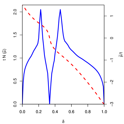
Figure 1: (Color online) Density of electronic states at the Fermi energy $t\,N(\widetilde{\mu})$ (solid blue line, left axis) and the chemical potential $\widetilde{\mu}/t$ (dashed red line, right axis) vs doping $\delta$.

The DOS at the Fermi energy $N(\widetilde{\mu})$ and the chemical potential $\widetilde{\mu}$ for $-3\leq\widetilde{\mu}/t\leq 1.5$ at zero temperature are plotted in Fig. 1 for doping $0\leq\delta\leq 1$. The two peaks of the DOS correspond to the VHS in two bands. The DOS is nonsymmetric with respect to $\widetilde{\mu}=0$ in comparison with the DOS of graphene due to the renormalization of the hopping parameter in (64), where we use $\widetilde{t}=t\,Q=t\,(1+\delta)/2$ neglecting the electron and spin contributions in Eq. (34).

We note that there are misprints in Ref. Vladimirov18 , Eqs. (26) and (29) for the GFs, in comparison with Eqs. (62) and (63), where we have opposite signs. But the expressions for the correlation functions $n_{A\sigma}({\bf k})=\langle X_{{\bf k}A}^{\sigma 0}X_{{\bf k}A}^{0\sigma}\rangle$ and $\langle X_{{\bf k}B}^{\sigma 0}X_{{\bf k}A}^{0\sigma}\rangle$ in Ref. Vladimirov18 are correct.

III.3 Anomalous Green functions

To calculate the superconducting $T_{c}$ we use the linearized approximation for the anomalous GFs (50) and (51). They are determined by the relations:

$$F_{AA}^{\sigma}({\bf k},\omega)=\frac{Q\,A_{31}^{\sigma}({\bf k},\omega)}{[\omega^{2}-\varepsilon^{2}_{+}({\bf k})][\omega^{2}-\varepsilon^{2}_{-}({\bf k})]},$$ (65)

$$A_{31}^{\sigma}({\bf k},\omega)=-\Delta_{AB\sigma}(-{\bf k})\,(\omega-\widetilde{\mu})\,\widetilde{t}\,\gamma({\bf k})$$

$$+\Delta_{AB\sigma}({\bf k})(\omega+\widetilde{\mu})\,\widetilde{t}\,\gamma^{*}({\bf k})$$

$$+\Delta_{\sigma}\,(\omega^{2}-\widetilde{\mu}^{2}-\widetilde{t}^{2}\,|\gamma({\bf k})|^{2}),$$ (66)

$$F_{AB}^{\sigma}({\bf k},\omega)=\frac{Q\,A_{41}^{\sigma}({\bf k},\omega)}{[\omega^{2}-\varepsilon^{2}_{+}({\bf k})][\omega^{2}-\varepsilon^{2}_{-}({\bf k})]},$$ (67)

$$A_{41}^{\sigma}({\bf k},\omega)=\Delta_{AB\sigma}({\bf k})(\omega^{2}-\widetilde{\mu}^{2})$$

$$-\Delta_{AB\sigma}(-{\bf k})\,\widetilde{t}^{2}\,\gamma^{2}({\bf k})+\Delta_{\sigma}\,2\widetilde{\mu}\,\widetilde{t}\,\gamma({\bf k}).$$ (68)

The corresponding anomalous correlation function $\,F_{BA}^{{\sigma}}({\bf k})=\langle X^{0\bar{\sigma}}_{-{\bf k}B}X^{0\sigma}_{{\bf k}A}\rangle\,$ in the gap equations (III.1), (III.1) determined by the GF (67) is given by

$$F_{BA}^{{\sigma}}({\bf k})=-\frac{1}{\pi}\int_{-\infty}^{\infty}\frac{d\omega}{\exp(\omega/T)+1}\;{\rm Im}F_{AB}^{\sigma}({\bf k},\omega)$$ (69)

$$= \frac{Q\,}{\varepsilon^{2}_{-}({\bf k})-\varepsilon^{2}_{+}({\bf k})}\Bigl{\{}\frac{A^{\sigma}_{41}(\omega=\varepsilon_{+}({\bf k}))}{2\varepsilon_{+}({\bf k})}\tanh\frac{\varepsilon_{+}({\bf k})}{2T}$$

$$- \frac{A^{\sigma}_{41}(\omega=\varepsilon_{-}({\bf k}))}{2\varepsilon_{-}({\bf k})}\tanh\frac{\varepsilon_{-}({\bf k})}{2T}\Bigr{\}}.$$

IV Gap equations and $\bf T_{c}$

Let us consider solutions for the gaps of different symmetries. In particular, the extended $s$-wave gap (III.1) determined by the bond-independent anomalous correlation function (69) can be written as:

$$\Delta_{AB\sigma}({\bf k})=\Delta_{AB\sigma}\,\sum_{{\alpha}}\exp[i{\bf(k\delta_{\alpha}}]=\Delta_{AB\sigma}\,\gamma({\bf k}).$$ (70)

The $d+id^{\prime}$-wave pairing is determined by the gap which has different phases on bonds (Refs. Black07 ; Jiang08 ; Gu13 ):

$$\Delta_{AB\sigma}({\bf k})=\sum_{\alpha}\Delta^{\alpha}_{\sigma}\exp[i{\bf k\delta_{\alpha}}],\;\Delta^{\alpha}_{\sigma}=\Delta_{1\sigma}e^{i(2\pi/3)\alpha}.$$ (71)

The numerical solution of the gap equations yields $T_{c}$ as a function of doping given below, where we use the renormalized hopping parameter $\widetilde{t}=t\,(1+\delta)/2$ (see Sect. III.2). Note that in our mean-field approach in two dimensions, $T_{c}$ is the temperature of Cooper-pair formation without superconducting long-range order (see, e.g., Refs. Kotov12 ; Uchoa07 ).

It should be pointed out that for the conventional Fermi-liquid we can have the $s$-wave pairing on a single site given by the anomalous correlation function $\langle a_{i\bar{\sigma}}a_{i\sigma}\rangle$. In terms of HOs this pairing can be described by the equation:

$$\langle a_{i\bar{\sigma}}a_{i\sigma}\rangle=\langle X_{i}^{02}\rangle=\langle X_{i}^{0\bar{\sigma}}X_{i}^{\bar{\sigma}2}\rangle\neq 0,$$ (72)

which shows that the double occupancy of one lattice site is permitted but in the two Hubbard subbands. For the Hubbard model in the limit of strong correlations, i.e., for the $t$-$J$ model, this pairing is prohibited due to the no-double-occupancy restriction which in terms of HOs, as was proposed in Ref. Plakida89 , can be written as:

$$\langle X_{i}^{0\bar{\sigma}}X_{i}^{0\sigma}\rangle=\langle a_{i\bar{\sigma}}(1-n_{i,{\sigma}})\,a_{i\sigma}(1-n_{i,\bar{\sigma}})\rangle\equiv 0.$$ (73)

As shown in Sect. IV.4, both the ${\bf k}$-independent $s$-wave pairing with the gap (III.1) and the extended $s$-wave pairing with the gap (70) violate this condition and must be excluded from a rigorous point of view. For the $d$-pairing with the gap (71) the condition (73) is fulfilled.

However, in several publications this constraint has not been rigorously taken into account, for example using the phenomenological $t$-$J$ model (see Ref. Black07 where the double-site occupancy is included in the Hilbert space), or introducing the statistical weighting factors $g_{t}=2\delta/(1+\delta)$ and $g_{J}=4/(1+\delta)^{2}$ in the $t$-$J$ model (see, Refs. Black14 ; Wu13 ), as discussed in Sect. I, or using the Gutzwiller projector $P_{g}=\prod_{i}(1-g\,n_{i\uparrow}n_{i\downarrow})$ with $\,g<1\,$ treated as variational parameter (see, e.g., Ref. Pathak10 ). To compare our results with these studies we have considered the ${\bf k}$-independent $s$-wave pairing in Sect. IV.1 and the extended $s$-wave pairing in Sect. IV.2.

IV.1 ${\bf k}$-independent $s$-wave gap equation

For the ${\bf k}$-independent $s$-wave gap (III.1) we have

$$\Delta_{\sigma} = \frac{2t}{Q}\sum_{l}\,\langle X_{lB}^{0\bar{\sigma}}X_{iA}^{0\sigma}\rangle$$ (74)

$$= \frac{2t}{QN}\sum_{{\alpha}}\sum_{\bf q}\exp[-i{\bf q\delta_{\alpha}}]\,F_{BA}^{\sigma}({\bf q}).$$

Assuming that $t\gg J$ we can solve the equation for $\Delta_{\sigma}$ considering the ${\bf q}$-dependent part of the gap $\Delta_{AB\sigma}({\bf q})$ in $A^{\sigma}_{41}(\omega,{\bf q})$ (68) as a small perturbation. We obtain the gap equation:

$$\Delta_{\sigma} = \frac{\Delta_{\sigma}\,t}{N}\,\sum_{\bf q}|\gamma({\bf q})|\Bigl{[}\frac{1}{2\varepsilon_{+}({\bf q})}\tanh\frac{\varepsilon_{+}({\bf q})}{2T_{c}}$$ (75)

$$- \frac{1}{2\varepsilon_{-}({\bf q})}\tanh\frac{\varepsilon_{-}({\bf q})}{2T_{c}}\Bigr{]}\Bigr{\}}.$$

We find a solution for $T_{c}$ only for hole doping $\delta\leq 0.32$ when $\tilde{\mu}>0$. It has a high maximum value, $T_{c}\sim 0.25t$, due to the strong pairing interaction $t\gg J$. Note that the coupling proportional to the hopping parameter $t$ is due to the kinematical interaction induced by the commutation relations (4) for the HOs. The same type of pairing occurs in the $t$–$J$ model on the square lattice (see Ref. Plakida89 ) which has been disregarded, since it violates the constraint of no-double-occupancy (73). As shown in Sect. IV.4, the $s$-wave pairing described by the ${\bf k}$-independent gap $\Delta_{\sigma}$ (74) on the honeycomb lattice also violates the constraint (73), and in what follows we take the solution $\Delta_{\sigma}=0$.

IV.2 Extended $s$-wave gap equation

Using Eq. (69) the gap equation (III.1) reads

$$\Delta_{AB\sigma}({\bf k})=\frac{J}{2N}\sum_{\bf q}\sum_{{\alpha}}\exp[i{\bf(k-q)\delta_{\alpha}}]\Delta_{AB\sigma}({\bf q})$$ (76)

$$\times \Bigl{[}\frac{1}{2\varepsilon_{+}({\bf q})}\tanh\frac{\varepsilon_{+}({\bf q})}{2T_{c}}+\frac{1}{2\varepsilon_{-}({\bf q})}\tanh\frac{\varepsilon_{-}({\bf q})}{2T_{c}}\Bigr{]}$$

$$- \frac{J}{N}\sum_{\bf q}\sum_{\alpha}\exp[i{\bf(k-q)\delta_{\alpha}}]\frac{\widetilde{t}^{2}}{4\tilde{\mu}\,\tilde{t}|\gamma({\bf q})|}$$

$$\times\Bigl{[}\Delta_{AB\sigma}({\bf q})|\gamma({\bf q})|^{2}-\Delta_{AB\sigma}(-{\bf q})\,\ \gamma^{2}({\bf q})\Bigr{]}$$

$$\times \Bigl{[}\frac{1}{2\varepsilon_{+}({\bf q})}\tanh\frac{\varepsilon_{+}({\bf q})}{2T_{c}}-\frac{1}{2\varepsilon_{-}({\bf q})}\tanh\frac{\varepsilon_{-}({\bf q})}{2T_{c}}\Bigr{]}.$$

Taking into account that the second term vanishes for the bond-independent gap $\Delta_{AB\sigma}({\bf k})=\Delta_{AB\sigma}\,\gamma({\bf k})$ because of $\,\gamma({\bf q})|\gamma({\bf q})|^{2}-\gamma^{*}({\bf q})\,\ \gamma^{2}({\bf q})=0\,$, we obtain the gap equation

$$\gamma({\bf k})=\frac{J}{2N}\sum_{\bf q}\sum_{\alpha}\exp[i{\bf(k-q)\delta_{\alpha}}]\gamma({\bf q})$$ (77)

$$\times \Bigl{[}\frac{1}{2\varepsilon_{+}({\bf q})}\tanh\frac{\varepsilon_{+}({\bf q})}{2T_{c}}+\frac{1}{2\varepsilon_{-}({\bf q})}\tanh\frac{\varepsilon_{-}({\bf q})}{2T_{c}}\Bigr{]}.$$

The solution of this equation shows that $T_{c}(\delta)$ linearly increases with doping and vanishes for large $\,\delta\,$ depending on $J$, e.g., $T_{c}(\delta)=0$ at $\delta>0.2$ for $J=t/2$. The maximum value of $T_{c}$ rapidly increases with the interaction $J$, e.g., $T_{c}^{\rm max}=0.035\,t\;(0.082\,t)\,$ for $J=t/3\;(\,t/2)$. Though the extended $s$-wave pairing also violates the constraint of no-double-occupancy (73), we consider it to compare our results with calculations for the $t$-$J$ model, where this restriction has not been rigorously taken into account.

IV.3 $d$-wave gap equation

In the case of $d$-wave symmetry ($d+id^{\prime}$) for the bond-dependent gap (71) we have the same equation (76). The direct numerical calculation for this gap reveals that the second term in the integral gives no contribution. It is convenient to consider the equation for a particular value of $\alpha$ for the phase sensitive contribution:

$$\Delta^{\alpha}_{\sigma}\exp[i{\bf(k\delta_{\alpha}}]=\Delta_{1\sigma}e^{i(2\pi/3)\alpha}\exp[i{\bf k\delta_{\alpha}}]$$ (78)

$$=\frac{J}{2N}\sum_{\bf q}\exp[i{\bf(k-q)\delta_{\alpha}}]\sum_{\beta}\,\Delta_{1\sigma}\,e^{i(2\pi/3)\beta}\exp[i{\bf q\delta_{\beta}}]$$

$$\times \Bigl{[}\frac{1}{2\varepsilon_{+}({\bf q})}\tanh\frac{\varepsilon_{+}({\bf q})}{2T_{c}}+\frac{1}{2\varepsilon_{-}({\bf q})}\tanh\frac{\varepsilon_{-}({\bf q})}{2T_{c}}\Bigr{]}.$$

Cancelling out the terms $\Delta_{1\sigma}\,\exp[i{\bf k\delta_{\alpha}}]$ we write this equation as

$$1=\frac{J}{2\,N}\sum_{\bf q}\sum_{\beta}\exp[i{\bf q}(\delta_{\beta}-\delta_{\alpha})]e^{i(2\pi/3)(\beta-\alpha)}$$

$$\times \Bigl{[}\frac{1}{2\varepsilon_{+}({\bf q})}\tanh\frac{\varepsilon_{+}({\bf q})}{2T_{c}}+\frac{1}{2\varepsilon_{-}({\bf q})}\tanh\frac{\varepsilon_{-}({\bf q})}{2T_{c}}\Bigr{]}.$$

Considering the vectors $a_{\beta\alpha}\equiv\delta_{\beta}-\delta_{\alpha}$ we can see that different values of $\beta-\alpha$ correspond to a set of three vectors, one is equal to zero, and the other two are the lattice vectors. The change of $\alpha$ rotates the whole set by $2\pi/3$ due to the $C_{3}$ symmetry of the lattice so that the above equation does not depend on $\alpha$. Therefore, all three equations for various $\alpha$ are the same. The equation for $\alpha=0$ reads:

$$1=\frac{J}{N}\sum_{\bf q}\frac{1}{2}\sum_{\beta}\exp[i{({\bf q}({\bf\delta}_{\beta}-{\bf\delta}_{0})}]e^{i(2\pi/3)\beta}$$

$$\times \Bigl{[}\frac{1}{2\varepsilon_{+}({\bf q})}\tanh\frac{\varepsilon_{+}({\bf q})}{2T_{c}}+\frac{1}{2\varepsilon_{-}({\bf q})}\tanh\frac{\varepsilon_{-}({\bf q})}{2T_{c}}\Bigr{]}.$$

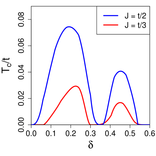
Figure 2: (Color online) $T_{c}(\delta)$ for the $d$-wave pairing with $J=t/3$ (dotted curve) and $J=t/2$ (bold line).

This equation was solved numerically for various values of $J/t$. The results for $T_{c}$ as a function of the hole doping $\delta$ are depicted in Fig. 2 and Fig. 3. $T_{c}(\delta)$ has a two-peak structure with the maxima corresponding to the VHS in the DOS shown in Fig. 1.

The transition temperature $T_{c}$ rapidly increases with the interaction $J/t$ in Eq. (LABEL:g32c), as was also found in Ref. Black07 . For small $J/t=1/3$ in Fig. 2 we get a smooth increase of $T_{c}$ with $\delta$ and $T_{c}=0$ (or exponentially small) for $\delta<0.05$ similar to the $d$-wave pairing in the one-band $t$–$J$ model on the square lattice (see Ref. Plakida99 ). In Ref. Gu13 for $J/t=1/3$ the superconducting order at $T=0$ was found for $0<\delta<0.4$, but in Ref. Black07 $T_{c}$ is exponentially small for $\delta<0.05$ when $J=0.8\,t$.

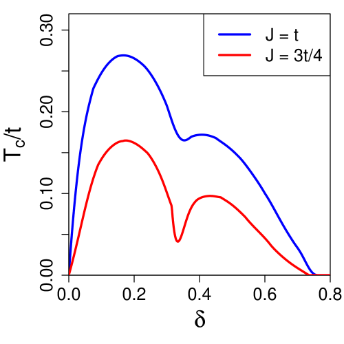
Figure 3: (Color online) $T_{c}(\delta)$ for the $d$-wave pairing with $J=3t/4$ (dotted curve) and $J=t$ (bold line).

For $J=3\,t/4$ in Fig. 3 the maximum of $T_{c}\approx 0.15t$ is comparable with the maximum value of $T_{c}\approx 0.1t$ in Ref. Black14 for $J/t=0.8$ and larger than $T_{c}\approx 0.05t$ in Ref. Black07 for $J/t=0.8$. As was claimed in these publications, such values of $T_{c}$ with the hopping parameter $t\approx 2.5$ eV in graphene would result in a room high-$T_{c}$ SC of electrons on the honeycomb lattice at optimal doping. The variational Monte Carlo calculation for the RVB theory in Ref.  Pathak10 shows that $T_{c}$ can be estimated as about twice of the room temperature. For small values of $J<J_{c}=0.75\,t\,$ there is no pairing at half-filling for $\tilde{\mu}=0$. For large values of $J/t$ a sharp increase of $T_{c}$ with $\delta$ is found in Fig. 3, and for $J>J_{c}$ $T_{c}$ is nonzero at $\tilde{\mu}=0$. In this region we can observe the gapless SC, as was also found in Ref. Uchoa07 for the $s$-wave pairing in graphene for the nn BCS coupling parameter $g_{1}>g_{1}^{c}$.

Taking into account the results of Ref. Vladimirov18 for the $t$–$J$ model on the honeycomb lattice, where AF long-range order at $T=0$ was observed for $\delta\lesssim 0.1$, we argue that the AF and superconducting ground-state order may coexist in the range $\delta\lesssim 0.1$, in agreement with the numerical calculations in Ref. Gu13 .

Let us compare the results for the extended $s$-wave pairing and $d$-wave pairing. As was found in Sect. IV.2, the maximum value of $T_{c}^{\rm max}\approx 0.082\,t\,$ for $J=t/2$ is nearly the same as in the case of $d$-wave pairing in Fig. 2. It contradicts to the results of Ref. Black07 , where $T_{c}$ for the $d$-wave pairing is much larger than for the extended $s$-wave pairing. Note that in Ref. Black07 the mean-field RVB theory was used, where the restriction of no-double-occupancy has not been taken into account. On the other hand, in Refs. Black14 ; Wu13 , where the renormalized mean-field approximation determined by the parameters $g_{t}$ and $g_{J}$ for the $t$–$J$ model was employed, the maximum value of the order parameter (and $T_{c}$) for the extended $s$-wave pairing and the $d$-wave pairing are quite close. So we can say that accounting for strong correlations both in our approach and in the renormalized mean-field approximation results in close maximum values of $T_{c}$ for the extended $s$-wave and $d$-wave pairing. However, it should be stressed that the constraint (73) excludes the $s$-wave pairing. This conclusion is supported by the calculations for the $t$–$J$ model in Ref. Gu13 , where the projected character of the electron operators has been implemented and only $d$-wave pairing has been found.

IV.4 Constraint for the s-wave pairing

Let us consider the restriction of no-double-occupancy (73) for the Hubbard operators:

$$\langle X_{iA}^{0\bar{\sigma}}X_{iA}^{0\sigma}\rangle=0.$$ (81)

Using the GF $F_{AA}^{\sigma}({\bf k},\omega)$ (65) this condition reads

$$\langle X_{iA}^{0\bar{\sigma}}X_{iA}^{0\sigma}\rangle=\frac{1}{N}\,\sum_{\bf k}\int_{-\infty}^{\infty}\frac{d\omega}{\exp(\omega/T)+1}$$

$$\times[-\frac{1}{\pi}]\,{\rm Im}\frac{Q\,A_{31}({\bf k},\omega)}{[\omega^{2}-\varepsilon^{2}_{+}({\bf k})][\omega^{2}-\varepsilon^{2}_{-}({\bf k})]}=0.$$ (82)

where the function $A_{31\sigma}({\bf k},\omega)$ is given by (66). This condition for the $s$-wave pairing determined by the gap function $\Delta_{\sigma}$ (III.1), where $A_{31\sigma}(\omega=\varepsilon_{\pm}({\bf k}))=\mp 2\Delta_{\sigma}\,\widetilde{\mu}\widetilde{t}\,|\gamma({\bf k})|$, results in the relation:

$$\langle X_{iA}^{0\bar{\sigma}}X_{iA}^{0\sigma}\rangle = -\frac{Q\,\Delta_{\sigma}}{2N}\,\sum_{\bf k}\Bigl{[}\frac{1}{2\varepsilon_{+}({\bf k})}\tanh\frac{\varepsilon_{+}({\bf k})}{2T}$$ (83)

$$+\frac{1}{2\varepsilon_{-}({\bf k})}\tanh\frac{\varepsilon_{-}({\bf k})}{2T}\Bigr{]}.$$

The summation over ${\bf k}$ does not vanish for a positively defined integrand. Therefore, the $s$-wave pairing with the ${\bf k}$-independent gap $\Delta_{\sigma}$ violates the kinematic restriction (82) and is ruled out.

For the extended $s$-wave pairing with the gap (70) we have $A_{31\sigma}(\omega=\varepsilon_{\pm}({\bf k}))=2\Delta_{AB\sigma}\,\widetilde{\mu}\,\widetilde{t}\,|\gamma({\bf k})|^{2}$, and the relation (82) reads:

$$\langle X_{iA}^{0\bar{\sigma}}X_{iA}^{0\sigma}\rangle = -\frac{Q\,\Delta_{AB\sigma}}{2N}\,\sum_{\bf k}|\gamma({\bf k})|\Bigl{[}\frac{1}{2\varepsilon_{+}({\bf k})}\tanh\frac{\varepsilon_{+}({\bf k})}{2T}$$ (84)

$$-\frac{1}{2\varepsilon_{-}({\bf k})}\tanh\frac{\varepsilon_{-}({\bf k})}{2T}\Bigr{]}.$$

The summation over ${\bf k}$ does not vanish except for $\widetilde{\mu}=0$ when $\varepsilon_{+}({\bf k})=-\varepsilon_{-}({\bf k})$. For other doping the correlation function (84) is non-zero that violates the kinematic restriction (82), and the extended $s$-wave pairing cannot be realized.

Finally, let us consider the $d$-wave pairing with the bond-dependent gap (71). In this case, for the function (66) we have

$$A_{31}(\omega=\varepsilon_{\pm}({\bf k}))=2\widetilde{\mu}\,\widetilde{t}\,\gamma({\bf k})\sum_{\alpha}\Delta^{\alpha}_{\sigma}\exp[-i{\bf k\delta_{\alpha}}]$$

$$\pm\widetilde{t}^{2}\,|\gamma({\bf k})|\,\sum_{\alpha}\Delta^{\alpha}_{\sigma}\,2i{\rm Im}[\gamma^{*}({\bf k})\exp(i{\bf k\delta_{\alpha}})],$$ (85)

where the relation $\,\gamma^{*}({\bf k})\exp(i{\bf k\delta_{\alpha}})-\gamma({\bf k})\exp(-i{\bf k\delta_{\alpha}})=2i\,{\rm Im}(\gamma^{*}({\bf k})\exp(i{\bf k\delta_{\alpha}}))$ was used. For the correlation function (82) we obtain:

$$\langle X_{iA}^{0{\sigma}}X_{iA}^{0\bar{\sigma}}\rangle=\frac{Q}{2N}\,\sum_{\alpha}\Delta^{\alpha}_{\sigma}\sum_{\bf k}\frac{\gamma({\bf k})}{|\gamma({\bf k})|}\exp(-i{\bf k}\delta_{\alpha})$$ (86)

$$\times \Big{[}\frac{1}{2\varepsilon_{+}({\bf k})}\tanh\frac{\varepsilon_{+}({\bf k})}{2T}-\frac{1}{2\varepsilon_{-}({\bf k})}\tanh\frac{\varepsilon_{-}({\bf k})}{2T}\Big{]}$$

$$+ \frac{Q\,\widetilde{t}}{4\widetilde{\mu}}\,\frac{1}{N}\,\sum_{\bf k}\ \sum_{\alpha}\Delta^{\alpha}_{\sigma}\,2i\,{\rm Im}[\gamma^{*}({\bf k})\exp(i{\bf k\delta_{\alpha}})]$$

$$\times \Big{[}\frac{1}{2\varepsilon_{+}({\bf k})}\tanh\frac{\varepsilon_{+}({\bf k})}{2T}+\frac{1}{2\varepsilon_{-}({\bf k})}\tanh\frac{\varepsilon_{-}({\bf k})}{2T}\Big{]}.$$

In the first term the summation over ${\bf k}$ does not depend on $\alpha$ due to the $C_{3}$ symmetry of $\gamma({\bf k})$ and $\varepsilon_{\pm}({\bf k})$. Therefore, the summation over $\alpha$ of the gap function $\Delta^{\alpha}_{\sigma}$ can be done independently that results in the vanishing of the first term: $\sum_{\alpha}\Delta^{\alpha}_{\sigma}=\Delta_{1\sigma}\sum_{\alpha}\exp(i(2\pi/3)\alpha)=0$. The second term also gives no contribution due to summation over ${\bf k}$ of the odd in ${\bf k}$ function ${\rm Im}[\gamma^{*}({\bf k})\exp(i{\bf k\delta_{\alpha}})]=i\sum_{\beta}\sin[{\bf k}(\delta_{\alpha}-\delta_{\beta})]$. So, the $d$-wave pairing with the gap (71) does not violate the condition of no-double-occupancy (82). This conclusion was checked by the direct integration over ${\bf k}$ in Eq. (86).

V Conclusion

In this paper a microscopic theory of superconductivity in electronic systems with strong correlations is presented within the $t$–$J$ model on the honeycomb lattice. The constraint of no-double-occupancy in the two-band $t$–$J$ model is rigorously taken into account by employing the HO technique. The superconducting $T_{c}$ as a function of doping is calculated for the $d+id^{\prime}$ gap function. It reveals a two-peak structure related to the two VHS in the two-band electronic spectrum. For large values of $J>J_{c}=0.75t$ a gapless superconductivity is found at $\tilde{\mu}=0$. It is suggested that for small doping, $\delta\lesssim 0.1$, the AF long-range order found in Vladimirov18 may coexist with the $d+id^{\prime}$ superconductivity.

We have also calculated $T_{c}$ for the extended $s$-wave pairing to compare it with the results obtained for the $t$–$J$ model, where the constraint has been neglected or considered approximately. In the latter case the results for the maximum value of $T_{c}$ are comparable. However, we have shown that the $s$-wave pairing violates the constraint and should be ruled out.

In graphene with the large hopping parameter $t\approx 2.5$ eV the single-site Coulomb repulsion is not strong enough, $U/t=4-5$ Neto09 . Therefore, the application of the $t$–$J$ model to graphene is questionable. In our theory we have the renormalized hopping parameter $\tilde{t}$ (34) which is small in the region $\delta\leq 0.4$, where the nn correlation function $\,C_{1}\leq-0.1$ Vladimirov18 . Therefore, we have $U/\tilde{t}\gg 1$, and the application of the $t$–$J$ model can be justified. Moreover, complicated structures like sulfur-graphite composites Black07 may result in a larger value of $U/t$, and high-$T_{c}$ superconductivity can be achieved.

- (1) A. H. Castro Neto, F. Guinea, N. M. R. Peres, K. S. Novoselov, A. K. Geim, Rev. Mod. Phys. 81, 109 (2009)
- (2) V. N. Kotov, B. Uchoa, V. M. Pereira, F. Guinea, A. H. Castro Neto, Rev. Mod. Phys. 84, 1067 (2012)
- (3) A. M. Black-Schaffer, Wei Wu, K. Le Hur, Phys. Rev. B 90, 054521 (2014)
- (4) B. Uchoa, G. G. Cabrera, A. H. Castro Neto, Phys. Rev. Lett. 71, 184509 (2005)
- (5) B. Uchoa, A. H. Castro Neto, Phys. Rev. Lett. 98, 146801 (2007)
- (6) J. Hubbard, Proc. Roy. Soc. (London) A 276, 238 (1963)
- (7) C. Honerkamp, Phys. Rev. Lett. 100, 146404 (2008)
- (8) J. P. L. Faye, P. Sahebsara, D. Sènèchal, Phys. Rev. B 92, 085121 (2015)
- (9) A. M. Black-Schaffer, S. Doniach, Phys. Rev. B 75, 134512 (2007)
- (10) G. Baskaran, Phys. Rev. B 65, 212505 (2002)
- (11) Y. Jiang, Dao-Xin Yao, E. W. Carlson, Han-Dong Chen, Jiang Ping Hu, Phys. Rev. B 77, 235420 (2008)
- (12) S. Pathak, V. B. Shenoy, G. Baskaran, Phys. Rev. B 81, 085431 (2010)
- (13) Wei Wu, M. M. Scherer, C. Honerkamp, K. Le Hur, Phys. Rev. B 87, 094521 (2013)
- (14) S. Jiang, A. Mesaros, Y. Ran, Phys. Rev. X 4, 031040 (2014)
- (15) Z.-C. Gu, H.-C. Jiang, D. N. Sheng, H. Yao, L. Balents, X.-G. Wen, Phys. Rev. B 88, 155112 (2013)
- (16) Z.-C. Gu, H.-C. Jiang, G. Baskaran, arXiv:1408.6820
- (17) R.S. Markiewicz, J. Phys. Chem. Solids 58, 1179 (1997)
- (18) J. L. McChesney, A. Bostwick, T. Ohta, T. Seyller, K. Horn, J. Gonza´lez, E.Rotenberg, Phys. Rev. Lett. 104, 136803 (2010)
- (19) D. J. Scalapino, E. Loh, J. E. Hirsch, Phys. Rev. B 35, 6694 (1987)
- (20) J. González, Phys. Rev. B 78, 205431 (2008)
- (21) T. Ma, F. Yang, H. Yao, Hai-Qing Lin, Phys. Rev. B 90, 245114 (2014)
- (22) R. Nandkishore, A. V. Chubukov, Phys. Rev. B 86, 115426 (2012)
- (23) X.-Y. Xu, S. Wessel, Z.-Y. Meng, Phys. Rev. B 94, 115105 (2016)
- (24) F.-C. Zhang, C. Gros, T. M. Rice, H. Shiba, Supercond. Sci. Technol. 1, 36 (1988)
- (25) G. Martinez, P. Horsch Phys. Rev. B 44, 317 (1991)
- (26) Anderson P.W., Science 235, 1196 (1987)
- (27) J. Hubbard, Proc. Roy. Soc. A (London) 285, 542 (1965)
- (28) A. A. Vladimirov, D. Ihle, N. M. Plakida, Eur. Phys. J. B 91, 195 (2018)
- (29) H. Mori, Prog. Theor. Phys. 34, 399 (1965)
- (30) D. N. Zubarev, Usp. Phys. Nauk 71, 71 (1960) [translated in Sov. Phys. Usp. 3, 320 (1960)], Nonequilibrium Statistical Thermodynamics, Consultants Bureau, New-York, 1974.
- (31) Plakida N. M., In: Theoretical Methods for Strongly Correlated Systems, Chap. 6, pp. 173–202. Eds. A. Avella and F. Mancini, Springer Series in Solid–State Sciences Vol. 171, Springer, Heidelberg, 2011.
- (32) N.M. Plakida, V.S. Oudovenko, Phys. Rev. B 59, 11949 (1999)
- (33) N.M. Plakida, V.S. Oudovenko, Eur. Phys. J. B 86, 115 (2013)
- (34) N.M. Plakida, V. Yushankhai, I.V. Stasyuk, Physica C 160, 80 (1989)