Tagged particle dynamics in one dimensional $A+A\to kA$ models with the particles biased to diffuse towards their nearest neighbour

Abstract

Dynamical features of tagged particles are studied in a one dimensional $A+A\rightarrow kA$ system for $k=0$ and 1, where the particles $A$ have a bias $\epsilon$ $(0\leq\epsilon\leq 0.5)$ to hop one step in the direction of their nearest neighboring particle. $\epsilon=0$ represents purely diffusive motion and $\epsilon=0.5$ represents purely deterministic motion of the particles. We show that for any $\epsilon$, there is a time scale $t^{*}$ which demarcates the dynamics of the particles. Below $t^{*}$, the dynamics are governed by the annihilation of the particles, and the particle motions are highly correlated, while for $t\gg t^{*}$, the particles move as independent biased walkers. $t^{*}$ diverges as $(\epsilon_{c}-\epsilon)^{-\gamma}$, where $\gamma=1$ and $\epsilon_{c}=0.5$. $\epsilon_{c}$ is a critical point of the dynamics. At $\epsilon_{c}$, the probability $S(t)$, that a walker changes direction of its path at time $t$, decays as $S(t)\sim t^{-1}$ and the distribution $D(\tau)$ of the time interval $\tau$ between consecutive changes in the direction of a typical walker decays with a power law as $D(\tau)\sim\tau^{-2}$.

I Introduction

Reaction diffusion systems in their simplest form with diffusion and annihilation of particles have been studied over the years privman ; ligget ; krapivsky ; odor . These are nonequilibrium systems of diffusing particles undergoing certain reactions. Depending on the nature of the problem, the particles could be molecules, chemical or biological entities, opinions in societies or market commodities. Such systems are frequently used to describe various aspects of wide varieties of chemical, biological and physical problems. In the lattice version of the single species problem, the lattice is filled with particles (say $A$) with some probability initially and at each time step, the particles are allowed to jump to one of the nearest neighbouring sites (diffusion) with a certain probability. The simplest form of particle reaction is when a certain number $l$ of the particles meet: $lA\rightarrow kA$ with $k<l$. It is well known that annihilating random walkers with $l=2$ and $k=0$ corresponds to the Ising-Glauber kinetics while the coalescing case with $l=2$ and $k=1$ describes the dynamics of the $q$ state Potts model with $q\to\infty$, both at zero temperature and in one dimension derrida_95 . Such systems have been studied in one dimension racz ; amar ; avraham ; alcaraz ; krebs ; santos ; schutz ; oliveira as well as in higher dimensions kang ; peliti ; zumofen ; droz . Depending on the initial condition, whether one starts with even or odd number of particles, the steady state will contain no particles or one particle respectively. The focus in all these analysis is how the system approaches the steady state. In particular, one intends to know how the number of particles decays with time and the distribution of the intervals between the particles evolves with time.

Various reaction diffusion systems have been studied with different values of $k$ and $l$ in the past for different dynamical processes like ballistic annihilationkrap_ballistic ; bennaim ; krap_ballisticanni_2001 , Levy walks albano_levy ; krap_bennaim2016 and of course simple diffusion. However, what happens if the dynamical process is intrinsically stochastic and diffusive is an important question which has not been studied much. The idea behind all these studies is to find any universal behaviour in these system and the key factors which determine the universality. Here we ask the same question by introducing a bias which does not alter the existing features like conservation, range and nature of the interaction or the diffusional dynamics in the model.

We have studied the model $A+A\to kA$ where the particle $A$ diffuses with a preference towards its nearest neighbour. Both the annihilating case ($k=0$) and the coalescing case ($k=1$) have been considered. It is important to note that this bias does not affect the annihilation process and retains the Markovian property of the dynamics. This simple extension, indeed, leads to drastic changes in the bulk dynamical features. For $k=0$, the fraction of walkers $\rho(t)$ at time $t$ was found to decay as $\rho(t)\sim t^{-\alpha}$, where $\alpha\approx 1$ when the bias, however small, is introduced soham_ray_ps2011 ; ray_ps2015 . In the absence of the bias, it is known that $\alpha=1/2$. The value of $\alpha$ suggests that in the presence of the bias, the walkers, in the long time limit, behave as ballistic walkers.For the coalescing case with bias, the bulk behaviour is identical, i.e., $\alpha\approx 1$ (reported in the present paper).

The model considered in soham_ray_ps2011 ; ray_ps2015 may thus appear to be equivalent to the system of annihilating ballistic walkers at large times. But several features (e.g., persistence, domain growth etc.) of the dynamics show that it is actually not the same. Hence, to get a better understanding we study the dynamics of a tracer walker in the biased case for both ($k=0$ and $1$), specifically to check whether they perform ballistic motion or not.

In the following we briefly introduce the models and mention the different features studied and also the main results obtained. We have a bunch of walkers on a one dimensional ring. At every time step, the walker hops one step to its left or right with a bias $\epsilon$ to move in the direction of its nearest neighbour. $\epsilon=0$ implies no bias so that the walkers are purely random walkers and $\epsilon=\epsilon_{c}=0.5$ implies full bias so that the walker always moves towards its nearest neighbour. Except for this point, the motion is always stochastic.

For the annihilating case with $k=0$, we have a more detailed presentation of the results. First, the probability $P(x,t)$ that a particle is at a distance $x$ from its origin after time $t$ is estimated. We then calculate the probability that a walker changes its direction as a function of time. The distribution of the time intervals over which the walk continues in the same direction is also obtained. A change in the direction of motion can occur either due to diffusion or annihilation of the nearest particle(s). We find that the dynamics of the walkers are controlled by two time regimes. For time $t<t^{*}$, the dynamics are controlled by the annihilation of the particles. The motion of the walkers, in this regime, is highly correlated and the process is critical in the sense that there is no time scale in it. As a result, the probability $S(t)$ of the change in the direction of the motion of the walker at time $t$ decays with a power law; $S(t)\sim 1/t$. Similarly, the distribution $D(\tau)$ of the time interval $\tau$ spent between two changes in the direction of the motion of the walkers is scale free as $D(\tau)\sim 1/\tau^{2}$. We have found the full scaling behavior and arguments for the values of the exponents. The crossover time $t^{*}\sim(\epsilon_{c}-\epsilon)^{-1}$, so $\epsilon_{c}$ can be interpreted as a dynamical critical point where a diverging time scale exists.

We have also studied the coalescing model ($k=1$) with similar bias, i.e., $A+A\to A$ model. Without the bias, it is equivalent to the $A+A\to\emptyset$ model as far as the decay of particles in time is concerned. In presence of bias, the scaling of the fraction of surviving particles $\rho(t)\propto t^{-1}$ (details in section IV) shows that it is similar to the annihilating model. The dynamics of the particles are indeed different in the coalescing model as the distances between the particles are not much affected by a reaction, except for the surviving particle that remains after the reaction. Here we have focussed on the behaviour of $S(t)$ and $D(\tau)$ and find that the qualitative features of the dynamics of the tagged particle are again the same as in the $A+A\to\emptyset$ model. However, here the crossover to the diffusion behaviour occurs at later times, so that $t^{*}$ is higher in the $A+A\to A$ model. This is consistent with our inference that the early time regime is annihilation dominated as for $k=1$, the annihilation continues for a longer time.

II The Model, dynamics and simulation details

The model consists of walkers denoted by $A$, undergoing the reaction $A+A\to kA$. At each update, a site is selected randomly and if there is a particle on it, it moves towards its nearest neighbour with probability $\epsilon+0.5$ $(0\leq\epsilon\leq 0.5)$ and otherwise in the opposite direction. For $k=0$, if there is already another walker located on this neighbouring site, then both particles are annihilated and for $k=1$, one of them survives. Suppose, a walker is at site $i$ and its nearest neighbours are at $i+x$ and $i-y$ on its right and left respectively; the walker will hop one step towards right with probability $0.5+\epsilon$ and to left with probability $0.5-\epsilon$ if $x<y$. In the rare cases where the two neighbours are equidistant, the walker moves in either direction with equal probability.

When the bias $\epsilon=0.5$, the $k=0$ case corresponds to the spin model introduced in soham_ps2009 (see Appendix for details). Hence, the dynamical updating scheme used here for $k=0$ has a one to one correspondence with the original spin dynamics used in soham_ps2009 . As the spin system in soham_ps2009 was considered to be highly disordered initially, we start with a high density of walkers in this problem; specifically the number of walkers is chosen to be $L/2$ on a one dimensional lattice of size $L$. To maintain the correspondence with spin dynamics, the walkers are updated asynchronously and at each update a site is chosen randomly, rather than a walker, for updating. One Monte Carlo step (MCS) comprises of $L$ such updates. The same dynamical scheme was used in ray_ps2015 ; soham_ray_ps2011 where the bulk properties of the walker model were studied.

The dynamical scheme allows the possibility that a walker’s state may not be updated at all. This is because if a site is not selected, the position of the corresponding walker will not be updated. It may also happen that a walker is updated more than once in the following manner: if a walker moves to the site $j$ and the site $j$ is selected later, then the position of the same walker is updated again. This signifies that the net displacement of a particular walker may even be zero when it performs more than one movement in the same MCS. For all calculations, the final positions of the walkers after the completion of one MCS are considered. The results reported here are for simulations done on lattices of size 12000 or more and the maximum number of configuration studied was 2000. Periodic boundary condition has been used for all the simulations.

In the $A+A\to A$ model ($k=1$), the same dynamical scheme is used. Here, once two walkers meet, one of them will survive. In order to study the tagged particle dynamics, we need to label the surviving particle. We use the convention that the particle which makes the last movement survives. We have checked that the random convention (either of the two particles is taken to be the survivor randomly) leads to the same results qualitatively.

III Results for $A+A\to\emptyset$ $(k=0)$ model

To check the movement of individual walkers we took snapshots of the system at different times. Fig. 1(a) and (b) show the world lines of the motion of the particles for $\epsilon=0$ and $\epsilon=0.5$. It clearly shows that the motion of the individual particles in the two extreme cases are remarkably different. Annihilation dominates for $\epsilon=0.5$ while for $\epsilon=0$ the walk is diffusive as expected. For the intermediate values of $\epsilon$, both the mechanisms of diffusion and annihilation will be important and thus, as we will see later, give rise to the crossover effect for the system. To probe the dynamics of the particles, we have studied the following three quantities: (i) the probability distribution $P(x,t)$ of finding a particle $A$ at distance $x$ from its origin at time $t$, (ii) the probability $S(t)$ of the change in the direction in the motion of a walker at a time $t$ and (iii) the distribution $D(\tau)$ of the time interval $\tau$ between two successive changes in the direction of the motion of a walker. The results for each of these quantities are described in the following three subsections.

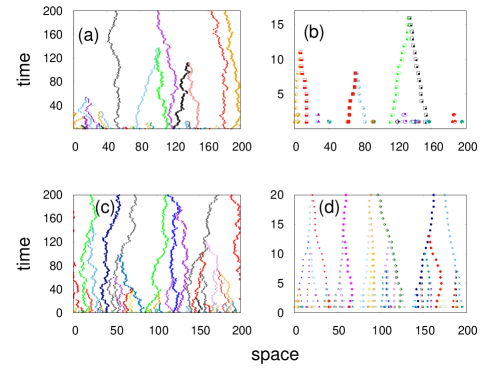
Figure 1: Snapshots of the system at different times for $\epsilon$=0 (a) and $\epsilon$=0.5 (b) for $A+A\to\emptyset$ model. Lower panel show the snapshots for $A+A\to A$ model for $\epsilon$=0 (c) and $\epsilon$=0.5 (d). The trajectories in different colors represent different particles.

III.1 Probability distribution $P(x,t)$

For $\epsilon=0$, the single particle motion is diffusive and the corresponding probability distribution $P(x,t)$ is known to be Gaussian. This remains true even in the presence of annihilation.

For $\epsilon\neq 0$, $P(x,t)$ changes drastically. The distributions are still symmetric as the motion of individual particles can occur in both directions (left and right). However, there is no peak at the origin ($x=0$) and instead a double peak structure emerges with a dip at $x=0$. To obtain a collapse of the data at different times, we note that the scaling variable is $x/\epsilon t$ for all values of $\epsilon$. We find that the collapsed data can be fit to the form

$$P(x,t)\epsilon t=f(\frac{x}{\epsilon t})\propto\exp[-\beta\{(\frac{\gamma x}{\epsilon t})^{2}-1\}^{2}].$$ (1)

The data collapse in the early time regime is shown in Fig. 2a. However, the data collapse as well as the above scaling form seems to be less accurate at later times. On investigating further, we find that while we attempt to fit the data individually for each $\epsilon$ and $t$ by the form given in Eq. (1), only in the early regime ($\epsilon t\lesssim 100$), both $\beta$ and $\gamma$ are constants. While $\gamma$ shows negligible dependence on $\epsilon$ and $t$, $\beta$ strongly depends on $\epsilon t$; beyond $\epsilon t=100$ it is no longer a constant but increases sharply as a function of $\epsilon t$. Hence the distribution scaled in the above manner shows a dip at the center which goes down with time while the peak heights increase such that the data do not collapse well as shown in Fig. 2b.

The above study suggests that at vary late stages, the scaled distribution will assume a double delta functional form and a universal scaling function exists only in the early time regime ($\epsilon t\lesssim 100$). We can relate the breakdown of the universal behaviour to the crossover phenomena that is revealed more clearly in the following subsections.

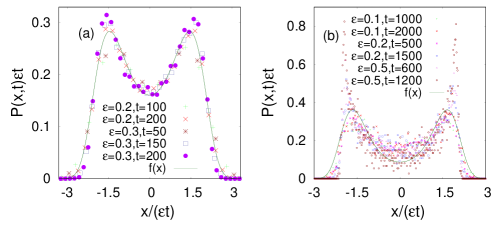
Figure 2: (a): Data collapse of ${P(x,t)\epsilon t}$ against ${x/\epsilon t}$ for $\epsilon=0.2$ and $0.3$ are shown at early time regime, (b): Data collapse of ${\it P(x,t)\epsilon t}$ against ${\it x/\epsilon t}$ are shown for $\epsilon=0.1,0.2,0.5$ at late time regime. These data are for the $A+A\to\emptyset$ model.

III.2 Probability of change in direction

The probability of direction change at time $t$ is obtained by estimating the fraction of walkers that change direction at time t. For $\epsilon=0$, as the system is diffusive, the probability of direction change $S(t)=p_{0}$, a constant independent of time. For a purely diffusive random walk, $p_{0}=0.5$. But here asynchronous dynamics have been used and this updating scheme allows the walkers to remain in the same state within a MCS as already discussed in the previous section. This dynamics can only decrease the probability of change in direction. $p_{0}$ for $\epsilon=0$ actually turns out to be $\approx 0.27$ numerically.

For $0<\epsilon<0.5$, the change in direction of a walker occurs due to two reasons; either due to the annihilation of a neighbouring walker or because of the diffusive component which is large for small $\epsilon$. At earlier times, the walker density is large and so the number of annihilation is considerable. Therefore the change in direction of the walkers is dominated by the annihilation process. However, as time progresses, annihilation becomes rarer and therefore the diffusive component becomes the dominating factor. So a saturation value $S_{sat}$ of $S(t)$ is reached at a later time, typically after a time $t^{*}$. The data for $S(t)$ is shown in Fig. 3 and the inset shows the variation of $S_{sat}$ with ${\epsilon_{c}-\epsilon}$ where $\epsilon_{c}=0.5$. As expected, $S_{sat}$ decreases as $\epsilon$ is made larger. In fact, we find that unless $\epsilon$ is very close $\epsilon_{c}$, the saturation is reached very fast, typically within one hundred MC step. $S_{sat}$ shows a linear variation with $\epsilon_{c}-\epsilon$, shown in inset of Fig. 3.

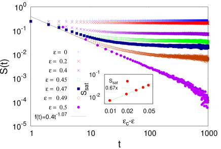
Figure 3: Probability of direction change of tagged particle for different $\epsilon$ in the $A+A\to\emptyset$ model. For $\epsilon=0.5$, it decays as $t^{-1}$. Inset shows the variation of $S_{sat}$ with $\epsilon_{c}-\epsilon$.

One can obtain a data collapse by plotting $S(t)t$ against $t(\epsilon_{c}-\epsilon)$, shown in Fig. 4. This indicates that one can write $S(t)$ as

$$S(t)=\frac{1}{t}g(z),$$ (2)

where $z=t(\epsilon_{c}-\epsilon)$ and $g(z)$ is a scaling function. $g(z)$ is constant for $z<1$ and $g(z)\sim z$ for large $z$. Therefore, $p_{\epsilon}\equiv S(t\to\infty)\propto(\epsilon_{c}-\epsilon)$, which is consistent with the variation of $S_{sat}$ with $(\epsilon_{c}-\epsilon)$ (see inset of Fig. 3). Hence one can argue that $t^{*}=(\epsilon_{c}-\epsilon)^{-1}$ acts as a timescale, below which $S(t)\propto t^{-\delta}$ with $\delta=1$. As $t^{*}$ diverges at $\epsilon_{c}$, there is no saturation region for $\epsilon=\epsilon_{c}$ and $S(t)$ shows a power law decay, $S(t)\sim t^{-1}$ for all times as shown in Fig. 3. The divergence of $t^{*}$ as $\epsilon\rightarrow\epsilon_{c}$ justifies that $\epsilon_{c}$ is the dynamical critical point.

One can argue that the value of $\delta$ is unity for the deterministic case $\epsilon=0.5$, where the walker always moves towards its nearer neighbour. A direction change can occur only if an adjacent walker is annihilated (however, this is a necessary but not sufficient condition). Let $A(t)$ be the number of annihilation taking place at time $t$. If $N(t)$ is the number of walkers at time $t$, $A(t)$ is given by $-\frac{dN}{dt}\propto t^{-\alpha-1}=t^{-2}$. Since $N(t)$ is proportional to $t^{-1}$ and $S(t)$ is proportional to $A(t)/N(t)$, therefore $S(t)\sim t^{-1}$. It may be added here that $A(t)$ and $N(t)$ have the same behaviour for all $\epsilon\neq 0$, however, for $\epsilon\neq 0.5$, direction change may occur even when there is no annihilation. The above argument is valid only for $\epsilon=0.5$ for which there is no diffusive component. However, the fact that $S(t)\propto t^{-1}$ in the early time regime for $\epsilon\neq 0.5$ also, shows that the annihilation plays the key role in the dynamics here; the diffusive component is virtually ineffective. Clearly a crossover behaviour occurs in time. The crossover occurs at a time when annihilation becomes rare. This depends on two factors: the density of the walkers and the strength of the bias. In time, the density decreases and beyond the crossover time $t^{*}$, the bias is not strong enough to cause two particles to come close enough and cause an annihilation. The motion effectively becomes uncorrelated. Obviously, the crossover occurs at later times as $\epsilon$, representing the bias, becomes larger and the inherent diffusive component becomes weaker making annihilations more probable. Therefore, at $\epsilon=0.5$, the fully biased point, $S(t)\propto t^{-1}$ and the crossover time diverges.

The nature of the walk remains ballistic in all regimes due to the bias, however small, to move towards the nearest neighbours. This is consistent with the conjecture that the probability distribution assumes a double delta form at large times mentioned in the last subsection.

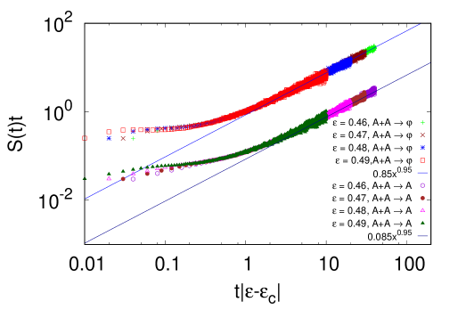
Figure 4: Variation of $S(t)t$ with $t|\epsilon-\epsilon_{c}|$ shows a data collapse for both the models $A+A\to\emptyset$ and $A+A\to A$, where $\epsilon_{c}=0.5$. Data for the $A+A\to A$ model have been shifted along $y$ axis for better clarity. The linear regions in the log-log plot are fitted to power law forms with the exponent very close to unity.

III.3 Distribution of time intervals between consecutive change in direction

Another interesting quantity is $D(\tau)$, the interval of time $\tau$ spent without change in direction of motion. For random walkers with $\epsilon=0$, the probability that in the time interval $\tau$, there is no direction change is given by

$$D(\tau)={p_{0}}^{2}({1-p_{0}})^{\tau}.$$ (3)

This reduces to an exponential form: $D(\tau)\propto\exp[-\tau\ln\{1/(1-p_{0})\}]$. Fig. 5a shows the data for $D(\tau)$ for $\epsilon=0$. From the numerical simulation, we find $D(\tau)\sim\exp(-\tau\ln 1.38)$ for $\epsilon=0$, which is consistent with $p_{0}\approx 0.27$.

For general values of $\epsilon\neq 0$, we note that $D(\tau)$ obeys the following form

$$D(\tau)\sim\frac{1}{\tau^{2}}\phi(z),$$ (4)

where $z=\tau(\epsilon_{c}-\epsilon)$ is the scaling argument and $\phi(z)$ is the scaling function. $\phi(z)$ is constant for $z<1$ and proportional to $\exp(-z)$ for $z\gg 1$. The data are shown in Fig. 5b.

Thus it is indicated that here also a crossover behaviour occurs at $\tau=\tau^{*}$ with $\tau^{*}\propto(\epsilon_{c}-\epsilon)^{-1}$, beyond which the exponential decay is observed and below which there will be a power law behaviour. Obviously for $\epsilon=0.5$, $\tau^{*}$ diverges such that only the power law decay will be observed with an exponent 2 which is indeed the case as shown in Fig. 5c.

It can be argued why the exponent is $2$ for $\epsilon=0.5$. Suppose the walker moves without direction change in the interval $t_{0}+1$ to $t_{0}+\tau$. This means it changes direction at times $t_{0}$ and $t_{0}+\tau+1$. Hence, $D(t_{0},\tau)$ is given by

$$D(t_{0},\tau) = S(t_{0})S(t_{0}+\tau+1)\prod_{x=1}^{\tau}[1-S(t_{0}+x)].$$

Using the variation of $S(t)\propto 1/t$ obtained in the last subsection,

$$D(t_{0},\tau) \propto (t_{0}^{-1})(t_{0}+\tau+1)^{-1}\prod_{x=1}^{\tau}(1-\frac{1}{t_{0}+x}).$$ (5)

Taking logarithm of both sides of Eq. (5) and converting summation into an integral, one gets

$$\ln D(t_{0},\tau) = -2\ln(t_{0}+\tau),$$

apart from a constant factor. One can always choose the origin $t_{0}$ to be zero, such that

$$D(\tau)\sim\tau^{-2}$$ (6)

showing consistency with the numerical results. (Fig. 5b).

One can also justify the crossover behaviour for $0<\epsilon<0.5$. Here, the crossover behaviour in $S(t)$ found in Sec. III.2, should be taken into account while calculating $D(\tau)$. $S(t)$ decays in a power law manner at short times to a constant value in the late time regime. The relatively larger value of $S(t)$ will be responsible for the behaviour of $D(\tau)$ for small $\tau$. Hence, for small $\tau$, the power law behaviour of $S(t)$ will be relevant for which it has been already shown that $D(\tau)\propto\tau^{-2}$. On the other hand, the constant (lower) value of $S(t)$ will be responsible for contribution to $D(\tau)$ for large values of $\tau$. For $t>t^{*}$, $S(t)=p_{\epsilon}=a_{0}(\epsilon_{c}-\epsilon)$, where $a_{0}$ is a constant less than unity (see Fig. 4). Using this value, one gets therefore $D(\tau)=(p_{\epsilon})^{2}(1-p_{\epsilon})^{\tau}\sim\exp(\tau\ln(1-a_{0}(\epsilon_{c}-\epsilon)))$. As $a_{0}(\epsilon_{c}-\epsilon)$ is less than unity, the expression for $D(\tau)$ simplifies to

$$D(\tau)\sim\exp(-a_{0}(\epsilon_{c}-\epsilon)\tau).$$ (7)

$D(\tau)$ can indeed be fit to an exponential form for large values of $\tau$ (see Fig. 5d): $D(\tau)\sim\exp(-b\tau)$ (as long as $\epsilon$ is not very close to $\epsilon_{c}$ for reasons that will be clarified later) and $b$ can be fitted to the form

$$b=b_{0}(\epsilon_{c}-\epsilon),$$ (8)

where $b_{0}=0.5$, shown in Fig. 6. This agrees with the expectation that $b$ should be varying linearly with $(\epsilon_{c}-\epsilon)$ as indicated by Eq. (7). It is also observed that $b$ approaches the value $\ln 1.38$ as $\epsilon\rightarrow 0$ and $b\rightarrow 0$ as $\epsilon\rightarrow\epsilon_{c}=0.5$ (Fig. 6).

Fig. 5b shows that for large values of the argument, beyond the crossover, the data collapse is not of very good quality. This is because as $\epsilon$ approaches 0.5 the crossover time increases and the exponential behaviour exists only for very large values of $\tau$ where the statistics is obviously poorer. This is the reason for which the estimation of $b$ for $\epsilon\rightarrow\epsilon_{c}$ becomes less reliable as mentioned before. On the other hand, to show the power law region one has to use values of $\epsilon$ fairly close to 0.5.

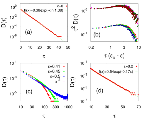
Figure 5: (a), (c) and (d) show data for the $A+A\to\emptyset$ model while (b) includes the data for the $A+A\to A$ model also. (a) Variation of $D(\tau)$ over $\tau$ for $\epsilon=0$ (b) Collapsed data for $D(\tau)\tau^{2}$ against $\tau(\epsilon_{c}-\epsilon)$ for $\epsilon=0.475,0.48,0.485$. Data for the $A+A\to A$ model (lower curves) have been shifted for better clarity. (c) shows the data for $D(\tau)$ against $\tau$ for $\epsilon=0.41,0.45,0.5$, where power law decay exists over a small time interval and power law region decreases with the decrease of $\epsilon$. (d) shows the variation of $D(\tau)$ against $\tau$ for $\epsilon=0.2$ and the data is fitted according to Eq. (4) for $\tau\gg t^{*}$ for $A+A\to\emptyset$ model.

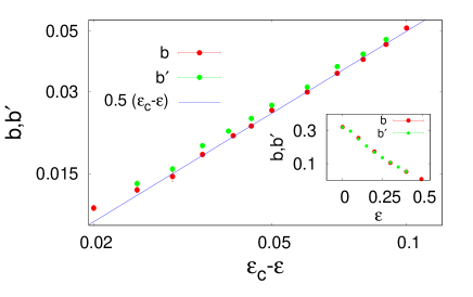
Figure 6: Variation of $b$ and $b^{\prime}$ with $\epsilon_{c}-\epsilon$ shown in a log-log plot when $\epsilon$ is very close to 0.5 and inset shows the variation with $\epsilon$ for the full range.

IV Results for $A+A\to A$ ($k=1$) model

For the $A+A\to A$ model, the $\epsilon=0$ case is known to have the scaling form for the fraction of surviving particles as $\rho(t)\propto t^{-1/2}$ krap_ballistic . In the biased case, with any $\epsilon\neq 0$ we find that the scaling is again like the $A+A\to 0$ case (with bias) as $\rho(t)\propto t^{-1}$ shown in Fig. 7. Typical snapshots of the walk are shown in Fig. 1(c) and (d).

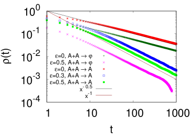
Figure 7: Variation of $\rho(t)$ with $t$ is shown in a log-log plot for different values of $\epsilon$ for $A+A\to\emptyset$ and $A+A\to A$ models.

For the motion of the tagged particles in the $A+A\to A$ model, we restrict the study to the probability of direction change and distribution of the time interval of motion executed without direction change. Again we find no significant change from the behaviour for the $A+A\to 0$ case., i.e., here also $S(t)\propto t^{-1}$ for $\epsilon=0.5$ while for other values of $\epsilon$, there is a crossover to a diffusive behaviour. In fact, when $S(t)t$ is plotted against $t(\epsilon_{c}-\epsilon)$, we again find that the scaling function has a constant part and a linear variation at larger values of the scaled variable (Fig. 4).

One can, in fact, use the same argument to justify the scaling behaviour $S(t)\propto t^{-1}$ for $\epsilon=0.5$. This is because in this case also, the only way the direction change can take place is through annihilation. However, there is a subtle difference. For the $A+A\to\emptyset$ model, when two particles are annihilated, direction change can take place for their neighbouring particles. On the other hand, in the $A+A\to A$ case, the direction change may occur for the surviving particle while its neighbouring particles usually remain unaffected (see Fig. 1). Another important point to note is that in the scaling function for $S(t)t$, the linear fitting is appropriate beyond a larger value of the scaled variable, i.e., the crossover to diffusive behaviour takes place later in the $A+A\to A$ model in comparison (see Fig. 4). This is consistent with our inference that the early time regime is annihilation dominated as the annihilations in the $A+A\to A$ continue for a longer time.

The distribution for the time intervals of motion without change in direction again shows similar scaling. In Fig. 5(b), we show the comparative behaviour for the two models. The tail of the scaling function is obtained once again as $\exp(-b^{\prime}\tau)$, where $b^{\prime}$ shows a linear variation with $(\epsilon_{c}-\epsilon)$ (Fig. 6).

V DISCUSSIONS

We have studied the motion of the tagged particles $A$, in one dimension, undergoing the reaction $A+A\rightarrow kA$ with $k=0$ and 1 with the additional feature that a particle walks with a probability $0.5+\epsilon$ towards its nearest neighbour and with a probability $0.5-\epsilon$ in the other direction. This is perhaps one of the simplest models which exhibits critical dynamics.

The particles, when $\epsilon=0$, perform normal random walk, so their motions are not correlated. The reaction makes the fraction $\rho$ of particles decay with time $t$ as $N(t)\sim t^{-\alpha}$ with $\alpha=1/2$. For any non-zero $\epsilon$, the value of $\alpha$ has been found to be altered to 1. The value of $\alpha=1$ suggests that the particle motion is not random anymore but is ballistic. However, it has to be remembered that $A+A\rightarrow\emptyset$ model with ballistic walkers $A$ do not correspond to $\alpha=1$ and the results depend on the distribution of initial velocities of the particles krap_ballistic ; bennaim .

Studying the tagged particles reveal that the effect of $\epsilon$ in conjunction with the annihilation reaction makes the dynamics of the particles correlated over a large time scale. This time scale depends on $\epsilon$ and diverges at $\epsilon=0.5$. Consequently, the dynamics become critical, in the sense that, the probability $S(t)$ of the particles to change the direction of their motions reduces with time as $1/t$ and the distribution $D(\tau)$ of time interval $\tau$ over which the particles on average move along the same direction follows power law: $D(\tau)\sim 1/\tau^{2}$.

Detailed study of $S(t)$ and $D(\tau)$ shows that there is a crossover from the annihilation dominated regime to a (partially) diffusive regime at time $t^{*}\propto(\epsilon_{c}-\epsilon)^{-1}$. Beyond $t^{*}$, $S(t)$ is a constant for $0<\epsilon<0.5$, although the actual value is less compared to the unbiased case $\epsilon=0$. However, the overall motion is still ballistic, $\langle|x|\rangle\sim t$, for any $\epsilon>0$ because of the presence of the bias. This is supported by the behaviour of the distribution $P(x,t)$ tending towards a double delta function (studied for the $k=0$ model) at very late times while for $\epsilon=0$, the distribution is always Gaussian.

It may be mentioned here that the change in the behaviour of the probability distribution from a Gaussian for $\epsilon=0$ to a bimodal form for $\epsilon\neq 0$ is reminiscent of the order parameter distribution above and below the critical temperature for Ising like systems; the form in Eq. (1) is also similar to the case for continuous spins.

In conclusion, we have shown how the bias to move towards nearest neighbours generates correlation in the motion of the particles in a simple $A+A\rightarrow kA$ reaction process. Also, we conclude that the divergences in the timescales and power law behaviour in the relevant dynamical variables indicate that $\epsilon_{c}=0.5$ is a dynamical critical point. In the present study we have detected a crossover from a correlated to a individual motion scenario in the presence of the bias. Simultaneously we obtain two new dynamical exponents using Monte Carlo simulation and simple arguments and calculation. The reaction is not dependent on the bias and except for the point $\epsilon=0.5$, the motion is still stochastic. The present study is able to manifest at the individual level the precise role of the bias and how the dynamics are different from simple ballistic motion.

Acknowledgement: The authors thank DST-SERB project, File no. EMR/2016/005429 (Government of India) for financial support. Discussions with Soham Biswas is also acknowledged.

VI appendix

Here we argue that the spin model proposed in soham_ps2009 has a one to one correspondence with the particle/walker model when $\epsilon=0.5$ for $k=0$. In soham_ps2009 , spins with state $\pm 1$ are considered on a one dimensional lattice. A spin flips when it sits at the boundary of two domains of oppositely oriented spins. At subsequent times, the state of the spins is determined by the size of the two neighbouring domains; it is simply changed to the sign of the spins in the larger domain. Thus the smaller domain shrinks further and one can have an equivalent picture of a particle which moves towards its nearest neighbour. The scheme is illustrated in Fig. 8.

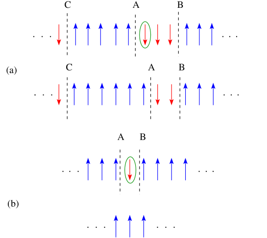
Figure 8: A schematic picture of the dynamics taking place in the model proposed in soham_ps2009 . (a) Case I: Here, the highlighted spin changes its state as the neighbouring domain of down spins is of size two while the size of the other neighbouring domain of up spins is five. Equivalently, in the walker picture, the interface $A$ moves towards $B$, which is closer to it compared to $C$.
(b) Case II: When a down (up) spin is sandwiched between up (down) spins, it will always flip which leads to annihilation of $A$ and $B$.

References

- (1) Privman V., ed. Nonequilibrium Statistical Mechanics in One Dimension, Cambridge University Press, Cambridge (1997).
- (2) Ligget T. M., Interacting Particle Systems, Springer-Verlag, New York, (1985).
- (3) Krapivsky P. L., Redner S. and Ben-Naim E., A Kinetic View of Statistical Physics, Cambridge University Press, Cambridge (2009).
- (4) Odor G., Rev. Mod. Phys. 76, 663 (2004).
- (5) Derrida B., J. Phys. A Math. Gen. 28, 1481 (1995).
- (6) Racz Z., Phys. Rev. lett. 55, 1707 (1985).
- (7) Amar J. G. and Family F., Phys. Rev. A 41, 3258 (1990).
- (8) ben-Avraham D., Burschka M. A., and Doering C. R., J. Stat. Phys. 60, 695 (1990).
- (9) Alcaraz F. C., Droz M., Henkel M. and Rittenberg V. , Ann. Phys. 230, 250 (1994).
- (10) Krebs K., Pfannmuller M. P., Wehefritz B. and Hinrinchsen H. , J. Stat. Phys. 78, 1429 (1995).
- (11) Santos J. E., Schutz G. M. and Stinchcombe R. B., J. Chem. Phys. 105, 2399 (1996).
- (12) Schutz G. M., Z. Phys. B 104, 583 (1997).
- (13) de Oliveira M. J., Brazilian Journal of Physics, 30 128 (2000).
- (14) Kang K. and Redner S., Phys. Rev. A 30, 2833 (1984); 32, 435 (1985).
- (15) Peliti L., J. Phys. A 19, L365 (1986).
- (16) Zumofen G., Blumen A. and Klafter J., J. Chem. Phys. 82, 3198 (1985).
- (17) Droz M. and Sasvari L., Phys. Rev. E 48, R2343 (1993).
- (18) Krapivsky P. L. and Ben-Naim E., Phys. Rev. E 56, 3788 (1997).
- (19) Ben-Naim E., Redner S. and Leyvraz F., Phys. Rev. Lett. 70, 1890 (1993).
- (20) Krapivsky L. and Sire C., Phys. Rev. Lett. 86, 2494 (2001).
- (21) Albano E. V., J. Phys. A: Math. Gen. 24, 3351 (1991).
- (22) Ben-Naim E., Krapivsky P. L. and Randon-Furling J., J. Phys. A: Math. Theor. 49, 205003 (2016).
- (23) Biswas S., Sen P. and Ray P., J. Phys.: Conf. Ser. 297, 012003 (2011).
- (24) Sen P. and Ray P., Phys. Rev. E 92, 012109 (2015).
- (25) Daga B. and Ray P., Phys. Rev. E 99, 032104 (2019).
- (26) Mullick P. and Sen P., Phys. Rev. E 99, 052123 (2019).
- (27) Biswas S. and Sen P. , Phys. Rev. E 80, 027101 (2009).