Meson-meson scattering in two-dimensional QCD

Abstract

We extend the formalism pioneered by Callan, Coote and Gross to investigate the meson-meson scattering within the framework of ’t Hooft model, i.e., the two-dimensional QCD in the $N_{c}\to\infty$ limit. We derive the analytic expressions for various two-body meson-meson scattering amplitudes, concentrating on those quark diagrams which may be identified as the meson-meson contact interaction vertex in the context of the mesonic effective lagrangian in $1/N_{c}$ expansion. We also carry out a detailed numerical study for the meson-meson scattering for various quark flavors, and observe the near-threshold enhancement in some channels. This may be viewed as the hint of the existence of the tetra-quark state below two-meson threshold.

I Introduction

The idea about the existence of the exotic hadrons, such as tetraquark or pentaquark states, is as old as the naive quark model. In recent years, this idea has actively revived as a dozen of new resonances were established experimentally, some of which seem not to fit in the conventional $q\bar{q}$ or $qqq$ states (for a recent review, see Ref. [1, 2]). Most newly observed resonances are closely tied with the charmonium family, generally referred to as the $XYZ$ states. Some of them are considered as the viable candidates for the tetraquark or hadronic molecule.

The tetraquark states are usually studied within phenomenological models such as the QCD sum rules or diquark model [3, 4]. Unfortunately, the connection between these phenomenological approaches and the first principles of QCD appears to be obscure. Recently, the LHCb experiment has discovered the long-awaited doubly-charm baryon $\Xi_{cc}^{++}=ccu$ [5]. Inspired by this important discovery, and with the guidance of heavy quark symmetry, there have been convincing theoretical arguments that the stable doubly-beauty tetraquark states, as exemplified by the $bb\bar{u}\bar{d}$, must exist [6, 7].

The $1/N_{c}$ expansion has historically served an influential nonperturbative tool of QCD [8]. This approach can successfully capture some gross traits of hadron phenomenology, for instance the OZI rule and Regge behavior [9]. In the $N_{c}\to\infty$ limit, the QCD dynamics is dictated by the planar diagrams, and one can show that all the mesons are stable and non-interacting with each other in the limit of infinite number of color. In fact, the meson-meson scattering first starts at order $1/N_{c}$. In his famous series of Erice lectures, Coleman claimed that the quark correlators possessing the tetraquark quantum number make meson pairs and nothing else, as the connected tetraquark diagrams are relatively $1/N_{c}$ suppressed [10]. Consequently there arises no nontrivial tetraquark state in the large-$N_{c}$ limit. However, in 2013 Weinberg [11] scrutinized Coleman’s argument and pointed out some loophole. Weinberg argued that the relatively $1/N_{c}$ suppression does not necessarily rule out the existence of the tetraquark. He concluded that the existence of a narrow tetraquark is not incompatible with large-$N_{c}$ QCD (for some further development along this direction, see for instance [12, 13, 14, 15]).

It is natural to speculate how to validate Weinberg’s tetraquark state from the phenomenological angle. It appears most appealing to search for these states by examining the meson-meson scattering within certain energy range. These states may show up as a Breit-Wigner peak or manifest themselves through some near-threshold enhancement on line-shape.

Albeit being qualitatively successful, the $1/N_{c}$ expansion can hardly make any concrete quantitative prediction in the $3+1$-dimensional QCD. Nevertheless, since the renowned work by ’t Hooft in 1974 [16], it becomes widely known that QCD in the $1+1$ spacetime dimension (hereafter the ’t Hooft model) is a solvable model of great value, which mimics the realistic QCD in many aspects, such as the color confinement, Regge behavior, chiral symmetry breaking and so on. The ’t Hooft model can be viewed as a fruitful theoretical laboratory to test many interesting ideas in realistic QCD. It is the very goal of this paper to carry out a systematic study of the meson-meson scattering in the ’t Hooft model, with the particular incentive of searching for Weinberg’s tetraquark state. In an influential work by Callan, Coote and Gross [17], the theoretical framework of computing the meson decay amplitude has been laid down using the formalism of the Bethe-Salpeter equation. We will closely follow the recipe outlined in [17], and extend their work to the situation for the meson-meson scattering. It is our hope that our result may shed some light on hunting the possible tetraquark states in realistic QCD.

We remark that the meson-meson scattering has already been analyzed within the ’t Hooft model by Batiz, Pena and Stadler more than a decade ago  [18]. Those authors claim to discover a Breit-Wigner peak, which is interpreted as the a $\sigma$-like tetraquark state. Unfortunately, the authors of [18] appear to neglect some important class of Feynman diagrams also of the order $1/N_{c}$, and consequently, their expressions are in fact gauge-dependent and sensitive to the infrared regulator. Therefore, we feel obligated to revisit the meson-meson scattering in the ’t Hooft model from more consistent approach, and consider all possible types of flavor textured possessed by the incident and outgoing mesons.

In the next-to-leading order in $1/N_{c}$ expansion, the relevant Feynman diagrams for meson-meson scattering include all the planar diagrams with the quark line in the edges. As advocated by Witten [9], the equivalent description of $1/N_{c}$ expansion is to treat the meson as the effective degrees of freedom. In this language, the two-body meson scattering process can be classified into two classes of diagrams at tree level. One type is composed of the meson exchange diagram, the other involves a single contact interaction vertex. While the intermediate state of the $s$-channel meson exchange diagram only contains an ordinary $q\bar{q}$ resonance, the latter type of diagram may well accommodate a compact tetraquark structure. Therefore, we will simply suppress those meson exchange diagrams, and concentrate on the contact interaction diagrams to search for the exotic states. The numerical studies reveal that we do not observe any Breit-Wigner resonance, in contradiction with what is found in [18]. Nevertheless, we do observe the near-threshold enhancement in the contact interaction amplitude in some scattering channels. We tend to suggest that this near-threshold enhancement may indicate the existence of some tetraquark structure below the threshold.

The rest of the paper is structured as follows. In Sec. ii@, we recapitulate the essential ingredient of the ’t Hooft model, and review the formalism developed in [17] on quark-antiquark scattering amplitude. In Sec. iii@ we rederive the decay amplitude for a meson to two mesons, within the framework of Callan, Coote and Gross. In Sec. iv@, following the recipe of [17], we derive the analytic expressions for the contact interaction amplitude affiliated with the meson-meson scattering with different flavors. In Sec. v@ we present our numerical results. We summarize in Sec. vi@. In appendix A, we describe some useful light-cone kinematics. IN appendix B, we enumerate the expressions for the contact interaction amplitudes with all possible flavor structures.

II Quark-anti quark scattering in ’t Hooft model

The ’t Hooft model is the two-dimensional QCD where the number of colors is taken to be infinity [16]. The ${\rm QCD}_{2}$ Lagrangian reads

$$\mathcal{L}=-\frac{1}{4}G^{a}_{\ \mu\nu}G^{a\mu\nu}\ +\sum_{f}\bar{q}_{f}(i\gamma^{\mu}D_{\mu}-m_{f})q_{f},$$ (1)

where the sum is extended over quark flavors, and

$$G^{a}_{\mu\nu} = \partial_{\mu}A^{a}_{\nu}-\partial_{\nu}A^{a}_{\mu}+ig_{s}f^{abc}A^{b}_{\mu}A^{c}_{\nu},$$

$$D_{\mu} = \partial_{\mu}-ig_{s}A^{a}_{\mu}T^{a},$$

$$a = 1,2,\ldots,N_{c}^{2}-1,\qquad f=u,d,s,c,b$$ (2)

The Lorentz indices $\mu,\nu$ run from $0$ to $1$. $T^{a}$ are the $SU(N_{c})$ generators, normalized as $tr\left[T^{a}T^{b}\right]=\frac{1}{2}\delta^{ab}$, and $f^{abc}$ denotes the structure constant. The quantization of ${\rm QCD}_{2}$ becomes particularly tractable if the light-cone gauge is imposed:

$$A_{-}=A^{+}=0,$$ (3)

where $A_{-}=\frac{1}{\sqrt{2}}(A^{0}+A^{1})=\frac{1}{\sqrt{2}}(A_{0}-A_{1})$. A particular merit of the light-cone gauge is that the non-ableian component of the field strength simply vanishes, and the nonvanishing field strength tensors are just

$$G_{+-}=-G_{-+}=-\partial_{-}A_{+},$$ (4)

and the Lagrangian can then be written as

$$\mathcal{L}_{{\rm QCD}_{2}}=\frac{1}{2}\mbox{Tr}(\partial_{-}A_{+})^{2}+\sum_{f}\bar{q}_{f}(i\partial_{+}\gamma_{-}+i\partial_{-}\gamma_{+}+{g_{s}}\gamma_{-}A_{+}-m_{f})q_{f}.$$ (5)

The light-cone representation for the Dirac $\gamma$ matrices obeys

$$\gamma^{+}=\frac{1}{\sqrt{2}}(\gamma^{0}\pm\gamma^{1}),\ \ (\gamma^{+})^{2}=(\gamma^{-})^{2}=0,\ \ \{\gamma^{+},\gamma^{-}\}=2.$$ (6)

In the light-cone gauge, there is neither occurrence of the ghost, nor the physical (transverse) gluonic degrees of freedom. We present the Feynman rules in the light-cone gauge in Fig. 1.

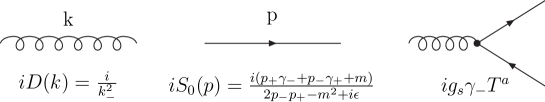
Figure 1: Feynman rules of ${\rm QCD}_{2}$ in the light-cone gauge.

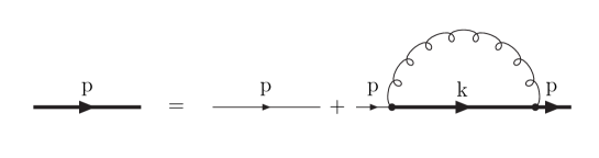
Figure 2: The Dyson-Schwinger equation for the quark self-energy. The thin line denotes the bare quark propagator and the solid line denotes the dressed quark propagator.

The quark self-energy diagrams satisfy the Dyson-Schwinger equation, are depicted in Fig. 2. Notice diagrams with crossed gluons will be suppressed by $1/N_{c}$, therefore the rainbow approximation becomes exact in the large $N_{c}$ limit. The Dyson-Schwinger equation then reads [16, 18]

$$S(p)=S_{0}(p)+i\frac{N_{c}g^{2}_{s}}{2}S(p)\left[\int\frac{d^{2}k}{(2\pi)^{2}}D(p-k)\gamma_{-}S(k)\gamma_{-}\right]S_{0}(p),$$ (7)

where $S(p)$ denotes the dressed quark propagator. We assume $g_{s}\sim\frac{1}{\sqrt{N_{c}}}$, so that $\frac{N_{c}g^{2}_{s}}{2}$ is kept fixed. The solution to the above equation reads

$$S(p) = \frac{p_{-}\gamma_{+}}{2p_{+}p_{-}-M^{2}-\frac{N_{c}g_{s}^{2}}{2\pi}\frac{|p_{-}|}{\rho}+i\epsilon},$$

$$M^{2} = m^{2}-\frac{N_{c}g_{s}^{2}}{2\pi},$$ (8)

where $M$ denotes the mass of the dressed quark. $\rho$ is a dimensionful cutoff introduced to regularize the infra-red divergence in the loop integral. For the loop integral appearing in Fig. 2, the value of $\rho$ is taken such that $\rho<|k_{-}|<\infty$.

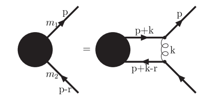
Figure 3: The Bethe-Salpeter equation for the $q\bar{q}$bound state.

With the dressed quark propagator available, one then proceed to write the bound state equation for the $q\bar{q}$ pair. In the large $N_{c}$ limit, the ladder approximation in Bethe-Salpeter equation becomes exact, as shown in Fig. 3. The corresponding Bethe-Salpeter equation reads

$$\psi(p,r) = 2iN_{c}g_{s}^{2}p_{-}(p_{-}-r_{-})\left[2p_{+}p_{-}-M_{1}^{2}-\frac{N_{c}g_{s}^{2}}{2\pi}\frac{|p_{-}|}{\rho}+i\epsilon\right]^{-1}$$ (9)

$$\times\left[2(p_{+}-r_{+})(p_{-}-r_{-})-M_{2}^{2}-\frac{N_{c}g_{s}^{2}}{2\pi}\frac{|p_{-}-r_{-}|}{\rho}+i\epsilon\right]^{-1}$$

$$\times\int\frac{d^{2}k}{(2\pi)^{2}}\frac{1}{k_{-}^{2}}\psi(p+k,r).$$

Defining $\varphi(p_{-},r)\equiv\int dp_{+}\psi(p,r)$, one then obtains

$$\varphi(p_{-},r) = i\frac{N_{c}g_{s}^{2}}{2(2\pi)^{2}}\int dp_{+}\left[p_{+}-\frac{M_{1}^{2}}{2p_{-}}-\frac{N_{c}g_{s}^{2}}{4\pi}\frac{\operatorname{sgn}(p_{-})}{\rho}+i\epsilon\cdot\operatorname{sgn}(p_{-})\right]^{-1}$$ (10)

$$\times \left[p_{+}-r_{+}-\frac{M_{2}^{2}}{2(p_{-}-r_{-})}-\frac{N_{c}g_{s}^{2}}{4\pi}\frac{\operatorname{sgn}(p_{-}-r_{-})}{\rho}+i\epsilon\cdot\operatorname{sgn}(p_{-}-r_{-})\right]^{-1}$$

$$\times \int dk_{-}\frac{\varphi(p_{-}+k_{-},r)}{k_{-}^{2}}.$$

Completing the $p_{+}$ integral and using

$$\int dk_{-}\frac{\varphi(p_{-}+k_{-},r)}{k_{-}^{2}}=\frac{2}{\rho}\varphi(p_{-},r)+P\int dk_{-}\frac{\varphi(p_{-}+k_{-},r)}{k_{-}^{2}},$$ (11)

where $P\frac{1}{k_{-}^{2}}=\frac{1}{2}(\frac{1}{(k_{-}+i\epsilon)^{2}}+\frac{1}{(k_{-}-i\epsilon)^{2}})$ indicates a principle-value prescription, one then finds

$$\left[r_{+}-\frac{M_{2}^{2}}{2(r_{-}-p_{-})}-\frac{M_{1}^{2}}{2p_{-}}-\frac{N_{c}g_{s}^{2}}{2\pi\rho}+i\epsilon\right]\varphi(p_{-},r)$$ (12)

$$= -\frac{N_{c}g_{s}^{2}}{4\pi}\theta(p_{-})\theta(r_{-}-p_{-})\times\left[\frac{2}{\rho}\varphi(p_{-},r)+P\int dk_{-}\frac{\varphi(p_{-}+k_{-},r)}{k_{-}^{2}}\right].$$

Clearly, the infra-red singularities in both sides cancel with each other. After multiplying the factor $\frac{4\pi}{N_{c}g_{s}^{2}}r_{-}$ onto both sides of the above equation, and introducing the following symbols:

$$\mu^{2}=\frac{4\pi r_{+}r_{-}}{N_{c}g_{s}^{2}},\qquad\alpha_{1,2}=\frac{2\pi M_{1,2}^{2}}{N_{c}g_{s}^{2}},\qquad x=\frac{p_{-}}{r_{-}},$$ (13)

one then recovers the celebrated ’t Hooft equation:

$$\mu^{2}\varphi(x)=\left(\frac{\alpha_{1}}{x}+\frac{\alpha_{2}}{1-x}\right)\varphi(x)-P\int_{0}^{1}dy\frac{\varphi(y)}{(x-y)^{2}}.$$ (14)

The solution of the ’t Hooft equation leads to discrete mass enginevalues $\mu_{n}^{2}$ ($n=0,1,2,\cdots$) for color-singlet mesons. The corresponding wave functions $\varphi_{n}$ satisfy the completeness and orthogonality relations:

$$\sum_{n}\varphi_{n}(x)\varphi_{n}^{\ast}(x^{\prime})=\delta(x-x^{\prime}),\ \ \ \ \ \int_{0}^{1}\varphi_{n}^{\ast}(x)\varphi_{m}(x)dx=\delta_{nm}.$$ (15)

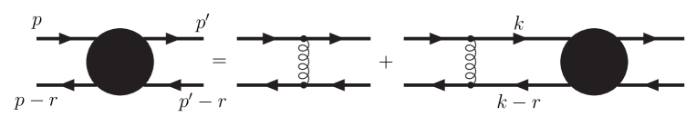
Figure 4: The Bethe-Salpeter equation for quark-antiquark scattering amplitude.

In a similar vein, one may write down the Bethe-Salpeter equation for the quark-antiquark scattering amplitude. As indicated in Fig. 4, the corresponding inhomogeneous Bethe-Salpeter equation reads [17]

$$\mathcal{T}(p,p^{\prime};r)=-\frac{ig_{s}^{2}}{2(p_{-}-p_{-}^{\prime})^{2}}+i2N_{c}g_{s}^{2}\int\frac{d^{2}k}{(2\pi)^{2}}\frac{1}{(k_{-}-p_{-})^{2}}\tilde{S}(k)\tilde{S}(k-r)\mathcal{T}(k,p^{\prime};r),$$ (16)

with $\tilde{S}(p)\gamma_{+}=S(p)$. This solution reads

$$\mathcal{T}(x,x^{\prime};r) = -\frac{ig_{s}^{2}}{2r_{-}^{2}(x-x^{\prime})^{2}}+\sum_{n}\frac{i}{r^{2}-r_{n}^{2}}\left\{\varphi_{n}(x)\frac{g_{s}^{2}}{2|r_{-}|}\sqrt{\frac{N_{c}}{\pi}}\left[\theta(x(1-x))\frac{2|r_{-}|}{\rho}+\frac{\alpha_{1}}{x}+\frac{\alpha_{2}}{1-x}-\mu_{n}^{2}\right]\right\}$$ (17)

$$\times\left\{\varphi_{n}^{\ast}(x^{\prime})\frac{g_{s}^{2}}{2|r_{-}|}\sqrt{\frac{N_{c}}{\pi}}\left[\theta(x^{\prime}(1-x^{\prime}))\frac{2|r_{-}|}{\rho}+\frac{\alpha_{1}}{x^{\prime}}+\frac{\alpha_{2}}{1-x^{\prime}}-\mu_{n}^{2}\right]\right\},$$

where $x=\frac{p_{-}}{r_{-}},\ \ x^{\prime}=\frac{p_{-}^{\prime}}{r_{-}}.$ The amplitude bears infinite towers of poles located at $r^{2}=r_{n}^{2},\ n=0,1,2\cdots$. The physical interpretation of the above solution is clear, that the summation of the $t$-channel multi-gluon exchange is equivalent to the summation of the $s$-channel exchange of the quark-antiquark bound state. The residue of the pole gives the meson-$q\bar{q}$ vertex function [19]:

$$\Phi^{1,2}_{n}(x)=\varphi_{n}(x)\frac{g_{s}^{2}}{2|r_{-}|}\sqrt{\frac{N_{c}}{\pi}}\left[\theta(x(1-x))\frac{2|r_{-}|}{\rho}+\frac{\alpha_{1}}{x}+\frac{\alpha_{2}}{1-x}-\mu_{n}^{2}\right].$$ (18)

The functions $\Phi^{1,2}_{n}(x)$ can be interpreted as the transition amplitude between the meson and the quark-antiquark pair, which serves an essential ingredient in our calculation for the meson-meson scattering.

III Two-body strong decay of the meson

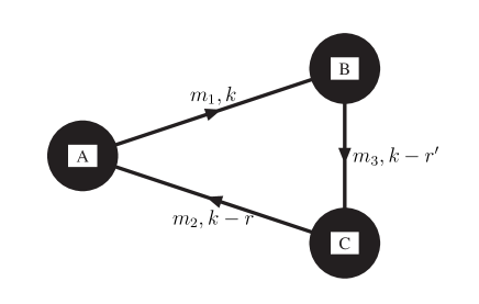
Figure 5: A two-body decay $A\rightarrow B+C$. $r$ is the incoming momentum of A, $r^{\prime}$ is the outgoing momentum of B, and $r^{\prime\prime}=r-r^{\prime}$ is the outgoing momentum of C.

In this section, we take the two-body decay of the meson in ’t Hooft model as a warm-up exercise. A mesonic two-body decay diagram is shown in Fig. 5. The decay amplitude can be written as

$$i\mathcal{M}(A\to BC) = -iN_{c}\int\frac{d^{2}k}{(2\pi)^{2}}\frac{\Phi_{A}^{1,2}(x_{A})\Phi_{B}^{1,3}(x_{B})\Phi_{C}^{3,2}(x_{C})}{k_{+}-\frac{M_{1}^{2}}{2k_{-}}-\frac{N_{c}g_{s}^{2}}{4\pi}\frac{\operatorname{sgn}(k_{-})}{\rho}+i\varepsilon\cdot\operatorname{sgn}(k_{-})}$$ (19)

$$\times \frac{1}{k_{+}-r_{+}-\frac{M_{2}^{2}}{2(k_{-}-r_{-})}-\frac{N_{c}g_{s}^{2}}{4\pi}\frac{\operatorname{sgn}(k_{-}-r_{-})}{\rho}+i\varepsilon\cdot\operatorname{sgn}(k_{-}-r_{-})}$$

$$\times \frac{1}{k_{+}-r^{\prime}_{+}-\frac{M_{3}^{2}}{2(k_{-}-r^{\prime}_{-})}-\frac{N_{c}g_{s}^{2}}{4\pi}\frac{\operatorname{sgn}(k_{-}-r^{\prime}_{-})}{\rho}+i\varepsilon\cdot\operatorname{sgn}(k_{-}-r^{\prime}_{-})}.$$

where $r$ is the incoming momentum of particle $A$, and $r^{\prime}$ is the outgoing momentum of particle $B$. The arguments of the $\Phi$ functions are defined as

$$x_{A}=\frac{k_{-}}{r_{-}},\ \ \ \ x_{B}=\frac{k_{-}}{r_{-}^{\prime}},\ \ \ \ x_{C}=\frac{k_{-}-r_{-}^{\prime}}{r_{-}-r_{-}^{\prime}}.$$ (20)

One can first carry out the $k_{+}$ integral and take $\rho\rightarrow 0$ finally as the decay amplitude is infra-red safe. In doing that, one should note that at least one of the $x_{A,B,C}$ can not lie in the region $0<x<1$ due to the momentum conversation. The final expression for the decay amplitude reads

$$i\mathcal{M}(A\to BC) = -g_{s}^{2}\sqrt{N_{c}/\pi}\left[\frac{1}{1-\omega}\int_{0}^{\omega}dx\varphi_{A}\left(x\right)\varphi_{B}\left(\frac{x}{\omega}\right)\tilde{\Phi}_{C}(\frac{\omega-x}{\omega-1})\right.$$ (21)

$$\left.-\frac{1}{\omega}\int_{\omega}^{1}dx\varphi_{A}\left(x\right)\tilde{\Phi}_{B}(\frac{x}{\omega})\varphi_{C}\left(\frac{\omega-x}{\omega-1}\right)\right],$$

where we define $\omega=\frac{r_{-}^{\prime}}{r_{-}}$, $x=x_{A}$, and $\tilde{\Phi}_{C,B}(x)=\int_{0}^{1}dy\frac{\varphi_{C,B}(y)}{(x-y)^{2}}$. This result has already been obtained by Barbon and companions [20] long ago, which yet takes a different route, i.e., using the Hamiltonian and bosonization approach. The numerical study of the various decay amplitudes have also been conducted by Abdalla and collaborators [21].

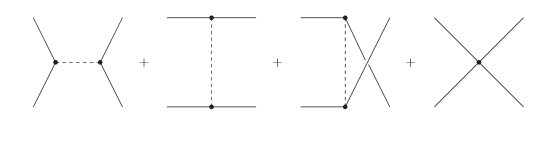
Figure 6: The tree diagrams for the scattering process $A+B\rightarrow C+D$, where the dashed line represents the exchanged meson. A sum over all species of mesons is understood.

IV The meson-meson scattering

In this section, we will derive the analytical results for the meson-meson scattering in the ’t Hooft model. Consider the meson-meson scattering $A+B\rightarrow C+D$, as Witten has illustrated in Ref. [9], in the large $N_{c}$ limit the leading contribution comes from the tree diagrams as shown in Fig. 6. These tree diagrams can be classified into two types, the contact-interaction type and the meson-exchange type. To look for the exotic structure, we focus on the contact interaction type diagrams in this work, because the meson exchange diagrams contain only ordinary $q\bar{q}$ mesons. To figure out the contact interaction amplitude in the t’ Hooft model, one needs to specify the flavor structure in the scattering. Let’s first consider the scattering which contain three different flavors $A(a\bar{b})+B(c\bar{a})\rightarrow C(a\bar{b})+D(c\bar{a})$(where $a,b,c$ denotes the quarks’ flavors ). At the leading order, i.e., order $1/N_{c}$, there are infinite Feynman diagrams. We show three of them in Fig. 7, which are the box diagram form by the quark lines and the box diagrams with additional one gluon exchange. The black bubble in Fig. 7 represents the meson-$q\bar{q}$ vertex function $\Phi^{q,\bar{q}}_{n}(x)$, thus diagrams with gluon exchange between adjacent quark lines are also included. Other diagrams which are also at the leading order and not shown in Fig 7 are those with multi-gluon exchange in ladder fashion between nonadjacent quark lines. As addressed in the above, the summation of the multi-gluon exchange diagrams is equivalent to the summation of the $q\bar{q}$ meson exchange diagrams, thus the sum of the infinite multi-gluon exchange diagrams can be converted to the sum of the meson exchange diagrams as shown in Fig. 6(one can refer to Ref. [17] for more detail). Therefore we only have to consider the diagrams in Fig. 7, as their sum equals to the contact interaction term. We take Fig. 7(a) as an example to show some of the details in our calculations. The amplitude for Fig. 7(a) reads

$$i\mathcal{M}_{box} = N_{c}\int\frac{d^{2}k}{(2\pi)^{2}}\frac{\Phi_{A}^{a,b}(x_{A})\Phi_{B}^{c,a}(x_{B})\Phi_{C}^{a,b}(x_{C})\Phi_{D}^{c,a}(x_{D})}{k_{+}-\frac{M_{a}^{2}}{2k_{-}}-\frac{N_{c}g_{s}^{2}}{4\pi}\frac{\operatorname{sgn}(k_{-})}{\rho}+i\varepsilon\cdot\operatorname{sgn}(k_{-})}$$ (22)

$$\times \frac{1}{k_{+}+r_{B+}-\frac{M_{c}^{2}}{2(k_{-}+r_{B-})}-\frac{N_{c}g_{s}^{2}}{4\pi}\frac{\operatorname{sgn}(k_{-}+r_{B-})}{\rho}+i\varepsilon\cdot\operatorname{sgn}(k_{-}+r_{B-})}$$

$$\times \frac{1}{k_{+}+r_{B+}-r_{D+}-\frac{M_{a}^{2}}{2(k_{-}+r_{B-}-r_{D-})}-\frac{N_{c}g_{s}^{2}}{4\pi}\frac{\operatorname{sgn}(k_{-}+r_{B-}-r_{D-})}{\rho}+i\varepsilon\cdot\operatorname{sgn}(k_{-}+r_{B-}-r_{D-})}$$

$$\times \frac{1}{k_{+}-r_{A+}-\frac{M_{b}^{2}}{2(k_{-}-r_{A-})}-\frac{N_{c}g_{s}^{2}}{4\pi}\frac{\operatorname{sgn}(k_{-}-r_{A-})}{\rho}+i\varepsilon\cdot\operatorname{sgn}(k_{-}-r_{A-})},$$

where

$$x_{A}=\frac{k_{-}}{r_{A-}},\ \ \ x_{B}=\frac{k_{-}+r_{B-}}{r_{B-}},\ \ \ x_{C}=\frac{k_{-}+r_{B-}-r_{D-}}{r_{C-}},\ \ \ x_{D}=\frac{k_{-}+r_{B-}}{r_{D-}}.$$ (23)

We can first carry out the $k_{+}$ integral and expand the expression in power of $\rho$, as we will postpone $\rho\rightarrow 0$ finally. In doing the $k_{+}$ residual integral one should keep in mind that $x_{A}$($x_{C}$) and $x_{B}$($x_{D}$) cannot lie in the region $0<x<1$ simultaneously, we can then find that Fig.7(a) is of the order $\mathcal{O}(\rho)$. Therefore Fig.7(a) gives vanishing contribution after taking the limit $\rho\rightarrow 0$. One can easily check that Fig.7(b) also gives vanishing contribution due to the same reason. In contrast $x_{A}$($x_{C}$) and $x_{B}$($x_{D}$) can lie in the region $0<x<1$ simultaneously in Fig. 7(c), and this diagram gives nonvanishing contribution. The difference between Fig. 7(c) and the other two diagrams is that the S-channel cut line of this diagram contains $q\bar{q}g$ state, while others contain only the $q\bar{q}$ state. The final expression for Fig. 7 reads

$$i\mathcal{M} = (1+\mathcal{C})i\mathcal{M}_{0},$$

$$i\mathcal{M}_{0} = \theta(\omega_{2}-\omega_{1})i2g_{s}^{2}\omega_{1}\int_{0}^{1}dx\int_{0}^{1}dy\frac{1}{(y\omega_{1}-\omega_{2}-x)^{2}}\varphi_{A}\left(\frac{\omega_{2}-\omega_{1}+x}{\omega_{2}-\omega_{1}+1}\right)\varphi_{B}\left(y\right)\varphi_{C}\left(x\right)\varphi_{D}\left(\frac{y\omega_{1}}{\omega_{2}}\right),$$

where $\omega_{1}=\frac{r_{B-}}{r_{C-}},\omega_{2}=\frac{r_{D-}}{r_{C-}}$ and

$$\mathcal{C}=(A\leftrightarrow C,\ \ B\leftrightarrow D,\ \ \omega_{1}\rightarrow\frac{\omega_{2}}{1+\omega_{2}-\omega_{1}},\ \ \omega_{2}\rightarrow\frac{\omega_{1}}{1+\omega_{2}-\omega_{1}}).$$ (25)

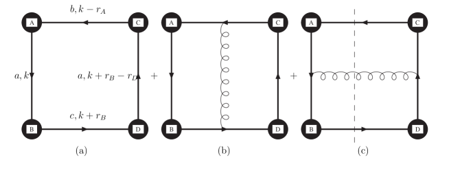
Figure 7: Four-body contact interaction part for $A(a\bar{b})+B(c\bar{a})\rightarrow C(a\bar{b})+D(c\bar{a})$. $r_{A},r_{B}$ are the incoming momenta of A and B respectively, and $r_{C},r_{D}$ are the outgoing momenta of C and D respectively. The dashed line is the cut line.

The results for the four different flavor are similar. We then come to study the meson-meson scattering for other flavor structures. We find that there are more Feynman diagrams involved for meson-meson scatterings with less flavor. The box diagrams for the two-flavor scattering $A(a\bar{b})+B(b\bar{a})\rightarrow C(a\bar{b})+D(b\bar{a})$ are shown in Fig. 9. One can see that there are two box diagrams in the two-flavor scattering. To calculate the contact interaction, the box diagrams with additional one gluon exchange should also be included. Again, only diagrams with S-channel cuts containing quark-gluon-anti quark states give nonvanishing contribution. The final expression of the contact interaction for $A(a\bar{b})+B(b\bar{a})\rightarrow C(a\bar{b})+D(b\bar{a})$ reads

$$i\mathcal{M}=(1+\mathcal{P})(1+\mathcal{C})i\mathcal{M}_{0},$$ (26)

where $\mathcal{C}$ is defined above, and the operation $\mathcal{P}$ is defined as $\mathcal{P}=(A\leftrightarrow B,\ \ C\leftrightarrow D,\ \ \omega_{1}\rightarrow\frac{1+\omega_{2}-\omega_{1}}{\omega_{2}},\ \ \omega_{2}\rightarrow\frac{1}{\omega_{2}})$.

For the single-flavor scattering $A(a\bar{a})+B(a\bar{a})\rightarrow C(a\bar{a})+D(a\bar{a})$, there are six box diagrams. We show three of them in Fig. 10, and others are corresponding diagrams with clockwise fermion loops. To calculate the contact interaction, we also need to consider the box diagrams with additional one gluon exchange. Thus we need to consider 18 diagrams in the single-flavor scattering. We note that while Fig. 10(a,b) give vanishing contribution, Fig. 10(c) gives nonvanishing contribution. This difference is due to the fact that the two incoming particles $A$ and $B$ are directly connected by quark line in Fig. 10(a,b) but not in Fig. 10(c). In other words, all the S-channel cuts in Fig. 10(c) contain tetraquark states. We conclude that Feynman diagram with the S-channel cut line containing only the $q\bar{q}$ state gives vanishing contribution. Therefore, 10 of the 18 diagrams give nonvanishing contributions. The calculation is tedious but straightforward. The only subtlety is that the amplitude for Fig. 10(c) contains the divergent part $\mathcal{O}(1/\rho)$, and the divergent part can be exactly canceled by the contributions from the corresponding diagrams with additional one gluon exchange [17]. The final expression for the contact interaction of $A(a\bar{a})+B(a\bar{a})\rightarrow C(a\bar{a})+D(a\bar{a})$ reads

$$i\mathcal{M}=(1+\mathcal{R})(1+\mathcal{P})(1+\mathcal{C})i\mathcal{M}_{0}+(1+\mathcal{R})i\mathcal{M}_{1},$$ (27)

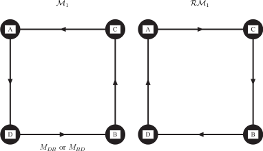
Figure 8: The Feynman diagrams for $\mathcal{M}_{1}$ and $\mathcal{RM}_{1}$, where $M_{DB}$($M_{BD}$) indicates the $M$ of the quark connecting $B$ meson and $D$ meson.

where

$$i\mathcal{M}_{1} = -(1+\mathcal{Q})\theta(1-\omega_{1})i2g_{s}^{2}\int_{0}^{1}dxP\int_{0}^{1}dy\frac{\omega_{1}\omega_{2}}{[(y-1)\omega_{1}+(1-x)\omega_{2}]^{2}}\varphi_{A}\left(\frac{x\omega_{2}}{1+\omega_{2}-\omega_{1}}\right)\varphi_{B}\left(y\right)\varphi_{C}\left(y\omega_{1}\right)\varphi_{D}\left(x\right)$$

$$-(1+\mathcal{C})\theta(\omega_{2}-\omega_{1})i2g_{s}^{2}\int_{0}^{1}dxP\int_{0}^{1}dy\frac{\omega_{1}}{(y\omega_{1}-x)^{2}}\varphi_{A}\left(\frac{x+\omega_{2}-\omega_{1}}{1+\omega_{2}-\omega_{1}}\right)\varphi_{B}\left(y\right)\varphi_{C}\left(x\right)\varphi_{D}\left(\frac{(y-1)\omega_{1}+\omega_{2}}{\omega_{2}}\right)$$

$$-(1+\mathcal{Q}+\mathcal{P}+\mathcal{C})\theta(\omega_{2}-\omega_{1})\theta(\omega_{1}-1)i\frac{4\pi}{N_{c}}\int_{0}^{1}dx\left[2r_{C+}r_{C-}+2r_{D+}r_{C-}+\frac{M_{DB}^{2}}{x-\omega_{1}}+\frac{M_{CA}^{2}}{x-1}\right.$$

$$\left.-\frac{M_{AD}^{2}}{x-\omega_{1}+\omega_{2}}-\frac{M_{BC}^{2}}{x}\right]\times\varphi_{A}\left(\frac{x-\omega_{1}+\omega_{2}}{1+\omega_{2}-\omega_{1}}\right)\varphi_{B}\left(x/\omega_{1}\right)\varphi_{C}\left(x\right)\varphi_{D}\left(\frac{x-\omega_{1}+\omega_{2}}{\omega_{2}}\right),$$

where $M_{DB}$ indicates the $M$, defined in (8), of the corresponding quark propagator connecting the meson $D$ and the meson $B$, so are the terms $M_{CA}$ , $M_{AD}$ and $M_{BC}$. We also have

$$\mathcal{R}=(C\leftrightarrow D,\ \ \omega_{1}\rightarrow\frac{\omega_{1}}{\omega_{2}},\ \ \omega_{2}\rightarrow 1/\omega_{2}),\ \ \ \mathcal{Q}=(B\leftrightarrow C,\ \ A\leftrightarrow D,\ \ \omega_{1}\rightarrow 1/\omega_{1},\ \ \omega_{2}\rightarrow\frac{1+\omega_{2}-\omega_{1}}{\omega_{1}}).$$ (29)

We have shown the Feynman diagrams of $\mathcal{M}_{1}$ and $\mathcal{RM}_{1}$ in Fig.8. If there is an $\mathcal{R}$ acting on the $\mathcal{M}_{1}$, one should refer to the feynman diagram of $\mathcal{RM}_{1}$ to figure out the flavor of the $M$s.

For completeness, we also list the contact interaction terms for meson-meson scatterings with other flavor structures in the appendix. We would like to mention that parts of the analytical results are also given in Ref. [20].

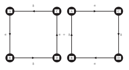
Figure 9: Box diagrams for $A(a\bar{b})+B(b\bar{a})\rightarrow C(a\bar{b})+D(b\bar{a})$.

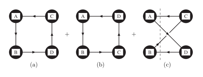
Figure 10: Three Box diagrams for $A(a\bar{a})+B(a\bar{a})\rightarrow C(a\bar{a})+D(a\bar{a})$. Other three diagrams are similar ones but with clockwise fermion loops.

We end this section by commenting on the preceding calculation of meson-meson scattering by Batiz et al. [18]. One of the problems is that their Feynman rules seems not to distinguish the outgoing quark and the incoming quark for a meson vertex. This leads to a nonvanishing result for Fig. 7$(a)$, which is vanishing in our paper. The other severe mistake is that they have missed the one-gluon exchange diagrams. As mentioned before, Fig. 10$(c)$ possesses a term containing factor $\frac{1}{\rho}$, which should be canceled by the corresponding diagrams with an additional gluon exchange diagram. Thus Fig. 10$(c)$ alone is IR divergent. However, since the authors of [18] employed the principle-value as their default IR regulator, they have not realized their results are actually IR divergent. Therefore, their result for Fig. 10$(c)$ cannot be affiliated with physical significance. We stress that, by confirming that our final result is free from the IR cutoff $\rho$, provides a quite nontrivial consistency check for our calculation.

V Numerical results

Figure 11: Amplitudes for the contact term in $A(c\bar{c})+B(c\bar{c})\rightarrow C(c\bar{c})+D(c\bar{c})$.

Figure 12: Amplitudes for the contact term in $A(c\bar{s})+B(c\bar{s})\rightarrow C(c\bar{s})+D(c\bar{s})$.

Figure 13: Amplitudes for the contact term in $A(c\bar{u})+B(c\bar{d})\rightarrow C(c\bar{u})+D(c\bar{d})$.

Figure 14: Amplitudes for the contact term in $A(c\bar{d})+B(b\bar{s})\rightarrow C(b\bar{d})+D(c\bar{s})$.

We now move to the numerical study of the meson-meson scattering. To evaluate the contact interaction amplitude of the meson-meson scattering, we first need the numerical results for the meson light-cone wave functions. These functions can be obtained by solving the ’t Hooft equation with the standard eigenvalue routines [22, 23]. Following Ref. [24], we express any dimensional quantity in unit of $\sqrt{2\lambda}=340$ MeV, where $\lambda=\frac{g_{s}^{2}N_{c}}{4\pi}$. To mimic the realistic meson spectrum in ${\rm QCD}_{4}$, the bare quark masses are chosen as $m_{u}=15.3\textup{MeV},\ m_{d}=30.6\textup{ MeV},\ m_{s}=254\textup{MeV},\ m_{c}=1.44\textup{Gev}$ [24], and $m_{b}=4.61\textup{Gev}$. For the sake of completeness, we show the numerical results for the one-flavor scattering $A(c\bar{c})+B(c\bar{c})\rightarrow C(c\bar{c})+D(c\bar{c})$ in Fig. 11, the two-flavor scattering $A(c\bar{s})+B(c\bar{s})\rightarrow C(c\bar{s})+D(c\bar{s})$ in Fig. 12, the three-flavor scattering $A(c\bar{u})+B(c\bar{d})\rightarrow C(c\bar{u})+D(c\bar{d})$ in Fig. 13, and the four-flavor scattering $A(c\bar{d})+B(b\bar{s})\rightarrow C(b\bar{d})+D(c\bar{s})$ in Fig. 14. For simplicity, we only consider the scattering of the ground-state mesons, which are simply represented by $0+0\rightarrow 0+0$. From our numerical results, we do observe clear enhancement near the threshold. Upon varying the bare quark mass, we find that the near threshold enhancement does not disappear. We also find that this enhancement is not necessary a universal feature for meson-meson scattering. For example, we do not observe the near-threshold enhancement in the channel $A(c\bar{d})+B(b\bar{s})\rightarrow C(b\bar{d})+D(c\bar{s})$.

VI Summary

In summary, we have carried out a comprehensive study on the meson-meson scattering in the ’t Hooft model. Since the original goal is to search for the possible tetraquark state, we intentionally only examine the contact interaction part of the meson-meson scattering amplitude. We derive the analytic results for the corresponding amplitude, considering all possible flavor structures. We find that only Feynman diagrams with the $s$-channel cut on the $q\bar{q}g$ or $q\bar{q}q\bar{q}$ intermediate states can make nonvanishing contribution. Reassuringly, we explicitly verify that the contact interaction amplitude is free from the IR regulator $\rho$. Our numerical study reveals that these diagrams may generate the near-threshold enhancement for some channels of meson-meson scattering. This may be viewed as a sign of the existence of the tetraquark state below threshold.

APPENDIX A: light-cone KINEMATICS

In the $1+1$ dimensional case, there is only one kinematical degree of freedom involved in a $2\to 2$ scattering within the center-of-mass frame. Thus, in principle we can express all the results in terms of the squared center-of-mass energy $s$. Nevertheless, we employ two kinematical variables in our calculations for convenience, which are defined as

$$\omega_{1}=\frac{r_{B-}}{r_{C-}},\ \ \ \omega_{2}=\frac{r_{D-}}{r_{C-}}.\ \ \$$ (30)

with all the final results expressed by $\omega_{1}$ and $\omega_{2}$. To be clear, we also list the following equations

$$\frac{r_{A-}}{r_{B-}}=\frac{1+\omega_{2}-\omega_{1}}{\omega_{1}},\ \frac{r_{D-}}{r_{C-}}=\omega_{2},$$ (31)

with the relations (31) and the light-cone dispersion relation $r_{X+}=\frac{M_{X}^{2}}{2r_{X-}}$, we can transform the following two equations

$$s=2(r_{C+}+r_{D+})(r_{C-}+r_{D-}),$$

$$s=2(r_{A+}+r_{B+})(r_{A-}+r_{B-}),$$

into

$$s\frac{\omega_{2}}{1+\omega_{2}} = M_{C}^{2}\omega_{2}+M_{D}^{2},$$ (32a)

$$s\frac{\omega_{2}}{1+\omega_{2}} = M_{A}^{2}\frac{\omega_{2}}{1+\omega_{2}-\omega_{1}}+M_{B}^{2}\frac{\omega_{2}}{\omega_{1}}.$$ (32b)

which show the relations between $s$ and $\omega$s.

To get real solutions for equations (32), one needs to put $s$ above the threshold $\max\left\{(M_{A}+M_{B})^{2},(M_{C}+M_{D})^{2}\right\}$. Furthermore, once a suitable $s$ is selected, there will be four solutions for $(\omega_{1},\omega_{2})$. The relations between $\omega$s and the direction of mesons’ momentums is shown in Table.1. Since for a specific scattering the incoming momenta are fixed, we choose the first two lines of Table. 1 in our calculation. Besides, it should be mentioned that when $C$ and $D$ are the same mesons, the first two lines of Table.1 are equivalent since the meson $C$ and the meson $D$ are identical particles.

$\omega_{1}$	$\omega_{2}$	A	B	C	D
smaller	smaller	$\rightarrow$	$\leftarrow$	$\rightarrow$	$\leftarrow$
smaller	larger	$\rightarrow$	$\leftarrow$	$\leftarrow$	$\rightarrow$
larger	smaller	$\leftarrow$	$\rightarrow$	$\rightarrow$	$\leftarrow$
larger	larger	$\leftarrow$	$\rightarrow$	$\leftarrow$	$\rightarrow$

Table 1: The relation between $\omega$s and the directions of mesons’ momentums $r^{1}$ in the center-of-mass frame, where $\rightarrow$($\leftarrow$) indicates a positive(negative) $r^{1}$. There are two solutions for each $\omega$, namely four groups of solutions. “Smaller”(“larger”) means that we choose the smaller(larger) $\omega_{1(2)}$.

APPENDIX B: CONTACT INTERACTION TERMS FOR MESON-MESON SCATTERINGS WITH DIFFERENT FLAVOR STRUCTURES

Contact interaction amplitudes for meson-meson scattering with different flavor structures can be expressed with the functions $\mathcal{M}_{0}$ and $\mathcal{M}_{1}$ defined in Sec.iii@.

• Contact interaction terms for meson-meson scatterings with four different flavors:
  

  $$A(a\bar{d})+B(b\bar{a})\rightarrow C(c\bar{d})+D(b\bar{c}) :\ \ (1+\mathcal{C})\mathcal{M}_{0},$$

  $$A(a\bar{d})+B(c\bar{b})\rightarrow C(c\bar{d})+D(a\bar{b}) :\ \ \mathcal{M}_{1}.$$ (33)

• Contact interaction terms for meson-meson scatterings with three different flavors:
  

  $$\begin{array}[]{lllll}&&A(a\bar{c})+B(b\bar{a})\rightarrow C(b\bar{c})+D(b\bar{b})&&:\ \ (1+\mathcal{C})\mathcal{M}_{0},\\ &&A(a\bar{c})+B(b\bar{a})\rightarrow C(c\bar{c})+D(b\bar{c})&&:\ \ (1+\mathcal{C})\mathcal{M}_{0},\\ &&A(a\bar{b})+B(c\bar{a})\rightarrow C(a\bar{b})+D(c\bar{a})&&:\ \ (1+\mathcal{C})\mathcal{M}_{0},\\ &&A(a\bar{b})+B(b\bar{a})\rightarrow C(c\bar{b})+D(b\bar{c})&&:\ \ (1+\mathcal{C})\mathcal{M}_{0},\\ &&A(a\bar{a})+B(b\bar{a})\rightarrow C(c\bar{a})+D(b\bar{c})&&:\ \ (1+\mathcal{C})\mathcal{M}_{0},\\ &&A(a\bar{c})+B(a\bar{a})\rightarrow C(b\bar{c})+D(a\bar{b})&&:\ \ (1+\mathcal{C})\mathcal{M}_{0},\\ &&A(a\bar{c})+B(b\bar{b})\rightarrow C(b\bar{c})+D(a\bar{b})&&:\ \ \mathcal{M}_{1},\\ &&A(a\bar{c})+B(c\bar{b})\rightarrow C(c\bar{c})+D(a\bar{b})&&:\ \ \mathcal{M}_{1},\\ &&A(a\bar{c})+B(a\bar{b})\rightarrow C(a\bar{c})+D(a\bar{b})&&:\ \ \mathcal{M}_{1},\\ &&A(a\bar{c})+B(b\bar{c})\rightarrow C(b\bar{c})+D(a\bar{c})&&:\ \ \mathcal{M}_{1}.\end{array}$$

• Contact interaction terms for meson-meson scatterings with two different flavors:
  

  $$\begin{array}[]{lllll}A(a\bar{a})+B(b\bar{a})\rightarrow C(b\bar{a})+D(b\bar{b})&&:\ \ (1+\mathcal{C})\mathcal{M}_{0},\\ A(a\bar{a})+B(a\bar{a})\rightarrow C(b\bar{a})+D(a\bar{b})&&:\ \ (1+\mathcal{R}\mathcal{P})(1+\mathcal{C})\mathcal{M}_{0},\\ A(a\bar{b})+B(b\bar{a})\rightarrow C(b\bar{b})+D(b\bar{b})&&:\ \ (1+\mathcal{R})(1+\mathcal{C})\mathcal{M}_{0},\\ A(a\bar{b})+B(b\bar{a})\rightarrow C(a\bar{b})+D(b\bar{a})&&:\ \ (1+\mathcal{P})(1+\mathcal{C})\mathcal{M}_{0},\\ A(a\bar{b})+B(a\bar{a})\rightarrow C(b\bar{b})+D(a\bar{b})&&:\ \ (1+\mathcal{C})\mathcal{M}_{0},\\ A(a\bar{a})+B(b\bar{b})\rightarrow C(b\bar{a})+D(a\bar{b})&&:\ \ \mathcal{M}_{1},\\ A(a\bar{b})+B(b\bar{a})\rightarrow C(b\bar{b})+D(a\bar{a})&&:\ \ \mathcal{M}_{1},\\ A(a\bar{b})+B(a\bar{b})\rightarrow C(a\bar{b})+D(a\bar{b})&&:\ \ (1+\mathcal{R})\mathcal{M}_{1},\\ A(a\bar{a})+B(b\bar{a})\rightarrow C(a\bar{a})+D(b\bar{a})&&:\ \ (1+\mathcal{C})\mathcal{M}_{0}+\mathcal{R}\mathcal{M}_{1},\\ A(a\bar{b})+B(a\bar{a})\rightarrow C(a\bar{b})+D(a\bar{a})&&:\ \ (1+\mathcal{C})\mathcal{M}_{0}+\mathcal{M}_{1}.\end{array}$$

• Contact interaction terms for meson-meson scattering with single flavor:
  

  $$A(a\bar{a})+B(a\bar{a})\rightarrow C(a\bar{a})+D(a\bar{a}):\ \ (1+\mathcal{R})(1+\mathcal{P})(1+\mathcal{C})\mathcal{M}_{0}+(1+\mathcal{R})\mathcal{M}_{1}.\\$$

References

[1]
H. X. Chen, W. Chen, X. Liu and S. L. Zhu,
Phys. Rept. 639, 1 (2016)
[2]
F. K. Guo, C. Hanhart, U. G. Mei?ner, Q. Wang, Q. Zhao and B. S. Zou,
Rev. Mod. Phys. 90, no. 1, 015004 (2018)
[3]
A. Esposito, A. L. Guerrieri, F. Piccinini, A. Pilloni and A. D. Polosa,
Int. J. Mod. Phys. A 30, 1530002 (2015)
[4]
A. Esposito, A. Pilloni and A. D. Polosa,
Phys. Rept. 668, 1 (2016)
[5]
R. Aaij et al. [LHCb Collaboration],
Phys. Rev. Lett. 119, no. 11, 112001 (2017)
[6]
M. Karliner and J. L. Rosner,
Phys. Rev. Lett. 119, no. 20, 202001 (2017)
[7]
E. J. Eichten and C. Quigg,
Phys. Rev. Lett. 119, no. 20, 202002 (2017)
[8]
G. ’t Hooft,
Nucl. Phys. B 72 (1974) 461 .
[9]
E. Witten,
Nucl. Phys. B 160 (1979) 57.
[10]
S. Coleman, Aspects of symmetry(Cambridge University Press, Cambridge, England, 1985)
[11]
S. Weinberg,
Phys. Rev. Lett. 110, 261601 (2013)
[12]
M. Knecht and S. Peris,
Phys. Rev. D 88, 036016 (2013)
[13]
T. D. Cohen and R. F. Lebed,
Phys. Rev. D 90, no. 1, 016001 (2014)
[14]
L. Maiani, A. D. Polosa and V. Riquer,
JHEP 1606, 160 (2016)
[15]
W. Lucha, D. Melikhov and H. Sazdjian,
Eur. Phys. J. C 77, no. 12, 866 (2017)
[16]
G. ’t Hooft,
Nucl. Phys. B 75, 461 (1974).
[17]
C. G. Callan, Jr., N. Coote and D. J. Gross,
Phys. Rev. D 13, 1649 (1976).
[18]
Z. Batiz, M. T. Pena and A. Stadler,
Phys. Rev. C 69, 035209 (2004)
[19]
James S. Ball and F. Zachariasen,
Phys. Rev. 170, 1541 (1968).
[20]
J. L. F. Barbon and K. Demeterfi,
Nucl. Phys. B 434, 109 (1995)
[21]
E. Abdalla and N. A. Alves,
hep-th/9810052.
[22]
R. F. Lebed and N. G. Uraltsev,
Phys. Rev. D 62, 094011 (2000)
[23]
R. C. Brower, W. L. Spence and J. H. Weis,
Phys. Rev. D 19, 3024 (1979).
[24]
Y. Jia, S. Liang, L. Li and X. Xiong,
JHEP 1711, 151 (2017)
[25]
Y. Jia, S. Liang, X. Xiong and R. Yu,
Phys. Rev. D 98, no. 5, 054011 (2018)
[26]
I. Adachi et al. [Belle Collaboration],
arXiv:1209.6450 [hep-ex].