AdS₃ Reconstruction with General Gravitational Dressings

Abstract

The gauge redundancy of quantum gravity makes the definition of local operators ambiguous, as they depend on the choice of gauge or on a ‘gravitational dressing’ analogous to a choice of Wilson line attachments. Recent work identified exact AdS₃ proto-fields by fixing to a Fefferman-Graham gauge. Here we extend that work and define proto-fields with general gravitational dressing. We first study bulk fields charged under a $U(1)$ Chern-Simons gauge theory as an illustrative warm-up, and then generalize the results to gravity. As an application, we compute a gravitational loop correction to the bulk-boundary correlator in the background of a black hole microstate, and then verify this calculation using a newly adapted recursion relation. Branch points at the Euclidean horizon are present in the $1/c$ corrections to semiclassical correlators.

1 Introduction and Summary

A complete description of AdS/CFT requires an exact prescription for bulk reconstruction, which would ideally provide a quantitative guide to its own limitations. This problem may decomposed into two (overlapping) sub-problems:

• Reconstruction of interacting bulk fields from dual boundary ‘CFT’ operators in the absence of AdS gravity. It’s easy to solve this problem for free bulk fields and generalized free theory (GFT) duals, and it can also be addressed order-by-order in bulk perturbation theory Kabat:2011rz ; Kabat:2012av ; Kabat:2013wga ; Kabat:2016zzr . This problem is very similar Paulos:2016fap to the question of how to relate the operators in a CFT which ends at a boundary to the BCFT operators living on that boundary.

• Bulk reconstruction in the presence of gravity. This problem is qualitatively different, because we do not expect local bulk operators to be uniquely defined – they must be associated with a ‘gravitational Wilson line’ or ‘gravitational dressing’. These complications arise because of the gauge redundancy of bulk diffeomorphisms and the universality of the gravitational force.

Both gravitational and non-gravitational interactions seem to require bulk field operators $\Phi(X)$ to include mixtures of infinitely many CFT operators.

In AdS₃ the purely gravitational component of bulk reconstruction can be more precisely specified by taking advantage of the relation between bulk gravity and Virasoro symmetry. This makes it possible to solve one aspect of reconstruction exactly. Prior work Anand:2017dav defined bulk operators by first fixing to Fefferman-Graham gauge, thereby assuming a specific and arbitrarily chosen gravitational dressing. The purpose of this paper is to define bulk proto-fields with much more general gravitational dressings, or equivalently, by defining the bulk field in a more general gauge.

Bulk Operators from Symmetry

The AdS/CFT dictionary specifies that

$$\lim_{y\to 0}y^{-2h}\Phi(y,z,\bar{z})={\cal O}(z,\bar{z})$$ (1.1)

for a bulk scalar field $\Phi(Y)$ and a dual boundary CFT primary ${\cal O}$. However, at finite $y$ the bulk field operator $\Phi(Y)$ will include an infinite sum of contributions from other primaries. Ultra-schematically, we may write Kabat:2011rz

$$\Phi = {\cal O}+\sqrt{G_{N}}[T{\cal O}]+G_{N}[TT{\cal O}]+\cdots$$ (1.2)

$$+g[{\cal O}_{i}{\cal O}_{j}]+g^{2}[{\cal O}_{i}{\cal O}_{j}{\cal O}_{k}]+\cdots$$

to indicate that $\Phi$ includes a mixture of multi-trace operators made from the stress-tensor $T$ and ${\cal O}$, as well as multi-trace operators made from other primaries ${\cal O}_{i}$, with perturbative coefficients that can be computed Kabat:2011rz ; Kabat:2012av ; Kabat:2013wga ; Kabat:2016zzr when such a description applies.

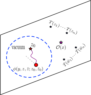
Figure 1: This figure suggests many aspects of our reconstruction strategy. We reconstruct a bulk operator $\phi$ connected by a Wilson line or ‘gravitational dressing’ that attaches to the boundary at $z_{0}$. Correlators of $\phi$ with stress tensors will only have singularities when the stress tensors approach $z_{0}$. When $\phi$ acts on the vacuum, it creates a state that we expand in radial quantization, and so when we define $\phi$ we assume it is surrounded by empty space. As our methods are ultimately based on symmetry, we only compute the proto-field $\phi$ as a linear combination of a CFT₂ primary ${\cal O}$ and its Virasoro descendants. All of these statements have analogs for the $U(1)$ charged $\phi$ we discuss as a warm-up in section 2, with $T\to J$.

We will be studying the terms in $\Phi$ involving ${\cal O}$ and any number of stress tensors, as these are determined by the Virasoro symmetry in AdS₃. Just as conformal symmetry dictates that CFT correlators must be decomposable as a sum of conformal blocks, bulk scalar fields $\Phi$ can be written as a sum of bulk proto-field operators $\phi$ that are fixed by symmetry.

The proto-fields $\phi$ also have another interpretation, as sources or sinks for one-particle states in a first-quantized worldline action description. Correlators of protofields $\langle\phi(X_{1})\phi(X_{2})\cdots\rangle$ with other CFT operators will match to all orders in perturbation theory with the propagation of a particle from $X_{1}$ to $X_{2}$ in the gravitational background created by these other CFT operators, including the effect of gravitational loops on the propagation. But the proto-field correlators do not include non-gravitational interactions, or mixings with multi-trace operators induced by gravity.

‘Dressings’ and Correlators with Symmetry Currents

Charged operators in gauge theories and local bulk operators in quantum gravity are not gauge-invariant. This means that their definition is ambiguous, and we need to supply more information to fully specify them. This additional information may be a Wilson line, a specific choice of gauge, or a ‘gravitational dressing’ (by this term we roughly mean ‘gravitational Wilson line’). We discuss the relation between these ideas in section 2.1.

The necessity and ambiguity of these dressings has a simple interpretation in the CFT. If we are to write a bulk proto-field $\phi(X)$ as a CFT operator, then the charge and energy in $\phi$ must be visible to the charge $Q$ and spacetime symmetries $D,P_{\mu},K_{\nu},M_{\mu\nu}$ in the CFT. These quantities can be computed by integrals of $J_{\mu}(x)$ or $T_{\mu\nu}(x)$ over Cauchy surfaces on the boundary Ginsparg , but the specific spacetime distribution of current and energy-momentum associated with $\phi(X)$ is somewhat arbitrary. This explains the ambiguity in $\phi(X)$, and also suggests how it can be fixed – the gauge and gravitational dressings are specified by the form of $\phi(X)$ correlators with $J_{\mu}(x)$ or $T_{\mu\nu}(x)$.

To make sense of this logic, it must be possible to distinguish the energy-momentum in $\phi(X)$ from that of other sources in any state or correlator. We accomplish this by assuming that $\phi(X)$ is surrounded by vacuum, so that we can define $\phi(X)$ in a series expansion in the bulk coordinate Paulos:2016fap , with local CFT operators as coefficients. In this way we can use radial quantization to define $\phi(X)$.

We will specify general gravitational dressings in two equivalent ways. In section 3.2 we use a trick: starting with the proto-field defined through Fefferman-Graham Anand:2017dav , we use a diffeomorphism to bend the gravitational dressing. Whereas in section 3.4 we take a more abstract route, and simply construct an operator $\phi(X;x_{0})$ at a point $X$ in the bulk, but where $T(x)$ on the boundary detects $\phi$’s associated stress-energy at a general point $x_{0}$.

Summary of Results

Our main result is a simple formula for a proto-field with general dressing

$$\phi\left(u,x,\bar{x};x_{0},\bar{x}_{0}\right)=\sum_{n=0}^{\infty}\sum_{m,\bar{m}=0}^{\infty}\frac{(-1)^{n}u^{2h+2n}}{n!(2h)_{n}}\frac{\left(x-x_{0}\right)^{m}\left(\bar{x}-\bar{x}_{0}\right)^{\bar{m}}}{m!\bar{m}!}\mathcal{L}_{-n-m}\bar{\mathcal{L}}_{-n-\bar{m}}\mathcal{O}(x_{0},\bar{x}_{0})$$ (1.3)

The interpretation of this operator is discussed in section 3, but roughly speaking, the proto-field is located $(u,x,\bar{x})$ in AdS₃, with its associated energy-momentum localized at $(x_{0},\bar{x}_{0})$ on the boundary. The ${\cal L}_{-N}$ are polynomials in the Virasoro generators determined by the bulk primary condition Anand:2017dav , with coefficients that are rational functions in the central charge $c$ and holomorphic dimension $h$ of ${\cal O}$. We verify that this result has the expected correlators with stress tensors $T(x)$. Our formula can be integrated against a positive, normalized distribution $\rho$ via

$$\phi[\rho](X)\equiv\int d^{2}x_{0}\,\rho(x_{0},\bar{x}_{0})\phi(X;x_{0},\bar{x}_{0})$$ (1.4)

to obtain a very general gravitational dressing for the proto-field.

We also show in section 4 that correlators of $\phi(X;x_{0},\bar{x}_{0})$ can be computed by a further adaptation Chen:2017dnl ; Chen:2018qzm of Zamolodchikov’s recursion relations ZamolodchikovRecursion ; Zamolodchikovq . Then in section 5 we analytically calculate the $1/c$ correction to the heavy-light, bulk-boundary propagator on the cylinder using a recent quantization Cotler:2018zff of AdS₃ gravity. We demonstrate that our analytic result matches that of the recursion relation. We also observe that as expected Fitzpatrick:2015dlt ; Fitzpatrick:2016ive , the analytic $1/c$ correction to the correlator is not periodic in Euclidean time Chen:2018qzm , and so it has a branch cut singularity at the Euclidean horizon. This is surprising from the point of view of perturbation theory in a fixed black hole background.

The outline of the paper is as follows. In section 2 we provide a detailed discussion of bulk reconstruction for fields charged under a $U(1)$ Chern-Simons field. This serves as a warm-up where many of the ideas can be more straightforwardly illustrated. Then in section 3 we turn to gravity, where many of our results are analogous to the simpler $U(1)$ setting. In section 4 we adapt a recursion relation to compute correlators of $\phi$ with general dressing. In section 5 we explain some rather technical calculations, including the recursion relation in a specific configuration and an analytic computation of the one-loop gravitational correction (i.e., order $1/c$) to a $\langle{\cal O}_{H}{\cal O}_{H}{\cal O}_{L}\phi_{L}\rangle$ correlator. We provide a brief discussion in section 6. Many technical results are relegated to the appendices.

2 Bulk Proto-Fields with $U(1)$ Chern-Simons Charge

This section will serve as a warm-up in preparation for our eventual discussion of bulk gravity, where most of these ingredients will have a direct analog.

2.1 Charged Fields, Wilson Lines, and Gauge Fixing

Consider a bulk field $\varphi(X)$ charged under a $U(1)$ gauge symmetry. It transforms as

$$\varphi(X)\to e^{iq\Lambda(X)}\varphi(X)$$ (2.1)

under the gauge redundancy, so it cannot be regarded as a physical observable. We can remedy this problem in two equivalent ways – by fixing the gauge, or by attaching $\varphi(X)$ to a Wilson line.

The latter approach has the clear advantage that it makes the gauge-invariant nature of our observable manifest. Given a Wilson line

$$W_{{\cal C}}(\infty,X)=e^{iq\int_{{\cal C}}dx^{\mu}A_{\mu}}$$ (2.2)

running from $X$ to infinity, we can form a non-local operator

$$\phi(X)=W_{{\cal C}}(\infty,X)\varphi(X)$$ (2.3)

Since gauge transformations do not act at infinity, $\phi$ will be a gauge-invariant observable. However, this means that $\varphi(X)$ itself was highly ambiguous, since $\phi$ now depends on the path of the Wilson line. Note that once we define a gauge-invariant $\phi$ in this way, we can compute observables involving it in any convenient gauge, and we will obtain the same results.

The other (fixing the gauge) approach will be easier to discuss when we generalize to quantum gravity. However, it’s less flexible and can lead to confusing terminology. In this approach we simply fix a gauge, for example by setting some component of the gauge field $A_{y}=0$, and then compute observables involving $\phi(X)$ in this gauge. The results will then be well-defined observables. Note that if $A_{y}=0$ then the Wilson line in the $\hat{y}$ direction $W_{\hat{y}}=1$ identically, so in this case the underlying gauge invariant observable will be $\phi=W_{\hat{y}}\varphi(X)$. But in general it may not be clear how to compute with our observable in other gauges. And it may seem confusing to refer to an observable defined in a specific gauge as gauge-invariant (though this is in fact true).

Let us develop these ideas in the context of a scalar field $\phi$ in AdS₃ charged under a $U(1)$ Chern-Simons theory with level $k$. The scalar will be dual to a CFT₂ primary operator ${\cal O}$ with conformal dimension $h$ and charge $q$, and the gauge field to a holomorphic conserved current $J(z)$. We will work in Euclidean space with a fixed metric

$$ds^{2}=\frac{dy^{2}+dzd\bar{z}}{y^{2}}$$ (2.4)

and in this section we will not include dynamical gravity.

We will be viewing $\phi(y,z,\bar{z})$ through the lens of radial quantization, as discussed previously in Anand:2017dav and pictured in figure 1 (the figure denotes the gravitational case, but with $T\to J$ it also applies to the present discussion). In the CFT $\phi$ will be a non-local operator, but only because it will be written as an infinite sum of local operators, each a coefficient in the near-boundary or small $y$ expansion of $\phi$. If we turn off both gravity and the Chern-Simons interaction, then $\phi$ is determined by symmetry to be Nakayama:2015mva

$$\phi_{0}(y,z,\bar{z})=\sum_{n=0}^{\infty}(-1)^{n}\frac{y^{2h+2n}}{n!(2h)_{n}}L_{-1}^{n}\bar{L}_{-1}^{n}{\cal O}(z,\bar{z})$$ (2.5)

This follows from the form of the vacuum bulk-boundary propagator

$$\langle\phi_{0}(y,z,\bar{z}){\cal O}^{\dagger}(w,\bar{w})\rangle=\left(\frac{y}{y^{2}+(z-w)(\bar{z}-\bar{w})}\right)^{2h}$$ (2.6)

if we expand in $y$ and identify the coefficients with global descendants of ${\cal O}$.

Now let us define a gauge-invariant charged scalar field. As discussed above, we can do this by simply attaching $\varphi$ to a Wilson line that ends on the boundary at $y=0$. A very simple choice takes the Wilson line to run in the $\hat{y}$ direction, so that

$$\phi(y,z,\bar{z})=e^{iq\int_{0}^{y}dy^{\prime}A_{y}(y^{\prime},z,\bar{z})}\varphi(y,z,\bar{z})$$ (2.7)

This operator also has a very simple definition via gauge fixing – it is simply $\phi$ defined in the gauge $A_{y}=0$. This makes it clear that the correlator $\langle\phi(y,0,0){\cal O}^{\dagger}(w,\bar{w})\rangle$ should be equal to the expression (2.6).

Correlators involving the boundary current will be non-trivial. Computing in perturbation theory gives

$$\langle J(z_{1}){\cal O}^{\dagger}(w,\bar{w})\phi(y,0,0)\rangle=\frac{qw}{z_{1}(z_{1}-w)}\left(\frac{y}{y^{2}+w\bar{w}}\right)^{2h},$$ (2.8)

where ${\cal O}^{\dagger}$ has charge $-q$. This reduces to $y^{2h}\langle J{\cal O}^{\dagger}{\cal O}\rangle$ in the limit of small $y$, as expected based on the AdS/CFT dictionary.

If we attach $\phi$ to the boundary with a more general Wilson line, then we will have

$$\phi(y,z,\bar{z};z_{0},\bar{z})=e^{iq\int_{z_{0}}^{X}dY^{\mu}A_{\mu}(Y)}\phi(y,z,\bar{z})$$ (2.9)

The Wilson line takes some general path from $z_{0}$ on the boundary to the location of $\phi$ in the bulk, yet our notation does not include information about the path. Since Chern-Simons theory is topological, our $\phi$ will only depend on this path if other charges or Wilson lines entangle with it. However, we are invoking radial quantization to define $\phi$, meaning that we will be assuming that there aren’t any matter fields or Wilson lines near $\phi$, or between it and the boundary. Thus our results for the operator $\phi$ will be independent of the choice of path, except through the location of $z_{0}$.

Correlators of this more general bulk field can still be computed in $A_{y}=0$ gauge. Since the vacuum equations of motion set $F_{y\mu}=0$, in this gauge $A_{z}$ is independent of $y$. Since on the boundary $A_{z}(0,z,\bar{z})=\frac{1}{k}J(z)$, this identification must hold for all $y$, so

$$\phi(y,z,\bar{z};z_{0},\bar{z})=\left.e^{i\frac{q}{k}\int_{z_{0}}^{z}J(z^{\prime})dz^{\prime}}\phi(y,z,\bar{z})\right|_{A_{y}=0}$$ (2.10)

This formula requires some regularization to remain consistent with ${\cal O}$ correlators and the dictionary ${\cal O}=\lim_{y\to 0}\left[y^{-2h}\phi\right]$. If we expand to first order in $q$ we find

$$\langle J(z_{1}){\cal O}^{\dagger}(w,\bar{w})\phi(y,0,0;z_{0},0)\rangle \approx\langle J(z_{1}){\cal O}^{\dagger}(w,\bar{w})\phi(y,0,0)\rangle+i\frac{q}{k}\int_{0}^{z_{0}}\langle J(z_{1}){\cal O}^{\dagger}(w,\bar{w})J(z^{\prime})\phi(y,0,\ 0)\rangle$$

$$\approx\frac{q(z_{0}-z)}{(z_{1}-z_{0})(z_{1}-z)}\langle{\cal O}^{\dagger}\phi\rangle$$ (2.11)

This formula has a nice interpretation, as the singularities in $z_{1}$ indicate the presence of charge $\pm q$ at $z_{0}$ and $z$. But higher order corrections involving many $J$ will produce divergent integrals. And even the simpler correlator $\langle{\cal O}^{\dagger}\phi\rangle$ also requires regularization.

In the next sections we will see how to avoid regularization by defining $\phi$ using symmetry when its Wilson line attachments are simple. Then we will extend our results to include general Wilson lines by leveraging the singularity structure of $\phi$ correlators.

2.2 A Bulk Primary Condition from Symmetry

We can take another approach, and constrain the bulk field $\phi$ using symmetry. If we can determine how to extend CFT symmetries into the bulk, then we can use their action on a charged bulk field to determine how to write it as a sum of CFT operators. This approach will provide an exact definition, without needing to regulate Wilson lines, and it will also generalize more directly to gravity.

The CFT current $J(z)$ can be expanded in modes

$$J\left(z\right)=\sum_{n=-\infty}^{\infty}\frac{J_{n}}{z^{n+1}}.$$ (2.12)

The global conformal generators have an algebra with $J_{n}$ with commutation relations

$$\left[L_{m},L_{n}\right] =\left(m-n\right)L_{m+n},$$

$$\left[L_{m},J_{n}\right] =-nJ_{n+m},$$ (2.13)

$$\left[J_{m},J_{n}\right] =mk\delta_{n+m,0},$$

where the subscripts of the $L$ generators runs from $-1$ to $1$, and the subscript of the $J$ generators run from $-\infty$ to $\infty$. The current acts on local primary operators via

$$[J_{n},{\cal O}(z)]=qz^{n}{\cal O}(z)$$ (2.14)

which can be derived from the $J(x){\cal O}(z)$ OPE. This means that a finite transformation $e^{i\delta J_{n}}$ will rephase ${\cal O}(z)\to e^{iq\delta z^{n}}{\cal O}(z)$.

Now we would like to understand how to extend these symmetries so that they act on bulk fields. This requires either a careful specification of the gauge invariant operators, or a choice of gauge. We will take the latter route and choose $A_{y}=0$. We can still transform $A_{z}\to A_{z}+\partial_{z}\lambda(z)$ while preserving this gauge fixing condition. But this is a global (rather than gauge) symmetry transformation, since it acts non-trivially on fields at the boundary $y=0$.

In the bulk, we expect that a charged field should transform as $\phi\to e^{i\lambda}\phi$. Since $\lambda$ cannot depend on $y$, this transforms $\phi(X)\to e^{i\lambda(z)}\phi(X)$. So in $A_{y}=0$ gauge, the $J_{n}$ act on $\phi$ in the same way that they act on ${\cal O}$, giving

$$\left.[J_{n},\phi(y,z,\bar{z})]=qz^{n}\phi(y,z,\bar{z})\right|_{A_{y}=0}$$ (2.15)

where we have indicated explicitly that this only holds in $A_{y}=0$ gauge. This further implies a bulk primary condition

$$[J_{n},\phi(y,0,0)]=0\ \ \ \mathrm{for}\ \ \ n\geq 1$$ (2.16)

for the bulk field $\phi$. This condition is the $U(1)$ Chern-Simons version of the gravitational bulk primary condition originally derived in Anand:2017dav . Along with the requirement that $\phi$ has the correct bulk-boundary propagator in vacuum (2.6), this bulk primary condition uniquely determines $\phi(y,z,\bar{z})$ as an expansion in $y$. Furthermore, it is an exact result, and does not require a small coupling expansion.

Notice that a gauge-invariant bulk operator $\phi(y,z,\bar{z})$ attached to the boundary by a Wilson line in the $\hat{y}$-direction must transform in the same way. This simply follows from the fact that $\phi=\varphi$ identically if the latter is defined in the gauge $A_{y}=0$.

We can write a formal solution to the bulk primary conditions as

$$\phi(y,z,\bar{z})=\sum_{n=0}^{\infty}\frac{(-1)^{n}}{n!(2h)_{n}}y^{2h+2n}{\cal J}_{-n}\bar{L}_{-1}^{n}{\cal O}\left(z,\bar{z}\right)$$ (2.17)

where ${\cal J}_{-n}{\cal O}$ is defined as an $n$th level descendant of ${\cal O}$ satisfying the bulk primary condition (2.16). In appendix B.1, we solve the the bulk primary condition exactly for the first several ${\cal J}_{-n}$s. As in section 3.2.2 of Anand:2017dav , it can be shown that ${\cal J}_{-n}$ can be written formally in terms of quasi-primaries as

$${\cal J}_{-n}{\cal O}=L_{-1}^{n}{\cal O}+n!\left(2h\right)_{n}\sum_{j=1}^{n}\sum_{i}\frac{L_{-1}^{n-j}{\cal O}_{h+j}^{\left(i\right)}}{\left|L_{-1}^{n-j}{\cal O}_{h+j}^{\left(i\right)}\right|^{2}}$$ (2.18)

where the ${\cal O}_{h+j}^{\left(i\right)}$ represent the $i$th quasi-primary at level $j$ (so they satisfy $L_{1}{\cal O}_{h+j}^{\left(i\right)}=0$) and the denominator is the norm of the corresponding operator. In writing down this equation, we’ve used the fact that the quasi-primaries can be chosen to be orthogonal to each other. This will be a very useful property for some of the discussions in the following sections. As a concrete example, ${\cal J}_{-1}$ is given by

$$\mathcal{J}_{-1}\mathcal{O}=L_{-1}\mathcal{O}+\frac{q^{2}}{2hk-q^{2}}\left(L_{-1}-\frac{2h}{q}J_{-1}\right)\mathcal{O}.$$ (2.19)

where the second term is a quasi-primary satisfying $L_{1}\left(L_{-1}-\frac{2h}{q}J_{-1}\right)\mathcal{O}=0$.

In appendix (B.2), we solve the bulk primary condition in the large $k$ limit for the all-order $\frac{1}{k}$ terms in ${\cal J}_{-n}$. As shown in both appendix (B.1) and (B.2), in the $k\to\infty$, we have ${\cal J}_{-n}=L_{-1}^{n}+O(1/k)$, so our expansion in $y$ reduces to that of equation (2.5). Note that as in Anand:2017dav , $\phi$ is a non-local operator in the CFT due to the infinite sum in its definition.

Since the bulk proto-field has been defined as an expansion in descendants of a local CFT primary, we will often informally discuss the ‘OPE’ of the current $J$ with $\phi$. Because of the bulk primary condition above, the singular term in the OPE of $J\left(z_{1}\right)$ and $\phi\left(y,z,z\right)$ is very similar to the $J{\cal O}$ OPE (which is simply $J(z_{1}){\cal O}(z,\bar{z})\sim\frac{q{\cal O}(z,\bar{z})}{z_{1}-z}+\cdots$):

$$J\left(z_{1}\right)\phi\left(y,z,\bar{z}\right)\sim\frac{q\phi\left(y,z,\bar{z}\right)}{z_{1}-z}+\cdots$$ (2.20)

where we have used $[J_{0},\phi]=q\phi$, since the descendant operators in $\phi$ all have the same charge $q$.

Using these CFT definitions of the bulk charged scalar $\phi$, we can compute various correlation functions, such as $\left\langle\phi{\cal O}^{\dagger}J\cdots J\right\rangle$ and $\left\langle\phi^{\dagger}\phi\right\rangle$. We can first verify that $\phi$ given in (2.17) indeed gives the correct bulk-boundary propagator. Using (2.18), one can see $\langle\phi{\cal O}^{\dagger}\rangle$ is given by

$$\left\langle\phi\left(y,z,z\right){\cal O}^{\dagger}\left(w,\bar{w}\right)\right\rangle=\left(\frac{y}{y^{2}+(z-w)(\bar{z}-\bar{w})}\right)^{2h}.$$ (2.21)

simply because the quasi-primary terms in ${\cal J}_{-n}{\cal O}$ do not contribute to this two-point function and the calculation reduces to that of $\langle\phi_{0}{\cal O}^{\dagger}\rangle$ with $\phi_{0}$ given by (2.5). The bulk-boundary three-point function $\langle JO^{\dagger}\phi\rangle$ can be computed simply using the OPE of $J{\cal O}^{\dagger}$ and $J\phi$ (equation (2.20)), and the result is given by

$$\left\langle J\left(z_{1}\right){\cal O}^{\dagger}\left(w,\bar{w}\right)\phi\left(y,z,z\right)\right\rangle=q\left(\frac{1}{z_{1}-z}-\frac{1}{z_{1}-w}\right)\left\langle\phi\left(y,z,z\right){\cal O}^{\dagger}\left(w,\bar{w}\right)\right\rangle.$$ (2.22)

Correlation functions of the form $\left\langle\phi{\cal O}^{\dagger}J\cdots J\right\rangle$ can then be computed recursively using OPEs used above and the $JJ$ OPE.

For the bulk two-point function $\left\langle\phi^{\dagger}\phi\right\rangle$, we compute up to order $1/k$ using the perturbative approximation to $\phi$ that we derived in appendix (B.2), which corresponds to the one photon-loop correction to the bulk propagator. The details of the calculation are given in appendix C.1. The result for $\left\langle\phi^{\dagger}\left(y_{1},z_{1},\bar{z}_{1}\right)\phi\left(y_{2},\bar{z}_{2},\bar{z}_{2}\right)\right\rangle$ is given by

$$\left\langle\phi^{\dagger}\phi\right\rangle=\frac{\rho^{h}}{1-\rho}\left[1-\frac{q^{2}}{k}\left(\frac{\rho_{2}^{2}F_{1}(1,2h+1;2(h+1);\rho)}{2h+1}+\frac{\rho}{2h}-\log(1-\rho)\right)\right]+O\left(\frac{1}{k^{2}}\right)$$ (2.23)

where $\rho=\left(\frac{\xi}{1+\sqrt{1-\xi^{2}}}\right)^{2}$ with $\xi=\frac{2y_{1}y_{2}}{y_{1}^{2}+y_{2}^{2}+z_{12}\bar{z}_{12}}$.

In appendix C we also use the bulk Witten diagrams to compute $\left\langle J{\cal O}^{\dagger}\phi\right\rangle$ and $\left\langle\phi^{\dagger}\phi\right\rangle$, and the results exactly match equations (2.22) and (2.23). This provides a non-trivial check of our definition of a charged bulk scalar field.

2.3 Singularities in $J(z)$ and the AdS Equations of Motion

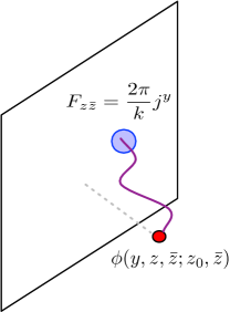
Figure 2: This figure indicates the relationship between singularities in the current $J(z)$, the bulk equations of motion, and Wilson lines. Analogous statements hold for gravity and connect singularities in $T(z)$ to the gravitational dressing.

The singularity structure of the $J(z)$ correlators in equation (2.22) follow from the bulk equations of motion. So these singularities indicate the placement of Wilson lines attaching bulk charges to the boundary, and vice versa. Let us briefly explain these statements, which are illustrated in figure 2.

In the $U(1)$ Chern-Simons theory, the equations of motion are

$$\epsilon^{abc}F_{bc}(X)=\frac{2\pi}{k}j^{a}(X)$$ (2.24)

for the bulk matter charge $j^{a}(X)$ and bulk field strength $F_{ab}$. In the presence of a Wilson line with components in the $\hat{y}$ direction, $j^{y}$ will receive a delta function contribution localized to the Wilson line. This means that $F_{z\bar{z}}$ must include a delta function. In $A_{y}=0$ gauge, we can identify $A_{z}(y,z,\bar{z})=\frac{1}{k}J(z)$, so

$$\partial_{\bar{z}}J(z)=2\pi q\,\delta^{2}(z,\bar{z})$$ (2.25)

or equivalently

$$\oint dzJ(z)=2\pi iq$$ (2.26)

To satisfy this constraint, the current must have a simple pole $J(z)=\frac{q}{z}+\cdots$, where the ellipsis denotes less singular terms as $z\to 0$. So the singularity structure of correlators with $J(z)$ follows directly from the bulk equations of motion. Conversely, a singularity in $J(z)$ in correlators with other operators indicates the presence of charge.

This means that we can use the singularity structure of correlators with $J(z)$ or $T(z)$ in the case of gravity to help to define a bulk field $\phi$ with a more general Wilson line attachment or ‘gravitational dressing’. Similar observations also hold in higher dimensions, and may be useful for bulk reconstruction more generally.

2.4 Charged Bulk Operators and General Wilson Lines

In section 2.2 we constructed a charged bulk scalar field by fixing to the gauge $A_{y}=0$. In so doing we defined a gauge-invariant bulk field $\phi(y,z,\bar{z})$ connected to the boundary by a Wilson line in the $\hat{y}$ direction. In this section, we are going to construct an exact gauge-invariant bulk field whose associated Wilson line attaches to an arbitrary point $z_{0}$ on the boundary.

There are several ways to approach the construction of this general $\phi(y,z,\bar{z};z_{0},\bar{z})$. The most immediate one was already discussed in section 2.1, namely including an explicit Wilson line. An issue with this approach is that it requires a regulator for divergences in intermediate calculations, and this makes it difficult to define $\phi$ non-perturbatively. Another important limitation is that it’s challenging to work with Wilson lines for bulk diffeomorphisms, as would be necessary when we turn to gravity.

Instead of inserting an explicit Wilson line, we can define $\phi$ using the singularity structure of current correlators. Correlators involving $J(z_{1})$ and the field $\phi(y,z,\bar{z})$ defined in $A_{y}=0$ gauge have singularities as $z_{1}\to z$. These singularities represent the charge of the bulk $\phi$ on the boundary, as emphasized in section 2.3. If a Wilson line connects $\phi$ to the boundary at $z_{0}$, then instead we expect that correlators involving $J(z_{1})\phi$ will have singularities at $z_{0}$.

Thus we need a way to move the singularities in $z_{1}$ for all correlators involving $J(z_{1})$ and $\phi$. In fact, we already have many of the technical tools that we need. The level $n$ descendants ${\cal J}_{-n}{\cal O}$ defined in section 2.2 were constructed so that they would not have any additional singularities in the $J(z_{1}){\cal J}_{-n}{\cal O}$ OPE beyond those already present in $J(z_{1}){\cal O}$. We can use these ${\cal J}_{-n}$ to move an operator without moving the singularities associated with its charge (we develop this idea in more detail in appendix A). The point is that since ${\cal J}_{-n}=L_{-1}^{n}+\cdots$ as shown in equation (2.18), we have that

$$\sum_{n=0}^{\infty}\frac{x^{n}}{n!}{\cal J}_{-n}=e^{xL_{-1}}+\cdots$$ (2.27)

where the ellipsis denotes terms proportional to powers of the charge $q$. So this expression acts like a combination of a translation and a $U(1)$ symmetry transformation. This means that the non-local operator

$$\tilde{{\cal O}}\left(z,\bar{z};z_{0},\bar{z}\right)=\sum_{n=0}^{\infty}\frac{\left(z-z_{0}\right)^{n}}{n!}{\cal J}_{-n}{\cal O}\left(z_{0},\bar{z}\right).$$ (2.28)

behaves like a kind of mirage. It is defined so that $J\left(z_{1}\right)\tilde{{\cal O}}\left(z,\bar{z};z_{0},\bar{z}\right)$ only has singularities in $z_{1}-z_{0}$, while correlators of $\tilde{{\cal O}}\left(z,\bar{z};z_{0},\bar{z}\right)$ with ${\cal O}^{\dagger}\left(w,\bar{w}\right)$ will instead have singularities when $w-z$ vanishes. Explicitly, by using the OPEs of ${\cal J}{\cal O}^{\dagger}$ and ${\cal J}\tilde{\cal O}$ and properties of ${\cal J}_{-n}$, we have

$$\langle J(z_{1}){\cal O}^{\dagger}(w,\bar{w})\tilde{\cal O}(z,\bar{z};z_{0},\bar{z})\rangle=\frac{q(z_{0}-w)}{(z_{1}-z_{0})(z_{1}-w)}\frac{1}{(z-w)^{2h}(\bar{z}-\bar{w})^{2\bar{h}}}$$ (2.29)

so $\tilde{\cal O}(z,\bar{z};z_{0},\bar{z})$ behaves as though it is in two places at once.

We can generalize the above idea to obtain a bulk proto-field $\phi\left(y_{1},z,\bar{z};z_{0},\bar{z}\right)$ at $\left(y,z,\bar{z}\right)$ with a Wilson line landing at $\left(z_{0},\bar{z}\right)$ on the boundary. This leads to a proposal for a charged bulk field with a more general Wilson line attachment

$$\phi\left(y,z,\bar{z};z_{0},\bar{z}\right)=\sum_{n=0}^{\infty}\sum_{m=0}^{\infty}(-1)^{n}\frac{y^{2h+2n}}{n!(2h)_{n}}\frac{(z-z_{0})^{m}}{m!}\mathcal{J}_{-n-m}\bar{L}_{-1}^{n}\mathcal{O}\left(z_{0},\bar{z}\right),$$ (2.30)

In fact, this form for $\phi$ is uniquely fixed by demanding that:

1. $\langle\phi{\cal O}^{\dagger}\rangle$ takes the vacuum form given in equation (2.6)

2. Correlators $\langle{\cal O}^{\dagger}(w,\bar{w})J(z_{1})\cdots J(z_{n})\phi(y,z,\bar{z};z_{0},\bar{z})\rangle$ only have simple poles in the $z_{i}$, which can only occur when $z_{i}\to z_{0}$ or $z_{i}\to w$.

Note that if $z=z_{0}$, then only the $m=0$ terms contribute to equation (2.30), and $\phi$ reduces to the bulk field of equation (2.17). To obtain ${\cal O}(z,\bar{z})$ as we take $y\to 0$, we need to simultaneously send $z_{0}\to z$; otherwise we obtain the non-local operator $\tilde{\cal O}(z,\bar{z};z_{0},\bar{z})$ of equation (2.28).

We can verify that $\phi\left(y,z,\bar{z};z_{0},\bar{z}\right)$ is really the desired operator by computing $\left\langle{\cal O}^{\dagger}\phi\right\rangle$ and $\left\langle J{\cal O}^{\dagger}\phi\right\rangle$ using the properties of ${\cal J}_{-n}$s. For the bulk-boundary propagator $\left\langle{\cal O}^{\dagger}\left(w,\bar{w}\right)\phi\left(y,z,\bar{z};z_{0},\bar{z}\right)\right\rangle$, since the quasi-primaries terms in ${\cal J}_{-n}{\cal O}$ (equation (2.18)) will not contribute, we can simply replace ${\cal J}_{-n}{\cal O}$ with $L_{-1}^{n}{\cal O}$. But then the sum over $m$ becomes exactly a translation operator, and the $\phi$ in (2.30) becomes the free-field $\phi_{0}$ of (2.5), and we have

$$\left\langle{\cal O}^{\dagger}\left(w,\bar{w}\right)\phi\left(y,z,\bar{z};z_{0},\bar{z}\right)\right\rangle=\left\langle{\cal O}^{\dagger}\left(w,\bar{w}\right)\phi_{0}\left(y,z,\bar{z}\right)\right\rangle=\left(\frac{y}{y^{2}+\left(z-w\right)\left(\bar{z}-\bar{w}\right)}\right)^{2h},$$ (2.31)

as expected. For $\left\langle J{\cal O}^{\dagger}\phi\right\rangle$, we can use the OPEs $J\left(z_{1}\right){\cal O}^{\dagger}\left(w,\bar{w}\right)\sim\frac{-q{\cal O}^{\dagger}\left(w,\bar{w}\right)}{z_{1}-w}+\cdots$ and $J\left(z_{1}\right)\phi\left(y,z,\bar{z};z_{0},\bar{z}\right)\sim\frac{q}{z_{1}-z_{0}}\phi\left(y,z,\bar{z};z_{0},\bar{z}\right)+\cdots$, where the ellipses denotes non-singular terms. $\left\langle J{\cal O}^{\dagger}\phi\right\rangle$ can then be computed by only including the singular terms in both OPEs, and we get

$$\left\langle J\left(z_{1}\right){\cal O}^{\dagger}\left(w,\bar{w}\right)\phi\left(y,z,\bar{z};z_{0},\bar{z}\right)\right\rangle=q\frac{z_{0}-w}{\left(z_{1}-z_{0}\right)\left(z_{1}-w\right)}\left(\frac{y}{y^{2}+\left(z-w\right)\left(\bar{z}-\bar{w}\right)}\right)^{2h}.$$ (2.32)

Note that here the singularities are at $z_{1}=w$ and $z_{1}=z_{0}$, while in equation (2.22), the singularities were at $z_{1}=w$ and $z_{1}=z$.

Before concluding this section, we should emphasize that our methods are insensitive to the trajectory that the Wilson line takes from $(y,z,\bar{z})$ in the bulk to the boundary point $z_{0}$. This is possible because the bulk theory is topological, and we have assumed that $\phi$ is surrounded by a region of vacuum, so that it’s possible to define $\phi$ in radial quantization. Our gravitational $\phi$ will be defined in the same way.

2.5 More General Bulk Operators from Sums of Wilson Lines

In prior sections we have developed a formalism for exactly defining and evaluating an operator $\phi(X;z_{0})$, where a Wilson line connects $X\equiv(y,z,\bar{z})$ to a point $z_{0}$ on the boundary. But there are a host of other choices for gauge-invariant bulk operators. We can explore this space by defining a new bulk operator

$$\phi[\rho](X)\equiv\int d^{2}z_{0}\,\rho(z_{0},\bar{z}_{0})\phi(X;z_{0},\bar{z})$$ (2.33)

where $\rho(z_{0},\bar{z}_{0})>0$ and $\int d^{2}z_{0}\rho(z_{0},\bar{z}_{0})=1$. The properties of $\phi[\rho]$ are inherited from $\phi(X;z_{0})$, which is simply the special case where $\rho(x)=\delta(x-z_{0})$. Note that if we like, we can let $\rho$ depends on $X$ so that $\rho$ varies as we move $\phi$ to different locations $X$ in the bulk.

Operators like $\phi[\rho]$ make it possible to study bulk fields with far more general ‘dressings’, which include superpositions of Wilson lines. For example, we might define a bulk field with spherically symmetric dressing. Let the bulk field be located at the point $(y,z,\bar{z})$ in Poincare patch and $(t_{E},r,\theta)$ in global coordinates, and let the point of attachment of the Wilson line to the boundary be $z_{0}$. We will average with the measure $\frac{d\theta}{2\pi}$ over the spatial circle on the boundary at fixed $t_{E}$. In Poincare patch this means integrating with the measure $\frac{dz_{0}}{2\pi iz_{0}}$ along the contour $|z_{0}|=|z|\sqrt{1+\frac{y^{2}}{z\bar{z}}}$. The integration contour ensures that $z_{0}$ is on the same time slice as the bulk field. In summary, the integration measure is

$$\rho(z_{0},\bar{z}_{0})=\frac{1}{2\pi iz_{0}}\delta\left(|z_{0}|-|z|\sqrt{1+\frac{y^{2}}{z\bar{z}}}\right)$$ (2.35)

Note that $\int d^{2}z_{0}\rho(z_{0},\bar{z}_{0})=1$. The integration of $\langle J\mathcal{O}^{\dagger}\phi\rangle$ (equation 2.32) then gives

$$\frac{\langle J(z_{1})\mathcal{O}^{\dagger}(w,\bar{w})\phi[\rho](y,z,\bar{z})\rangle}{\langle\phi(y,z,\bar{z}){\cal O}(w,\bar{w})\rangle} =q\left(\frac{\Theta(|z_{1}|-|z_{0}|)}{z_{1}}-\frac{1}{z_{1}-w}\right)$$ (2.36)

where $|z_{0}|$ denotes $|z|\sqrt{1+\frac{y^{2}}{z\bar{z}}}$ and $\Theta$ is the Heaviside step function. Since $J_{0}=\frac{1}{2\pi i}\oint dz_{1}J(z_{1})$, we can further contour integrate the above expression with respect to $z_{1}$ to obtain the total charge of the state. The result is given by

$$q\left(\Theta(|z_{1}|-|z_{0}|)-\Theta(|z_{1}|-|w|)\right)$$ (2.37)

The interpretaton of this is clear: A state created by $\phi$ or $\mathcal{O}^{\dagger}$ carries charges $q$ and $-q$ respectively, and the charge content of the state at the time of insertion of $J$ depends upon the insertions that occur before that time. This result should be equivalent to Coulomb gauge Dirac:1955uv to lowest order in perturbation theory, but will not agree more generally, because the exponential of an average is not equal to the average of an exponential.

3 Gravitational Proto-Fields with General Dressing

There are no local gauge invariant operators in gravity. To understand this, observe that diffeomorphism gauge redundancies act on local scalar fields via

$$\varphi(x)\to\varphi(x)+\xi^{\mu}(x)\nabla_{\mu}\varphi(x)$$ (3.1)

This is similar to $U(1)$ gauge theory, where a charged field transforms as $\varphi\to\varphi+iq\Lambda(x)\varphi$, insofar as in both cases, local fields by themselves are not gauge-invariant. As we discussed in detail in section 2, we can form gauge invariant quasi-local charged operators in a $U(1)$ theory using Wilson line attachments.

Matters are not so simple in the case of gravity, because it is the dependence of $\varphi$ on the bulk coordinates themselves that renders $\varphi$ gauge non-invariant. Lacking a simple and general notion of a gravitational Wilson line, we will discuss diffeomorphism gauge-invariant operators as ‘gravitationally dressed’ local operators. In this section, we consider gravitational dressings that associate local bulk operators with specific points on the boundary. Such dressings are natural analogs of Wilson lines joining a field in the bulk to a point on the boundary.

We will use the notation $\phi(y,z,\bar{z};z_{0},\bar{z}_{0})$ to denote a diffeomorphism invariant bulk proto-field at $(y,z,\bar{z})$ in AdS₃ that has a gravitational line dressing landing on the boundary at the point $(z_{0},\bar{z}_{0})$. The simplified notation $\phi(y,z,\bar{z})$ is used when the boundary point of the gravitational dressing is at $(z,\bar{z})$. We sometimes refer to the path that the associated gravitational dressing takes, but strictly speaking our results are not associated with any particular path. In our formalism all paths are equivalent because we assume that the bulk field can be connected to the boundary through the bulk vacuum.

Our typical setup is pictured in figure 1. Some of our analysis will be analogous to the simpler and conceptually clearer $U(1)$ Chern-Simons case discussed in section 2. However, we will provide more details about the relationship between diffeomorphisms and gravitational dressing, and explain how some simple correlation functions can be computed.

3.1 Review of Protofields in Fefferman-Graham Gauge

In recent work Anand:2017dav ; Chen:2017dnl ; Chen:2018qzm , an exact gravitational proto-field was defined with a very specific gravitational dressing. The dressing was determined implicitly, by fixing to a Fefferman-Graham or Banados gauge Banados:1998gg where the metric takes the form

$$d\hat{s}^{2}=\frac{dy^{2}+dzd\bar{z}}{y^{2}}-\frac{6T(z)}{c}dz^{2}-\frac{6\bar{T}(\bar{z})}{c}d\bar{z}^{2}+y^{2}\frac{36T(z)\bar{T}(\bar{z})}{c^{2}}dzd\bar{z}.$$ (3.2)

Away from sources of bulk energy, $d\hat{s}^{2}$ may be viewed as an operator whose VEV corresponds to the semiclassical metric. That is, for a CFT state $|\psi\rangle$, the semiclassical metric will be given by $ds_{|\psi\rangle}^{2}=\langle\psi|d\hat{s}|\psi\rangle$, which is the RHS of the above equation with $T(z)\rightarrow\langle\psi|T(z)|\psi\rangle$ and $\bar{T}(z)\rightarrow\langle\psi|\bar{T}(z)|\psi\rangle$. In this subsection, we are considering the case where the CFT is living on a flat Euclidean plane with coordinates $(z,\bar{z})$. So for the CFT vacuum $|0\rangle$, we have $\langle 0|T(z)|0\rangle=0$ and $\langle 0|\bar{T}(z)|0\rangle=0$, and the bulk metric is the Poincare metric $ds_{|0\rangle}^{2}=\frac{dy^{2}+dzd\bar{z}}{y^{2}}$.

Once we gauge fix, Virasoro symmetry transformations extend to a unique set of vector fields in the bulk. Demanding that $\phi(y,z,\bar{z})$ transforms as a scalar field under the corresponding infinitesimal diffeomorphisms then implies that it must satisfy the bulk primary conditions Anand:2017dav

$$[L_{n},\phi(y,0,0)]=0,\quad[\bar{L}_{n},\phi(y,0,0)]=0,\quad n\geq 2,$$ (3.3)

along with the condition that in the vacuum $ds_{|0\rangle}^{2}=\frac{dy^{2}+dzd\bar{z}}{y^{2}}$, the bulk-boundary propagator is

$$\langle\mathcal{O}(z,\bar{z})\phi(y,0,0)\rangle=\frac{y^{2h_{L}}}{\left(y^{2}+z\bar{z}\right)^{2h_{L}}}.$$ (3.4)

These conditions uniquely determine $\phi(y,0,0)$ as a CFT operator defined by its series expansion in the radial $y$ coordinate:

$$\phi(y,0,0)=y^{2h_{L}}\sum_{N=0}^{\infty}\frac{(-1)^{N}y^{2N}}{N!\left(2h_{L}\right)_{N}}\mathcal{L}_{-N}\bar{\mathcal{L}}_{-N}\mathcal{O}(0).$$ (3.5)

This is a bulk proto-field in the metric of equation (3.2). The $\mathcal{L}_{-N}$ are polynomials in the Virasoro generators at level $N$, with coefficients that are rational functions of the dimension $h$ of the scalar operator ${\cal O}$ and of the central charge $c$. They are obtained by solving the bulk-primary conditions (3.3) exactly (no large $c$ expansion is required). And as shown in section 3.2.2 of Anand:2017dav , they can be written formally in terms of quasi-primaries as

$$\mathcal{L}_{-N}\mathcal{O}=L_{-1}^{N}{\cal O}+N!(2h)_{N}\sum_{n=2}^{N}\sum_{i}\frac{L_{-1}^{N-n}\mathcal{O}_{h+n}^{(i)}}{\left|L_{-1}^{N-n}\mathcal{O}_{h+n}^{(i)}\right|^{2}}$$ (3.7)

where $\mathcal{O}_{h+n}^{(i)}$ is the $i$th quasi-primary at level $n$ and the denominator is the norm of the corresponding operator. In writing this equation, we have used the fact that the quasi-primaries can be chosen so that they are orthogonal to each other. This will be a very useful property of ${\cal L}_{-N}{\cal O}$ in later discussions.

The correlation function $\langle\phi{\cal O}T\rangle$ was computed and it was found that Anand:2017dav

$$\frac{\left\langle\phi(y,0,0)\mathcal{O}(z,\bar{z})T\left(z_{1}\right)\right\rangle}{\langle\phi(y,0,0)\mathcal{O}(z,\bar{z})\rangle}=\frac{hz^{2}}{z_{1}^{3}\left(z_{1}-z\right)^{2}}\left(z_{1}+\frac{2y^{2}\left(z_{1}-z\right)}{y^{2}+z\bar{z}}\right).$$ (3.8)

Notice that this correlator has a cubic singularity when the position $z_{1}$ of the energy-momentum tensor $T$ approaches the point $(0,0)$. Roughly speaking, this singularity is the boundary imprint of the energy-momentum of the bulk field. It demonstrates the presence of a gravitational dressing connecting $\phi$ to the boundary point $(0,0)$. The boundary energy-momentum tensor $T(z_{1})$ can detect this dressing via the cubic singularity, just as the current $J(z_{1})$ registered the charge of a bulk field by a similar, but lower-order, singularity, as discussed in section 2.3. On a more formal level, contour integrals $\oint z_{1}^{2+n}T(z_{1})$ surrounding the singularity pick out the action of conformal generators $L_{n}$ on the bulk field $\phi$.

Using our more general notation $\phi(y,z,\bar{z};z_{0},\bar{z}_{0})$, the proto-field $\phi(y,0,0)$ given in equation (3.5) is the gauge-invariant operator $\phi(y,0,0;0,0)$ evaluated in the Fefferman-Graham gauge. The gravitational dressing is in the $\hat{y}$ direction. In the next subsection, we are going to construct bulk proto-fields that have more general dressings.

3.2 Natural Gravitational Dressings from Diffeomorphisms

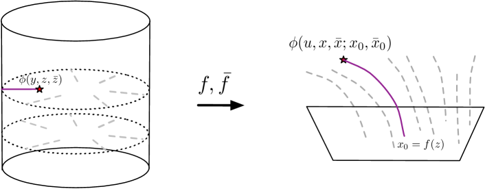
Figure 3: This figure suggests the use of a diffeomorphism to generate a natural gravitational dressing for a CFT living on a curved space, such as the cylinder. A curved dressing in the $(u,x,\bar{x})$ coordinates, with the CFT living on a plane, is mapped using equation (3.2) to a radial dressing in global AdS and BTZ black hole backgrounds.

In many situations it is convenient to place the CFT on a two-dimensional surface other than the plane. For example, in the presence of a BTZ black hole it’s more natural to place the CFT on a cylinder, as will be discussed in section 5. In this section we will demonstrate how to define scalar proto-fields with a correspondingly natural dressing, greatly generalizing the results of section 3.1. The ideas are illustrated in figure 3.

General vacuum AdS₃ metrics with different boundary geometries can be obtained from the CFT on a plane

$$ds^{2}=\frac{du^{2}+dxd\bar{x}}{u^{2}}$$ (3.9)

by the following coordinate transformation Roberts:2012aq

$$u =y\frac{4\left(f^{\prime}(z)\bar{f}^{\prime}(\bar{z})\right)^{\frac{3}{2}}}{4f^{\prime}(z)\bar{f}^{\prime}(\bar{z})+y^{2}f^{\prime\prime}(z)\bar{f}^{\prime\prime}(\bar{z})}$$

$$x =f(z)-\frac{2y^{2}\left(f^{\prime}(z)\right)^{2}\bar{f}^{\prime\prime}(\bar{z})}{4f^{\prime}(z)\bar{f}^{\prime}(\bar{z})+y^{2}f^{\prime\prime}({z})\bar{f}^{\prime\prime}(\bar{z})}$$ (3.10)

$$\bar{x} =\bar{f}(\bar{z})-\frac{2y^{2}\left(\bar{f}^{\prime}(\bar{z})\right)^{2}f^{\prime\prime}(z)}{4f^{\prime}(z)\bar{f}^{\prime}(\bar{z})+y^{2}f^{\prime\prime}(z)\bar{f}^{\prime\prime}(\bar{z})}.$$

The resulting vacuum AdS₃ metric is then given by

$$ds^{2}=\frac{dy^{2}+dzd\bar{z}}{y^{2}}-\frac{1}{2}S_{f}(z)dz^{2}-\frac{1}{2}\bar{S}_{\bar{f}}(\bar{z})d\bar{z}^{2}+y^{2}\frac{S_{f}(z)\bar{S}_{\bar{f}}(\bar{z})}{4}dzd\bar{z}.$$ (3.11)

where $S_{f}(z)\equiv\frac{f^{\prime\prime\prime}(z)}{f^{\prime}(z)}-\frac{3}{2}\left(\frac{f^{\prime\prime}(z)}{f^{\prime}(z)}\right)^{2}$ is the Schwarzian derivative.

In this section, we would like to obtain a formula for a bulk proto-field $\phi(y,z,\bar{z})$ with a gravitational dressing in the $\hat{y}$ direction. The difference between this section and section 3.1 is that in this section, the CFT is living on a different 2d surface. This may seem confusing, since the boundary here is also described by $(z,\bar{z})$, but here the energy-momentum tensor has a non-vanishing VEV given by $\langle 0|T(z)|0\rangle=\frac{c}{12}S_{f}$. For example, if $f(z)=e^{z}$ and $\bar{f}(\bar{z})=e^{\bar{z}}$ (see Section 3.3.2 for more details about this example), then ($z,\bar{z}$) are naturally coordinates on a cylinder and $S_{f}=-\frac{1}{2}$ (i.e. $\langle 0|T(z)|0\rangle=-\frac{c}{24}$, which is the expectation value of the energy-momentum tensor on the cylinder). In other words, the metric dual to the CFT vacuum $|0\rangle$ here is given by (3.11) with a $S_{f}\neq 0$, whereas in section 3.1 the metric dual to the CFT vacuum is given by the Poincare metric $ds^{2}=\frac{dy^{2}+dzd\bar{z}}{y^{2}}$ with planar boundary.

To obtain a bulk proto-field operator $\phi(y,z,\bar{z})$ with a gravitational dressing in the $\hat{y}$ direction, we can consider what this operator corresponds to in the $(u,x,\bar{x})$ coordinates of equation (3.9). The position $(y,z,\bar{z})$ of this operator will be mapped to $(u(y,z,\bar{z}),x(y,z,\bar{z}),\bar{x}(y,z,\bar{z}))$, and the boundary point of the gravitational dressing $(y=0,z,\bar{z})$ will be mapped to the boundary point $(u=0,x_{0}=f(z),\bar{x}_{0}=\bar{f}(\bar{z})$). Therefore we can also denote the operator $\phi(y,z,\bar{z})$ as follows

$$\phi(y,z,\bar{z})\equiv\phi(u,x,\bar{x};x_{0},\bar{x}_{0})$$ (3.12)

with the understanding that $(u,x,\bar{x})$ are functions of $(y,z,\bar{z})$ as given by (3.11) and $x_{0}=f(z)$ and $\bar{x}_{0}=\bar{f}(\bar{z})$. Although in the $(y,z,\bar{z})$ coordinates, the gravitational dressing is in the $\hat{y}$ direction, in the $(u,x,\bar{x})$ coordinates the dressing is not in the $\hat{u}$ direction, since typically $x_{0}\neq x$ and $\bar{x}_{0}\neq\bar{x}$.

These observations imply that in the $(u,x,\bar{x})$ coordinates, the bulk-boundary propagator should be given by

$$\left\langle\phi\left(u,x,\bar{x};x_{0},\bar{x}_{0}\right)\mathcal{O}\left(x_{1},\bar{x}_{1}\right)\right\rangle=\left(\frac{u}{u^{2}+\left(x-x_{1}\right)\left(\bar{x}-\bar{x}_{1}\right)}\right)^{2h}.$$ (3.13)

The new operator must also satisfy the bulk-primary conditions

$$[L_{n}^{\left(x_{0}\right)},\phi\left(u,x,\bar{x};x_{0},\bar{x}_{0}\right)]=0,\quad[\bar{L}_{n}^{\left(\bar{x}_{0}\right)},\phi\left(u,x,\bar{x};x_{0},\bar{x}_{0}\right)]=0,\quad n\geq 2$$ (3.14)

The above two conditions uniquely fix $\phi\left(u,x,\bar{x};x_{0},\bar{x}_{0}\right)$ to be

$$\phi\left(u,x,\bar{x};x_{0},\bar{x}_{0}\right)=\sum_{n=0}^{\infty}\sum_{m,\bar{m}=0}^{\infty}\frac{(-1)^{n}u^{2h+2n}}{n!(2h)_{n}}\frac{\left(x-x_{0}\right)^{m}\left(\bar{x}-\bar{x}_{0}\right)^{\bar{m}}}{m!\bar{m}!}\mathcal{L}_{-n-m}\bar{\mathcal{L}}_{-n-\bar{m}}\mathcal{O}\left(x_{0},\bar{x}_{0}\right).$$ (3.16)

Note that the $\mathcal{L}_{-n-m}$ and $\bar{\mathcal{L}}_{-n-\bar{m}}$ here are defined on the boundary complex plane $(x,\bar{x})$, where $T(x),\bar{T}(\bar{x})$ are quantized by expanding around the point $(x_{0},\bar{x}_{0})$. It’s obvious that the above equation satisfies the bulk-primary conditions (3.14), since the ${\cal L}_{-N}$s and $\bar{{\cal L}}_{-\bar{N}}$s are constructed as solutions to such conditions. Using the property (3.7) of the ${\cal L}_{-N}$s, it’s easy to see why $\phi\left(u,x,\bar{x};x_{0},\bar{x}_{0}\right)$ has the correct bulk-boundary propagator (3.13) with ${\cal O}(x_{1},\bar{x}_{1})$, since the quasi-primary terms in $\mathcal{L}_{-n-m}\bar{\mathcal{L}}_{-n-\bar{m}}\mathcal{O}$ will not contribute in this two-point function. So when computing (3.13), we can simply replace the $\mathcal{L}_{-n-m}\bar{\mathcal{L}}_{-n-\bar{m}}\mathcal{O}$ with $L_{-1}^{n+m}\bar{L}_{-1}^{n+\bar{m}}{\cal O}$, and the sums over $m$ and $\bar{m}$ becomes translation operators. We then have $\phi\left(u,x,\bar{x};x_{0},\bar{x}_{0}\right)\rightarrow\sum_{n=0}^{\infty}\frac{(-1)^{n}u^{2h+2n}}{n!(2h)_{n}}L_{-1}^{n}\bar{L}_{-1}^{n}{\cal O}(x,\bar{x})$, which will give us the desired bulk-boundary propagator (3.13).

In prior work Anand:2017dav the special case $f\left(z\right)=z,\bar{f}\left(\bar{z}\right)=z$ was studied, so that $y=u,x=z,\bar{x}=\bar{z}$, and only the terms with $m=\bar{m}=0$ contribute in the above equation. In that case the result reduces to

$$\phi\left(y,z,\bar{z};z,\bar{z}\right)=\sum_{n=0}^{\infty}\frac{\left(-1\right)^{n}y^{2h+2n}}{n!\left(2h\right)_{n}}{\cal L}_{-n}\bar{{\cal L}}_{-n}{\cal O}\left(z,z\right)=\phi\left(y,z,\bar{z}\right)$$ (3.17)

where $\phi\left(y,z,\bar{z}\right)$ here is exactly the bulk proto-field defined in section 3.1. And in this case, the gravitational dressing points in the $\hat{u}$ direction, as it coincides with the $\hat{y}$ direction.

If we take the limit that $y\rightarrow 0$, then this also implies $u\to 0$, and also $\left(x-x_{0}\right)$, $\left(\bar{x}-\bar{x}_{0}\right)\to 0$, as can be seen from equation (3.2), so we find

$$\lim_{y\rightarrow 0}y^{-2h}\phi\left(y,z,\bar{z}\right)=\left(f^{\prime}\left(z\right)\bar{f}^{\prime}\left(\bar{z}\right)\right)^{h}{\cal O}\left(f\left(z\right),\bar{f}\left(\bar{z}\right)\right)={\cal O}\left(z,\bar{z}\right)$$ (3.18)

where the Jacobian factor $\left(f^{\prime}\left(z\right)\bar{f}^{\prime}\left(\bar{z}\right)\right)^{h}$ comes from $\lim_{y\rightarrow 0}u$ using equation (3.2). This is exactly what we expect for a bulk operator in the ($y,z,\bar{z}$) coordinates with a gravitational dressing in the $\hat{y}$ direction.

Up to now we have been discussing the operator $\phi(y,z,\bar{z})$ in the CFT vacuum. But our definition also applies to general CFT states $|\psi\rangle$. The semiclassical bulk metric associated with $|\psi\rangle$ is

$$ds^{2}_{|\psi\rangle}=\frac{dy^{2}+dzd\bar{z}}{y^{2}}-\frac{6T_{\psi}(z)}{c}dz^{2}-\frac{6\bar{T}_{\psi}(\bar{z})}{c}d\bar{z}^{2}+y^{2}\frac{36T_{\psi}(z)\bar{T}_{\psi}(\bar{z})}{c^{2}}dzd\bar{z}$$ (3.19)

where $T_{\psi}(z)\equiv\langle\psi|T(z)|\psi\rangle$ and similarly for $\bar{T}_{\psi}(\bar{z})$. Note that $T_{\psi}(z)$ here is the expectation value of the energy-momentum tensor in $|\psi\rangle$, where the CFT lives on a general 2d surface defined via $f,\bar{f}$. $T_{\psi}(z)$ is related to the $\langle\psi|T(x)|\psi\rangle$ (since we are focusing on the boundary here, we have $x=f(z)$) via the usual transformation rule for the energy-momentum tensor

$$T_{\psi}(z)=f^{\prime}(z)^{2}\langle\psi|T(x)|\psi\rangle+\frac{c}{12}S_{f},$$ (3.20)

where again, $S_{f}$ is the Schwarzian derivative. Since on the boundary, $x,\bar{x}$ are the coordinates on a complex plane, we have $\langle 0|T(x)|0\rangle=0$. So in the vacuum, the metric reduces to that of equation (3.11).

An interesting example that we will consider later is a map to the cylinder via $f(z)=e^{z}$ and $\bar{f}(\bar{z})=e^{\bar{z}}$, where the bulk metric dual to the CFT vacuum is global AdS₃. We will study correlators in a heavy state $|\psi\rangle=|{\cal O}_{H}\rangle$, so that the semiclassical bulk geometry is a BTZ black hole. Specifically, we will study the bulk-boundary propagator $\langle\mathcal{O}_{H}|\phi{\cal O}|{\cal O}_{H}\rangle$ in such a heavy state in section 5.

Semiclassical Correlators in General Backgrounds

We would like the bulk proto-field to have the property that in any semiclassical background arising from heavy sources in a CFT state $|\psi\rangle$, the bulk-boundary propagator $\langle\psi|\phi{\cal O}|\psi\rangle$ takes the correct form. Formally, this means that as $c\to\infty$ with heavy source dimensions $h_{H}\propto c$, but with the dimension of ${\cal O}$ fixed, this correlator must obey the free bulk wave equation in the associated metric of equation (3.19). Let us explain why this must be the case.

Given any classical fields $T_{\psi},\bar{T}_{\psi}$ forming the metric of equation (3.19), we will assume that we can identify new diffeomorphisms $g(z),\bar{g}(\bar{z})$ so that the metric (3.19) arises from a diffeomorphism (3.2) with $g,\bar{g}$ replacing $f,\bar{f}$. Note that while $f,\bar{f}$ connect the empty Poincaré patch to a corresponding CFT vacuum (3.11), the new functions $g,\bar{g}$ relate the empty Poincaré patch to a Fefferman-Graham gauge metric (3.19) where there are heavy sources.

The bulk primary conditions of equation (3.14) were chosen to guarantee that $\phi$ transforms as a scalar field in Fefferman-Graham gauge, and so it must transform as a scalar under the map from $(u,x,\bar{x})\leftrightarrow(y,z,\bar{z})$ induced by $g,\bar{g}$. Then the condition (3.13) guarantees that the bulk boundary propagator in $(u,x,\bar{x})$ coordinates takes the correct form, and so we can conclude that it must take the correct form in the semiclassical limit in the very non-trivial metric of equation (3.19). Thus the conditions we have used to define $\phi$ ensure that its semiclassical correlators must take the expected form in the background of any sources, as long as $\phi$ does not intersect with these sources directly.

3.3 $\langle\phi\mathcal{O}T\rangle$ on General Vacuum AdS₃ Metrics and Examples

We can compute $\left\langle\phi\mathcal{O}T\right\rangle$ with $\phi$ given by (3.16) on general vacuum AdS₃ metrics given by (3.11). Specifically, we study

$$\left\langle T\left(x_{1}\right){\cal O}\left(x_{2},\bar{x}_{2}\right)\phi\left(u,x,\bar{x};x_{0},\bar{x}_{0}\right)\right\rangle$$ (3.21)

with

$$x_{0}=f\left(z\right),\bar{x}_{0}=\bar{f}\left(\bar{z}\right),x_{1}=f\left(z_{1}\right),x_{2}=f\left(z_{2}\right),\text{ and }\bar{x}_{2}=\bar{f}\left(\bar{z}_{2}\right)$$ (3.22)

Although (3.21) is written in terms of the $\left(u,x,\bar{x}\right)$ coordinates, it should really be understood as a correlation function in the coordinates $\left(y,z,\bar{z}\right)$ with the metric given by (3.11) (and $S_{f}$ given by the Schwarzian derivative of $f\left(z\right)$). More precisely, to obtain the correct $\left\langle\phi{\cal O}T\right\rangle$ in the $\left(y,z,\bar{z}\right)$ coordinates, we would simply transform $T\left(x_{1}\right)$ and ${\cal O}\left(x_{2},\bar{x}_{2}\right)$ to $T\left(z_{1}\right)$ and ${\cal O}\left(z_{2},\bar{z}_{2}\right)$ using the usual transformation rules for the energy-momentum tensor and primary operators, and leave $\phi$ as it is, since it’s a bulk scalar field.

We can use the OPE of $T{\cal O}$ and $T\phi$ to evaluate this correlator. Note that when using the OPE of $T\phi$, we need to expand $T$ around $x_{0}$ instead of $x$. Explicitly, the singular terms in the OPEs are

$$T\left(x_{1}\right){\cal O}\left(x_{2},\bar{x}_{2}\right) \sim\frac{L_{-1}{\cal O}\left(x_{2},\bar{x}_{2}\right)}{x_{1}-x_{2}}+\frac{h{\cal O}\left(x_{2},\bar{x}_{2}\right)}{\left(x_{1}-x_{2}\right)^{2}}+\cdots$$ (3.23)

$$T\left(x_{1}\right)\phi\left(u,x,\bar{x};x_{0},\bar{x}_{0}\right) \sim\frac{L_{-1}\phi\left(u,x,\bar{x};x_{0},\bar{x}_{0}\right)}{x_{1}-x_{0}}+\frac{L_{0}\phi\left(u,x,\bar{x};x_{0},\bar{x}_{0}\right)}{\left(x_{1}-x_{0}\right)^{2}}$$

$$\quad+\frac{L_{1}\phi\left(u,x,\bar{x};x_{0},\bar{x}_{0}\right)}{\left(x_{1}-x_{0}\right)^{3}}+\cdots$$ (3.24)

where we’ve used bulk-primary conditions (3.14) when writing down the OPE of $T\phi$. So when computing $\left\langle\phi{\cal O}T\right\rangle$, we simply include all the singular terms in these two OPEs. The $L_{-1}$s will becomes just the differential operators $\partial_{x_{2}}$ and $\partial_{x_{0}}$, while the terms with $L_{0}\phi$ and $L_{1}\phi$ can be computed by commuting $L_{0}$ and $L_{1}$ with ${\cal O}\left(x_{2},\bar{x}_{2}\right)$ or by writing them in terms of contour integrals. Eventually, we get

$$\left\langle T\left(x_{1}\right){\cal O}\left(x_{2},\bar{x}_{2}\right)\phi\left(u,x,\bar{x};x_{0},\bar{x}_{0}\right)\right\rangle$$

$$= h\left[\frac{1}{\left(x_{1}-x_{2}\right)^{2}}-\frac{1}{\left(x_{1}-x_{0}\right)^{2}}-2\frac{\left(x_{2}-x_{0}\right)}{\left(x_{1}-x_{0}\right)^{3}}\right]\left\langle\phi{\cal O}\right\rangle$$ (3.25)

$$-2h\left[-\frac{1}{x_{1}-x_{2}}+\frac{x_{2}-x_{0}}{\left(x_{1}-x_{0}\right)^{2}}+\frac{1}{x_{1}-x_{0}}+\frac{\left(x_{2}-x_{0}\right)^{2}}{\left(x_{1}-x_{0}\right)^{3}}\right]\frac{\left(\bar{x}-\bar{x}_{2}\right)}{u^{2}+\left(x-x_{2}\right)\left(\bar{x}-\bar{x}_{2}\right)}\left\langle\phi{\cal O}\right\rangle,$$

where $\left\langle\phi{\cal O}\right\rangle=\left(\frac{u}{u^{2}+\left(x-x_{2}\right)\left(\bar{x}-\bar{x}_{2}\right)}\right)^{2h}$. Correlation functions of the form $\langle\phi{\cal O}T\cdots T\rangle$ can then be computed recursively using the above OPEs and also the OPE of $TT$.

Here, we give two examples of the above result.

3.3.1 Example 1: $\langle\phi\mathcal{O}T\rangle$ on Poincare AdS₃

To obtain the $\langle\phi\mathcal{O}T\rangle$ on the Poincare AdS₃ metric, we use $f(z)=z,\bar{f}(\bar{z})=\bar{z}$. In this case, we have $u=y,x=z$, and $\bar{x}=\bar{z}$, and the metric (3.11) is simply $ds^{2}=\frac{dy^{2}+dzd\bar{z}}{y^{2}}$. After simplification, $\langle\phi\mathcal{O}T\rangle$ is given by

$$\left\langle T\left(z_{1}\right){\cal O}\left(z_{2},\bar{z}_{2}\right)\phi\left(y,z,\bar{z}\right)\right\rangle=\frac{h\left(z_{2}-z\right)^{2}}{\left(z_{1}-z\right)^{3}\left(z_{1}-z_{2}\right)^{2}}\left(z_{1}-z+\frac{2y^{2}\left(z_{1}-z_{2}\right)}{y^{2}+\left(z-z_{2}\right)\left(\bar{z}-\bar{z}_{2}\right)}\right)\langle\phi{\cal O}\rangle$$ (3.26)

This is exactly the result (3.8) obtained in Anand:2017dav .

3.3.2 Example 2: $\langle\phi\mathcal{O}T\rangle$ on Global AdS₃

To obtain $\left\langle\phi{\cal O}T\right\rangle$ on global AdS₃, whose boundary is a cylinder, we use $f(z)=e^{z}$ and $\bar{f}\left(\bar{z}\right)=e^{\bar{z}}$. From equation (3.2), we have

$$u=\frac{4y\sqrt{\xi\bar{\xi}}}{4+y^{2}},\quad x=\frac{4-y^{2}}{4+y^{2}}\xi,\quad\bar{x}=\frac{4-y^{2}}{4+y^{2}}\bar{\xi}.$$ (3.27)

where we’ve defined $\xi\equiv e^{z}$ and $\bar{\xi}\equiv e^{\bar{z}}$ for notational convenience. The resulting metric is

$$ds^{2}=\frac{dy^{2}+dzd\bar{z}}{y^{2}}+\frac{dz^{2}}{4}+\frac{d\bar{z}^{2}}{4}+\frac{y^{2}}{16}dzd\bar{z},$$ (3.28)

which is related to the usual global AdS₃ metric

$$ds^{2}=\left(r^{2}+1\right)dt_{E}^{2}+\frac{dr^{2}}{r^{2}+1}+r^{2}d\theta^{2}$$ (3.29)

by a simple coordinate transformation

$$z=t_{E}+i\theta,\quad\bar{z}=t_{E}-i\theta,\quad y=2\left(\sqrt{r^{2}+1}-r\right).$$ (3.30)

The bulk-boundary three-point function $\left\langle\phi{\cal O}T\right\rangle$ on this metric is given by

$$\left\langle T\left(\xi_{1}\right){\cal O}\left(\xi_{2},\bar{\xi}_{2}\right)\phi\left(u,x,\bar{x};\xi,\bar{\xi}\right)\right\rangle$$ (3.31)

$$= \frac{h\left(\xi-\xi_{2}\right)^{2}}{\left(\xi_{1}-\xi\right)^{3}\left(\xi_{1}-\xi_{2}\right)^{2}}\left[\xi_{1}-\xi+\frac{4y^{2}\xi\left(\xi_{1}-\xi_{2}\right)\left(\bar{\xi}+\bar{\xi}_{2}\right)}{\left(\bar{\xi}\xi+\bar{\xi}_{2}\xi_{2}\right)\left(y^{2}+4\right)+\left(\bar{\xi}\xi_{2}+\bar{\xi}_{2}\xi\right)\left(y^{2}-4\right)}\right]$$

$$\times\left\langle{\cal O}\left(\xi_{2},\bar{\xi}_{2}\right)\phi\left(u,x,\bar{x};\xi,\bar{\xi}\right)\right\rangle.$$

Here, $\left\langle{\cal O}\left(\xi_{2},\bar{\xi}_{2}\right)\phi\left(u,x,\bar{x};\xi,\bar{\xi}\right)\right\rangle$ is given by

$$\left\langle{\cal O}\phi\right\rangle =\left(\frac{u}{u^{2}+\left(x-\xi_{2}\right)\left(\bar{x}-\bar{\xi}_{2}\right)}\right)^{2h}$$ (3.32)

$$=\left(\frac{4y\sqrt{\xi\bar{\xi}}}{\left(\bar{\xi}\xi+\bar{\xi}_{2}\xi_{2}\right)\left(y^{2}+4\right)+\left(\bar{\xi}\xi_{2}+\bar{\xi}_{2}\xi\right)\left(y^{2}-4\right)}\right)^{2h}.$$

We have also obtained the same result using the effective field theory of gravitons developed in Cotler:2018zff (see appendix D for details of that calculation).

3.4 General Gravitational Dressings from Singularity Structure

In this section we will define very general gravitational dressings through a procedure analogous to that of section 2.4, where we studied the $U(1)$ Chern-Simons case. To define these bulk proto-fields we will leverage the singularity structure of correlators between $\phi,{\cal O},$ and any number of stress tensors. We review how the singularity structure of $T(z)$ is determined by Einstein’s equations in appendix A.2, generalizing the $U(1)$ case of section 2.3. Here the CFT will be living on a flat 2d plane, with the CFT vacuum state corresponding to the pure Poincare metric $ds_{|0\rangle}^{2}=\frac{du^{2}+dxd\bar{x}}{u^{2}}$.

The proto-field operator we will identify takes a similar form to that derived in section 3.2, but our interpretation here will be different, and more abstract. Another way of motivating this section would be to ask to what extent equation (3.16) can be given a general meaning, independent of the diffeomorphism of equation (3.2).

A General Bulk Proto-Field

The energy associated with the bulk operator $\phi$ must be reflected in the CFT by singularities in $T(x)$ correlators. As in the $U(1)$ Chern-Simons case of section 2.4, we can construct a bulk proto-field $\phi(u,x,\bar{x};x_{0},\bar{x}_{0})$ by demanding:

1. $\langle\phi{\cal O}\rangle$ must be given by $\left\langle\phi\left(u,x,\bar{x};x_{0},\bar{x}_{0}\right)\mathcal{O}\left(w,\bar{w}\right)\right\rangle=\left(\frac{u}{u^{2}+\left(x-w\right)\left(\bar{x}-\bar{w}\right)}\right)^{2h}$ in the vacuum.

2. Correlators $\langle{\cal O}(w,\bar{w})T(x_{1})\cdots T(x_{n})\bar{T}(x_{1})\cdots\bar{T}(\bar{x}_{\bar{n}})\phi(u,x,\bar{x};x_{0},\bar{x}_{0})\rangle$ only have poles of up to third order in the $x_{i}$, which can only occur when $x_{i}\to x_{0}$ (along with up to second order poles as $x_{i}\to w$), and equivalently for the antiholomorphic variables.

Note that we allow poles $\propto\frac{1}{(x_{i}-x_{0})^{3}}$ in $T(x_{i})\phi(u,x,\bar{x};x_{0},\bar{x}_{0})$, whereas only second order poles occur in the OPE of $T(x_{i}){\cal O}(w)$. This is because $\phi$ contains descendants of ${\cal O}$, including the first descendant $L_{-1}{\cal O}\propto\partial{\cal O}$, and such operators necessarily induce third-order poles. But higher order singularities are excluded by our assumptions.

The unique operator built from Virasoro descendants of a primary ${\cal O}$ and satisfying these conditions is

$$\phi\left(u,x,\bar{x};x_{0},\bar{x}_{0}\right)=\sum_{n=0}^{\infty}\sum_{m,\bar{m}=0}^{\infty}u^{2h+2n}\frac{(-1)^{n}}{n!(2h)_{n}}\frac{(x-x_{0})^{m}(\bar{x}-\bar{x}_{0})^{\bar{m}}}{m!\bar{m}!}\mathcal{L}_{-n-m}\bar{\mathcal{L}}_{-n-\bar{m}}\mathcal{O}\left(x_{0},\bar{x}_{0}\right)$$ (3.33)

As a formal power series expansion in CFT operators, this is identical to equation (3.16), except that $x_{0}$ and $\bar{x}_{0}$ are now arbitrary, instead of given by $f(z)$ and $\bar{f}(\bar{z})$. As we will explain below, this object can be interpreted as a bulk proto-field with a dressing that follows the geodesic path from $(u,x,\bar{x})$ to $(x_{0},\bar{x}_{0})$ in any geometry.

One way to interpret this expression is as a modification of equation (3.5) (with the notation $(y,z,\bar{z})$ replaced by $(u,x,\bar{x})$ here), where the boundary imprint of the bulk energy has been translated to $x_{0},\bar{x}_{0}$. In appendix A we develop a theory of non-local ‘mirage translation’ operators that move the local energy of CFT operators (singularities in $T(x)$ correlators) without moving the apparent location of an operator ${\cal O}$ itself (so mirage translations leave OPE singularities between local primaries fixed). Mirage translations also provide an independent motivation for the bulk primary conditions.

To better understand equation (3.33), let’s consider a few simplifying limits. If $x_{0}=x$ and $\bar{x}_{0}=\bar{x}$, then only the $m=0$ terms contribute to equation (3.33), and $\phi$ reduces to the bulk field of equation (3.5). To obtain ${\cal O}(x_{0},\bar{x}_{0})$ as we take $u\to 0$, we need to simultaneously send $x\to x_{0}$; otherwise we obtain a non-local operator $\tilde{\cal O}(x,\bar{x};x_{0},\bar{x}_{0})$, corresponding to ${\cal O}(x,\bar{x})$ multiplied with an additional gravitational dressing on the boundary. The non-local operator $\tilde{\cal O}(x,\bar{x};x_{0},\bar{x}_{0})$ can be interpreted is the mirage translation of ${\cal O}(x,\bar{x})$, as discussed in appendix A.

The non-gravitational limit is also easy to understand. When $c\to\infty$ with $h$ fixed, we have ${\cal L}_{-N}\to L_{-1}^{N}$. In this limit the sum over $m,\bar{m}$ simplifies into a pure translation, and the sums on $m$ simply convert ${\cal O}(x_{0},\bar{x}_{0})\to{\cal O}(x,\bar{x})$. Only the sum on $n$ remains, and this reconstructs the non-interacting field defined in equation (2.5).

More generally, all of the terms ${\cal L}_{-N}\bar{\cal L}_{-\bar{N}}{\cal O}$ were constructed so that they only have OPE singularities of fixed order $\leq 3$ with $T(x_{1})$, and these singularities only occur when $x_{1}\to x_{0}$. The field $\phi(u,x,\bar{x};x_{0},\bar{x}_{0})$ inherits this property. However, as the ${\cal L}_{-N}$ act as a kind of modified translation, other local CFT operators constructed from other primaries will behave as though $\phi(u,x,\bar{x};x_{0},\bar{x}_{0})$ is located at $(u,x,\bar{x})$ in the bulk.

The Gravitational Dressing Naturally Follows a Geodesic

We glossed an important issue when defining equation (3.33): for this expression to be meaningful, we must have some way of determining where in the bulk this field lives. In the CFT vacuum the operator is at $(u,x,\bar{x})$ in the Poincaré patch metric. This observation is sufficient to determine the location of $\phi$ in perturbation theory around the Poincaré patch metric. But if we turn on heavy sources, the bulk metric will change by a finite amount. We have not fixed to Fefferman-Graham gauge in $(u,x,\bar{x})$ coordinates, so these coordinates are just labels, which only have unambiguous meaning in perturbation theory or in the limit $u\to 0$.

We can partially resolve this issue by comparing with section 3.2. It is easy to see that there exist an infinite family of $f(z),\bar{f}(\bar{z})$ functions so that $x_{0},\bar{x}_{0}=f(z),\bar{f}(\bar{z})$ and equation (3.2) relates $(u,x,\bar{x})$ to $(y,z,\bar{z})$. For each such $f,\bar{f}$ we implicitly define a gauge choice in $(u,x,\bar{x})$ by pulling back the Fefferman-Graham gauge of the $(y,z,\bar{z})$ coordinate system to $(u,x,\bar{x})$ via the diffeomorphism (3.2). So the bulk location of the proto-field could be interpreted as a bulk proto-field in any of these gauges.

However, all interpretations of the proto-field share a common feature. The gravitational dressing in $(y,z,\bar{z})$ can be chosen to be a curve with constant $(z,\bar{z})$, so that it points in the $\hat{y}$-direction. In Fefferman-Graham gauge, these curves are all geodesics. This means that the gravitational dressing of $\phi(u,x,\bar{x};x_{0},\bar{x}_{0})$ will follow a geodesic from $(u,x,\bar{x})$ in the bulk to $(x_{0},\bar{x}_{0})$ on the boundary, in any dynamical metric.

Thus we conclude that $\phi(u,x,\bar{x};x_{0},\bar{x}_{0})$ will behave like a scalar field in the bulk defined by fixing to any gauge where the gravitational field does not fluctuate along the geodesic connecting $(u,x,\bar{x})$ and $(x_{0},\bar{x}_{0})$. That is, if $X^{\mu}(\lambda)$ are coordinates on this geodesic, then $h_{\mu\nu}(X(\lambda))\dot{X}^{\nu}(\lambda)=0$, where $h_{\mu\nu}$ is the deviation of the bulk metric from the Poincaré patch form. This leaves the gauge choice elsewhere in spacetime almost entirely undetermined.

More General Dressings

To obtain a more general class of dressed bulk $\phi$ we can smear $\phi(X;x_{0},\bar{x}_{0})$ over $(x_{0},\bar{x}_{0})$ via

$$\phi[\rho](X)\equiv\int dx_{0}d\bar{x}_{0}\,\rho(x_{0},\bar{x}_{0})\phi(X;x_{0},\bar{x}_{0})$$ (3.34)

with any positive function $\rho$ that integrates to one $\int d^{2}x_{0}\rho(x_{0},\bar{x}_{0})=1$. If we work in perturbation theory around the vacuum (or any fixed semiclassical metric), then the location of the protofield in $(u,x,\bar{x})$ coordinates will be unambiguous. Then we can obtain results similar to the $U(1)$ case in section 2.5.

4 Recursion Relation for Bulk-Boundary Vacuum Blocks

Gravitational dynamics can be probed with correlation functions of the bulk proto-field (3.16). For example, bulk locality was studied in Chen:2017dnl by computing the bulk two point function $\langle\phi\phi\rangle$ and Euclidean black hole horizons were investigated in Chen:2018qzm by computing the vacuum blocks of heavy-light bulk-boundary correlator $\langle{\cal O}_{H}\phi_{L}{\cal O}_{L}{\cal O}_{H}\rangle$. In those works, recursions relations were derived for computing correlators involving the proto-field of section 3.1 (i.e., the special case of (3.16) with $f(z)=z$ and $\bar{f}(\bar{z})=\bar{z}$). Now that we have the more general bulk proto-field (3.16), we can also derive recursion relations for computing its correlators.

In this section, we are going to derive a recursion relation for computing the Virasoro vacuum block contribution to

$$\left\langle{\cal O}_{H}\left(\infty\right){\cal O}_{H}\left(1\right)\phi_{L}(u,x,\bar{x};x_{0},\bar{x}_{0}){\cal O}_{L}\left(0\right)\right\rangle,$$ (4.1)

where $\phi_{L}(u,x,\bar{x};x_{0},x_{0})$ (with $h=\bar{h}=h_{L}$) is given by equation (3.16) and the coordinates $\infty,0,1$ are on the complex plane with $(x,\bar{x})$ coordinates. In order to be more general and include of case of section 3.4, we are going to assume that $x_{0},\bar{x}_{0}$ are arbitrary (i.e., we are not assuming that they are given by $f\left(z\right)$ and $\bar{f}\left(\bar{z}\right)$), although this will not affect the discussion in this section. Although we use the subscripts $H$ and $L$ which usually means “heavy” and “light”, the conformal dimension $h_{H}$ and $h_{L}$ in this section are arbitrary. We will study a special case of this result in section 5, and compute the bulk-boundary propagator in a black hole microstate background.

4.1 General Structure of the Vacuum Blocks

As usual, the vacuum block ${\cal V}_{0}$ is obtained via the projection

$${\cal V}_{0}=\left\langle{\cal O}_{H}\left(\infty\right){\cal O}_{H}\left(1\right){\cal P}_{0}\phi_{L}\left(u,x,\bar{x};x_{0},\bar{x}_{0}\right){\cal O}_{L}\left(0\right)\right\rangle$$ (4.2)

where ${\cal P}_{0}$ is the projection operator into the vacuum module (including holomorphic and anti-holomorphic parts). $\phi_{L}\left(u,x,\bar{x};x_{0},\bar{x}_{0}\right)$ of equation (3.16) can be simplified to the following form:

$$\phi_{L}\left(u,x,\bar{x};x_{0},\bar{x}_{0}\right)=u^{2h}\sum_{N,\bar{N}=0}^{\infty}{\cal A}_{N,\bar{N}}\left(u,\Delta x,\Delta\bar{x}\right)\frac{\mathcal{L}_{-N}\bar{\mathcal{L}}_{-\bar{N}}\mathcal{O}\left(x_{0},\bar{x}_{0}\right)}{\left(2h_{L}\right)_{N}\left(2h_{L}\right)_{\bar{N}}N!\bar{N}!}$$ (4.4)

where $\Delta x=x-x_{0}$ and $\Delta\bar{x}=\bar{x}-x_{0}$, and

$${\cal A}_{N,\bar{N}}\left(u,\Delta x,\Delta\bar{x}\right)\equiv\left(2h_{L}\right)_{N}\left(2h_{L}\right)_{\bar{N}}\left(\Delta x\right)^{N}\left(\Delta\bar{x}\right)^{\bar{N}}\ _{2}F_{1}\left(-N,-\bar{N},2h_{L},-\frac{u^{2}}{\Delta x\Delta\bar{x}}\right).$$ (4.5)

The extra factors of $\left(2h_{L}\right)_{N}\left(2h_{L}\right)_{\bar{N}}$ in the expressions above are inserted for later convenience.

Although the Virasoro vacuum block of (4.2) doesn’t factorize into holomorphic and anti-holomorphic parts, we can make use of the fact that it does factorizes for a specific $N$ and $\bar{N}$, since the projection operator ${\cal P}_{0}$ factorizes. Similar to the case in Chen:2018qzm , we can define the holomorphic part of $\phi_{h}$ to be

$$\tilde{\phi}_{h}^{\text{holo}}\left(u,x;x_{0}\right)\equiv\sum_{N=0}^{\infty}\frac{\mathcal{L}_{-N}\mathcal{O}_{h}\left(x_{0},\bar{x}_{0}\right)}{\left(2h_{L}\right)_{N}N!},$$ (4.6)

and we’ll obtain a recursion relation for computing the more general holomorphic block:

$$\mathcal{V}_{\mathrm{holo}}\left(h_{1},h_{2},c\right)\equiv\left\langle\mathcal{O}_{H}(\infty)|\mathcal{O}_{H}(1)\mathcal{P}_{h_{1}}^{\mathrm{holo}}\tilde{\phi}_{h_{2}}^{\text{holo}}\left(u,x;x_{0}\right)|\mathcal{O}_{L}(0)\right\rangle.$$ (4.7)

Here the holomorphic projection operator $\mathcal{P}_{h_{1}}^{\mathrm{holo}}$ only includes the holomorphic descendants of $\left|{\cal O}_{h_{1}}\right\rangle$. We are considering this more general block for the convenience of discussing the recursion relation in the next subsection. Eventually, we are interested in the vacuum block $\mathcal{V}_{\mathrm{holo}}\left(0,h_{L},c\right)$, and it will be given in the following form

$${\cal V}_{\text{holo}}\left(0,h_{L},c\right)=\frac{1}{x_{0}^{2h_{L}}}\sum_{N=0}^{\infty}\frac{1}{x_{0}^{N}}F_{N}\left(x_{0}\right)$$ (4.8)

$F_{N}\left(x_{0}\right)$ is an infinite series of $x_{0}$, starting with $F_{N}\left(x_{0}\right)=1+\cdots$ (we’ll explain how to obtain $F_{N}(x_{0})$ in next subsection). The full vacuum block ${\cal V}_{0}$ is then obtained via the following equation

$${\cal V}_{0}=\left(\frac{u}{x_{0}\bar{x}_{0}}\right)^{2h_{L}}\sum_{N,\bar{N}=0}^{\infty}\frac{{\cal A}_{N,\bar{N}}\left(u,\Delta x,\Delta\bar{x}\right)}{(\Delta x_{0})^{N}(\Delta\bar{x}_{0})^{\bar{N}}}F_{N}\left(x_{0}\right)F_{\bar{N}}\left(\bar{x}_{0}\right),$$ (4.9)

where $F_{\bar{N}}\left(\bar{x}_{0}\right)$ is simply $F_{\bar{N}}(x_{0})$ with $x_{0}$ replaced by $\bar{x}_{0}$.

4.2 Recursion Relation

Our task now is to obtain the recursion relation for computing $\mathcal{V}_{\mathrm{holo}}\left(h_{1},h_{2},c\right)$ based on the singularity structure of $\mathcal{V}_{\mathrm{holo}}\left(h_{1},h_{2},c\right)$ as a function of the central charge $c$. Actually, the recursion relation for computing ${\cal V}_{\text{holo}}$ here is almost the same as the recursion in Chen:2018qzm for computing the ${\cal V}_{\text{holo}}$ in that case, except that the seed of the recursion is different. We reproduce the recursion relation here for convenience

$$\mathcal{V}_{\text{ holo }}\left(h_{1},h_{2},c\right)= \mathcal{V}_{\text{ holo }}\left(h_{1},h_{2},c\rightarrow\infty\right)$$ (4.10)

$$+\sum_{m\geq 2,n\geq 1}\frac{R_{m,n}\left(h_{1},h_{2}\right)}{c-c_{m,n}\left(h_{1}\right)}\mathcal{V}_{\text{ holo }}\left(h_{1}\rightarrow h_{1}+mn,h_{2},c\rightarrow c_{mn}\left(h_{1}\right)\right)$$

$$+\sum_{m\geq 2,n\geq 1}\frac{S_{m,n}\left(h_{1},h_{2}\right)}{c-c_{m,n}\left(h_{2}\right)}\mathcal{V}_{\text{ holo }}\left(h_{1},h_{2}\rightarrow h_{2}+mn,c\rightarrow c_{mn}\left(h_{2}\right)\right).$$

For more details about the meaning of the symbols $R_{m,n}$, $S_{m,n}$, $c_{m,n}$ and how to solve this recursion relation, please see section 4 and appendix C of Chen:2018qzm .

As mentioned above, the seed of the recursion $\mathcal{V}_{\text{ holo }}\left(h_{1},h_{2},c\rightarrow\infty\right)$ is different from that of Chen:2018qzm . In the $c\rightarrow\infty$ limit, only global descendants of the intermediate state $\left|{\cal O}_{h_{1}}\right\rangle$ and global descendants of ${\cal O}_{h_{2}}$ contribute, so $\mathcal{V}_{\text{ holo }}\left(h_{1},h_{2},c\rightarrow\infty\right)$ is actually the global block, i.e.

$$G\left(h_{1},h_{2}\right)\equiv\mathcal{V}_{\text{ holo }}\left(h_{1},h_{2},c\rightarrow\infty\right).$$ (4.11)

$G\left(h_{1},h_{2}\right)$ can be obtain by direct computation, as follows

$$G\left(h_{1},h_{2}\right) =\sum_{m_{1},m_{2}=0}^{\infty}\frac{\left\langle\mathcal{O}_{H}|\mathcal{O}_{H}|L_{-1}^{m_{1}}{\cal O}_{1}\right\rangle\left\langle L_{-1}^{m_{1}}{\cal O}_{1}\left|L_{-1}^{m_{2}}\mathcal{O}_{h_{2}}\left(x_{0}\right)\right|{\cal O}_{L}\right\rangle}{\left|L_{-1}^{m_{1}}\right|{\cal O}_{1}\left.\rangle\right|^{2}\left|L_{-1}^{m_{2}}\right|{\cal O}_{2}\left.\rangle\right|^{2}}$$

$$=\frac{1}{x_{0}^{2h_{L}}}\sum_{m_{1},m_{2=0}}^{\infty}\frac{\left(h_{1}\right)_{m_{1}}\rho_{m_{1},m_{2},0}\left(h_{1},h_{2},h_{L}\right)}{\left(2h_{1}\right)_{m_{1}}m_{1}!\left(2h_{2}\right)_{m_{2}}m_{2}!}x_{0}^{h_{1}+m_{1}}\tilde{x}_{0}^{m_{2}+h_{2}-h_{L}}$$ (4.12)

where $\tilde{x}_{0}\equiv\frac{1}{x_{0}}$. We are using $\tilde{x}_{0}$ here for keeping tracking the origin of each term (so that we can obtain the $F_{N}$ in (4.8) after we compute $\mathcal{V}_{\mathrm{holo}}$) and for the convenience of implementation in Mathematica. Here, $\rho_{i,j,k}\left(h_{1},h_{2},h_{3}\right)$ is the three point functions of global descendants, and it’s given by Alkalaev:2015fbw

$$\rho_{i,j,k}\left(h_{1},h_{2},h_{3}\right) \equiv\left\langle L_{-1}^{i}{\cal O}_{h_{1}}|L_{-1}^{j}{\cal O}_{h_{2}}\left(1\right)|L_{-1}^{k}{\cal O}_{h_{3}}\right\rangle$$ (4.13)

$$=\left(h_{1}+i-h_{2}-j+1-h_{3}-k\right)_{j}s_{ik}\left(h_{1},h_{2},h_{3}\right)$$

with

$$s_{ik}\left(h_{1},h_{2},h_{3}\right)= \sum_{p=0}^{\min(i,k)}\frac{i!}{p!(i-p)!}\left(2h_{3}+k-p\right)_{p}(i-p+1)_{p}$$ (4.14)

$$\times\left(h_{3}+h_{2}-h_{1}\right)_{k-p}\left(h_{1}+h_{2}-h_{3}+p-k\right)_{i-p}.$$

And we only need the $\rho_{i,j,k}$ with $k=0$.

As in Chen:2018qzm , solving the recursion produces ${\cal V}_{\text{holo}}\left(h_{1},h_{2},c\right)$ as the following sum

$${\cal V}_{\text{holo}}\left(h_{1},h_{2},c\right)=\sum_{m,n=0}^{\infty}C_{m,n}G\left(h_{1}+m,h_{2}+n\right).$$ (4.16)

Here, $G\left(h_{1}+m,h_{2}+n\right)$ is the global block (4.2) with $h_{1}\rightarrow h_{1}+m$ and $h_{2}\rightarrow h_{2}+n$. The summand $C_{m,n}G\left(h_{1}+m,h_{2}+n\right)$ is the contribution to ${\cal V}_{\text{holo}}$ from all the level $m$ quasi-primaries ${\cal O}_{h_{1}+m}^{\left(i\right)}$ and level $n$ quasi-primaries ${\cal O}_{h_{2}+n}^{\left(j\right)}$ (denoted as ${\cal L}_{-m}^{\text{quasi},i}{\cal O}_{h_{1}}$ and ${\cal L}_{-n}^{\text{quasi},j}{\cal O}_{h_{2}}$ in previous papers Chen:2017dnl ; Chen:2018qzm ) , and their global descendants. The coefficients $C_{m,n}$ are exactly the same as the coefficients in Chen:2018qzm . Basically, they encode the three point functions of the quasi-primaries with primaries as follows

$$C_{m,n}=\sum_{i,j}\frac{\left\langle\mathcal{O}_{H}|\mathcal{O}_{H}(1)|\mathcal{O}_{h_{1}+m}^{\left(i\right)}\right\rangle\left\langle\mathcal{O}_{h_{1}+m}^{\left(i\right)}\left|\mathcal{O}_{h_{2}+n}^{\left(j\right)}\left(1\right)\right|\mathcal{O}_{L}\right\rangle}{\left|\mathcal{O}_{h_{1}+m}^{\left(i\right)}\right|^{2}\left|\mathcal{O}_{h_{2}+n}^{\left(j\right)}\right|^{2}},$$ (4.17)

where we’ve assumed that the quasi-primaries are orthogonalized and the sum $\sum_{i,j}$ is over all level $m$ and level $n$ quasi-primaries. In section 4 and appendix C of Chen:2018qzm , we discussed in detail how to obtain the above result and how to compute them using the recursion.

After obtaining ${\cal V}_{\text{holo}}(0,h_{L},c)$ as a polynomial of $\tilde{x}_{0}$, the coefficient of $\tilde{x}_{0}^{N}$ is the $F_{N}(x_{0})$ in (4.8). This is why we keep $\tilde{x}_{0}$ explicitly in the global blocks (4.2), instead of using the fact that $\tilde{x}_{0}\equiv\frac{1}{x_{0}}$ to simplify the calculation of the global blocks, because that will mix $\frac{1}{x_{0}}$ with the $x_{0}$ in $F_{N}(x_{0})$, and we will not be able to extract $F_{N}(x_{0})$. After obtaining $F_{N}(x_{0})$, we can simply use equation (4.9) to compute the full vacuum block ${\cal V}_{0}$. The Mathematica code for implementing this recursion relation is attached with this paper.

Generally, the recursion relations for computing the boundary Virasoro blocks ZamolodchikovRecursion ; Zamolodchikovq ; Cho:2017oxl and the bulk-boundary Virasoro blocks consist of two parts. One is the computation of the coefficients $C_{m,n}$. And the other part is the computation of the global blocks. The computation of $C_{m,n}$ is the most complicated part of the recursion relations, but luckily, for most observables of interest, it’s universal. The difference between observables is in the global blocks, which are the seed for the recursion relations.

5 Heavy-Light Bulk-Boundary Correlator on the Cylinder

Our study of bulk reconstruction was motivated by the desire to understand near horizon dynamics and the black hole information paradox. This program may be advanced by computing correlation functions of bulk proto-fields in a black hole microstate background. One object of interest is the heavy-light bulk-boundary vacuum block ${\cal V}_{0}$ of $\left\langle{\cal O}_{H}|{\cal O}_{L}\phi_{L}|{\cal O}_{H}\right\rangle$ for $\phi_{L}$ defined in global AdS. When $\left|{\cal O}_{H}\right\rangle$ is dual to a BTZ black hole microstate ($h_{H}>\frac{c}{24}$), ${\cal V}_{0}$ will be dual to the bulk-boundary propagator of the light operators in such a background. In this section, we’ll compute this vacuum block using two different methods.

Our first method utilizes the recursion relations introduced in the last section. This method will give us an exact result for the vacuum block as an expansion in the kinematic variables, with coefficients evaluated exactly at finite $c$, including all the gravitational interactions between the light probe operator and the heavy state. Our second method is based on the idea of bulk-boundary OPE blocks Anand:2017dav (or bulk-boundary bi-local operators) and effective theory for boundary gravitons in AdS₃/CFT₂ Cotler:2018zff . This second method will give us the vacuum block in a large $c$ expansion with $\frac{h_{H}}{c}$ fixed. We’ll carry out the calculation up to order $\frac{1}{c}$, which corresponds to the gravitational one-loop correction to the bulk-boundary propagator in a microstate BTZ black hole background. We have verified that the results from these methods agree.

We will also show analytically that the one-loop corrections are singular at the Euclidean horizon. This effect only arises because the $1/c$ corrections to the correlators are not periodic in Euclidean time Fitzpatrick:2015dlt ; Fitzpatrick:2016ive . When they are interpreted as correlators in the BTZ geometry, they must have a branch cut at the horizon.

Throughout this section, we’ll assume the following limit

$$c\rightarrow\infty,\quad h_{H}\sim O\left(c\right),\quad h_{L}\sim O\left(1\right),$$ (5.1)

although our computation using the recursion relation is valid at finite $c$. We’ll study the bulk protofield

$$\phi_{L}\left(y,z,\bar{z}\right)\equiv\phi_{L}\left(u,x,\bar{x};f(z),f(z)\right)$$

(with $h=\bar{h}=h_{L}$) to be given by equation (3.16) with $f\left(z\right)=e^{z}$ and $\bar{f}\left(\bar{z}\right)=e^{\bar{z}}$. In this case, we have

$$u=\frac{4y\sqrt{\xi\bar{\xi}}}{4+y^{2}},\quad x=\frac{4-y^{2}}{4+y^{2}}\xi,\quad\bar{x}=\frac{4-y^{2}}{4+y^{2}}\bar{\xi}$$ (5.2)

with $\xi\equiv e^{z}\text{ and }\bar{\xi}\equiv e^{\bar{z}}$. As discussed in section (3.2), in this case, the CFT is living on the boundary cylinder with coordinates $\left(z,\bar{z}\right)$ and the bulk metric (3.11) that’s dual the CFT vacuum $\left|0\right\rangle$ is given by

$$ds_{\left|0\right\rangle}^{2}=\frac{dy^{2}+dzd\bar{z}}{y^{2}}+\frac{dz^{2}}{4}+\frac{d\bar{z}^{2}}{4}+\frac{y^{2}}{16}dzd\bar{z},$$ (5.3)

which becomes the usual global AdS₃ metric (3.29) via the coordinate transformation (3.30).

In this section, we are interested in studying bulk-boundary propagator in a heavy state background $\left|{\cal O}_{H}\right\rangle$. The semiclassical bulk metric that’s dual to this heavy state is given by equation (3.19), i.e.

$$ds_{\left|{\cal O}_{H}\right\rangle}^{2}=\frac{dy^{2}+dzd\bar{z}}{y^{2}}+\frac{1}{4}\alpha^{2}dz^{2}+\frac{1}{4}\bar{\alpha}^{2}d\bar{z}^{2}+\frac{\alpha^{2}\bar{\alpha}^{2}y^{2}}{16}dzd\bar{z},$$ (5.4)

with $\alpha=\sqrt{1-\frac{24h_{H}}{c}}$ and $\bar{\alpha}$ its complex conjugate. This metric is related the usual BTZ black hole metric

$$ds^{2}=\left(r^{2}-r_{+}^{2}\right)dt_{E}^{2}+\frac{dr^{2}}{r^{2}-r_{+}^{2}}+r^{2}d\theta^{2}$$ (5.5)

via a simple coordinate transformation,

$$z=t_{E}+i\theta,\quad\bar{z}=t_{E}-i\theta,\quad r^{2}=\frac{\left(\alpha^{2}y^{2}-4\right)\left(\bar{\alpha}^{2}y^{2}-4\right)}{16y^{2}},$$ (5.6)

where $\alpha=ir_{+}$ and $\alpha=-ir_{+}$ with $r_{+}=\sqrt{\frac{24h_{H}}{c}-1}$. This is why the vacuum block ${\cal V}_{0}$ of $\left\langle{\cal O}_{H}|{\cal O}_{L}\phi_{L}|{\cal O}_{H}\right\rangle$ has the interpretation of the bulk-boundary propagator in a BTZ black hole microstate background.

5.1 Recursion Relation on the Cylinder

In last section, we obtained the recursion relation for computing the bulk-boundary vacuum block in the configuration

$$\left\langle\mathcal{O}_{H}(\infty)\mathcal{O}_{H}(1)\phi_{L}\left(u,x,\bar{x};f\left(z\right),\bar{f}\left(\bar{z}\right)\right)\mathcal{O}_{L}(0)\right\rangle.$$ (5.7)

We emphasize again that the coordinates $\left(0,1,\infty\right)$ here are on the boundary $\left(x,\bar{x}\right)$ complex plane (rather than the $\left(z,\bar{z}\right)$ coordinates). In order to study the bulk-boundary propagator in a heavy background in this section, we’ll consider the following configuration

$$\left\langle\mathcal{O}_{H}(\infty)\mathcal{O}_{H}(1)\phi_{L}\left(u,1-x,1-\bar{x};1-f\left(z\right),1-\bar{f}\left(\bar{z}\right)\right)\mathcal{O}_{L}(0)\right\rangle$$ (5.8)

which is equivalent to $\left\langle\mathcal{O}_{H}|\phi_{L}\left(u,x,\bar{x};f\left(z\right),\bar{f}\left(\bar{z}\right)\right)\mathcal{O}_{L}(1)|\mathcal{O}_{H}\right\rangle$ due to translational symmetry on the complex plane.

To obtain the bulk-boundary vacuum block ${\cal V}_{0}$ of (5.8), we just need to adopt the result of last section to the special case considered here. For the configuration in (5.8), we have

$$u=\frac{4y\sqrt{\xi\bar{\xi}}}{4+y^{2}},\quad\Delta x=\frac{2y^{2}}{y^{2}+4}\xi,\quad\Delta\bar{x}=\frac{2y^{2}}{y^{2}+4}\xi,\quad x_{0}=1-\xi,\quad\bar{x}_{0}=1-\bar{\xi}.$$ (5.9)

So we just need to plug the above expressions for $u,\Delta x,\Delta\bar{x},x_{0},\bar{x}_{0}$ into (4.8), (4.9) and (4.2) to obtain ${\cal V}_{0}$. The Mathematica code for computing ${\cal V}_{0}$ using the recursion relation is attached with this paper. The first several terms of $\mathcal{V}_{0}$ from the recursion relation are given by

$$\frac{{\cal V}_{0}}{\left(\frac{u}{x_{0}\bar{x}_{0}}\right)^{2h_{L}}} =1+\frac{2\left(\bar{z}^{2}+z^{2}\right)h_{H}h_{L}}{c}-\frac{h_{L}}{72}\left(z^{2}\left(\bar{z}^{2}+12\right)-36z\bar{z}+12\left(\bar{z}^{2}+12\right)\right)s$$ (5.10)

$$\quad+\frac{h_{H}h_{L}\left(3z^{3}\bar{z}h_{L}-2z^{2}\left(\bar{z}^{2}+6\right)\left(h_{L}-1\right)+3z\bar{z}^{3}h_{L}-12\bar{z}^{2}\left(h_{L}-1\right)\right)}{3c}s+\cdots$$

where we’ve defined $s\equiv\frac{y^{2}}{z\bar{z}}$ and expanded the LHS in terms of small $s,z$ and $\bar{z}$ to get the RHS. We’ve checked that this result is consistent with the semiclassical result and $1/c$ corrections to be computed in next subsection. Since the recursion relation is valid at finite $c$, we can use it to study non-perturbative physics near the black hole horizon. Due to numerical difficulties of obtaining convergent and reliable result near the horizon, we postpone it to future work.

5.2 Quantum Corrections to $\left\langle{\cal O}_{H}|\phi_{L}{\cal O}_{L}|{\cal O}_{H}\right\rangle$ on the Cylinder

We can use bulk-boundary bi-local operators (as a generalization of the boundary bi-local operators in Cotler:2018zff ) and the effective theory for boundary gravitons developed in Cotler:2018zff to compute the semiclassical limit of ${\cal V}_{0}$ and its $1/c$ corrections. We will briefly discuss the physical interpretation of these results at the end of this section.

Semiclassical Result

First, we notice that the semiclassical metric (5.4) can be obtained from the Poincare patch

$$ds^{2}=\frac{du^{2}+dxd\bar{x}}{u^{2}}$$ (5.11)

via the coordinate transformation (3.2) with

$$f\left(z\right)=e^{\alpha z},\qquad\bar{f}\left(\bar{z}\right)=e^{\bar{\alpha}\bar{z}},$$ (5.12)

where $\alpha=\sqrt{1-\frac{24h_{H}}{c}}$ and $\bar{\alpha}$ is the complex conjugate of $\alpha$. This means that semiclassically, the effect of the heavy operators is trivialized via this map back to the $\left(u,x,\bar{x}\right)$ coordinates. So the semiclassical result of ${\cal V}_{0}$ of $\left\langle{\cal O}_{H}|\phi_{L}\left(y,z_{1},\bar{z}_{1}\right){\cal O}_{L}\left(z_{2},\bar{z}_{2}\right)|{\cal O}_{H}\right\rangle$ must be given by the bulk-boundary propagator $\left\langle\phi_{L}\left(u_{1},x_{1},\bar{x}_{1}\right){\cal O}_{L}\left(x_{2},\bar{x}_{2}\right)\right\rangle$ in the $\left(u,x,\bar{x}\right)$ coordinates, that is

$${\cal V}_{0} =\left(f^{\prime}\left(z_{2}\right)\bar{f}^{\prime}\left(z_{2}\right)\right)^{h_{L}}\left(\frac{u_{1}}{u_{1}^{2}+\left(x_{1}-x_{2}\right)\left(\bar{x}_{1}-\bar{x}_{2}\right)}\right)^{2h_{L}}+O\left(\frac{1}{c}\right)$$ (5.13)

where the factor $\left(f^{\prime}\left(z_{1}\right)\bar{f}^{\prime}\left(z_{1}\right)\right)^{h_{L}}$ comes from the transformation rule for the primary operator ${\cal O}_{L}$ and

$$u_{1}=\frac{4y\sqrt{\alpha\bar{\alpha}e^{\alpha z_{1}+\bar{\alpha}\bar{z}_{1}}}}{\alpha\bar{\alpha}y^{2}+4},\quad x_{1}=\frac{e^{\alpha z_{1}}\left(4-\alpha\bar{\alpha}y^{2}\right)}{\alpha\bar{\alpha}y^{2}+4},\quad\bar{x}_{1}=\frac{e^{\bar{\alpha}\bar{z}_{1}}\left(4-\alpha\bar{\alpha}y^{2}\right)}{\alpha\bar{\alpha}y^{2}+4}$$

and $x_{2}=e^{\alpha z_{2}}$, $\bar{x}_{2}=e^{\bar{\alpha}\bar{z}_{2}}$. For later convenience, we’ll denote the semi-classical result (the first term in (5.13)) as ${\cal V}_{0}^{\text{s-c}}$, and in terms of $\left(y,\xi,\bar{\xi}\right)$ with $\xi\equiv e^{z_{1}-z_{2}}$ and $\bar{\xi}\equiv e^{\bar{z}_{1}-\bar{z}_{2}}$, it’s given by KeskiVakkuri:1998nw ; Chen:2018qzm

$$\mathcal{V}_{0}^{\text{s-c}}=\left(\frac{16y^{2}\alpha^{2}\bar{\alpha}^{2}\xi^{\alpha}\bar{\xi}^{\bar{\alpha}}}{\left(4\left(1-\xi^{\alpha}\right)\left(1-\bar{\xi}^{\bar{\alpha}}\right)+y^{2}\alpha\bar{\alpha}\left(1+\xi^{\alpha}\right)\left(1+\bar{\xi}^{\bar{\alpha}}\right)\right)^{2}}\right)^{h_{L}}.$$ (5.14)

The configuration of last subsection corresponds to $z_{1}=z$ and $z_{2}=0$, so the $\xi$ and $\bar{\xi}$ defined here are the same as those of last subsection.

$1/c$ Corrections

In order to compute the $1/c$ corrections (gravitational one-loop corrections) to the semiclassical result of ${\cal V}_{0}$, we must include perturbations in $f\left(z\right)$ and $\bar{f}\left(\bar{z}\right)$, and be more precise about the central charge $c$. It turns out that, as in Cotler:2018zff , we should use the following $f\left(z\right)$ and $\bar{f}\left(\bar{z}\right)$

$$f\left(z\right) =e^{\alpha_{0}z+\frac{i\epsilon\left(z\right)}{\sqrt{C}}}\qquad\text{and }\bar{f}\left(\bar{z}\right)=e^{\bar{\alpha}_{0}\bar{z}+\frac{i\bar{\epsilon}\left(\bar{z}\right)}{\sqrt{C}}}.$$ (5.15)

where $C=c-1$, $\alpha_{0}=\sqrt{1-24\frac{h_{H}}{C}}$ and $\bar{\alpha}_{0}$ is the complex conjugate of $\alpha_{0}$. Here $\epsilon$ and $\bar{\epsilon}$ are to be understood as operators. We then obtain the large $c$ expansion (with $\frac{h_{H}}{c}$ fixed) of ${\cal V}_{0}$ via

$${\cal V}_{0} =\left\langle\left(f^{\prime}\left(z_{2}\right)\bar{f}^{\prime}\left(z_{2}\right)\right)^{h_{L}}\left(\frac{u_{1}}{u_{1}^{2}+\left(x_{1}-x_{2}\right)\left(\bar{x}_{1}-\bar{x}_{2}\right)}\right)^{2h_{L}}\right\rangle$$ (5.16)

upon plugging in the expressions of various terms using (3.2) with $f$ and $\bar{f}$ of (5.15), and expanding in large $c$ or small $\epsilon,\bar{\epsilon}$. The idea here is roughly the same as the idea of the bulk-boundary OPE blocks used in Anand:2017dav to compute $\left\langle\phi{\cal O}T\right\rangle$ and in Chen:2018qzm to compute the large $c$ expansion of vacuum block of $\left\langle{\cal O}_{H}{\cal O}_{H}\phi_{L}{\cal O}_{L}\right\rangle$ (with $h_{H}\sim O\left(1\right)$) in Poincare AdS₃. It’s also a generalization of the boundary bi-local operators in Cotler:2018zff to the bulk-boundary case.

At leading order of the large $C$ limit (with $h_{H}\sim{\cal O}\left(C\right)$), we have

$${\cal V}_{0}=\left(\frac{16y^{2}\alpha_{0}^{2}\bar{\alpha}_{0}^{2}\xi^{\alpha_{0}}\bar{\xi}^{\bar{\alpha}_{0}}}{\left(4\left(1-\xi^{\alpha_{0}}\right)\left(1-\bar{\xi}^{\bar{\alpha}_{0}}\right)+y^{2}\alpha_{0}\bar{\alpha}_{0}\left(1+\xi^{\alpha_{0}}\right)\left(1+\bar{\xi}^{\bar{\alpha}_{0}}\right)\right)^{2}}\right)^{h_{L}}\left(1+{\cal O}\left(\frac{1}{C}\right)\right)$$ (5.17)

where $\xi\equiv e^{z_{1}-z_{2}}$ and $\bar{\xi}\equiv e^{\bar{z}_{1}-\bar{z}_{2}}$. At order $1/c$, we’ll get two different kinds of contributions, one from the $\epsilon$ and $\bar{\epsilon}$ terms, and another from the large $c$ expansion of the leading order result (recalling that $C=c-1$). Since the terms linear in $\epsilon$ or $\bar{\epsilon}$ will have zero expectation value, we’ll only keep the terms quadratic in $\epsilon$ or $\bar{\epsilon}$ in the large $c$ expansion. We can then package the order $1/c$ contributions to ${\cal V}_{0}$ in the following form:

$${\cal V}_{0}=\mathcal{V}_{0}^{\text{s-c}}\left(1+\frac{h_{L}}{c}{\cal V}_{h_{L}/c}+\frac{h_{L}^{2}}{c}{\cal V}_{h_{L}^{2}/c}+{\cal O}\left(\frac{1}{c^{2}}\right)\right)$$ (5.18)

where $\mathcal{V}_{0}^{\text{s-c}}$ is the semiclassical result given in (5.14). The order $1/c$ terms of the large $c$ expansion of (5.17) will be linear in $h_{L}$ and will be included in ${\cal V}_{h_{L}/c}$.

The order $h_{L}/c$ term ${\cal V}_{h_{L}/c}$ of (5.18) is given by

$${\cal V}_{h_{L}/c}=\frac{96\left(1-\bar{\xi}^{\bar{\alpha}}\right)^{2}\left\langle{\cal V}_{h_{L}/c}^{\left(0\right)}\right\rangle+4\alpha\bar{\alpha}\left(1-\bar{\xi}^{2\bar{\alpha}}\right)\left\langle{\cal V}_{h_{L}/c}^{\left(2\right)}\right\rangle y^{2}+\bar{\alpha}^{2}\left(1+\bar{\xi}^{\bar{\alpha}}\right)^{2}\left\langle{\cal V}_{h_{L}/c}^{\left(4\right)}\right\rangle y^{4}}{D^{2}}+\frac{{\cal V}_{h_{L}/c}^{\text{s-c}}}{D}+c.c.$$ (5.19)

where we’ve defined

$$D\equiv 4\left(1-\xi^{\alpha}\right)\left(1-\bar{\xi}^{\bar{\alpha}}\right)+y^{2}\alpha\bar{\alpha}\left(1+\xi^{\alpha}\right)\left(1+\bar{\xi}^{\bar{\alpha}}\right)$$ (5.20)

for notational convenience and the various terms in the numerator are given by

$${\cal V}_{h_{L}/c}^{\left(0\right)} =\frac{1}{12\alpha^{2}}\left(1-\xi^{\alpha}\right)^{2}\left(\left(\epsilon_{1}^{\prime}\right)^{2}+\left(\epsilon_{2}^{\prime}\right)^{2}\right)-\frac{1}{6}\xi^{\alpha}\left(\epsilon_{1}-\epsilon_{2}\right)^{2}$$ (5.21)

$${\cal V}_{h_{L}/c}^{\left(2\right)} =\leavevmode\resizebox{390.25534pt}{}{\text{$\frac{1}{\alpha^{3}}\left(4\alpha^{2}\xi^{\alpha}\left(\epsilon_{1}-\epsilon_{2}\right)\epsilon_{1}^{\prime}+\left(1-\xi^{\alpha}\right)\left(2\left(\xi^{\alpha}-1\right)\epsilon_{1}^{\prime}\epsilon_{1}^{\prime\prime}+\alpha\left(\xi^{\alpha}+1\right)\left(\left(\epsilon_{1}^{\prime}\right){}^{2}+\left(\epsilon_{2}^{\prime}\right){}^{2}\right)\right)\right)$}}$$

$${\cal V}_{h_{L}/c}^{\left(4\right)} =\leavevmode\resizebox{390.25534pt}{}{\text{$\frac{1}{2}\left(\xi^{\alpha}+1\right)^{2}\left(\left(\epsilon_{2}^{\prime}\right)^{2}-\left(\epsilon_{1}^{\prime}\right)^{2}\right)$+$\xi^{\alpha}\left(\alpha^{2}\left(\epsilon_{1}-\epsilon_{2}\right)-4\epsilon_{1}^{\prime\prime}\right)\left(\epsilon_{1}-\epsilon_{2}\right)$+$\frac{\left(4\alpha\left(\xi^{2\alpha}-1\right)\epsilon_{1}^{\prime}-\left(1-\xi^{\alpha}\right)^{2}\epsilon_{1}^{\prime\prime}\right)\epsilon_{1}^{\prime\prime}}{\alpha^{2}}$}}$$

with $\epsilon_{1}\equiv\epsilon\left(z_{1}\right)$ and $\epsilon_{2}\equiv\epsilon\left(z_{2}\right)$ and the primes means the derivatives with respect to their arguments, respectively. The complex conjugate $c.c.$ in Equation (5.19) means replacing $\xi,\bar{\xi},\alpha,\bar{\alpha}$ with $\bar{\xi},\xi,\bar{\alpha},\alpha$, respectively, and also changing $\epsilon$ to $\bar{\epsilon}$. The ${\cal V}_{h_{L}/c}^{\text{s-c}}$ term plus it’s complex conjugate is from the $1/c$ expansion of (5.17), and it’s given by

$${\cal V}_{h_{L}/c}^{\text{s-c}}=\left(1-\alpha^{2}\right)\left(\frac{2\left(1-\bar{\xi}^{\bar{\alpha}}\right)\left(2\xi^{\alpha}-\alpha\left(1+\xi^{\alpha}\right)\log(\xi)-2\right)}{\alpha^{2}}-\frac{y^{2}}{2}\bar{\alpha}\left(1-\xi^{\alpha}\right)\left(1+\bar{\xi}^{\bar{\alpha}}\right)\log\left(\xi\right)\right)$$ (5.22)

The order $h_{L}^{2}/c$ term ${\cal V}_{h_{L}^{2}/c}$ of (5.18) is given by

$${\cal V}_{h_{L}^{2}/c}=\frac{\left\langle{\cal V}_{h_{L}^{2}/c}^{\left(0\right)}\right\rangle+\left\langle{\cal V}_{h_{L}^{2}/c}^{\left(2\right)}\right\rangle y^{2}+\left\langle{\cal V}_{h_{L}^{2}/c}^{\left(4\right)}\right\rangle y^{4}}{D^{2}}+c.c.,$$ (5.23)

where $D$ is given by (5.20). The numerator is given by

$$\left\langle{\cal V}_{h_{L}^{2}/c}^{\left(0\right)}\right\rangle+\left\langle{\cal V}_{h_{L}^{2}/c}^{\left(2\right)}\right\rangle y^{2}+\left\langle{\cal V}_{h_{L}^{2}/c}^{\left(4\right)}\right\rangle y^{4}=\frac{1}{-2\alpha^{2}}\left\langle\left(V_{1}+y^{2}V_{2}\right)^{2}\right\rangle$$ (5.24)

with

$$V_{1} =4\left(\bar{\xi}^{\bar{\alpha}}-1\right)\left(\alpha\left(\epsilon_{1}-\epsilon_{2}\right)\left(\xi^{\alpha}+1\right)+\left(1-\xi^{\alpha}\right)\left(\epsilon_{1}^{\prime}+\epsilon_{2}^{\prime}\right)\right),$$ (5.25)

$$V_{2} =\bar{\alpha}\left(\bar{\xi}^{\bar{\alpha}}+1\right)\left(\alpha^{2}\left(\xi^{\alpha}-1\right)\left(\epsilon_{1}-\epsilon_{2}\right)+\alpha\left(\xi^{\alpha}+1\right)\left(\epsilon_{1}^{\prime}-\epsilon_{2}^{\prime}\right)+2\left(1-\xi^{\alpha}\right)\epsilon_{1}^{\prime\prime}\right),$$

Now to compute ${\cal V}_{h_{L}/c}$ and ${\cal V}_{h_{L}^{2}/c}$, we need the $\epsilon$ propagator. This is worked out in Cotler:2018zff using the effective theory for boundary gravitons developed in that paper, and it’s given by

$$\left\langle\epsilon(z_{1})\epsilon(z_{2})\right\rangle=\frac{6}{C}\left(2\ln(1-\xi)+\Phi(\xi,1,\alpha)+\Phi(\xi,1,-\alpha)\right),\quad\xi=e^{z_{1}-z_{2}}$$ (5.26)

where $\Phi(z,s,a)$ is the Lerch transcendant

$$\Phi(z,s,a)=\sum_{n=0}^{\infty}\frac{z^{n}}{(n+a)^{s}},$$ (5.28)

Using the $\epsilon$ propagator (5.26), we can evaluate ${\cal V}_{h_{L}/c}$ and ${\cal V}_{h_{L}^{2}/c}$, but they are logarithmically divergent and need to be renormalized. We follow the procedure in Cotler:2018zff , and define the renormalized expectation value of the $\left\langle{\cal V}_{h_{L}/c}^{\left(i\right)}\right\rangle$ as follows

$$\left\langle{\cal V}_{h_{L}/c}^{\left(i\right)}\right\rangle_{\text{R}}=\left\langle{\cal V}_{h_{L}/c}^{\left(i\right)}\right\rangle-\left(\left\langle{\cal V}_{h_{L}/c}^{\left(i\right)}\right\rangle_{\alpha\rightarrow 1,\bar{\alpha}\rightarrow 1}\right)_{w\rightarrow\alpha w,\bar{w}\rightarrow\bar{\alpha}\bar{w},y\rightarrow y\sqrt{\alpha\bar{\alpha}}}$$ (5.29)

and similarly for $\left\langle{\cal V}_{h_{L}^{2}/c}^{\left(i\right)}\right\rangle_{\text{R}}$.

Since the result of ${\cal V}_{0}$ only depends on $z_{1}-z_{2}$, we’ll set $z_{1}=z$ and $z_{2}=0$. Eventually, the $\left\langle{\cal V}_{h_{L}/c}^{\left(i\right)}\right\rangle_{\text{R}}$ terms are given by

$$\left\langle{\cal V}_{h_{L}/c}^{\left(0\right)}\right\rangle_{\text{R}} =e^{\alpha z}\left({\cal F}_{1}+4\log\alpha+4\log\left(2\sinh\left(\frac{z}{2}\right)\right)+2\right)+\left(1-e^{2\alpha z}\right)\alpha z$$ (5.30)

$$\quad+\left(1+e^{2\alpha z}\right)\left(H_{-\alpha}+H_{\alpha}-1+i\pi-2\log\alpha\right)+2\left(1-e^{\alpha z}\right)^{2}\log\left(2\sinh\left(\frac{\alpha z}{2}\right)\right),$$

$$\left\langle{\cal V}_{h_{L}/c}^{\left(2\right)}\right\rangle_{\text{R}} =\left(1-e^{2\alpha z}\right)\left(H_{-\alpha}+H_{\alpha}+i\pi-1-2\log\alpha+2\log\left(2\sinh\left(\frac{\alpha z}{2}\right)\right)\right)$$

$$\quad+\left(1+e^{2\alpha z}\right)\alpha z+e^{\alpha z}{\cal F}_{2},$$ (5.31)

$$\left\langle{\cal V}_{h_{L}/c}^{\left(4\right)}\right\rangle_{\text{R}} =\left(1-\xi^{\alpha}\right)^{2}+6\alpha^{3}\left(1-e^{2\alpha z}\right)z$$ (5.32)

$$\quad+6\alpha^{2}\left(1+e^{2\alpha z}\right)\left(H_{-\alpha}+H_{\alpha}+2\log\left(2\sinh\left(\frac{\alpha z}{2}\right)\right)-2\log\alpha-\frac{7}{6}+i\pi\right)$$

$$\quad+6\alpha^{2}e^{\alpha z}\left({\cal F}_{1}-4\log\alpha-4\log\left(2\sinh\left(\frac{z}{2}\right)\right)+4\log\left(2\sinh\left(\frac{\alpha z}{2}\right)\right)+\frac{7}{3}\right),$$

and the $\left\langle{\cal V}_{h_{L}^{2}/c}^{\left(i\right)}\right\rangle_{\text{R}}$ terms are given by

$$\left\langle{\cal V}_{h_{L}^{2}/c}^{\left(0\right)}\right\rangle_{\text{R}} =192\left(1-e^{\bar{\alpha}\bar{z}}\right)^{2}\left(\left(\log\left(\sinh\left(\frac{z}{2}\right)\right)-\log\left(\sinh\left(\frac{\alpha z}{2}\right)\right)+\log\alpha+1\right)\left(1-e^{\alpha z}\right)^{2}\right.$$

$$\quad\left.+{\cal F}_{3}+2e^{\alpha z}\left(H_{-\alpha}+H_{\alpha}+2\log\left(2\sinh\left(\frac{z}{2}\right)\right)+i\pi\right)\right),$$ (5.33)

$$\left\langle{\cal V}_{h_{L}^{2}/c}^{\left(2\right)}\right\rangle_{\text{R}} =48\bar{\alpha}\left(1-e^{\alpha z}\right)\left(1-e^{2\bar{\alpha}\bar{z}}\right)\left(\coth\left(\frac{z}{2}\right)\left(1-e^{\alpha z}\right)\right.$$ (5.34)

$$\quad\left.+2\alpha\left(e^{\alpha z}+1\right)\left(\log\alpha-\log\left(\sinh\left(\frac{\alpha z}{2}\right)\right)+\log\left(\sinh\left(\frac{z}{2}\right)\right)+\frac{1}{2}\right)\right),$$

$$\left\langle{\cal V}_{h_{L}^{2}/c}^{\left(4\right)}\right\rangle_{\text{R}} =2\alpha^{2}\bar{\alpha}^{2}\left(1+e^{\bar{\alpha}\bar{z}}\right)^{2}\left(\frac{6}{\alpha}\coth\left(\frac{z}{2}\right)\left(1-e^{2\alpha z}\right)+6\log\alpha\left(1+e^{\alpha z}\right)^{2}-e^{2\alpha z}\right.$$

$$\quad+6\left(1-e^{\alpha z}\right)^{2}\left(\log\left(\sinh\left(\frac{z}{2}\right)\right)-\log\left(\sinh\left(\frac{\alpha z}{2}\right)\right)+\frac{1}{6\alpha^{2}}\right)-6{\cal F}_{3}$$

$$\quad\left.-1-12e^{\alpha z}\left(H_{-\alpha}+H_{\alpha}+2\log\left(2\sinh\left(\frac{\alpha z}{2}\right)\right)+i\pi-\frac{13}{6}\right)\right).$$ (5.35)

where we’ve define

$${\cal F}_{1} \equiv\Phi\left(e^{z},1,\alpha\right)+\Phi\left(e^{z},1,-\alpha\right)+\Phi\left(e^{-z},1,\alpha\right)+\Phi\left(e^{-z},1,-\alpha\right)$$

$${\cal F}_{2} \equiv\Phi\left(e^{z},1,\alpha\right)-\Phi\left(e^{z},1,-\alpha\right)-\Phi\left(e^{-z},1,\alpha\right)+\Phi\left(e^{-z},1,-\alpha\right)$$

$${\cal F}_{3} \equiv e^{2\alpha z}\Phi\left(e^{z},1,\alpha\right)+\Phi\left(e^{z},1,-\alpha\right)+\Phi\left(e^{-z},1,\alpha\right)+e^{2\alpha z}\Phi\left(e^{-z},1,-\alpha\right)$$

for notational convenience.

We checked that these results agree with the recursion relation of last subsection by expanding in small $s\equiv\frac{y^{2}}{z\bar{z}}$, $z$ and $\bar{z}$. We have also verified that when we take $\phi_{L}$ to the boundary, we recover the $1/c$ correction Fitzpatrick:2015dlt to the heavy-light vacuum block Fitzpatrick:2014vua .

One-Loop Corrections Near the Black Hole Horizon

We would like to see what the semiclassical result and the $1/c$ corrections computed here tell us about physics near the Euclidean black hole horizon. For the non-rotating case considered here, the horizon is at $r=r_{+}=\sqrt{\frac{24h_{H}}{c}-1}$ (which corresponds to $y=\frac{2}{r_{+}}$). In this case, the semi-classical result $\mathcal{V}_{0}^{\text{s-c}}$ of equation (5.14) written in terms of the $\left(r,t_{E},\theta\right)$ (using the coordinate relations (5.6)) is given by

$$\mathcal{V}_{0}^{\text{s-c}}=\left(\frac{r_{+}}{2}\right)^{2h_{L}}\frac{1}{\left(\frac{r}{r_{+}}\cosh\left(r_{+}\theta\right)-\frac{\sqrt{r^{2}-r_{+}^{2}}}{r_{+}}\cos\left(r_{+}t_{E}\right)\right)^{2h_{L}}}.$$ (5.36)

which is the $n=0$ terms in the full semiclassical bulk-boundary correltator for a free field in a BTZ black hole given by the image sum in KeskiVakkuri:1998nw . So one can see that the semiclassical result is periodic in $t_{E}$, and it’s smooth at the horizon $r=r_{+}$ (and its dependence on $t_{E}$ drops out there).

In terms of $\left(y,z,\bar{z}\right)$, the horizon is at $y=\frac{2}{r_{+}}$, and at this value of $y$, the $\frac{1}{c}$ corrections ${\cal V}_{h_{L}/c}$ and ${\cal V}_{h_{L}^{2}/c}$ to the vacuum block of $\left\langle{\cal O}_{H}|\phi_{L}{\cal O}_{L}|{\cal O}_{H}\right\rangle$ are finite, since their numerators truncate at order $y^{4}$, and their denominators are just the same as the denominator of the semiclassical result $\mathcal{V}_{0}^{\text{s-c}}$, which is also non-singular at this value of $y$. However, unlike the semiclassical vacuum block, the functions ${\cal V}_{h_{L}/c}$ and ${\cal V}_{h_{L}^{2}/c}$ are not periodic in Euclidean time Fitzpatrick:2015dlt ; Fitzpatrick:2016ive . This means that the $1/c$ correction to the bulk-boundary heavy-light correlator will have a branch point at the Euclidean horizon. So the singularity of these correlators at the Euclidean horizon arises already in perturbation theory, and does not require non-perturbative effects Chen:2018qzm .

6 Discussion

Our primary goal has been to develop an exact bulk reconstruction procedure with very general gravitational dressings. The motivation was to enable future investigations into the dressing-dependence of bulk observables, as these ambiguities present a major caveat when drawing physical conclusions. For example, using our results it should be possible to determine if the breakdown of bulk locality at short-distances in AdS₃ Chen:2017dnl persists with a general class of gravitational dressings. We can also investigate BTZ black hole horizons Chen:2018qzm , though the necessary numerics may be rather formidable. We took the first steps in this direction in section 5. By exploiting the connection between the singularity structure of CFT stress-tensor correlators and gravitational dressings, it may be possible to generalize some of our results to higher dimensions.

Our reconstruction procedure only incorporates effects arising as a mandatory consequence of Virasoro symmetry. With hard work one could add other perturbative interactions, but such methods would likely just reproduce bulk perturbation theory, without providing a deeper understanding of quantum gravity. So our methods are limited, as they are only able to address certain universal features of quantum gravity. Unfortunately, in the case of quantum gravity it would seem that we must either solve toy models completely, and then try to argue that they are representative, or solve a universal sector of a general class of models, and try to argue that the effects from this sector determine the relevant physics. Given the universal nature of the gravitational force, we believe that the latter route is a more compelling way to address locality and near-horizon dynamics.

Most work on bulk reconstruction suffers from a nagging conceptual problem. As physical observers, we do not setup experiments by making reference to the boundary of spacetime. And defining the bulk by reference to the boundary seems even more perverse in a cosmological setting. Furthermore, it has been shown that using the boundary as a reference point leads to fundamental problems, such as bulk fields that do not commute outside the lightcone Donnelly:2015hta , even at low-orders in gravitational perturbation theory. Perhaps a more sensible approach defines observables relative to other objects in spacetime, just as we define our local reference frame with respect to the earth, solar system, galaxy, and galactic neighborhood. This also seems more in keeping with interpretations of the Wheeler-DeWitt equation DeWitt:1967yk . We hope to formalize such a definition of local observables in future work.

Appendix A Bulk Primary Conditions as Mirage Translations

Bulk operators must leave an imprint in boundary correlators representing their conserved charges and energies. This imprint manifests as singularities in correlators involving conserved currents $J(z)$ (see section 2.3) or the stress tensor $T(z)$. In this section we develop some formalism for displacing the singularities associated with local charge or energy in a CFT₂. This will allow us to alter the ‘gravitational dressing’ of bulk operators. We will also identify an alternative explanation for the bulk primary condition Anand:2017dav . In appendix A.2 we provide a review of the singularity structure of $T(z)$ correlators with CFT primary operators as derived from the bulk.

A.1 Mirage Translations

In a translation-invariant theory such as a CFT, we use the momentum generator $P_{\mu}$ to move local operators around. In a CFT₂ this means that

$${\cal O}(z,\bar{z})=e^{zL_{-1}+\bar{z}\bar{L}_{-1}}{\cal O}(0)e^{-zL_{-1}-\bar{z}\bar{L}_{-1}}$$ (A.1)

since $L_{-1},\bar{L}_{-1}$ are the holomorphic and anti-holomorphic momentum generators.

Now let us assume that the CFT has a holomorphic $U(1)$ current $J(z)$. Correlators with the current such as

$$\langle J(z_{1}){\cal O}^{\dagger}(z,\bar{z}){\cal O}(0)\rangle=q\frac{z}{(z-z_{1})z_{1}}\frac{1}{z^{2h}\bar{z}^{2\bar{h}}}$$ (A.2)

have singularities in $z_{1}$ when $J$ collides with charged operators, which indicate the presence of charge localized at $0$ and $z$. We will pose the following question: can we find an operator that moves local charge without moving the associated primary operators? Or equivalently, can we move the primary operators while leaving its charge in place?

We can sharpen these questions into precise criteria for correlators. We would like to find a modified translation operator $G_{h,q}(z_{f})$ that can appear in correlators as

$$\langle{\cal O}^{\dagger}(z)J(z_{k})\cdots J(z_{1})\left[G_{h,q}(z_{f}){\cal O}(0)\right]\rangle$$ (A.3)

We wish to choose $G_{h,q}$ so that ${\cal O}^{\dagger}(z,\bar{z})$ only has an OPE singularity with $\left[G_{h,q}(z_{f}){\cal O}(0)\right]$ when $z-z_{f}$ vanish, but the currents $J(z_{j})$ have OPE singularities with $\left[G_{h,q}(z_{f}){\cal O}(0)\right]$ when $z_{j}\to 0$. So the non-local object $[G_{h,q}{\cal O}]$ behaves like a mirage, present at both $0$ and $z_{f}$.

Conventional translation operators automatically satisfy the first condition. They also satisfy the second condition when the charge of ${\cal O}$ is $q=0$, suggesting that $G_{h,0}(z_{f},0)=e^{z_{f}L_{-1}}$. So let us modify the translation generator and define

$$G_{h,q}(z_{f})=\sum_{n=0}^{\infty}\frac{z_{f}^{n}}{n!}{\cal J}_{-n}$$ (A.4)

where we have ${\cal J}_{-n}=L_{-1}^{n}+O(q)$, so that ${\cal J}_{-n}$ implicitly depends on $h$ and $q$. Our criterion require an OPE

$$J(z_{1})\left[G_{h,q}(z_{f}){\cal O}(0)\right]=\frac{q}{z_{1}}\left[G_{h,q}(z_{f},0){\cal O}(0)\right]+\cdots$$ (A.5)

where the ellipsis denotes finite terms, so that we are demanding that the only singularity is a simple pole at $z_{1}=0$. This condition will automatically be satisfied if

$$\left[J_{m},{\cal J}_{-n}{\cal O}(0)\right]=0\ \ \ {\rm for\ all}\ \ \ m\geq 1$$ (A.6)

and for any $n$. These conditions uniquely determine ${\cal J}_{-n}$ up to an overall factor. These overall factors will be fixed as in equation (A.4) by the requirement that $G_{h,q}(z_{f})$ acts on ${\cal O}$ as a conventional translation in its two-point function with ${\cal O}^{\dagger}$.

We can repeat this exercise and replace charge with energy-momentum, and $J(z)$ with the CFT₂ energy-momentum tensor $T(z)$. In that case, we could write

$$G_{h}(z_{f})=\sum_{n=0}^{\infty}\frac{z_{f}^{n}}{n!}{\cal L}_{-n}$$ (A.7)

where ${\cal L}_{-n}$ implicitly depends on the dimension $h$ of the primary ${\cal O}$ to which we are applying $G_{h}$.

We must have ${\cal L}_{-1}=L_{-1}$ simply because there are no other level-one combinations of Virasoro generators. This means that the OPE $T(z_{1})\left[G_{h}(z_{f}){\cal O}(0)\right]$ necessarily contains a third-order pole $\frac{1}{z_{1}^{3}}$, but it needn’t have any higher order singularities. The absence of any further singularities at $z_{1}\to 0$ or anywhere else in the complex plane implies that the ${\cal L}_{-n}$ must satisfy the bulk primary conditions

$$\left[L_{m},{\cal L}_{-n}{\cal O}(0)\right]=0\ \ \ {\rm for\ all}\ \ \ m\geq 2,$$ (A.8)

which were previously discovered in the context of bulk reconstruction. Here we see them appearing in the answer to a question concerning the CFT alone.

A.2 Singularity Structure of $\langle T(z)\rangle$ from Einstein’s Equations

In this section, we generalize the discussion of section 2.3 to gravity, showing how Einstein’s equations in the presence of a massive source on the boundary dictate the singularity structure of correlators with the CFT stress tensor. This is elementary, as in essence it amounts to Gauss’s law for AdS₃ gravity Balasubramanian:1999re . But we review the argument to emphasize the connection between gravitational dressing and singularities.

We wish to establish that the OPE of a scalar primary with the CFT stress tensor has $\frac{1}{z^{2}}$ singularity by using the bulk equations of motion. A scalar primary inserted at the origin will create a scalar particle propagating in the bulk. We assume that the particle is sufficiently heavy to model its wavefunction with a worldline.

In global AdS₃ with metric $ds^{2}=\left(r^{2}+1\right)dt_{E}^{2}+\frac{1}{r^{2}+1}dr^{2}+r^{2}d\theta^{2}$, the only non-vanishing component of the bulk energy-momentum tensor of this particle is

$$T_{\text{B}}^{tt}=\frac{m}{2\pi r}\delta(r),$$ (A.9)

where we denote the bulk energy-momentum tensor with a subscript “B” to avoid confusion ($T,\bar{T}$ will still be the boundary bulk energy-momentum tensor). We are interested in describing the above particle in Poincare patch $ds^{2}=\frac{dy^{2}+dzd\bar{z}}{y^{2}}$. The coordinate maps that connect these two metrics are

$$y=\frac{e^{t_{E}}}{\sqrt{r^{2}+1}},\quad z=\frac{re^{t_{E}+i\theta}}{\sqrt{r^{2}+1}},\quad\bar{z}=\frac{re^{t_{E}-i\theta}}{\sqrt{r^{2}+1}}.$$ (A.10)

The trajectory of the particle, which is simply $r=0$ in the global coordinates, is corresponding to $(y,z,\bar{z})=(e^{t_{E}},0,0)$. Since we want to study the singularity of the boundary stress tensor $T(z)$ as it approaches the source, we need to localize to a small neighborhood around $r=0$, that is, we’ll take the limit $z,\bar{z}\rightarrow 0$ in the following calculations. The full backreacted metric will take the form of equation (3.2), where here we will interpret $T$ and $\bar{T}$ as components of a classical gravitational field. The delta function in the bulk energy-momentum tensor (A.9) can be transformed to the Poincare patch via

$$\frac{1}{2\pi r}\delta(r)\rightarrow\frac{1}{y\sqrt{|g|}}\delta^{2}(z,\bar{z})$$ (A.11)

where the Jacobian accounts for $y=e^{t}$ at $r=0$. Thus, the covariant bulk energy-momentum tensor in Poincare patch will be given by

$$T_{\text{B}}^{\mu\nu}=m\frac{v^{\mu}v^{\nu}}{v^{\alpha}v^{\beta}g_{\alpha\beta}}\frac{1}{y\sqrt{|g|}}\delta^{2}(z,\bar{z})$$ (A.12)

where the velocity of the particle following a geodesic is $v^{\mu}=(\dot{y},\dot{z},\dot{\bar{z}})=(y,z,\bar{z})$ with constant $r$ and $\theta$. We’ll assume $T\left(z\right)$ to be more singular than $\frac{1}{z}$ and similarly for $\bar{T}\left(\bar{z}\right)$. In the small $z,\bar{z}$ limit, we have $\sqrt{|g|}\approx\frac{18yT\bar{T}}{c^{2}}$ and $v^{\alpha}v^{\beta}g_{\alpha\beta}\approx\frac{36y^{2}z\bar{z}T\bar{T}}{c^{2}}$. The resulting simplified form of the stress tensor is

$$T_{\text{\text{B}}}^{\mu\nu}\approx\frac{mc^{4}v^{\mu}v^{\nu}}{648y^{4}z\bar{z}T^{2}\bar{T}^{2}}\delta^{2}(z,\bar{z})$$ (A.13)

We apply the same limit to the LHS of Einstein equation to find the $y\bar{z}$ component to be

$$G^{y\bar{z}}-g^{y\bar{z}}\approx\frac{c^{3}\partial_{\bar{z}}T}{54y^{3}T^{2}\bar{T}^{2}}.$$ (A.14)

So the $y\bar{z}$ component of the Einstein’s equation $G^{\mu\nu}-g^{\mu\nu}=8\pi G_{N}T_{\text{B}}^{\mu\nu}$ is

$$\partial_{\bar{z}}T=\frac{\pi m}{z}\delta^{2}\left(z,\bar{z}\right),$$ (A.15)

where we’ve used $G_{N}=\frac{3}{2c}$. So we find

$$T\left(z\right)=\frac{m}{2z^{2}},$$ (A.16)

where we’ve used $\partial_{\bar{z}}\frac{1}{z}=\pi\delta^{2}\left(z,\bar{z}\right)$. Similarly, from the $yz$ component of the Einstein’s equation, we can get $\bar{T}\left(\bar{z}\right)=\frac{m}{2\bar{z}^{2}}$. Other components of the Einstein’s equation are trivially satisfied once we substitute these solutions for $T\left(z\right)$ and $\bar{T}\left(\bar{z}\right)$.

So in the large mass approximation $m\approx 2h$ we can conclude that $T=\frac{h}{z^{2}}$ in the presence of a source localized at the origin. Bulk fields must be leave a similar imprint on the boundary $T$ correlators.

Appendix B Solving the Charged Bulk Primary Conditions

In this appendix we solve the charged bulk primary conditions for the operators ${\cal J}_{-n}$, first exactly for the first few $n$ in appendix B.1, and then in appendix B.2, we study the large $k$ limit and obtain all the terms at order $1/k$ in ${\cal J}_{-n}$ for all $n$.

B.1 Exact Solutions

We’ll expand the bulk charged field as

$$\phi\left(y,z,\bar{z}\right)=\sum_{n=0}^{\infty}y^{2h+2n}\lambda_{n}{\cal J}_{-n}\bar{L}_{-1}^{n}{\cal O}\left(z,\bar{z}\right),\qquad\text{with }\lambda_{n}\equiv\frac{\left(-1\right)^{n}}{n!\left(2h\right)_{n}}$$ (B.1)

where we’ve factored out $\lambda_{n}$ in $\phi$ for later convenience. Now our task is to solve for ${\cal J}_{-n}$s, which satisfies the following two conditions

$$J_{m}{\cal J}_{-n}{\cal O} =0,\quad\text{for }m\geq 1,$$

$$L_{1}^{n}{\cal J}_{-n}{\cal O} =n!\left(2h\right)_{n}{\cal O},$$ (B.2)

where the first one is simply the bulk-primary condition (2.16), and the second one just is to ensure that $\phi$ has the correct bulk-boundary propagator with ${\cal O}(w,\bar{w})$, i.e. $\langle\phi(y,z,\bar{z}){\cal O}(w,\bar{w})\rangle=\left(\frac{y}{y^{2}+(z-w)(\bar{z}-\bar{w})}\right)^{2h}$. One can also understand the second one as giving a normalization condition for ${\cal J}_{-n}$. It can be shown that the above two conditions uniquely fix ${\cal J}_{-n}$.

At each level $n$, we simply write ${\cal J}_{-n}{\cal O}$ as a sum over all possible level $n$ descendant operators with unknown coefficients, and use the above equations to fix the coefficients. There will be equal number of unknown coefficients and independent equations at each level $n$. The solutions for $n$ up to 4 are given by

$${\cal J}_{-1} =\frac{1}{1-\frac{q^{2}}{2hk}}\left(L_{-1}-\frac{q}{k}J_{-1}\right),$$

$${\cal J}_{-2} =\frac{1}{1-\frac{4h+1}{2h(2h+1)}\frac{q^{2}}{k}+\frac{1}{2h(2h+1)}\frac{q^{4}}{k^{2}}}\left(L_{-1}^{2}-\frac{q}{k}\left(J_{-2}+2J_{-1}L_{-1}\right)+\frac{q^{2}}{k^{2}}J_{-1}^{2}\right),$$ (B.3)

$${\cal J}_{3} =\frac{1}{1-\frac{6h^{2}+6h+1}{2h(h+1)(2h+1)}\frac{q^{2}}{k}+\frac{3}{4h(h+1)}\frac{q^{4}}{k^{2}}-\frac{1}{4h(h+1)(2h+1)}\frac{q^{6}}{k^{3}}}$$

$$\quad\times\left(L_{-1}^{3}-\frac{q}{k}\left(2J_{-3}+3J_{-2}L_{-1}+3J_{-1}L_{-1}^{2}\right)+\frac{3q^{2}}{k^{2}}\left(J_{-2}J_{-1}+J_{-1}J_{-1}L_{-1}\right)-\frac{q^{3}}{k^{3}}J_{-1}^{3}\right),$$

and

$${\cal J}_{-4} =\frac{1}{1-\frac{\left(16h^{3}+36h^{2}+22h+3\right)q^{2}}{2h(2h+3)\left(2h^{2}+3h+1\right)k}+\frac{\left(24h^{2}+36h+11\right)q^{4}}{4h(2h+3)\left(2h^{2}+3h+1\right)k^{2}}-\frac{(4h+3)q^{6}}{2h(2h+3)\left(2h^{2}+3h+1\right)k^{3}}+\frac{q^{8}}{4h(2h+3)\left(2h^{2}+3h+1\right)k^{4}}}$$

$$\quad\times\left[L_{-1}^{4}-\frac{q}{k}\left(6J_{-4}+8J_{-3}L_{-1}+6J_{-2}L_{-1}^{2}+4J_{-1}L_{-1}^{3}\right)\right.$$

$$\quad\qquad+\frac{q^{2}}{k^{2}}\left(8J_{-3}J_{-1}+3J_{-2}J_{-2}+12J_{-2}J_{-1}L_{-1}+6J_{-1}^{2}L_{-1}^{2}\right)$$

$$\quad\left.\qquad-\frac{6q^{3}}{k^{3}}\left(6J_{-2}J_{-1}^{2}+4J_{-1}^{3}L_{-1}\right)+\frac{q^{4}}{k^{4}}J_{-1}^{4}\right].$$

In principle, one can continue this calculation up to arbitrarily large $n$. However, as $n$ increase, the number of descendant operators at level $n$ will increase very fast and the calculation becomes very complicated.

One useful way of organizing the terms in ${\cal J}_{-n}{\cal O}$ is to separate the contribution of the global descendants of ${\cal O}$ from that of quasi-primary operators and their global descendants, i.e.

$${\cal J}_{-n}{\cal O}=L_{-1}^{n}{\cal O}+\text{quasi-primaries plus their global descendants}.$$ (B.4)

For example, we can rewrite ${\cal J}_{-1}{\cal O}$ as

$${\cal J}_{-1}{\cal O}=L_{-1}{\cal O}+\frac{q^{2}}{2hk-q^{2}}\left(L_{-1}-\frac{2h}{q}J_{-1}\right){\cal O}$$ (B.5)

where $\left(L_{-1}-\frac{2h}{q}J_{-1}\right){\cal O}$ is a quasi-primary operator since it satisfies $L_{1}\left(L_{-1}-\frac{2h}{q}J_{-1}\right){\cal O}=0$.

Actually, we can be more precise about the statement (B.4). Similar to the case of gravity considered in section 3.2.2 of Anand:2017dav , one can show that ${\cal J}_{-n}{\cal O}$ can be written as

$${\cal J}_{-n}{\cal O}=L_{-1}^{n}{\cal O}+n!\left(2h\right)_{n}\sum_{j=0}^{n}\sum_{i}\frac{L_{-1}^{n-j}{\cal O}_{h+j}^{\left(i\right)}}{\left|L_{-1}^{n-j}{\cal O}_{h+j}^{\left(i\right)}\right|^{2}}$$ (B.6)

where the ${\cal O}_{h+j}^{\left(i\right)}$ represent the $i$th quasi-primary at level $j$ (so they satisfy $L_{1}{\cal O}_{h+j}^{\left(i\right)}=0$) and we’ve assumed that the quasi-primaries are orthogonal to each other. The denominator in each term is the norm of the corresponding operator. The simplest example of the above expression is given by ${\cal J}_{-1}{\cal O}$ in (B.5), which can be written as

$${\cal J}_{-1}{\cal O}=L_{-1}+2h\frac{\left(L_{-1}-\frac{2h}{q}J_{-1}\right){\cal O}}{\left|\left(L_{-1}-\frac{2h}{q}J_{-1}\right){\cal O}\right|^{2}}$$ (B.7)

where we’ve used the fact that $\left|\left(L_{-1}-\frac{2h}{q}J_{-1}\right){\cal O}\right|^{2}=\frac{2h\left(2hk-q^{2}\right)}{q^{2}}$.

Note that the quasi-primaries ${\cal O}_{h+j}^{\left(i\right)}$ must include at least one $J$ generator in them (like the $J_{-1}$ in $\left(L_{-1}-\frac{2h}{q}J_{-1}\right){\cal O}$), so their norms must be at least order $k$ in the large $k$ limit. This means that in the large $k$ limit, we have

$$\lim_{k\rightarrow\infty}{\cal J}_{-n}=L_{-1}^{n},$$

as expected.

The decomposition of ${\cal J}_{-n}{\cal O}$ in (B.4) is useful is because we can make use of this fact when computing some correlation function. For example, since the two-point functions of ${\cal O}^{\dagger}$ with quasi-primaries vanish, the terms that will contribute to $\left\langle\phi{\cal O}^{\dagger}\right\rangle$ are those global descendants terms $L_{-1}^{n}{\cal O}$. Therefore, we have

$$\left\langle\phi\left(y,z,\bar{z}\right){\cal O}\left(z_{1},\bar{z}_{1}\right)\right\rangle =\sum_{n=0}^{\infty}y^{2h+2n}\lambda_{n}\left\langle L_{-1}^{n}\bar{L}_{-1}^{n}{\cal O}\left(z,\bar{z}\right){\cal O}^{\dagger}\left(z_{1},\bar{z}_{1}\right)\right\rangle$$

$$=\left(\frac{y}{y^{2}+\left(z-z_{1}\right)\left(\bar{z}-\bar{z}_{1}\right)}\right)^{2h}$$ (B.8)

B.2 Large $k$ Expansion

In this section, we are going to solve the charged bulk primary conditions to next to leading order of the large $k$ limit. We can assume the ansatz for ${\cal J}_{-n}{\cal O}$ up to this order to be

$${\cal J}_{-n}=\left(1+\frac{a_{0}^{\left(n\right)}}{k}\right)L_{-1}^{n}+\sum_{i=1}^{n}\frac{a_{i}^{\left(n\right)}}{k}J_{-i}L_{-1}^{n-i}+O\left(\frac{1}{k^{2}}\right)$$ (B.9)

where $O\left(\frac{1}{k^{2}}\right)$ includes all the higher oder terms. For the exact ${\cal J}_{-n}{\cal O}$, we have $J_{m}{\cal J}_{-n}{\cal O}=0$ for $m\geq 1$. This means that we must have

$$J_{m}\left[\left(1+\frac{a_{0}^{\left(n\right)}}{k}\right)L_{-1}^{n}+\sum_{i=1}^{n}\frac{a_{i}^{\left(n\right)}}{k}J_{-i}L_{-1}^{n-i}\right]{\cal O}=O\left(\frac{1}{k}\right),$$ (B.10)

since $J_{m}$ acting on some of the order $\frac{1}{k^{2}}$ terms may give order $\frac{1}{k}$ result. So the leading order contribution to the LHS of the above equation should vanish,

$$J_{m}\left(\left(1+\frac{a_{0}^{\left(n\right)}}{k}\right)L_{-1}^{n}{\cal O}+\sum_{i=1}^{n}\frac{a_{i}^{\left(n\right)}}{k}J_{-i}L_{-1}^{n-i}\right){\cal O} \approx\left(\begin{array}[]{c}n\\ m\end{array}\right)m!qL_{-1}^{n-m}+ma_{m}^{\left(n\right)}L_{-1}^{n-m}{\cal O}=0$$ (B.13)

where we discarded the order $\frac{1}{k}$ terms on the RHS of the approximation symbol and we’ve assumed $1\leq m\leq n$ in the above equation. Solving the equation on the RHS for $a_{m}^{\left(n\right)}$, we get

$$a_{m}^{\left(n\right)}=-\frac{n!}{\left(n-m\right)!m}q$$ (B.14)

Now using the condition that $L_{1}^{n}{\cal J}_{-n}{\cal O}=n!\left(2h\right)_{n}{\cal O},$ we can solve for $a_{0}^{\left(n\right)}$. We have

$$L_{1}^{n}{\cal J}_{-n}{\cal O}= \left[\left(1+\frac{a_{0}^{\left(n\right)}}{k}\right)n!\left(2h\right)_{n}+\sum_{i=1}^{n}\frac{a_{i}^{\left(n\right)}}{k}i!\left(\begin{array}[]{c}n\\ i\end{array}\right)\left(n-i\right)!\left(2h\right)_{n-i}\right]{\cal O}+O\left(\frac{1}{k^{2}}\right).$$ (B.17)

Requiring the RHS to be equal to $n!\left(2h\right)_{n}{\cal O}$ up to order $\frac{1}{k^{2}}$, we get

$$a_{0}^{\left(n\right)}=-\frac{1}{\left(2h\right)_{n}}\sum_{i=1}^{n}a_{i}^{\left(n\right)}\left(2h\right)_{n-i}=-q(\psi^{(0)}(1-2h)-\psi^{(0)}(-2h-n+1))$$ (B.18)

where $\psi^{(0)}$ is the digamma function.

In summary, the order $\frac{1}{k}$ terms in ${\cal J}_{-n}$ are given by (B.9) with $a_{i}^{\left(n\right)}$ and $a_{0}^{\left(n\right)}$ given by (B.14) and (B.18), respectively. In appendix C.1, we are going to use this result to compute the $\frac{1}{k}$ correction to the bulk propagator $\left\langle\phi^{\dagger}\phi\right\rangle$.

Appendix C Bulk Correlation Functions in $U(1)$ Chern-Simons Theory

In this appendix we first compute the $1/k$ corrections to the bulk propagator $\left\langle\phi^{\dagger}\phi\right\rangle$ using CFT techniques (i.e., using the result we obtained in last section for the $1/k$ corrections in $\phi$). Then in appendix C.2, we compute $\langle\phi{\cal O}^{\dagger}J\rangle$ and $\langle\phi^{\dagger}\phi\rangle$ using Witten diagrams, and get exactly the same results as the CFT calculations. These calculations provide a non-trivial check of our definition of a bulk charged scalar field using the bulk primary condition (2.16).

C.1 CFT Calculation of $\langle\phi^{\dagger}\phi\rangle$

We can compute $\left\langle\phi^{\dagger}\left(y_{1},z_{1},\bar{z}_{1}\right)\phi\left(y_{2},\bar{z}_{2},\bar{z}_{2}\right)\right\rangle$, where $\phi^{\dagger}$ is $\phi$ with $q\rightarrow-q$, using the result we obtained in last section for the $1/k$ correction terms in $\phi$. Up to order $\frac{1}{k}$, $\phi$ is given by

$$\phi\left(y,z,\bar{z}\right)=y^{2h}\sum_{n=0}^{\infty}y^{2n}\lambda_{n}{\cal J}_{-n}\bar{L}_{-1}^{n}{\cal O}\left(z,\bar{z}\right),\qquad\lambda_{n}=\frac{\left(-1\right)^{n}}{n!\left(2h\right)_{n}}$$ (C.1)

with

$${\cal J}_{-n}=\left(1+\frac{a_{0}^{\left(n\right)}}{k}\right)L_{-1}^{n}+\sum_{i=1}^{n}\frac{a_{i}^{\left(n\right)}}{k}J_{-i}L_{-1}^{n-i}+O\left(\frac{1}{k^{2}}\right).$$ (C.2)

and $a_{i}^{\left(n\right)}=-q\frac{n!}{\left(n-i\right)!i}$ and $a_{0}^{\left(n\right)}=-q(\psi^{(0)}(1-2h)-\psi^{(0)}(-2h-n+1))$, as computed in appendix B.2. We can compute $\left\langle\phi\left(y_{1},z_{1},\bar{z}_{1}\right)\phi\left(y_{2},\bar{z}_{2},\bar{z}_{2}\right)\right\rangle$ by directly inserting the above expansion of $\phi$ into $\left\langle\phi^{\dagger}\phi\right\rangle$ and summing over all the contributions. So up to order $\frac{1}{k}$, we have

$$\left\langle\phi^{\dagger}\left(y_{1},z_{1},\bar{z}_{1}\right)\phi\left(y_{2},\bar{z}_{2},\bar{z}_{2}\right)\right\rangle= \left(y_{1}y_{2}\right)^{2h}\sum_{n_{1},n_{2}=0}^{\infty}y_{1}^{2n_{1}}y_{2}^{2n_{2}}\lambda_{n_{1}}\lambda_{n_{2}}\left({\cal A}+{\cal B}+{\cal C}+{\cal D}\right)$$ (C.3)

with

$${\cal A} \equiv\left(1+\frac{a_{0}^{\left(n_{1}\right)}+a_{0}^{\left(n_{2}\right)}}{k}\right)\left\langle L_{-1}^{n_{1}}\bar{L}_{-1}^{n_{1}}{\cal O}^{\dagger}\left(z_{1},\bar{z}_{1}\right)L_{-1}^{n_{2}}\bar{L}_{-1}^{n_{2}}{\cal O}\left(z_{2},\bar{z}_{2}\right)\right\rangle,$$ (C.4)

$${\cal B} \equiv\sum_{i_{2}=1}^{n_{2}}\frac{a_{i_{2}}^{\left(n_{2}\right)}}{k}\left\langle L_{-1}^{n_{1}}\bar{L}_{-1}^{n_{1}}{\cal O}^{\dagger}\left(z_{1},\bar{z}_{1}\right)J_{-i_{2}}L_{-1}^{n_{2}-i_{2}}\bar{L}_{-1}^{n_{2}}{\cal O}\left(z_{2},\bar{z}_{2}\right)\right\rangle,$$ (C.5)

$${\cal C} \equiv\sum_{i_{1}=1}^{n_{1}}\frac{a_{i_{1}}^{\left(n_{1}\right)}}{k}\left\langle J_{-i_{1}}L_{-1}^{n_{1}-i_{1}}\bar{L}_{-1}^{n_{1}}{\cal O}^{\dagger}\left(z_{1},\bar{z}_{1}\right)L_{-1}^{n_{2}}\bar{L}_{-1}^{n_{2}}{\cal O}\left(z_{2},\bar{z}_{2}\right)\right\rangle,$$ (C.6)

$${\cal D} \equiv\sum_{i_{1}=1}^{n_{1}}\sum_{i_{2}=1}^{n_{2}}\frac{a_{i_{1}}^{\left(n_{1}\right)}a_{i_{2}}^{\left(n_{1}\right)}}{k^{2}}\left\langle J_{-i_{1}}L_{-1}^{n_{1}-i_{1}}\bar{L}_{-1}^{n_{1}}{\cal O}^{\dagger}\left(z_{1},\bar{z}_{1}\right)J_{-i_{2}}L_{-1}^{n_{2}-i_{2}}\bar{L}_{-1}^{n_{2}}{\cal O}\left(z_{2},\bar{z}_{2}\right)\right\rangle.$$ (C.7)

where we’ve only kept the terms that may contribute to order $\frac{1}{k}$.

The $\frac{1}{k}$ term in ${\cal A}$ will cancel the $\frac{1}{k}$ terms in ${\cal B}$ and ${\cal C}$, so the sum of ${\cal A}+{\cal B}+{\cal C}$ will be

$${\cal A}+{\cal B}+{\cal C}=\left\langle L_{-1}^{n_{1}}\bar{L}_{-1}^{n_{1}}{\cal O}^{\dagger}\left(z_{1},\bar{z}_{1}\right)L_{-1}^{n_{2}}\bar{L}_{-1}^{n_{2}}{\cal O}\left(z_{2},\bar{z}_{2}\right)\right\rangle.$$ (C.9)

Since $L_{-1}$ and $\bar{L}_{-1}$ are simply derivatives $\partial_{z}$ and $\partial_{\bar{z}}$, this is simply computed to be

$${\cal A}+{\cal B}+{\cal C}=\frac{\left[(2h)_{n_{1}+n_{2}}\right]^{2}}{z_{12}^{2h+n_{1}+n_{2}}\bar{z}_{12}^{2h+n_{1}+n_{2}}}.$$ (C.10)

The sum of this term in equation (C.3) will give the free field limit of $\left\langle\phi\phi\right\rangle$, which is

$$\left\langle\phi_{0}\phi_{0}\right\rangle=\frac{\rho^{h}}{1-\rho},\quad\text{ with }\rho=\left(\frac{\xi}{1+\sqrt{1-\xi^{2}}}\right)^{2},\quad\xi=\frac{2y_{1}y_{2}}{y_{1}^{2}+y_{2}^{2}+z_{12}\bar{z}_{12}}$$ (C.11)

where $\phi_{0}$ is given in (C.8).

Now the only term left to compute is ${\cal D}$. The anti-holomorphic part can be computed simply, and we have

$$\left\langle J_{-i_{1}}L_{-1}^{n_{1}-i_{1}}\bar{L}_{-1}^{n_{1}}{\cal O}^{\dagger}\left(z_{1},\bar{z}_{1}\right)J_{-i_{2}}L_{-1}^{n_{2}-i_{2}}\bar{L}_{-1}^{n_{2}}{\cal O}\left(z_{2},\bar{z}_{2}\right)\right\rangle$$ (C.12)

$$= \frac{\left(2h\right)_{n_{1}+n_{2}}\left(-1\right)^{n_{1}}}{\bar{z}_{12}^{2h+n_{1}+n_{2}}}\left\langle J_{-i_{1}}L_{-1}^{n_{1}-i_{1}}{\cal O}\left(z_{1}\right)J_{-i_{2}}L_{-1}^{n_{2}-i_{2}}{\cal O}\left(z_{2}\right)\right\rangle$$

Since we only care about the order $\frac{1}{k}$ terms in ${\cal D}$, we only need to compute the order $k$ term in the two-point function on the RHS of the above equation, which is

$$\left\langle J_{-i_{1}}L_{-1}^{n_{1}-i_{1}}{\cal O}\left(z_{1}\right)J_{-i_{2}}L_{-1}^{n_{2}-i_{2}}{\cal O}\left(z_{2}\right)\right\rangle$$ (C.13)

$$= \frac{1}{2\pi i}\oint_{z_{1}}dz\left(z-z_{1}\right)^{-i_{1}}\frac{1}{\left(z-z_{2}\right)^{i_{2}+1}}\left\langle L_{-1}^{n_{1}-i_{1}}{\cal O}\left(z_{1}\right)J_{i_{2}}J_{-i_{2}}L_{-1}^{n_{2}-i_{2}}{\cal O}\left(z_{2}\right)\right\rangle+...$$

$$= \frac{1}{2\pi i}\oint_{z_{1}}dz\frac{i_{2}k}{\left(z-z_{1}\right)^{i_{1}}\left(z-z_{2}\right)^{i_{2}+1}}\left\langle L_{-1}^{n_{1}-i_{1}}{\cal O}\left(z_{1}\right)L_{-1}^{n_{2}-i_{2}}{\cal O}\left(z_{2}\right)\right\rangle+...$$

$$= k\frac{\left(-1\right)^{n_{1}-1}\left(2h\right)_{n_{1}-i_{1}+n_{2}-i_{2}}}{z_{12}^{2h+n_{1}+n_{2}}}\frac{\left(i_{2}\right)_{i_{1}}}{\left(i_{1}-1\right)!}+...$$

where we’ve only kept the leading order terms.

Putting everything together, we have

$$\left\langle\phi^{\dagger}\phi\right\rangle= \left\langle\phi_{0}\phi_{0}\right\rangle-\frac{q^{2}}{k}\left(X_{1}X_{2}\right)^{h}$$ (C.14)

$$\times\sum_{n_{1},n_{2}=0}^{\infty}\frac{\left(-1\right)^{n_{1}+n_{2}}\left(2h\right)_{n_{1}+n_{2}}}{\left(2h\right)_{n_{1}}\left(2h\right)_{n_{2}}}\left(\sum_{i_{1}=1}^{n_{1}}\sum_{i_{2}=1}^{n_{2}}\frac{\left(2h\right)_{n_{1}+n_{2}-i_{1}-i_{2}}\left(i_{2}\right)_{i_{1}}}{\left(n_{1}-i_{1}\right)!\left(n_{2}-i_{2}\right)!\left(i_{1}-1\right)!i_{1}i_{2}}\right)X_{1}^{n_{1}}X_{2}^{n_{2}}+O\left(\frac{1}{k^{2}}\right)$$

where we’ve defined $X_{1}\equiv\frac{y_{1}^{2}}{z_{12}\bar{z}_{12}},X_{2}\equiv\frac{y_{2}^{2}}{z_{12}\bar{z}_{12}}$. Mathematica is not able to perform the above sums, but it can be checked that the following expression

$$\left\langle\phi^{\dagger}\phi\right\rangle=\frac{\rho^{h}}{1-\rho}\left[1-\frac{q^{2}}{k}\left(\frac{\rho^{2}\,_{2}F_{1}(1,2h+1;2(h+1);\rho)}{2h+1}+\frac{\rho}{2h}-\log(1-\rho)\right)\right]+O\left(\frac{1}{k^{2}}\right)$$ (C.15)

gives the same expansion when expanded in small $X_{1}$ and $X_{2}$ . In appendix C.2.2, we’ll show that the above expression is the result of the bulk Witten diagram calculation. Thus this provides a non-trivial check of our definition of a bulk charged proto-field in $U\left(1\right)$ Chern-Simons theory.

C.2 Bulk Witten Diagram Calculation for $\left\langle J\mathcal{O}^{\dagger}\phi\right\rangle$ and $\langle\phi^{\dagger}\phi\rangle$

In this section, we are going to compute $\left\langle J\mathcal{O}^{\dagger}\phi\right\rangle$ and $\langle\phi^{\dagger}\phi\rangle$ using Witten diagrams. The calculations here will be very similar to that of $\left\langle T\mathcal{O}\phi\right\rangle$ in Anand:2017dav and that of $\langle\phi\phi\rangle$ in Chen:2018qzm , except that the $\left\langle A_{z}A_{z}\right\rangle$ two-point function and the bulk three-point vertex are different, but actually simpler.

The action of the $U\left(1\right)$ Chern-Simons theory in Poincare AdS₃ is given by

$$I=\int d^{3}x\frac{k}{4\pi}\epsilon^{\mu\nu\lambda}A_{\mu}\partial_{\nu}A_{\lambda}+\sqrt{\left|g\right|}\left(\nabla_{\mu}\phi\left(\nabla^{\mu}\phi\right)^{\dagger}+m^{2}\phi\phi^{\dagger}\right)$$ (C.16)

with $\nabla_{\mu}\phi=\left(\partial_{\mu}+iqA_{\mu}\right)\phi$ and $\left(\nabla_{\mu}\phi\right)^{\dagger}=\left(\partial_{\mu}-iqA_{\mu}\right)\phi^{\dagger}$. The Poincare AdS₃ metric and its inverse are

$$g_{\mu\nu} =\left(\begin{array}[]{ccc}\frac{1}{y^{2}}&0&0\\ 0&0&\frac{1}{2y^{2}}\\ 0&\frac{1}{2y^{2}}&0\end{array}\right),\quad g^{\mu\nu}=\left(\begin{array}[]{ccc}y^{2}&0&0\\ 0&0&2y^{2}\\ 0&2y^{2}&0\end{array}\right)$$ (C.23)

in the coordinate system $\left(y,z,\bar{z}\right)$. From the Chern-Simons action (C.16), we can see that the photon two point function is given by

$$H\left(Y_{1},Y_{2}\right)\equiv\left\langle A_{z}\left(y_{1},z_{1},\bar{z}_{1}\right)A_{z}\left(y_{2},z_{2},\bar{z}_{2}\right)\right\rangle=\frac{1}{k\left(z_{1}-z_{2}\right)^{2}}.$$ (C.24)

Here and in some other parts of this paper, we’ll use $X$ or $Y$ to denote $\left(y,z,\bar{z}\right)$ for convenience. The scalar two point function is just the usual bulk-bulk propagator as in (C.11)

$$G\left(Y_{1},Y_{2}\right)\equiv\left\langle\phi^{\dagger}\left(y_{1},z_{1},\bar{z}_{1}\right)\phi\left(y_{2},z_{2},\bar{z}_{2}\right)\right\rangle=\frac{\rho^{h}}{1-\rho},$$ (C.25)

with $m^{2}=4h\left(h-1\right)$. The photon-scalar-scalar three point vertex is given by

$$iqg^{\mu\nu}A_{\mu}\left(\phi\partial_{\mu}\phi^{\dagger}-\phi^{\dagger}\partial_{\mu}\phi\right).$$ (C.26)

And since we’ll only be interested in the $z$ component of $A_{z}$, the above vertex becomes

$$i2qy^{2}A_{z}\left(\phi\partial_{\bar{z}}\phi^{\dagger}-\phi^{\dagger}\partial_{\bar{z}}\phi\right)$$ (C.27)

where we’ve used $g^{\bar{z}z}=2y^{2}$. We’ll assume that we are free to perform an integration by parts, so that the above vertex can be written as $-4iqy^{2}A_{z}\phi^{\dagger}\partial_{\bar{z}}\phi.$

We’ll also need to bulk-boundary propagator for the charged scalar field and the photon field. These are given by

$$K\left(Y_{1},\left(z_{2},\bar{z}_{2}\right)\right)\equiv\left\langle\phi\left(y_{1},z_{1},\bar{z}_{1}\right){\cal O}^{\dagger}\left(z_{2},\bar{z}_{2}\right)\right\rangle=\left(\frac{y_{1}}{y_{1}^{2}+\left(z_{1}-z_{2}\right)\left(\bar{z}_{1}-\bar{z}_{2}\right)^{2}}\right)^{2h}$$ (C.28)

and

$$\left\langle A_{z}\left(Y_{1}\right)J\left(z_{2}\right)\right\rangle=\frac{1}{\left(z_{1}-z_{2}\right)^{2}},$$ (C.29)

where we’ve used the fact that $J(z)=\frac{A_{z}}{k}$.

C.2.1 Witten Diagram Calculation for $\left\langle J\mathcal{O}^{\dagger}\phi\right\rangle$

The Witten diagram for $\left\langle J\mathcal{O}^{\dagger}\phi\right\rangle$ is given by figure 4. We’ll use the saddle point approximation to evaluate this diagram. The idea is that instead of integrating the bulk vertex point over AdS₃, we only integrate along the geodesic connecting $\phi$ and ${\cal O}^{\dagger}$. In appendix D.4 of Anand:2017dav , we showed that the saddle point approximation for $\left\langle\phi\mathcal{O}T\right\rangle$ actually gives the exact result. We expect the same thing to happen here.

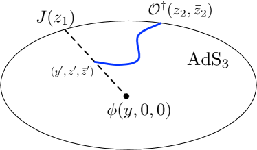
Figure 4: Witten diagram for $\langle J{\cal O}^{\dagger}\phi\rangle$

The bulk-boundary three-point function $\left\langle J\left(z_{1}\right)\mathcal{O}^{\dagger}\left(z_{2},\bar{z}_{2}\right)\phi\left(X_{1}\right)\right\rangle$ (with $X_{1}=\left(y,0,0\right)$) is computed as usual by

$$\left\langle J\mathcal{O}^{\dagger}\phi\right\rangle=\int_{\text{AdS}_{3}}\sqrt{g}d^{3}X^{\prime}\frac{1}{\left(z^{\prime}-z_{1}\right)^{2}}2iqy^{\prime 2}\left[G\partial_{\bar{z}^{\prime}}K-G\partial_{\bar{z}^{\prime}}K\right]$$ (C.30)

where where we’ve denoted $X^{\prime}=\left(y^{\prime},z^{\prime},\bar{z}^{\prime}\right)$, and also used the bulk-boundary propagator for the photons (C.29). Explicitly, the coordinate dependence of $G$ and $K$ are $G=G\left(X_{1},X^{\prime}\right)$ and $K=K\left(X^{\prime},\left(z_{2},\bar{z}_{2}\right)\right)$. Now as mentioned above, we integrate by parts to find

$$\left\langle J\mathcal{O}^{\dagger}\phi\right\rangle=-\int_{\text{AdS}_{3}}\sqrt{g}d^{3}X^{\prime}\frac{4iqy^{\prime 2}}{\left(z^{\prime}-z_{1}\right)^{2}}G\partial_{\bar{z}^{\prime}}K$$ (C.31)

Now we can do a saddle point approximation as in appendix D.4 of Anand:2017dav . The idea is as follows. We can write

$$G\left(X_{1},X^{\prime}\right)=\frac{e^{-2h\sigma_{\left(X_{1},X^{\prime}\right)}}}{1-e^{-2\sigma_{\left(X_{1},X^{\prime}\right)}}}$$ (C.32)

where $\rho\equiv e^{-2\sigma}$ and $\sigma_{\left(X_{1},X^{\prime}\right)}$ is the geodesic length between $X_{1}=\left(y,0,0\right)$ and $X^{\prime}=\left(y^{\prime},z^{\prime},\bar{z}^{\prime}\right)$, whose expression can be obtained from (C.11). Similarly, the bulk boundary propagator can be written as

$$K\left(X^{\prime},\left(z_{2},\bar{z}_{2}\right)\right)=e^{-2h\sigma_{\left(X^{\prime},\left(z_{2},\bar{z}_{2}\right)\right)}}$$ (C.33)

where $\sigma_{\left(X^{\prime},\left(z_{2},\bar{z}_{2}\right)\right)}=\log\frac{y^{\prime 2}+\left(z^{\prime}-z_{2}\right)\left(\bar{z}^{\prime}-\bar{z}_{2}\right)}{y^{\prime}}$ is the (regularized) bulk-boundary geodesic length between $X^{\prime}=\left(y^{\prime},z^{\prime},\bar{z}^{\prime}\right)$ and $\left(z_{2},\bar{z}_{2}\right)$. So the integral (C.31) after simplification can be written in the following form

$$\left\langle J\mathcal{O}^{\dagger}\phi\right\rangle=8ihq\int\frac{dz^{\prime}d\bar{z}^{\prime}dy^{\prime}}{y^{{}^{\prime}2}}e^{-2hL\left(y^{\prime},z^{\prime},\bar{z}^{\prime}\right)}\frac{e^{-\sigma_{\left(y^{\prime},z^{\prime},\bar{z}^{\prime}\right),\left(z_{2},\bar{z}_{2}\right)}}}{1-e^{-2\sigma_{\left(y,0,0\right),\left(y^{\prime},z^{\prime},\bar{z}^{\prime}\right)}}}\frac{\left(z^{\prime}-z_{2}\right)}{\left(z^{\prime}-z_{1}\right)^{2}}$$ (C.34)

where $L\left(y^{\prime},z^{\prime},\bar{z}^{\prime}\right)\equiv\sigma_{\left(X_{1},X^{\prime}\right)}+\sigma_{\left(X^{\prime},\left(z_{2},\bar{z}_{2}\right)\right)}$. Now we can take the large $h$ limit and the integration will be dominated by the line integral along the geodesic from $X_{1}=\left(y,0,0\right)$ to $\left(z_{2},\bar{z}_{2}\right)$. This geodesic parameterized by $z^{\prime}$ is given by

$$\bar{z}^{\prime}=\frac{\bar{z}}{z}z^{\prime},\quad y^{\prime 2}=\left(1-\frac{z^{\prime}}{z}\right)\left(y^{2}+z^{\prime}\bar{z}\right),$$ (C.35)

so that the saddle point approximation to equation (C.31) is

$$\langle J{\cal O}^{\dagger}\phi\rangle=8\pi iqe^{-2hL(y,0,0)}\int_{0}^{z_{2}}dz^{\prime}\frac{1}{\sqrt{|\det\partial^{2}L}|}\frac{e^{-2\sigma_{\left(X^{\prime},\left(z_{2},\bar{z}_{2}\right)\right)}}}{1-e^{-2\sigma_{\left(X_{1},X^{\prime}\right)}}}\frac{1}{y^{\prime 2}}\frac{\left(z^{\prime}-z_{2}\right)}{\left(z^{\prime}-z_{1}\right)^{2}},$$ (C.36)

where the determinant is given by

$$\det\partial^{2}L=\det\left(\begin{array}[]{cc}{\partial_{\bar{z}^{\prime}}^{2}L}&{\partial_{\bar{z}^{\prime}}\partial_{y^{\prime}}L}\\ {\partial_{y^{\prime}}\partial_{\bar{z}^{\prime}}L}&{\partial_{y^{\prime}}^{2}L}\end{array}\right)=\frac{4z_{2}^{5}\left(z^{\prime}\bar{z}_{2}+y^{2}\right)}{z^{\prime 2}\left(z^{\prime}-z_{2}\right)\left(z_{2}\bar{z}_{2}+y^{2}\right)^{4}}.$$ (C.37)

Plugging this in (C.36), we have

$$\left\langle J(z_{1})\mathcal{O}^{\dagger}(z_{2},\bar{z}_{2})\phi(y,0,0)\right\rangle=q\left\langle\phi{\cal O}^{\dagger}\right\rangle\int_{0}^{z_{2}}dz^{\prime}\frac{1}{\left(z_{1}-z^{\prime}\right)^{2}}=\frac{qz_{2}}{\left(z_{2}-z_{1}\right)z_{1}}\left\langle\phi{\cal O}^{\dagger}\right\rangle$$ (C.38)

where we’ve used the fact that $\left\langle\phi(y,0,0){\cal O}^{\dagger}(z_{2},\bar{z}_{2})\right\rangle=e^{-2hL(y,0,0)}=\left(\frac{y}{y^{2}+z_{2}\bar{z}_{2}}\right)^{2h}$ and we neglected a numerical constant in obtaining the above result. The above result is exactly the same as the result (2.22) obtained via assuming $\phi$ to be a charged bulk field defined by the bulk primary condition (2.16).

C.2.2 One-loop Correction to $\left\langle\phi^{\dagger}\phi\right\rangle$

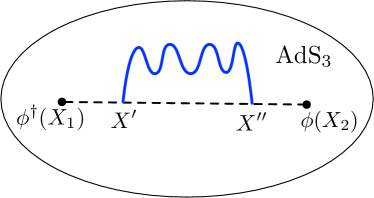
Figure 5: Witten diagram for $\langle\phi^{\dagger}\phi\rangle$

In this subsection, we are going to compute one loop correction to $\left\langle\phi^{\dagger}\phi\right\rangle$. The Witten diagram is given in figure 5, and it’s computed as follows

$$\left\langle\phi^{\dagger}\left(X_{1}\right)\phi\left(X_{2}\right)\right\rangle_{\text{1 loop}} =-16q^{2}\int\sqrt{\left|g\right|}d^{3}X^{\prime}\int\sqrt{\left|g\right|}d^{3}X^{\prime\prime}y^{\prime 2}y^{\prime\prime 2}$$ (C.39)

$$\qquad\times G\left(X_{1},X^{\prime}\right)\partial_{\bar{z}^{\prime}}G\left(X^{\prime},X^{\prime\prime}\right)H\left(X^{\prime},X^{\prime\prime}\right)\partial_{\bar{z}^{\prime\prime}}G\left(X^{\prime\prime},X_{2}\right)$$

Acting on this two-point function with the Klein-Gordon operator twice, we have

$$\left(\nabla_{1}^{2}+m^{2}\right)\left(\nabla_{2}^{2}+m^{2}\right)\left\langle\phi^{\dagger}\left(X_{1}\right)\phi\left(X_{2}\right)\right\rangle_{\text{1 loop}}=-16q^{2}H\left(X_{1},X_{2}\right)y_{1}^{2}y_{2}^{2}\partial_{\bar{z}_{1}}\partial_{\bar{z}_{2}}G\left(X_{1},X_{2}\right)$$ (C.40)

By using the photon propagator (C.24) and the bulk-bulk propagator (C.25), one can show that the RHS of the above equation is

$$-\frac{32q^{2}\rho^{h+1}\left(2h^{2}(1-\rho)^{2}+h\left(-5\rho^{2}+4\rho+1\right)+3\rho(\rho+1)\right)}{k(1-\rho)^{5}}.$$ (C.41)

Assuming $P\left(\rho\right)\equiv\left\langle\phi^{\dagger}\left(X_{1}\right)\phi\left(X_{2}\right)\right\rangle_{\text{1 loop}}$ only depends on the $\rho$, equation (C.40) becomes

$$16\left(h-1\right)^{2}h^{2}P\left(\rho\right)+\frac{64}{\rho-1}\left(-h^{2}+h+1\right)\rho^{2}P^{\prime}\left(\rho\right)$$ (C.42)

$$-\frac{32\rho^{2}\left(\left(h-1\right)h\left(\rho-1\right)-7\rho+1\right)P^{\prime\prime}\left(\rho\right)}{\rho-1}+\frac{64\rho^{3}\left(2\rho-1\right)P^{\left(3\right)}\left(\rho\right)}{\rho-1}+16\rho^{4}P^{\left(4\right)}\left(\rho\right)$$

$$= -\frac{32q^{2}\rho^{h+1}\left(2h^{2}(1-\rho)^{2}+h\left(-5\rho^{2}+4\rho+1\right)+3\rho(\rho+1)\right)}{k(1-\rho)^{5}}$$

Luckily, Mathematica is able to solve the above fourth order differential equation. Fixing the integration constants, we get

$$P\left(\rho\right)=-\frac{q^{2}}{k}\frac{\rho^{h}}{1-\rho}\left[\frac{\rho^{2}\,_{2}F_{1}(1,2h+1;2(h+1);\rho)}{2h+1}+\frac{\rho}{2h}-\log(1-\rho)\right],$$ (C.43)

which is exactly the same as the $\frac{1}{k}$ correction to the two-point function of the bulk charged proto-field computed in appendix C.1 using pure CFT technics.

Appendix D Computations of $\langle\phi\mathcal{O}T\rangle$ in Global AdS₃

In this section, we use two methods to calculate $\langle\phi\mathcal{O}T\rangle$ in global AdS₃. These two methods are essentially the same. Both of them are based on the idea of bulk-boundary OPE blocks (as we called them in Anand:2017dav and Chen:2018qzm ) or the bulk-boundary bi-local operator $\phi{\cal O}$ (D.2) (a generalization of the boundary bi-local operator as defined in Cotler:2018zff ). The first method is to expand the vacuum channel of the bulk-boundary bi-local operator in terms of the $\epsilon$ operator defined in section 6 of Cotler:2018zff , and then use the $\epsilon$ propagator, which was derived from the Alekseev-Shatashvilli theory of boundary gravitons in that paper, to compute $\left\langle\phi{\cal O}T\right\rangle$. The second method is to expand the vacuum channel of the bi-local in terms of the energy-momentum tensor $T$ and use the two-point function of $T$ to compute $\left\langle\phi{\cal O}T\right\rangle$. Both of them give the same result as (3.31) obtained using the properties of the bulk proto-field.

D.1 $\langle\phi\mathcal{O}T\rangle$ in Global AdS₃ from Alekseev-Shatashvili

The idea here very similar to that of section 5.2, where we computed the $1/c$ corrections to the bulk-boundary propagator in a heavy background. The difference is that here we are considering bulk-boundary bi-local operator $\phi{\cal O}$ in the vacuum.

As in section 3.3.2, we use $f\left(z\right)=e^{z}$ and $\bar{f}\left(\bar{z}\right)=e^{\bar{z}}$ to obtain the global AdS₃ metric (3.28). But now we are going to include perturbation as follows

$$f\left(z\right)=e^{z+i\frac{\epsilon\left(z\right)}{c}},\text{ and }\bar{f}\left(\bar{z}\right)=e^{\bar{z}-i\frac{\bar{\epsilon}\left(\bar{z}\right)}{c}}$$ (D.1)

(with $\epsilon\left(z\right)$ and $\bar{\epsilon}\left(z\right)$ promoted to operators). Specifically, the vacuum contribution to the bulk-boundary bi-local operator is given by

$$\phi\left(y_{1},z_{1},\bar{z}_{1}\right){\cal O}\left(z_{2},z_{2}\right)|_{\text{vac}}=\left(f^{\prime}\left(z_{2}\right)\bar{f}^{\prime}\left(\bar{z}_{2}\right)\right)^{h}\left(\frac{u_{1}}{u_{1}^{2}+\left(x_{1}-f\left(z_{2}\right)\right)\left(\bar{x}_{1}-f\left(\bar{z}_{2}\right)\right)}\right)^{2h}.$$ (D.2)

The $(u_{1},x_{1},\bar{x}_{1})$ here are functions of $(y_{1},z_{1},\bar{z}_{1})$ given by (3.2) with $f(z)$ and $\bar{f}(\bar{z})$ given by (D.1). One can see that the above expression becomes the boundary bi-local defined in Cotler:2018zff when we send $\phi$ to the boundary by taking $y_{1}\rightarrow 0$. Written in terms of the coordinates $\left(y,z,\bar{z}\right)$ and expanded in large $c$, the above vacuum block becomes

$$\frac{\phi\left(y_{1},z_{1},\bar{z}_{1}\right){\cal O}\left(z_{2},\bar{z}_{2}\right)|_{\text{vac}}}{\left\langle\phi\left(y_{1},z_{1},\bar{z}_{1}\right){\cal O}\left(z_{2},\bar{z}_{2}\right)\right\rangle_{\text{global AdS}_{3}}}=1+\frac{1}{c}\frac{B\epsilon_{1}+C\epsilon_{1}^{\prime}+D\epsilon_{1}^{\prime\prime}+E\epsilon_{2}+F\epsilon_{2}^{\prime}}{A}+{\cal O}\left(\frac{1}{c^{2}}\right)$$ (D.3)

where $\epsilon_{i}\equiv\epsilon\left(z_{i}\right)$ and the derivatives are with respect to $z_{i}$. The bulk-boundary propagator $\left\langle\phi\left(y_{1},z_{1},\bar{z}_{1}\right){\cal O}\left(z_{2},\bar{z}_{2}\right)\right\rangle_{\text{global AdS}_{3}}$ in global AdS₃ is given in (3.32) (up to a factor of $(\xi_{2}\bar{\xi}_{2})^{h}$ coming from the $\left(f^{\prime}\left(z_{2}\right)\bar{f}^{\prime}\left(\bar{z}_{2}\right)\right)^{h}$ in (D.2)), i.e.

$$\langle\phi\mathcal{O}\rangle_{\text{global AdS${}_{3}$}}=\left(\frac{4y_{1}\sqrt{\xi_{1}\bar{\xi}_{1}\xi_{2}\bar{\xi}_{2}}}{\left(\bar{\xi_{1}}\xi_{1}+\bar{\xi}_{2}\xi_{2}\right)\left(y_{1}^{2}+4\right)+\left(\bar{\xi}_{1}\xi_{2}+\bar{\xi}_{2}\xi_{1}\right)\left(y_{1}^{2}-4\right)}\right)^{2h},$$ (D.4)

where we’ve defined $\xi_{i}\equiv e^{z_{i}}$ and $\bar{\xi}_{i}=e^{\bar{z}_{i}}$. The denominator and the coefficients in the numerator of (D.3) are given by

$$A =i\left(\left(y_{1}^{2}-4\right)\left(\xi_{2}\bar{\xi}_{1}+\xi_{1}\bar{\xi}_{2}\right)+\left(y_{1}^{2}+4\right)\left(\xi_{1}\bar{\xi}_{1}+\xi_{2}\bar{\xi}_{2}\right)\right),$$

$$B =\left(y_{1}^{2}-4\right)\left(\xi_{1}\bar{\xi}_{2}-\xi_{2}\bar{\xi}_{1}\right)+\left(y_{1}^{2}+4\right)\left(\xi_{1}\bar{\xi}_{1}-\xi_{2}\bar{\xi}_{2}\right),$$

$$C =\left(y_{1}^{2}+4\right)\left(\xi_{2}\bar{\xi}_{1}+\xi_{1}\bar{\xi}_{2}\right)+\left(y_{1}^{2}-4\right)\left(\xi_{1}\bar{\xi}_{1}+\xi_{2}\bar{\xi}_{2}\right),$$ (D.5)

$$D =-2y_{1}^{2}\left(\xi_{1}-\xi_{2}\right)\left(\bar{\xi}_{1}+\bar{\xi}_{2}\right),$$

$$E =\left(y_{1}^{2}+4\right)\left(\xi_{2}\bar{\xi}_{2}-\xi_{1}\bar{\xi}_{1}\right)+\left(y_{1}^{2}-4\right)\left(\xi_{2}\bar{\xi}_{1}-\xi_{1}\bar{\xi}_{2}\right),$$

$$F =-\left(y_{1}^{2}-4\right)\left(\xi_{2}\bar{\xi}_{1}+\xi_{1}\bar{\xi}_{2}\right)-\left(y_{1}^{2}+4\right)\left(\xi_{1}\bar{\xi}_{1}+\xi_{2}\bar{\xi}_{2}\right).$$

We’ve only kept the holomorphic $\epsilon$ terms in (D.3), since the anti-holomorphic $\bar{\epsilon}$ will not contribute to $\left\langle\phi{\cal O}T\right\rangle$.

To compute $\left\langle\phi{\cal O}T\right\rangle$, we also need to write the energy-momentum tensor $T$ in terms of the $\epsilon$ operators. As explained in section 2 of Anand:2017dav , $T$ is simply given by the Schwarzian derivative as follows:

$$T\left(z\right)=\frac{c}{12}\left[\frac{f^{\prime\prime\prime}(z)f^{\prime}(z)-\frac{3}{2}\left(f^{\prime\prime}(z)\right)^{2}}{\left(f^{\prime}(z)\right)^{2}}\right]=-\frac{c}{24}-\frac{i}{12}\left(\epsilon^{\prime}(z)-\epsilon^{(3)}(z)\right)+{\cal O}\left(\frac{1}{c}\right).$$ (D.6)

The last piece of information we need to compute $\left\langle\phi{\cal O}T\right\rangle$ is the $\epsilon$ propagator $\left\langle\epsilon\epsilon\right\rangle$. The action obeyed by $\epsilon$ and $\bar{\epsilon}$ is the saddle point quadratic action derived from the Alekseev-Shatashvilli action. And the $\epsilon$ propagator is given in section 6 of Cotler:2016fpe ,

$$\left\langle\epsilon\left(z\right)\epsilon\left(0\right)\right\rangle=6c\left(-1+\frac{3\xi}{2}-\frac{\left(1-\xi\right)^{2}}{\xi}\ln\left(1-\xi\right)\right),\quad\xi\equiv e^{z}$$ (D.7)

Note that we have a different normalization for the $\epsilon$s.

Eventually, $\left\langle\phi\left(y_{1},z_{1},\bar{z}_{1}\right){\cal O}\left(z_{2},\bar{z}_{2}\right)T\left(z\right)\right\rangle$ is given by

$$\frac{\left\langle\phi{\cal O}T\right\rangle}{\left\langle\phi{\cal O}\right\rangle_{\text{global AdS${}_{3}$}}}=\frac{h\left(\xi_{1}-\xi_{2}\right)^{2}\xi^{2}}{\left(\xi-\xi_{1}\right)^{3}\left(\xi-\xi_{2}\right)^{2}}\left[\xi-\xi_{1}+\frac{4y_{1}^{2}\xi_{1}\left(\xi-\xi_{2}\right)\left(\bar{\xi}_{1}+\bar{\xi}_{2}\right)}{\left(\bar{\xi}_{1}\xi_{1}+\bar{\xi}_{2}\xi_{2}\right)\left(y_{1}^{2}+4\right)+\left(\bar{\xi}_{1}\xi_{2}+\bar{\xi}_{2}\xi_{1}\right)\left(y_{1}^{2}-4\right)}\right]-\frac{c}{24}$$ (D.8)

which agrees with (3.31) up to a trivial transformation for ${\cal O}$ and $T$ from the complex plane $\left(\xi,\bar{\xi}\right)$ to the cylinder $\left(z,\bar{z}\right)$.

D.2 $\langle\phi\mathcal{O}T\rangle$ in Global AdS₃ from $\langle TT\rangle$

We can also compute $\left\langle\phi{\cal O}T\right\rangle$ in global AdS₃ without using the $\epsilon$ propagator as we did in last subsection. Instead, we’ll use the two-point function of the energy-momentum tensor $T$. This was the method that we used in Anand:2017dav to compute $\left\langle\phi{\cal O}T\right\rangle$ (equation (3.26)) in Poincare AdS₃, and also in appendix B of Chen:2018qzm to compute the $1/c$ corrections to the vacuum block of all-light bulk-boundary correlator $\left\langle{\cal O}_{2}{\cal O}_{2}\phi_{1}{\cal O}_{1}\right\rangle$ (with $\phi_{1}$ the proto-field of section 3.1) up to order $1/c^{2}$.

The idea is actually very similar to that of last section. Instead of denoting the perturbation via $\epsilon$, we expand $f\left(z\right)$ in the large $c$ limit as

$$f(z)=e^{z}+\frac{1}{c}f_{1}(z)+\dots,$$ (D.9)

and similarly for $\bar{f}\left(\bar{z}\right)$. Then similar to last subsection, the energy-momentum tensor $T\left(z\right)$ is given by

$$T(z)=\frac{c}{12}\left[\frac{f^{\prime\prime\prime}(z)f^{\prime}(z)-\frac{3}{2}\left(f^{\prime\prime}(z)\right)^{2}}{\left(f^{\prime}(z)\right)^{2}}\right] =-\frac{c}{24}+\frac{1}{12}e^{-z}\left(2f_{1}^{\prime}-3f_{1}^{\prime\prime}+f_{1}^{\left(3\right)}\right)+O\left(\frac{1}{c}\right).$$ (D.10)

The energy-momentum tensor $T\left(\xi\right)$ on the complex plane with coordinates $\left(\xi=e^{z},\bar{\xi}=e^{\bar{z}}\right)$ is related to $T\left(z\right)$ as usual by

$$T\left(z\right)=-\frac{c}{24}+\xi^{2}T\left(\xi\right),$$ (D.11)

so from (D.10), we have

$$T\left(e^{z}\right)=\frac{1}{12}e^{-3z}\left(2f_{1}^{\prime}-3f_{1}^{\prime\prime}+f_{1}^{\left(3\right)}\right)$$ (D.12)

We can now solve for $f_{1}\left(z\right)$ in terms of $T\left(e^{z}\right)$, and the solution is given by

$$f_{1}(z)=12\int_{0}^{z}\left(\int_{0}^{z^{\prime}}e^{z^{\prime}+z^{\prime\prime}}(e^{z^{\prime}}-e^{z^{\prime\prime}})T\left(e^{z^{\prime\prime}}\right)\,\,dz^{\prime\prime}\right)dz^{\prime}.$$ (D.13)

The bulk-boundary OPE block or the bulk boundary bi-local operator (D.2) can then be expanded in large $c$,

$$\frac{\phi\left(y,0,0\right){\cal O}\left(z_{2},\bar{z}_{2}\right)|_{\text{vac}}}{\left\langle\phi\left(y,0,0\right){\cal O}\left(z_{2},\bar{z}_{2}\right)\right\rangle_{\text{global AdS}_{3}}}=1+\frac{1}{c}\left(\frac{hf_{1}^{\prime}\left(z_{2}\right)}{\xi_{2}}-\frac{2h\left(\left(y^{2}+4\right)\bar{\xi}_{2}+y^{2}-4\right)f_{1}\left(z_{2}\right)}{\left(y^{2}+4\right)\left(1+\bar{\xi}_{2}\xi_{2}\right)+\left(y^{2}-4\right)\left(\xi_{2}+\bar{\xi}_{2}\right)}\right)+O\left(\frac{1}{c^{2}}\right)$$ (D.14)

Using $\left\langle T\left(e^{z}\right)T\left(e^{z_{2}}\right)\right\rangle=\frac{c}{\left(e^{z}-e^{z_{2}}\right)^{4}}$ on the complex plane, we find

$$\left\langle f_{1}\left(z_{2}\right)T\left(e^{z}\right)\right\rangle =\frac{c\left(\xi_{2}-1\right)^{3}}{(\xi-1)^{3}\left(\xi-\xi_{2}\right)}$$ (D.15)

$$\left\langle f_{1}^{\prime}\left(z_{2}\right)T\left(e^{z}\right)\right\rangle =-\frac{c\left(\xi_{2}-1\right)^{2}\xi_{2}\left(1-3\xi+2\xi_{2}\right)}{(\xi-1)^{3}\left(\xi-\xi_{2}\right)^{2}}$$

and $\left\langle\phi\left(y,0,0\right){\cal O}\left(z_{2},\bar{z}_{2}\right)T\left(z\right)\right\rangle$ (after transforming $T$ to the cylinder) is given by

$$\frac{\left\langle\phi{\cal O}T\right\rangle}{\left\langle\phi{\cal O}\right\rangle_{\text{global AdS${}_{3}$}}}=\frac{h\left(1-\xi_{2}\right)^{2}\xi^{2}}{\left(\xi-1\right)^{3}\left(\xi-\xi_{2}\right)^{2}}\left[\xi-1+\frac{4y_{1}^{2}\left(\xi-\xi_{2}\right)\left(1+\bar{\xi}_{2}\right)}{\left(1+\bar{\xi}_{2}\xi_{2}\right)\left(y^{2}+4\right)+\left(\xi_{2}+\bar{\xi}_{2}\right)\left(y^{2}-4\right)}\right]-\frac{c}{24}$$ (D.16)

which is exactly the result obtained in last subsection (D.8) with $y_{1}=y,z_{1}=\bar{z}_{1}=0$.