Two-dimensional melting via sine-Gordon duality

Abstract

Motivated by the recently developed duality [Pretko and Radzihovsky, Phys. Rev. Lett. 120, 195301 (2018)] between the elasticity of a crystal and a symmetric tensor gauge theory, we explore its classical analog, which is a dual theory of the dislocation-mediated melting of a two-dimensional crystal, formulated in terms of a higher derivative vector sine-Gordon model. It provides a transparent description of the continuous two-stage melting in terms of the renormalization-group relevance of two cosine operators that control the sequential unbinding of dislocations and disclinations, respectively corresponding to the crystal-to-hexatic and hexatic-to-isotropic fluid transitions. This renormalization-group analysis reproduces the seminal results of the Coulomb gas description, such as the flows of the elastic couplings and of the dislocation and disclination fugacities, as well as the temperature dependence of the associated correlation lengths.

I Introduction

I.1 Background and motivation

The theory of continuous two-dimensional (2D) melting, developed by Kosterlitz and ThoulessKosterlitz 72 , Halperin and NelsonNelson 79 , and YoungYoung 79 (KTHNY), building on the work of LandauLandau 37 , PeierlsPeierls 35 and BerezinskiiBerezinskii 71 ; Berezinskii 72 , has become one of the pillars of theoretical physics. Mathematically related to simpler normal-to-superfluid and planar paramagnet-to-ferromagnet transitions in films, described by a 2D XY model, it is a striking example of the increased importance of thermal fluctuations in low-dimensional systemsHalperin 79 ; Nelson 83 . In contrast to their bulk three-dimensional analogs, where, typically, fluctuations only lead to quantitative modifications of mean-field predictions (e.g., values of critical exponents), here the effects are qualitative and drastic. Located exactly at the lower-critical dimension, a local-order-parameter distinction between the high- and low-temperature phases that is erased by fluctuations, two-dimensional melting can proceed via a subtle, two-stage, continuous transition, driven by the unbinding of topological dislocations and disclinations defects. This mechanism, made possible by strong thermal fluctuations, thus provides an alternative route to direct first-order melting, argued by Landau’s mean-field analysisLandau 37 to be the exclusive scenario.

As such, the continuous two-dimensional melting (and related disordering of a 2D XY model) is the earliest example of a thermodynamically sharp, topological phase transition between two locally disordered phases, which thus does not admit Landau’s local order-parameter description. It is controlled by a fixed line, which lends itself to an asymptotically exact analysisKosterlitz 72 ; Nelson 79 ; Young 79 .

Although evidence for defects-driven phase transitions has appeared in a number of experiments on liquid crystalsHuang 93 and Langmuir-Blodgett filmsKnobler 07 , finding simple model systems that exhibit these phenomena in experiments or simulations has proven to be more challenging. Most studied systems appear to exhibit discontinuous first-order melting that converts a crystal directly into a liquid. However, it appears that two-stage continuous melting has been experimentally observed by MurrayMurray 88 and ZahnZahn 99 in beautiful melting experiments on two-dimensional colloids confined between smooth glass plates and superparamagnetic colloidal systems, respectively. In these experiments, an orientationally quasi-long-range ordered but translationally disordered hexatic phaseNelson 79 was indeed observed. As was first emphasized by Halperin and NelsonNelson 79 , the hexatic liquid, intermediate but thermodynamically distinct from the 2D crystal and the isotropic liquid, is an important signature of the defect-driven two-stage melting. In these two-dimensional colloids, particle positions and the associated topological defects can be directly imaged via digital video-microscopy, allowing precise quantitative tests of the theory.

I.2 Duality of the two-stage melting transition

The disordering of the simpler 2D XY model (describing, e.g., a superfluid-normal transition in a film) is well known to admit two complementary descriptions, the 2D Coulomb gas of vorticesCoulombGas and its dual sine-Gordon field theorysineGordon ; sineGordonKT ; Nelson 79 ; Halperin 79 ; ChaikinLubensky ; RadzihovskyLubensky . As with other dualities – a subject with long history and of much current interestSenthil 18 – the sine-Gordon duality has been extensively utilized in a variety of physical contexts. Given that elasticity of a crystal can be thought of as a space-spin coupled vector generalization of an XY model (with vector phonon Goldstone modes $u_{x},u_{y}$ replacing the scalar phase angle), it is of interest also to develop an analogous dual sine-Gordon formulation and to use it to study the 2D continuous melting transition.

Indeed, recently, such a complementary description has emerged as a classical limit of the elasticity-to-tensor gauge theory dualityPretkoRL 18/05 ; PretkoRL 18/12 , derived in the context of a new class of topologically-ordered fracton matterNandkishore 18 . As we will detail in the body of the paper the corresponding dual Hamiltonian is given by

$$\begin{split}\tilde{H}&=\int d^{2}r\left[\frac{1}{2}\tilde{C}^{-1}_{ij,kl}\partial_{i}\partial_{j}\phi\partial_{k}\partial_{l}\phi\right.\\ &\left.-g_{b}\sum_{n=1}^{p}\cos({\bf b}_{n}\cdot\hat{{\bf z}}\times{\bm{\nabla}}\phi)-g_{s}\cos(s_{p}\phi)\right].\end{split}$$ (1)

Its key features, which characterize the continuous two-stage melting are the higher-order “Laplacian elasticity”, encoded via elastic constants $\tilde{C}^{-1}_{ij,kl}$, and two sine-Gordon types of operators with couplings $g_{b},g_{s}$, respectively, capturing the importance (fugacities) of dislocation (elementary vector charges ${\bf b}_{n}$) and disclination (elementary scalar charge $s_{p}$) defects.

To flesh out the essence of this dual description, neglecting inessential details, the above Hamiltonian is schematically described by

$$\tilde{H}\sim\int_{\bf r}\left[{\frac{1}{2}}\tilde{C}(\partial^{2}\phi)^{2}-g_{b}\cos(\partial\phi)-g_{s}\cos(\phi)\right],$$ (2)

where $\int_{\bf r}\equiv\int d^{2}r$. Because of the second-order Laplacian elasticity, standard analysis around the Gaussian fixed line $g_{b}=g_{s}=0$ shows that the mean-squared fluctuations of Airy-stress potential $\phi$ diverge quadratically with system size. This leads to an exponentially (as opposed to power-law in a conventional sine-Gordon model) vanishing Debye-Waller factor, and in turn to a strongly irrelevant disclination cosine, $g_{s}$, that can therefore be neglected, whenever $g_{b}$ is small, i.e., near the Gaussian fixed line.

The schematic Hamiltonian then reduces to

$$\tilde{H}_{\text{cr}}\sim\int_{\bf r}\left[{\frac{1}{2}}\tilde{C}(\partial\chi)^{2}-g_{b}\cos(\chi)\right],$$ (3)

with $\chi=\partial\phi$. It thus obeys the standard sine-Gordon phenomenology, exhibiting a KT-like “roughenning” transition in $\chi$ with the relevance of $g_{b}$, controlled by the stiffness $\tilde{C}$.sineGordon ; sineGordonKT ; Nelson 79 ; Halperin 79 ; ChaikinLubensky At small $\tilde{C}<\tilde{C}_{c}$, $g_{b}$ is irrelevant, describing the gapless crystal phase, with confined dislocations and disclinations. The melting of the crystal is then captured by the relevance of $g_{b}$ for $\tilde{C}>\tilde{C}_{c}$, corresponding to a transition into a plasma of unbound dislocatons characteristic of a hexatic fluid. Since in this phase $g_{b}$ is relevant, at sufficiently long scales the dislocation cosine in Eq. $(2)$ reduces to a harmonic potential for $\chi$, $-g_{b}\cos(\partial\phi)\sim{\frac{1}{2}}g_{b}(\partial\phi)^{2}$. The effective Hamiltonian is then given by

$$\tilde{H}_{\text{hex}}\sim\int_{\bf r}\left[{\frac{1}{2}}g_{b}(\partial\phi)^{2}-g_{s}\cos(\phi)\right],$$ (4)

where we have neglected the $\tilde{C}$ “curvature” elasticity relative to the gradient one encoded in $g_{b}$, and restored the disclination cosine operator $g_{s}\cos(\phi)$. The resulting conventional sine-Gordon model in $\phi$ can then exhibit the second KT-like “roughenning” transition, capturing the hexatic-to-isotropic fluid transition, asssociated with the unbinding of disclinations. The corresponding RG flow of the dual vector sine-Gordon model is schematically illustrated in Fig. 1. We leave the detailed analysis of this two-stage melting transition to the main body of the paper and the Appendix.

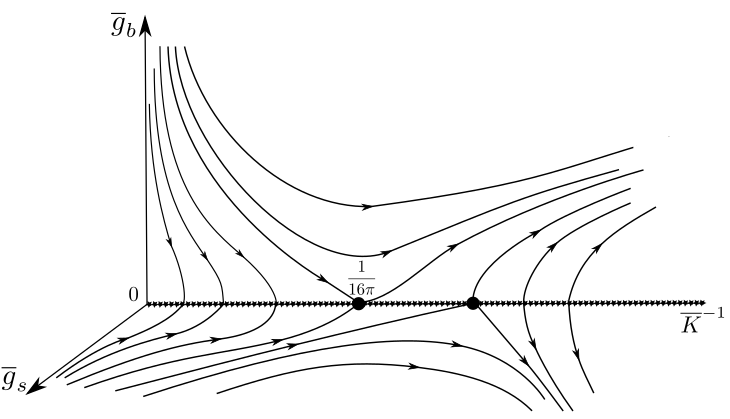
Figure 1: A schematic illustration of RG flows in the dual vector sine-Gordon model. It describes the two-stage continuous 2D melting, crystal-to-hexatic and hexatic-to-isotropic liquid transitions, associated with the consequent relevance of dislocations ($g_{b}$) and disclinations ($g_{s}$) fugacities, as a function of the elastic modulus ${\bar{K}}^{-1}=\frac{2\mu+\lambda}{4a^{2}\mu(\mu+\lambda)}$, expressed in terms of the Lamé elastic constants, $\mu,\lambda$ (defined in the main text) and the lattice constant $a$.

I.3 Outline

The rest of this paper is organized as follows. In Sec. II, after briefly reviewing the elasticity theory of two-dimensional crystal and its topological defects, we give two detailed complementary derivations of the duality transformation to the vector sine-Gordon model. Utilizing the latter we straightforwardly reproduce known results for the crystal-hexatic phase transition in Sec. III, by focusing on the dislocation fugacity cosine operator and neglecting the irrelevant disclinations. Inside the hexatic phase, we derive a scalar sine-Gordon model for the Airy stress potential, that captures the subsequent hexatic-isotropic liquid transition. We conclude in Sec. IV with a summary of our results and a discussion of potential applications of this dual approach.

II Duality of 2D melting

II.1 Two-dimensional elasticity

At low temperatures, the deformations of a crystal do not vary substantially over the atom size, allowing it to be described with a continuum field theory of its phonon Goldstone modes, $u({\bf r})$, with a short-distance cutoff set by the lattice spacing $a$. The underlying translational symmetry (spontaneously broken by the crystal), requires that the elastic energy is an analytic expansion in the strain field $\partial_{i}u_{j}$. Due to the underlying rotational symmetry in the target space (i.e., no substrates and/or external fields), the elastic Hamiltonian is further constrained (in harmonic order) to be independent of the antisymmetric part of $\partial_{i}u_{j}$, i.e., of the local bond angle $\theta({\bf r})=\frac{1}{2}\epsilon_{ij}\partial_{i}u_{j}=\frac{1}{2}\hat{\bf z}\cdot{\bm{\nabla}}\times{\bf u}$. The elastic Hamiltonian density to harmonic order is thus given by

$$\mathcal{H}=\frac{1}{2}C_{ij,kl}u_{ij}u_{kl},$$ (5)

where $u_{ij}=\frac{1}{2}(\partial_{i}{\bf r}\cdot\partial_{j}{\bf r}-\delta_{ij})$ is the symmetric nonlinear strain tensor (fully rotationally invariant in the target space), which in the harmonic approximation takes the linear symmetrized form

$$u_{ij}\approx\frac{1}{2}(\partial_{i}u_{j}+\partial_{j}u_{i}).$$ (6)

$C_{ij,kl}$ is the elastic constant tensor, whose number of independent components is restricted by the symmetry of the crystal. For simplicity, we focus on the isotropic hexagonal lattice, where $C_{ij,kl}$ takes the form

$$C_{ij,kl}=\lambda\delta_{ij}\delta_{kl}+2\mu\delta_{ik}\delta_{jl}$$ (7)

and characterized by two independent elastic constants, namely the Lamé coefficients, $\lambda$ and $\mu$. As we discuss in Appendix B, an external stress $\sigma^{e}_{ij}({\bf r})$ is included through an additional term $-\sigma^{e}_{ij}u_{ij}$, here focusing on the case of a vanishing external stress.

II.2 Topological defects

In addition to the single-valued elastic phonon fields, the crystal also exhibits topological defects – disclinations and dislocations, captured by including a nonsingle-valued part of the phonon distortion field.

Disclinations are topological defects associated with orientational order. A disclination at a point ${\bf r}_{0}$, illustrated in Fig. 2(a), is defined by a nonzero closed line-integral of the gradient of the bond angle around ${\bf r}_{0}$:

$$\oint_{{\bf r}_{0}}d\theta=\frac{2\pi}{p}s$$ (8)

or equivalently in a differential form:

$$\hat{\bf z}\cdot{\bm{\nabla}}\times{\bm{\nabla}}\theta=\frac{2\pi}{p}s\delta^{2}({\bf r}-{\bf r}_{0})\equiv\frac{2\pi}{p}s({\bf r}),$$ (9)

measuring the deficit/surplus bond angle, $(2\pi/p)s$, with $s$ the integer disclination charge in a $C_{p}$ symmetric crystal. In the case of a hexagonal lattice, $p=6$. In the above equation, $s({\bf r})$ is the disclination charge density.

Dislocations are vector topological defects associated with translational order. A dislocation at ${\bf r}_{0}$ with a Burgers vector-charge ${\bf b}_{n}$ (that is an elementary lattice vector), as illustrated in Fig. 2(b), is defined by a closed line-integral

$$\oint_{{\bf r}_{0}}d{\bf u}={\bf b}_{n},$$ (10)

or equivalently in the differential form,

$$\hat{\bf z}\cdot{\bm{\nabla}}\times{\bm{\nabla}}u_{i}=b_{i,n}\delta^{2}({\bf r}-{\bf r}_{0})\equiv b_{i}({\bf r}),$$ (11)

where ${\bf b}({\bf r})$ is the Burgers charge density. As illustrated in Fig. 2(b), a dislocation is a disclination dipole, and it is therefore energetically less costly than a bare disclination charge.

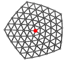
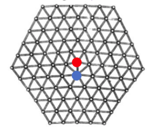
Figure 2: Topological defects in a 2D hexagonal lattice. (a) A disclination. (b) A dislocation; a dipole of two, opposite charge disclinations. (Figure adapted from Ref. [20].)

II.3 Vector Coulomb gas formulation

In the presence of topological defects, the distortion field ${\bf u}({\bf r})$ is not single-valued. Along with the associated strain tensor, the distortion field can be decomposed into the single-valued elastic phonon and the singular parts,

$$u_{i} = \tilde{u}_{i}+u_{i}^{s},$$ (12)

$$u_{ij} = \tilde{u}_{ij}+u_{ij}^{s}.$$ (13)

To include these topological and phonon degrees of freedom we focus on the partition function (taking $k_{B}T=1$, i.e., measuring coupling constants in units of thermal energy),

$$\begin{split}Z&=\int[d{\bf u}]e^{-\int_{\bf r}\mathcal{H}[{\bf u}]}\\ &=\int[d{\bf\tilde{u}}][d{\bf u}^{s}]\int[d\sigma_{ij}({\bf r})]e^{-\int_{\bf r}\mathcal{H}[{\bf u},\sigma_{ij}]},\end{split}$$ (14)

where the trace over ${\bf u}({\bf r})$ implicitly includes both phonons and topological defects by allowing nonsingle-valued distortions. In the second form, above, we decoupled the elastic energy by introducing a Hubbard-Stratonovich tensor field – the symmetric stress tensor $\sigma_{ij}({\bf r})$ChaikinLubensky , with the resulting Hamiltonian density given by

$$\begin{split}\mathcal{H}[{\bf u},\sigma_{ij}]&=\frac{1}{2}C^{-1}_{ij,kl}\sigma_{ij}\sigma_{kl}+i\sigma_{ij}u_{ij}\\ &=\frac{1}{2}C^{-1}_{ij,kl}\sigma_{ij}\sigma_{kl}+i\sigma_{ij}\left(\partial_{i}\tilde{u}_{j}+u_{ij}^{s}\right).\end{split}$$ (15)

Above, for a 2D hexagonal lattice,

$$C^{-1}_{ij,kl}=-\frac{\lambda}{4\mu(\mu+\lambda)}\delta_{ij}\delta_{kl}+\frac{1}{2\mu}\delta_{ik}\delta_{jl}$$ (16)

Tracing over the single-valued phonons $\tilde{\bf u}$, enforces the divergenless stress constraint [via $\delta$-function identity $\frac{1}{2\pi}\int_{-\infty}^{\infty}due^{iuf}=\delta(f)$]

$$\partial_{i}\sigma_{ij}=0,$$ (17)

solved with a scalar Airy stress potential, $\phi({\bf r})$,

$$\sigma_{ij}=\epsilon_{ik}\epsilon_{jl}\partial_{k}\partial_{l}\phi.$$ (18)

Expressing the Hamiltonian density in terms of $\phi({\bf r})$, and integrating by parts in the second linear term, we utilize the defects conditions, Eq. (9) and (11),

$$\epsilon_{ik}\epsilon_{jl}\partial_{l}\partial_{k}u_{ij}^{s} = \epsilon_{ik}\epsilon_{jl}\partial_{l}\partial_{k}(\partial_{i}u_{j}^{s}-\epsilon_{ij}\theta^{s}),$$ (19a)

$$= \epsilon_{ki}\partial_{k}b_{i}({\bf r})+\epsilon_{ki}\partial_{k}\partial_{i}\theta({\bf r}),$$ (19b)

$$= {\hat{\bf z}}\cdot{\bm{\nabla}}\times{\bf b}+\frac{2\pi}{6}s({\bf r}),$$ (19c)

to obtain

$$\mathcal{H}[\phi] = \frac{1}{2}\tilde{C}_{ij,kl}^{-1}\partial_{i}\partial_{j}\phi\partial_{k}\partial_{l}\phi+i\phi\left(\frac{2\pi}{6}s+{\hat{\bf z}}\cdot{\bm{\nabla}}\times{\bf b}\right).$$

Above $\tilde{C}^{-1}_{ij,kl}=\epsilon_{ia}\epsilon_{jb}\epsilon_{kc}\epsilon_{ld}C^{-1}_{ab,cd}$.

Focussing on dislocations and neglecting the high energy disclination defects, we can straightforwardly integrate out $\phi({\bf r})$ in the partition function, obtaining a dislocations vector Coulomb gas Hamiltonian

$$H_{\bf b}=\frac{1}{2}\int\frac{d^{2}q}{(2\pi)^{2}}b_{i}({\bf q})\tilde{K}_{ij}({\bf q})b_{j}(-{\bf q}),$$ (21)

where the tensor Coulomb interaction in Fourier and coordinate spaces is given by

$$\tilde{K}_{ij}({\bf q}) = \frac{K}{q^{2}}\left(\delta_{ij}-\frac{q_{i}q_{j}}{q^{2}}\right),$$ (22)

$$K_{ij}({\bf r}) = -\frac{K}{4\pi}\left(\delta_{ij}\ln(r/a)-\frac{r_{i}r_{j}}{r^{2}}\right),$$ (23)

with $K=\frac{4\mu(\mu+\lambda)}{2\mu+\lambda}$.

Thus, dislocations vector Coulomb gas Hamiltonian in real space reduces to,

$$\begin{split}H_{\bf b}&=-\frac{K}{8\pi}\int_{{\bf r}_{1},{\bf r}_{2}}\left[{\bf b}({\bf r}_{1})\cdot{\bf b}({\bf r}_{2})\ln\frac{|{\bf r}_{1}-{\bf r}_{2}|}{a}\right.\\ &\left.-\frac{{\bf b}({\bf r}_{1})\cdot({\bf r}_{1}-{\bf r}_{2})({\bf r}_{1}-{\bf r}_{2})\cdot{\bf b}({\bf r}_{2})}{|{\bf r}_{1}-{\bf r}_{2}|^{2}}\right],\end{split}$$ (24)

which, in the discrete form and supplemented with core energies (see below) is exactly the vector Coulomb gas model used by Nelson and HalperinNelson 79 and by YoungYoung 79 , as the theory of 2D continuous two-stage melting.

II.4 Dual vector sine-Gordon model

Motivated by the sine-Gordon description of the XY model, we dualize elasticity by transforming the above vector Coulomb gas into a vector sine-Gordon model and re-examine the two-stage continuous 2D melting transition from this complementary approach.

Dislocation and disclination densities on a hexagonal lattice are given as a sum of their discrete charges

$${\bf b}({\bf r}) = \sum_{{\bf r}_{n}}{\bf b}_{{\bf r}_{n}}\delta^{2}({\bf r}-{\bf r}_{n}),$$ (25)

$$s({\bf r}) = \sum_{{\bf r}_{n}}s_{{\bf r}_{n}}\delta^{2}({\bf r}-{\bf r}_{n}),$$ (26)

where ${\bf r}_{n}=a(n_{1}\hat{\bf e}_{1}+n_{2}\hat{\bf e}_{2})$, ($n_{1},n_{2}\in\mathbb{Z}$) are triangular lattice vectors spanned by unit vectors $\hat{\bf e}_{1}=\hat{\bf x}$ and $\hat{\bf e}_{2}=\frac{1}{2}\hat{\bf x}+\frac{\sqrt{3}}{2}\hat{\bf y}$, and ${\bf b}_{{\bf r}_{n}}=a(n_{1}\hat{\bf e}_{1}+n_{2}\hat{\bf e}_{2})$, and $s_{{\bf r}_{n}}\in\mathbb{Z}$ are dislocation and disclination charges, respectively.

In terms of these discrete topological defect charges, the Hamiltonian is given by

$$H= \frac{1}{2}\int_{{\bf r}}\,\tilde{C}^{-1}_{ij,kl}\partial_{i}\partial_{j}\phi\partial_{k}\partial_{l}\phi+\sum_{{\bf r}_{n}}\left[\tilde{E}_{b}{\bf b}^{2}_{{\bf r}_{n}}+E_{s}s^{2}_{{\bf r}_{n}}\right]$$ (27)

$$+\sum_{{\bf r}_{n}}\left[i\frac{2\pi}{6}\phi({\bf r}_{n})s_{{\bf r}_{n}}-i\hat{\bf z}\times{\bm{\nabla}}\phi({\bf r}_{n})\cdot{\bf b}_{{\bf r}_{n}}\right],$$

where we have added dislocation and disclination core energies $E_{b}=a^{2}\tilde{E}_{b}$ and $E_{s}$ to account for the defects’ energetics at the scales of the lattice constant, not accounted for by the elasticity theoryNelson 79 . The partition function involves an integration over potential $\phi({\bf r}_{n})$ and summation over the dislocation and disclination charges. Following a standard analysisKosterlitz 72 ; Nelson 79 ; CoulombGas ; sineGordon ; ChaikinLubensky ,

$$\begin{split}Z=&\int[d\phi]\sum_{\{s_{{\bf r}_{n}}\}}\sum_{\{{\bf b}_{{\bf r}_{n}}\}}\prod_{{\bf r}_{n}}e^{-H[\phi,{{\bf b}_{{\bf r}_{n}}},{s_{{\bf r}_{n}}}]},\\ =&\int[d\phi]e^{-{\frac{1}{2}}\int_{{\bf r}}\tilde{C}_{ij,kl}^{-1}\partial_{i}\partial_{j}\phi\partial_{k}\partial_{l}\phi}\sum_{\{s_{{\bf r}_{n}}\}}\sum_{\{{\bf b}_{{\bf r}_{n}}\}}\prod_{{\bf r}_{n}}\left[e^{-i\frac{2\pi}{6}\phi({\bf r}_{n})s_{{\bf r}_{n}}-E_{s}s_{{\bf r}_{n}}^{2}}e^{i{\hat{\bf z}}\times{\bm{\nabla}}\phi({\bf r}_{n})\cdot{\bf b}_{{\bf r}_{n}}-\tilde{E}_{b}b_{{\bf r}_{n}}^{2}}\right],\\ =&\int[d\phi]e^{-{\frac{1}{2}}\int_{{\bf r}}\tilde{C}_{ij,kl}^{-1}\partial_{i}\partial_{j}\phi\partial_{k}\partial_{l}\phi}\left[1+e^{-2E_{s}}\int\frac{d^{2}r_{1}}{a^{2}}\frac{d^{2}r_{2}}{a^{2}}e^{-i\frac{2\pi}{6}\phi({\bf r}_{1})}e^{i\frac{2\pi}{6}\phi({\bf r}_{2})}+\ldots\right]\\ &\left[1+e^{-2E_{b}}\sum_{n=1}^{3}\int\frac{d^{2}r_{1}}{a^{2}}\frac{d^{2}r_{2}}{a^{2}}e^{-i{\hat{\bf z}}\times{\bm{\nabla}}\phi({\bf r}_{1})\cdot{\bf b}_{n}}e^{i{\hat{\bf z}}\times{\bm{\nabla}}\phi({\bf r}_{2})\cdot{\bf b}_{n}}+\ldots\right],\\ =&\int[d\phi]e^{-{\frac{1}{2}}\int_{{\bf r}}\tilde{C}_{ij,kl}^{-1}\partial_{i}\partial_{j}\phi\partial_{k}\partial_{l}\phi}\cdot\left[1+e^{-E_{s}}\int\frac{d^{2}r_{1}}{a^{2}}\left(e^{i\frac{2\pi}{6}\phi({\bf r}_{1})}+e^{-i\frac{2\pi}{6}\phi({\bf r}_{1})}\right)\right.\\ &\left.+\frac{1}{2!}e^{-2E_{s}}\int\frac{d^{2}r_{1}}{a^{2}}\frac{d^{2}r_{2}}{a^{2}}\left(e^{i\frac{2\pi}{6}\phi({\bf r}_{1})}+e^{-i\frac{2\pi}{6}\phi({\bf r}_{1})}\right)\left(e^{i\frac{2\pi}{6}\phi({\bf r}_{2})}+e^{-i\frac{2\pi}{6}\phi({\bf r}_{2})}\right)+\ldots\right]\\ &\prod_{n=1,2,3}\left[1+e^{-E_{b}}\int\frac{d^{2}{r}_{1}}{a^{2}}\left(e^{i{\hat{\bf z}}\times{\bm{\nabla}}\phi({\bf r}_{1})\cdot{\bf b}_{n}}+e^{-i{\hat{\bf z}}\times{\bm{\nabla}}\phi({\bf r}_{1})\cdot{\bf b}_{n}}\right)\right.\\ &\left.+\frac{1}{2!}e^{-2E_{b}}\int\frac{d^{2}r_{1}}{a^{2}}\frac{d^{2}r_{2}}{a^{2}}\left(e^{i{\hat{\bf z}}\times{\bm{\nabla}}\phi({\bf r}_{1})\cdot{\bf b}_{n}}+e^{-i{\hat{\bf z}}\times{\bm{\nabla}}\phi({\bf r}_{1})\cdot{\bf b}_{n}}\right)\left(e^{i{\hat{\bf z}}\times{\bm{\nabla}}\phi({\bf r}_{2})\cdot{\bf b}_{n}}+e^{-i{\hat{\bf z}}\times{\bm{\nabla}}\phi({\bf r}_{2})\cdot{\bf b}_{n}}\right)+\ldots\right],\\ \equiv&\int[d\phi]e^{-\tilde{H}},\end{split}$$ (28)

where non-neutral charge configurations vanish automatically after integration over $\phi({\bf r})$. In the last step, above, we have summed over only the positive/negative single charges of dislocation and disclination, and we obtain the dual vector sine-Gordon Hamiltonian,

$$\tilde{H}= \int_{{\bf r}}\left[\frac{1}{2}\tilde{C}^{-1}_{ij,kl}\partial_{i}\partial_{j}\phi\partial_{k}\partial_{l}\phi\right.$$ (29)

$$\left.-g_{b}\sum_{n=1}^{3}\cos({\bf b}_{n}\cdot\hat{\bf z}\times{\bm{\nabla}}\phi)-g_{s}\cos\left(\frac{2\pi}{6}\phi\right)\right].$$

Above, the couplings $g_{b}=\frac{2}{a^{2}}e^{-E_{b}},g_{s}=\frac{2}{a^{2}}e^{-E_{s}}$ are proportional to dislocation and disclination fugacities, and the three elementary dislocation Burgers vectors are given by ${\bf b}_{1}=a\hat{\bf x},{\bf b}_{2}=-\frac{a}{2}\hat{\bf x}+\frac{a\sqrt{3}}{2}\hat{\bf y},{\bf b}_{3}=-{\bf b}_{1}-{\bf b}_{2}=-\frac{a}{2}\hat{\bf x}-\frac{a\sqrt{3}}{2}\hat{\bf y}$.

II.5 Vector sine-Gordon duality redux

The above derivation of the dual vector sine-Gordon model departed from the conventional phonon-only elastic model of a 2D crystal, Eq. (5). As discussed in Sec. II.2 target space rotational invariance of the crystal is incorporated by building the theory based on the symmetric tensor part $u_{ij}$, Eq. (6) of the full strain tensor, $\partial_{i}u_{j}$, i.e., forbidding an explicit dependence on the local bond angle $\theta={\frac{1}{2}}\epsilon_{ij}\partial_{i}u_{j}$, which corresponds to an angle of rotation of the crystal.

Alternatively, the rotational invariance of a crystal can be formulated as a gauge-like (minimal) coupling between the full strain tensor $\partial_{i}u_{j}$ and the bond angle $\theta({\bf r})$, encoded in the Hamiltonian density

$$\begin{split}\mathcal{H}&=\frac{1}{2}C_{ij,kl}(\partial_{i}u_{j}-\theta\epsilon_{ij})(\partial_{k}u_{l}-\theta\epsilon_{kl})+\frac{1}{2}K(\partial_{i}\theta)^{2}.\end{split}$$ (30)

It can be straightforwardly verified that an integration over the bond-angle field $\theta$ Higgs’es outRadzihovskyLubensky ; ChaikinLubensky the antisymmetric component of the strain tensor, at long wavelengths recovering the conventional elastic Hamiltonian in (5).

We now decouple the strain and bond elastic terms by introducing two Hubbard-Stratanovich fields – the stress field $\sigma_{ij}$ and the torque “current” $j_{i}$,

$$\mathcal{H}[{\bf u},\theta;\sigma_{ij},j_{i}]= \frac{1}{2}C^{-1}_{ij,kl}\sigma_{ij}\sigma_{kl}+i\sigma_{ij}(\partial_{i}u_{j}-\theta\epsilon_{ij})$$ (31)

$$+\frac{1}{2}K^{-1}j_{i}^{2}+ij_{i}\partial_{i}\theta.$$

We note that because $\partial_{i}u_{j}$ is not symmetrized, the stress tensor $\sigma_{ij}$ is not symmetric here. In the presence of topological defects, we again decompose the distortion field ${\bf u}$ and the bond angle $\theta$ into the smooth elastic and nonsingle-valued components,

$$u_{i}=\tilde{u}_{i}+u_{i}^{s},\ \ \theta=\tilde{\theta}+\theta^{s},$$ (32)

which allow for dislocation and disclination defects, respectively.

Integrating out the single-valued parts $\tilde{{\bf u}}$ and $\tilde{\theta}$ enforces two constraints

$$\partial_{i}\sigma_{ij}=0,$$ (33a)

$$\partial_{i}j_{i}+\epsilon_{ij}\sigma_{ij}=0.$$ (33b)

The first one is solved via a vector gauge field ${\bf A}$ with

$$\sigma_{ij}=\epsilon_{ik}\partial_{k}A_{j},$$ (34)

which transforms the second constraint into

$$\partial_{i}(j_{i}+A_{i})=0.$$ (35)

It is then solved by introducing another scalar potential $\phi$, via $j_{i}=\epsilon_{ik}\partial_{k}\phi-A_{i}$. Expressing the Hamiltonian (31) in terms of gauge potentials, ${\bf A}({\bf r})$ and $\phi({\bf r})$, integrating by parts and using the definitions of dislocation ${\bf b}({\bf r})$ and disclination $s({\bf r})$ densities, the Hamiltonian density takes the form

$$\begin{split}\mathcal{H}=&\frac{1}{2}C^{-1}_{ij,kl}\epsilon_{im}\epsilon_{kn}\partial_{m}A_{j}\partial_{n}A_{l}+\frac{1}{2}K^{-1}(\epsilon_{ik}\partial_{k}\phi-A_{i})^{2}\\ &+iA_{i}b_{i}+i\phi\frac{2\pi}{p}s.\end{split}$$ (36)

This model is evidently gauge-covariant under a local transformation,

$${\bf A}({\bf r}) \to {\bf A}({\bf r})+\hat{{\bf z}}\times{\bm{\nabla}}\alpha({\bf r}),$$ (37a)

$$\phi({\bf r}) \to \phi({\bf r})+\alpha({\bf r}).$$ (37b)

Integrating over the vector potential, ${\bf A}({\bf r})$ in the partition function to lowest order yields

$$A_{i}=\epsilon_{ik}\partial_{k}\phi,$$ (38)

(an effective Higgs mechanismRadzihovskyLubensky ; ChaikinLubensky ) and allows us to eliminate ${\bf A}({\bf r})$ in favor of $\phi({\bf r})$ and to give the effective Hamiltonian density

$$\begin{split}\mathcal{H}[\phi]&=\frac{1}{2}\tilde{C}_{ij,kl}^{-1}\partial_{i}\partial_{j}\phi\partial_{k}\partial_{l}\phi+i\phi\left(\frac{2\pi}{p}s+\hat{\bf z}\cdot{\bm{\nabla}}\times{\bf b}\right),\end{split}$$ (39)

which is identical to that found in (II.3), which when supplemented by dislocation and disclination core energies and summed over the defects gives the dual vector sine-Gordon model, Eq. (29).

II.6 Energetics of defects

Inside the crystal state the background defects density vanishes. In terms of the dual defects model, (II.3) and (39), we can simply set the defect charges to zero, $s={\bf b}=0$. In terms of the generalized sine-Gordon model, (29), this corresponds to the irrelevance of both cosines, i.e., vanishing couplings, $g_{s}=g_{b}=0$,

$$H_{\text{cr}} = \frac{1}{2}\int_{{\bf r}}\tilde{C}_{ij,kl}^{-1}\partial_{i}\partial_{j}\phi\partial_{k}\partial_{l}\phi,$$ (40a)

$$= \frac{1}{2}K^{-1}\int_{{\bf r}}\left(\nabla^{2}\phi\right)^{2}.$$ (40b)

where $\tilde{C}^{-1}_{ij,kl}=\epsilon_{ia}\epsilon_{jb}\epsilon_{kc}\epsilon_{ld}C^{-1}_{ab,cd}$, and we have specialized it to that of a hexagonal lattice, obtaining (40b) with $K^{-1}=\frac{2\mu+\lambda}{4\mu(\mu+\lambda)}$.

The energy of a single disclination can be obtained by taking $s({\bf r})=2\pi\delta^{2}({\bf r})$. Solving the corresponding Euler-Lagrange equation for $\phi$ gives

$$\phi^{\text{cr}}_{s}({\bf k})=\frac{i2\pi K}{k^{4}},$$ (41)

which for the energy of a single disclination in a crystal state gives a well-known result,

$$E^{\text{cr}}_{s} = {\frac{1}{2}}K^{-1}\int d^{2}r(\nabla^{2}\phi_{s})^{2},$$ (42a)

$$= {\frac{1}{2}}K\int_{L^{-1}}d^{2}k\frac{1}{k^{4}}\sim KL^{2},$$ (42b)

where $L$ is the linear extent of the crystal.

Similarly, for a single dislocation, such as ${\bf b}({\bf r})={\bf b}_{1}\delta^{2}({\bf r})=a\hat{{\bf x}}\delta^{2}({\bf r})$, the corresponding Euler-Lagrange equation for $\phi$ gives

$$\phi_{b}^{\text{cr}}({\bf k})=\frac{aKk_{y}}{k^{4}}=\frac{aK\sin\theta}{k^{3}},$$ (43)

where $\theta$ is the angle between the direction of ${\bf k}$ and the $\hat{{\bf x}}$ axis. Therefore, the energy of a single dislocation in the crystal state is

$$E_{b}^{\text{cr}} = \frac{1}{2}K^{-1}\int d^{2}r(\nabla^{2}\phi_{c}^{\text{cr}})^{2},$$ (44a)

$$= \frac{1}{2}Ka^{2}\int_{L^{-1}}^{a^{-1}}\frac{d^{2}k}{(2\pi)^{2}}\frac{\sin^{2}\theta}{k^{2}},$$ (44b)

$$= \frac{1}{8}Ka^{2}\ln\frac{L}{a}\sim K\ln L.$$ (44c)

The $C_{3}$ rotational symmetry guarantees that the energies for the other single dislocations, ${\bf b}({\bf r})={\bf b}_{2}\delta^{2}({\bf r})$ and ${\bf b}({\bf r})={\bf b}_{3}\delta^{2}({\bf r})$ are identical.

III Renormalization-group analysis of the melting transition

As discussed in the Introduction, and calculated above, within the crystal state with a vanishing background defect density, the energy of a single dislocation scales as $E_{b}\sim\ln L$, while the energy of a single disclination scales as $E_{s}\sim L^{2}$, where $L$ is the linear extent of the crystal. Thus, as discovered by Nelson and HalperinNelson 79 , above the critical melting temperature $T_{m}$, the dislocations will unbind first, while the disclinations remain confined, leading to the orientationally ordered hexatic liquid, which is stable in a finite temperature range $T_{m}<T<T_{\text{hex}}$.

More formally, within the dual sine-Gordon model this is reflected by the irrelevance of the disclination cosine operator at the Gaussian fixed line. Computing its average in a system of size $L$, we indeed find

$$\left\langle\int d^{2}r\cos\left(\frac{2\pi}{6}\phi\right)\right\rangle = \int d^{2}re^{-\frac{\pi^{2}}{18}\langle\phi^{2}({\bf r})\rangle},$$ (45a)

$$= \int d^{2}re^{-\frac{\pi}{72}KL^{2}},$$ (45b)

$$\sim L^{2}e^{-L^{2}}\rightarrow 0.$$ (45c)

This analysis [that can be more formally elevated to a renormalizaiton group (RG) computation] demonstrates that the disclination cosine operator, $g_{s}$, is strongly irrelevant around the Gaussian fixed line, i.e., when the dislocation cosine, $g_{b}$, is small, corresponding to the absence of screening of disclinations by dislocations.

III.1 Crystal-hexatic melting transition

Thus, within the crystal and near the crystal-to-hexatic transition, we can neglect the disclination cosine, setting $g_{s}=0$, reducing the effective Hamiltonian to

$$\tilde{H}_{\text{cr}}=\int_{{\bf r}}\left[\frac{1}{2}\tilde{C}^{-1}_{ij,kl}\partial_{i}\partial_{j}\phi\partial_{k}\partial_{l}\phi-g_{b}\sum_{n=1}^{3}\cos({\bf b}_{n}\cdot\hat{\bf z}\times{\bm{\nabla}}\phi)\right].$$ (46)

The RG analysis of this model is more convenient in an equivalent description in terms of a divergenceless vector field ${\bf A}=\hat{\bf z}\times{\bm{\nabla}}\phi$,

$$\tilde{H}_{\text{cr}}= \int_{{\bf r}}\left[\frac{1}{2}C^{-1}_{ij,kl}\epsilon_{im}\epsilon_{kn}\partial_{m}A_{j}\partial_{n}A_{l}\right.$$ (47)

$$\left.+\frac{\alpha}{2}\left({\bm{\nabla}}\cdot{\bf A}\right)^{2}-g_{b}\sum_{n=1}^{3}\cos({\bf b}_{n}\cdot{\bf A})\right],$$

with the constraint ${\bm{\nabla}}\cdot{\bf A}=0$ imposed energetically via a “mass” term $\frac{\alpha}{2}\left({\bm{\nabla}}\cdot{\bf A}\right)^{2}$ added to the Hamiltonian, with $\alpha\to\infty$ taken at the end of the calculation. Interestingly, our model is mathematically closely related to that for the roughenning transition of a crystal pinned by a commensurate substrate, studied by OhtaOhta80 , and by Levin and DawsonLevin 90 .

Specializing $C^{-1}_{ij,kl}$ to a hexagonal lattice, Eq. (16), the Hamiltonian reduces to

$$\tilde{H}_{cr}= \int_{{\bf r}}\left[\frac{K^{-1}}{2}\left(\partial_{i}A_{j}\right)^{2}+\frac{B}{2}\partial_{i}A_{j}\partial_{j}A_{i}+\frac{\alpha}{2}\left({\bm{\nabla}}\cdot{\bf A}\right)^{2}\right.$$ (48)

$$\left.-g_{b}\sum_{n=1}^{3}\cos({\bf b}_{n}\cdot{\bf A})\right],$$

where the couplings are

$$K^{-1} = \frac{2\mu+\lambda}{4\mu(\mu+\lambda)},$$ (49a)

$$B = \frac{\lambda}{4\mu(\mu+\lambda)}.$$ (49b)

In the physical limit $\alpha\to\infty$, the dislocation-free, Gaussian propagator is given by,

$$\langle A_{i}({\bf q})A_{j}({\bf q}^{\prime})\rangle_{0}=\frac{K}{q^{2}}P^{T}_{ij}({\bf q})(2\pi)^{2}\delta^{2}({\bf q}+{\bf q}^{\prime}),$$ (50)

a purely transverse form, with the transverse projection operator, $P_{ij}^{T}({\bf q})=\delta_{ij}-\frac{q_{i}q_{j}}{q^{2}}$ consistent with (23), encoding the target-space rotational invariance of the crystalNelson 79 ; Young 79 .

To describe the melting transition we need to include dislocations, encoded in the $g_{b}$ cosine operator. Although at low temperature, (corresponding to large elastic constants and small $K^{-1}$) a perturbative expansion in $g_{b}$ is convergent, (i.e., the fixed line $g_{b}=g_{s}=0$ is stable), it breaks down for $K$ below a critical value, indicating an entropic proliferation of large dislocation pairs for $T>T_{m}$.

To treat this high-temperature nonperturbative regime requires an RG analysis. Relegating the details to Appendix A, here we present the highlights of the analysis and its results. To control the divergent perturbation theory, we employ the momentum-shell coarse-graining RG by decomposing the vector field ${\bf A}({\bf r})$ into its short-scale and long-scale modes, $A_{i}({\bf r})=A_{i}^{<}({\bf r})+A_{i}^{>}({\bf r})$, with

$$A_{i}^{<}({\bf r})=\int_{0<q<\Lambda/b}\frac{d^{2}q}{(2\pi)^{2}}e^{i{\bf q}\cdot{\bf r}}A_{i}({\bf q}),$$ (51a)

$$A_{i}^{>}({\bf r})=\int_{\Lambda/b<q<\Lambda}\frac{d^{2}q}{(2\pi)^{2}}e^{i{\bf q}\cdot{\bf r}}A_{i}({\bf q}),$$ (51b)

where the ultra-violet cutoff $\Lambda=2\pi/a$, and the rescaling factor $b>1$ defines the width of the momentum shell, $\Lambda/b<q<\Lambda$. Following a standard analysis, we integrate short scale modes $A_{i}^{>}({\bf r})$ out of the partition function, obtaining a coarse-grained Hamiltonian for the long-scale modes, $A_{i}^{<}({\bf r})$, with the renormalized coupling $K_{R}^{-1}(b)$, $B_{R}(b)$ and $g_{b_{R}}(b)$ satisfying

$$K_{R}^{-1}(b) = K^{-1}+J_{2}g_{b}^{2},$$ (52a)

$$B_{{}_{R}}(b) = B+J_{3}g_{b}^{2},$$ (52b)

$$g_{b_{R}}(b) = g_{b}e^{-\frac{1}{2}G_{nn}^{>}(0)}+J_{1}g_{b}^{2},$$ (52c)

valid to second-order in $g_{b}$. The Greens function appearing above is given by

$$G^{>}_{nm}({\bf r}_{1}-{\bf r}_{2})\equiv b_{i}^{n}b_{j}^{m}\langle A_{i}^{>}({\bf r}_{1})A_{j}^{>}({\bf r}_{2})\rangle_{0}^{>},$$ (53)

and $J_{i}$ factors are defined as,

$$J_{1} = \pi a^{2}\left[e^{\frac{\overline{K}}{16\pi}}I_{0}\left(\frac{\overline{K}}{8\pi}\right)+\left(\frac{\overline{K}}{16\pi}-1\right)\right]\ln b,$$ (54a)

$$J_{2} = \frac{\pi a^{6}}{4}\left[e^{\frac{\overline{K}}{8\pi}}\left(\frac{3}{2}I_{0}\left(\frac{\overline{K}}{8\pi}\right)-\frac{3}{4}I_{1}\left(\frac{\overline{K}}{8\pi}\right)\right)\right.$$ (54b)

$$\left.+\frac{3}{2}\left(\frac{\overline{K}}{16\pi}-1\right)\right]\ln b,$$

$$J_{3} = \frac{3\pi a^{6}}{16}e^{\frac{\overline{K}}{8\pi}}I_{1}\left(\frac{\overline{K}}{8\pi}\right)\ln b,$$ (54c)

where $I_{0}(x)$ and $I_{1}(x)$ are modified Bessel functions.

It is convenient to examine an infinitesimal form of these RG equations by taking $b=e^{\delta l}$ with $\delta l\ll 1$. Near the melting critical point $K_{R}^{-1}(l\to\infty)\equiv K_{R*}^{-1}=\frac{a^{2}}{16\pi},g_{b_{R}}(l\to\infty)\equiv g_{b}^{*}=0$, this then gives RG differential flow equations for the dimensionless coupling constants $\overline{K}^{-1}(l)=K^{-1}/a^{2}$, $\overline{B}(l)=B/a^{2}$ and $\overline{g}_{b}(l)=g_{b}a^{2}$ ,

$$\frac{d\overline{K}^{-1}(l)}{dl} = \frac{3\pi}{8}\left[e^{2}\left(I_{0}(2)-\frac{1}{2}I_{1}(2)\right)\right]\cdot\overline{g}_{b}^{2}(l),\;\;\;\;\;\;$$ (55a)

$$\frac{d\overline{B}(l)}{dl} = \frac{3\pi}{16}e^{2}I_{1}(2)\cdot\overline{g}_{b}^{2}(l),$$ (55b)

$$\frac{d\overline{g}_{b}(l)}{dl} = \left(2-\frac{\overline{K}}{8\pi}\right)\overline{g}_{b}+\pi eI_{0}(2)\cdot\overline{g}_{b}^{2}(l).$$ (55c)

Using the definitions in terms of the dimensionless Lamé elastic constants $\overline{\mu}=\mu a^{2}$, $\overline{\lambda}=\lambda a^{2}$, and the fugacity $y$,

$$\overline{K}^{-1} = \frac{1}{4}\left(\frac{1}{\overline{\mu}}+\frac{1}{\overline{\mu}+\overline{\lambda}}\right),$$ (56a)

$$\overline{B} = \frac{1}{4}\left(\frac{1}{\overline{\mu}}-\frac{1}{\overline{\mu}+\overline{\lambda}}\right),$$ (56b)

$$\bar{g}_{b} = 2e^{-E_{b}}=2y,$$ (56c)

our equations reduce exactly to the seminal RG flows for the inverse shear modulus, $\overline{\mu}^{-1}(l)$, the inverse bulk modulus $[\overline{\mu}(l)+\overline{\lambda}(l)]^{-1}$, and the effective fugacity $y(l)$, respectively,

$$\frac{d\overline{\mu}^{-1}}{dl} = 3\pi e^{2}I_{0}(2)y^{2},$$ (57a)

$$\frac{d(\overline{\mu}+\overline{\lambda})^{-1}}{dl} = 3\pi e^{2}\left[I_{0}(2)-I_{1}(2)\right]y^{2},$$ (57b)

$$\frac{dy}{dl} = \left(2-\frac{\overline{K}}{8\pi}\right)y+2\pi eI_{0}(2)y^{2},$$ (57c)

first derived by Nelson and HalperinNelson 79 , and YoungYoung 79 .

Following a standard analysisKosterlitz 72 ; Nelson 79 , the characteristic correlation length $\xi_{\text{xtal-hex}}$ near the critical point at $T\to T_{m}^{-}$ can be extracted from the above RG flows, and it is given by

$$\xi_{\text{xtal-hex}}(T)\sim ae^{-c/|T-T_{m}|^{\overline{\nu}}},$$ (58)

with the hexagonal lattice exponent given by

$$\overline{\nu}=0.3696\ldots,$$ (59)

and $c$ a nonuniversal constantNelson 79 .

III.2 Hexatic-isotropic liquid transition

Dislocation-unbinding above the melting temperature, $T_{m}$ destroys the crystal order, restoring continuous translational symmetry. The plasma of unbound dislocations drives the shear modulus to zero, but retains the quasi-long ranged orientational order and the associated bond orientatonal stiffness. Inside this orientationally-ordered hexatic fluid ($T_{m}<T<T_{hex}$) $g_{b}$ is driven to strong coupling, suppressing ${\bf A}$ fluctuations, and allowing us to approximate the dislocation cosine by its harmonic form. With disclinations reinstated, the resulting effective Hamiltonianin takes the standard scalar sine-Gordon form:

$$\begin{split}\tilde{H}_{\text{hex}}&\approx\int_{{\bf r}}\left[\frac{1}{2}g_{b}\sum_{n=1}^{3}\epsilon_{ik}\epsilon_{jl}b^{n}_{i}b^{n}_{j}\partial_{k}\phi\partial_{l}\phi-g_{s}\cos\left(\frac{2\pi}{6}\phi\right)\right]\\ &=\int_{{\bf r}}\left[{\frac{1}{2}}J(\nabla\phi)^{2}-g_{s}\cos\left(\frac{2\pi}{6}\phi\right)\right].\end{split}$$ (60)

where $J\equiv\frac{3}{2}a^{2}g_{b}$.

Alternatively, we can get to this dual hexatic Hamiltonian by noting that above the critical melting temperature, $T_{m}$, dislocations (dislination dipoles) unbind, leading to an orientationally ordered (a hexatic) fluid. Since the dislocations then appear at finite density, their Burgers charge, ${\bf b}({\bf r})$ can be treated as a continuous (rather than a discrete) vector field. Going back to (27), carrying out a Gaussian integral over a continuous field ${\bf b}_{\bf r}$, and summing over discrete disclination charges, $s_{{\bf r}_{n}}$ we again obtain the hexatic Hamiltonian presented above.

Utilizing $\tilde{H}_{hex}$ we observe that within the hexatic phase, the energy of a disclination, screened by the plasma of proliferated dislocations, is reduced significantly from that of the crystal (where it diverges as $L^{2}$) to $E_{s}^{hex}\sim J_{R}\ln L/a$. Thus, the hexatic-isotropic fluids transition is of the conventional Kosterlitz-Thouless typeKosterlitz 72 ; Nelson 79 ; ChaikinLubensky , taking place at $T_{hex}=(72/\pi)J_{R}(T_{hex})$. Above $T_{hex}$ the fluid is isotropic, characterized by short-ranged translational and orientational correlations.

IV Summary and conclusion

In this paper, starting with a descripton of a crystal in terms of its elasticity and topological defects, we derive a corresponding dual vector sine-Gordon model. In the latter, the disclinations and dislocations are captured by cosine operators of the Airy stress potential and its gradient. The relevance of the latter dislocation cosine signals the continuous Kosterlitz-Thouless-Halperin-Nelson-Young melting transition of a crystal into a hexatic fluidKosterlitz 72 ; Nelson 79 ; Young 79 . The subsequent relevance of the former disclination cosine captures the hexatic-to-isotropic fluid Kosterlitz-Thouless transition, as outlined in Sec. I.2 and illustrated in Fig. 1. Our complementary analysis reproduces straightforwardly the results of Nelson and HalperinNelson 79 and YoungYoung 79 , including the correlation functions, defects energetics, renormalization-group flows, and the correlation length exponent $\overline{\nu}$.

We expect that the simplified vector sine-Gordon formulation, presented here will be useful in further detailed studies of, e.g., the external stress, the defects dynamics, the substrate, and the dynamics of the melting transitiondynamicsMeltingPRB80 .

Appendix A Derivation of RG equations

In this appendix we present the details of the renormalization-group analysis of the vector sine-Gordon model for the dislocation unbinding transition,

$$\tilde{H}= \int_{{\bf r}}\left[\right.\frac{1}{2}\left(K^{-1}\left(\partial_{i}A_{j}\right)^{2}+B\partial_{i}A_{j}\partial_{j}A_{i}\right)+\frac{\alpha}{2}\left({\bm{\nabla}}\cdot{\bf A}\right)^{2}$$ (61)

$$-g_{b}\sum_{n=1}^{3}\cos({\bf b}_{n}\cdot{\bf A})\left.\right],$$

where the coupling constants are $K^{-1}=\frac{2\mu+\lambda}{4\mu(\mu+\lambda)}$ and $B=\frac{\lambda}{4\mu(\mu+\lambda)}$. The transversality constraint $\nabla\cdot{\bf A}=0$ is imposed energetically by taking $\alpha\to\infty$ at the end of the calculation.

In the physical limit $\alpha\to\infty$, the dislocation-free, Gaussian propagator is given by,

$$\langle A_{i}({\bf q})A_{j}({\bf q}^{\prime})\rangle_{0}=\frac{K}{q^{2}}P^{T}_{ij}({\bf q})(2\pi)^{2}\delta^{2}({\bf q}+{\bf q}^{\prime}),$$ (62)

with the transverse projection operator, $P_{ij}^{T}({\bf q})=\delta_{ij}-\frac{q_{i}q_{j}}{q^{2}}$.

To carry out the momentum-shell RG analysis, we decompose vector field ${\bf A}({\bf r})$ into its short- and long-scale modes, $A_{i}({\bf r})=A_{i}^{<}({\bf r})+A_{i}^{>}({\bf r})$, with

$$A_{i}^{<}({\bf r})=\int_{0<q<\Lambda/b}\frac{d^{2}q}{(2\pi)^{2}}e^{i{\bf q}\cdot{\bf r}}A_{i}({\bf q}),$$ (63a)

$$A_{i}^{>}({\bf r})=\int_{\Lambda/b<q<\Lambda}\frac{d^{2}q}{(2\pi)^{2}}e^{i{\bf q}\cdot{\bf r}}A_{i}({\bf q}),$$ (63b)

where the ultra-violet cutoff $\Lambda=2\pi/a$, and the rescaling factor $b>1$ defines the width of the momentum shell, $\Lambda/b<q<\Lambda$.

Integrating out the short-scale modes, $A_{i}^{>}({\bf r})$, the partition function reduces to integration over the long-scale modes, $A^{<}_{i}({\bf r})$ with an effective Hamiltonian,

$$\begin{split}Z&=\int[d{\bf A}]e^{-H[{\bf A}^{>}+{\bf A}^{<}]}\\ &=\int[d{\bf A}^{<}][d{\bf A}^{>}]e^{-H_{0}[{\bf A}^{<}]-H_{0}[{\bf A}^{>}]-H_{\text{int}}[{\bf A}^{<}+{\bf A}^{>}]}\\ &=\int[d{\bf A}^{<}]e^{-H_{0}[{\bf A}^{<}]}Z_{0}^{>}\langle e^{-H_{\text{int}}[{\bf A}^{<}+{\bf A}^{>}]}\rangle_{0}^{>}\\ &\equiv\int[d{\bf A}^{<}]e^{-H_{<}[{\bf A}^{<}]},\end{split}$$ (64)

where $Z_{0}^{>}=\int[d{\bf A}^{>}]e^{-H_{0}[{\bf A}^{>}]}$ is the harmonic part of the partition function of the short-scale modes with the quadratic Hamiltonian,

$$\begin{split}H_{0}[{\bf A}^{>}]=&\int_{{\bf r}}\left[\right.\frac{1}{2}\left(K^{-1}\left(\partial_{i}A^{>}_{j}\right)^{2}+B\partial_{i}A^{>}_{j}\partial_{j}A^{>}_{i}\right)\\ &+\frac{\alpha}{2}\left({\bm{\nabla}}\cdot{\bf A}^{>}\right)^{2}\left.\right],\end{split}$$ (65)

and, the coarse-grained effective Hamiltonian, $H_{<}[{\bf A}^{<}]$ of the long-scale modes given by,

$$H_{<}[{\bf A}^{<}]=H_{0}[{\bf A}^{<}]-\ln\langle e^{-H_{\text{int}}[{\bf A}^{<}+{\bf A}^{>}]}\rangle_{0}^{>}-\ln Z_{0}^{>}.$$ (66)

We drop the last term, $-\ln Z_{0}^{>}$, which is a field independent correction to the free energy that does not affect the flow of the coupling constants. We then compute $H_{<}[{\bf A}^{<}]$ in terms of corrections to elastic constants $\mu,\lambda$ and dislocation fugacity $g_{b}$, arising from coarse-graining $-\ln\langle e^{-H_{\text{int}}[{\bf A}^{<}+{\bf A}^{>}]}\rangle_{0}^{>}$.

We expand $\langle e^{-H_{\text{int}}[{\bf A}^{<}+{\bf A}^{>}]}\rangle_{0}^{>}$ to second order in $g_{b}$,

$$\begin{split}&\langle e^{-H_{\text{int}}[{\bf A}^{<}+{\bf A}^{>}]}\rangle_{0}^{>}=\langle e^{g_{b}\sum_{n=1,2,3}\int_{{\bf r}}\cos({{\bf b}}_{n}\cdot{\bf A})}\rangle_{0}^{>}\\ &\approx 1+g_{b}\sum_{n=1}^{3}\int_{{\bf r}}\langle\cos({{\bf b}}_{n}\cdot{\bf A})\rangle_{0}^{>}\\ &+\frac{g_{b}^{2}}{2}\sum_{n=1}^{3}\sum_{m=1}^{3}\int_{{\bf r}_{1}}\int_{{\bf r}_{2}}\langle\cos({{\bf b}}_{n}\cdot{\bf A}({\bf r}_{1}))\cos({{\bf b}}_{m}\cdot{\bf A}({\bf r}_{2}))\rangle_{0}^{>},\end{split}$$ (67)

finding,

$$\ln\langle e^{-H_{\text{int}}[{\bf A}^{<}+{\bf A}^{>}]}\rangle_{0}^{>}=g_{b}\sum_{n=1}^{3}\int_{{\bf r}}\langle\cos({{\bf b}}_{n}\cdot{\bf A})\rangle_{0}^{>}$$ (68)

$$+\frac{g_{b}^{2}}{2}\sum_{n,m=1}^{3}\int_{{\bf r}_{1}}\int_{{\bf r}_{2}}\left[\langle\cos({{\bf b}}_{n}\cdot{\bf A}({\bf r}_{1}))\cos({{\bf b}}_{m}\cdot{\bf A}({\bf r}_{2}))\rangle_{0}^{>}\right.$$

$$\left.-\langle\cos({{\bf b}}_{n}\cdot{\bf A}({\bf r}_{1}))\rangle_{0}^{>}\langle\cos({{\bf b}}_{m}\cdot{\bf A}({\bf r}_{2}))\rangle_{0}^{>}\right].$$

These are straightforwardly evaluated by Gaussian integration, giving, to first order

$$\begin{aligned} \langle\cos({{\bf b}}_{n}\cdot{\bf A})\rangle_{0}^{>}&=\frac{1}{2}\langle e^{i{\bf b}_{n}\cdot({\bf A}^{<}+{\bf A}^{>})}+e^{-i{\bf b}_{n}\cdot({\bf A}^{<}+{\bf A}^{>})}\rangle_{0}^{>}\\ &=e^{-\frac{1}{2}\langle({\bf b}_{n}\cdot{\bf A}^{>})^{2}\rangle_{0}^{>}}\cos\left({{\bf b}}_{n}\cdot{\bf A}^{<}\right)\\ &\equiv e^{-\frac{1}{2}G^{>}_{nn}(0)}\cos\left({{\bf b}}_{n}\cdot{\bf A}^{<}\right),\end{aligned}$$ (69)

and to second order the connected part,

$$\begin{aligned} &\langle\cos({{\bf b}}_{n}\cdot{\bf A}({\bf r}_{1}))\cos({{\bf b}}_{m}\cdot{\bf A}({\bf r}_{2}))\rangle_{0}^{>}-\langle\cos({{\bf b}}_{n}\cdot{\bf A}({\bf r}_{1}))\rangle_{0}^{>}\langle\cos({{\bf b}}_{m}\cdot{\bf A}({\bf r}_{2}))\rangle_{0}^{>}\\ =&\frac{1}{4}\left\{e^{i\left({{\bf b}}_{n}\cdot{\bf A}^{<}({\bf r}_{1})+{{\bf b}}_{m}\cdot{\bf A}^{<}({\bf r}_{2})\right)}\langle e^{i\left({{\bf b}}_{n}\cdot{\bf A}^{>}({\bf r}_{1})+{{\bf b}}_{m}\cdot{\bf A}^{>}({\bf r}_{2})\right)}\rangle_{0}^{>}+e^{i\left({{\bf b}}_{n}\cdot{\bf A}^{<}({\bf r}_{1})-{{\bf b}}_{m}\cdot{\bf A}^{<}({\bf r}_{2})\right)}\langle e^{i\left({{\bf b}}_{n}\cdot{\bf A}^{>}({\bf r}_{1})-{{\bf b}}_{m}\cdot{\bf A}^{>}({\bf r}_{2})\right)}\rangle_{0}^{>}\right.\\ +&\left.e^{-i\left({{\bf b}}_{n}\cdot{\bf A}^{<}({\bf r}_{1})-{{\bf b}}_{m}\cdot{\bf A}^{<}({\bf r}_{2})\right)}\langle e^{-i\left({{\bf b}}_{n}\cdot{\bf A}^{>}({\bf r}_{1})-{{\bf b}}_{m}\cdot{\bf A}^{>}({\bf r}_{2})\right)}\rangle_{0}^{>}+e^{-i\left({{\bf b}}_{n}\cdot{\bf A}^{<}({\bf r}_{1})+{{\bf b}}_{m}\cdot{\bf A}^{<}({\bf r}_{2})\right)}\langle e^{-i\left({{\bf b}}_{n}\cdot{\bf A}^{>}({\bf r}_{1})+{{\bf b}}_{n}\cdot{\bf A}^{>}({\bf r}_{2})\right)}\rangle_{0}^{>}\right\}\\ -&e^{-G_{nn}^{>}(0)}\cos({{\bf b}}_{n}\cdot{\bf A}^{<}({\bf r}_{1}))\cos({{\bf b}}_{m}\cdot{\bf A}^{<}({\bf r}_{2}))\\ =&{\frac{1}{2}}e^{-G_{nn}^{>}(0)}\left\{\left[e^{-G_{nm}^{>}({\bf v})}-1\right]\cos\left[{{\bf b}}_{n}\cdot{\bf A}^{<}({\bf r}_{1})+{{\bf b}}_{m}\cdot{\bf A}^{<}({\bf r}_{2})\right]+\left[e^{+G_{nm}^{>}({\bf v})}-1\right]\cos\left[{{\bf b}}_{n}\cdot{\bf A}^{<}({\bf r}_{1})-{{\bf b}}_{m}\cdot{\bf A}^{<}({\bf r}_{2})\right]\right\},\end{aligned}$$ (70)

where ${\bf v}={\bf r}_{1}-{\bf r}_{2}$, and we have defined

$$G_{nm}^{>}({\bf r}_{1}-{\bf r}_{2})\equiv b_{i}^{n}b_{j}^{m}\langle A_{i}^{>}({\bf r}_{1})A_{j}^{>}({\bf r}_{2})\rangle_{0}^{>}.$$ (71)

For $0<v<a$, we approximate the short-scale averaged correlation function by its value at $v=0$,

$$\begin{split}\langle A_{i}^{>}({\bf r})A_{j}^{>}({\bf r})\rangle_{0}^{>}&=\int_{\bf q}^{>}\langle A_{i}({\bf q})A_{j}(-{\bf q})\rangle_{0}^{>}\\ &=\int_{\Lambda/b}^{\Lambda}\frac{qdq}{(2\pi)^{2}}\int_{0}^{2\pi}d\theta\frac{K}{q^{2}}\left(\delta_{ij}-\frac{q_{i}q_{j}}{q^{2}}\right)\\ &=\frac{K}{2\pi}\ln b\cdot\left(\delta_{ij}-\frac{1}{2}\delta_{ij}\right)\\ &=\frac{K}{4\pi}\ln b\cdot\delta_{ij}.\end{split}$$ (72)

For $v>a$, we have the real space correlation functionNelson 79 ,

$$\begin{split}\langle A_{i}({\bf r}_{1})A_{j}({\bf r}_{2})\rangle&=\int\frac{d^{2}q}{(2\pi)^{2}}\langle A_{i}({\bf q})A_{j}(-{\bf q})\rangle\cdot e^{i{\bf q}\cdot({\bf r}_{1}-{\bf r}_{2})}\\ &=\int\frac{d^{2}q}{(2\pi)^{2}}\frac{K}{q^{2}}\left(\delta_{ij}-\frac{q_{i}q_{j}}{q^{2}}\right)\cdot e^{i{\bf q}\cdot{\bf v}}\\ &=-\frac{K}{4\pi}\left(\ln\frac{v}{a}\cdot\delta_{ij}-\frac{v_{i}v_{j}}{v^{2}}\right).\end{split}$$ (73)

Therefore, we can evaluate $G^{>}_{nm}({\bf r}_{1}-{\bf r}_{2})$ explicitly, finding

$$\begin{split}&G^{>}_{nm}({\bf r}_{1}-{\bf r}_{2})\approx\\ &\left\{\begin{array}[]{ll}\frac{K}{4\pi}{\bf b}_{n}\cdot{\bf b}_{m}\ln b,\mbox{ for $0<v<a$},\\ -\frac{K}{4\pi}\left[{\bf b}_{n}\cdot{\bf b}_{m}\ln\frac{v}{ba}-\frac{({\bf b}_{n}\cdot{\bf v})({\bf b}_{m}\cdot{\bf v})}{v^{2}}\right],\mbox{for $a<v<ba$},\\ 0,\mbox{ for $v>ba$.}\end{array}\right.\end{split}$$ (74)

This thus gives to second-order in $g_{b}$,

$$\ln\langle e^{-H_{\text{int}}[{\bf A}^{<}+{\bf A}^{>}]}\rangle_{0}^{>}= g_{b}\sum_{n}e^{-\frac{1}{2}G_{nn}^{>}(0)}\int_{{\bf r}}\cos\left({{\bf b}}_{n}\cdot{\bf A}^{<}\right)$$ (75)

$$+\frac{g_{b}^{2}}{4}\sum_{n,m}e^{-G_{nn}^{>}(0)}\left\{\int_{{\bf r}_{1}}\int_{{\bf r}_{2}}\left[e^{-G_{nm}^{>}({\bf r}_{1}-{\bf r}_{2})}-1\right]\cos\left({{\bf b}}_{n}\cdot{\bf A}^{<}({\bf r}_{1})+{{\bf b}}_{m}\cdot{\bf A}^{<}({\bf r}_{2})\right)\right.$$

$$\left.+\int_{{\bf r}_{1}}\int_{{\bf r}_{2}}\left[e^{+G_{nm}^{>}({\bf r}_{1}-{\bf r}_{2})}-1\right]\cos\left({{\bf b}}_{n}\cdot{\bf A}^{<}({\bf r}_{1})-{{\bf b}}_{m}\cdot{\bf A}^{<}({\bf r}_{2})\right)\right\}.$$

The above double integral, $\int d^{2}r_{1}\int d^{2}r_{2}(...)$ simplifies using the fact that $G_{nm}^{>}({\bf r}_{1}-{\bf r}_{2})$ is short-ranged, vanishing for $|{\bf r}_{1}-{\bf r}_{2}|$ larger than $b/\Lambda\sim ba$, since $G_{nm}^{>}({\bf r})$ is defined to be composed of Fourier modes only within a thin momentum-shell, $\Lambda/b<q<\Lambda$. Consequently, $\left[e^{\pm G_{nm}^{>}({\bf r}_{1}-{\bf r}_{2})}-1\right]$ is also small everywhere but in the range, $|{\bf r}_{1}-{\bf r}_{2}|\sim b/\Lambda\sim ba$. To utilize these observations we change variables $\{{\bf r}_{1},{\bf r}_{2}\}$ to a their sum and difference,

$${\bf r}=\frac{1}{2}({\bf r}_{1}+{\bf r}_{2}),\;\;{\bf v}={\bf r}_{1}-{\bf r}_{2},$$ (76)

obtaining

$${{\bf b}}_{n}\cdot{\bf A}^{<}({\bf r}_{1})+{{\bf b}}_{m}\cdot{\bf A}^{<}({\bf r}_{2})\approx({\bf b}_{n}+{\bf b}_{m})\cdot{\bf A}^{<}({\bf r}),$$ (77)

and,

$${{\bf b}}_{n}\cdot{\bf A}^{<}({\bf r}_{1})-{{\bf b}}_{m}\cdot{\bf A}^{<}({\bf r}_{2})={\bf b}_{n}\cdot{\bf A}^{<}({\bf r}+\frac{{\bf v}}{2})-{\bf b}_{m}\cdot{\bf A}^{<}({\bf r}-\frac{{\bf v}}{2})$$ (78)

$$\approx({\bf b}_{n}-{\bf b}_{m})\cdot{\bf A}^{<}({\bf r})+{\frac{1}{2}}({\bf b}_{n}+{\bf b}_{m})\cdot({\bf v}\cdot\nabla){\bf A}^{<}({\bf r}).$$

This allows the following simplifications of (75),

$$\ln\langle e^{-H_{\text{int}}[{\bf A}^{<}+{\bf A}^{>}]}\rangle_{0}^{>}\approx g_{b}\sum_{n}e^{-\frac{1}{2}G_{nn}^{>}(0)}\int_{{\bf r}}\cos\left({\bf b}_{n}\cdot{\bf A}^{<}\right)$$ (79)

$$+\frac{g_{b}^{2}}{4}\sum_{n,m}e^{-G_{nn}^{>}(0)}\left\{\int_{{\bf r}}\int_{\bf v}\left[e^{-G_{nm}^{>}({\bf v})}-1\right]\cos\left(({\bf b}_{n}+{\bf b}_{m})\cdot{\bf A}^{<}({\bf r})\right)\right.$$

$$\left.+\left[e^{+G_{nm}^{>}({\bf v})}-1\right]\cos\left[\left(({\bf b}_{n}-{\bf b}_{m})+{\frac{1}{2}}({\bf b}_{n}+{\bf b}_{m})({\bf v}\cdot\nabla)\right)\cdot{\bf A}^{<}({\bf r})\right]\right\}.$$

Comparing (79) to the component of the long-scale Hamiltonian $H[{\bf A}^{<}]$, we can extract the corresponding corrections for the coupling constants $K^{-1},B$, and $g_{b}$. To this end, ignoring the field-independent terms, we obtain

$$\ln\langle e^{-H_{\text{int}}[{\bf A}^{<}+{\bf A}^{>}]}\rangle_{0}^{>}\approx g_{b}\sum_{n}e^{-\frac{1}{2}G^{>}(0)}\int_{{\bf r}}\cos\left({\bf b}_{n}\cdot{\bf A}^{<}\right)$$ (80)

$$+\frac{g_{b}^{2}}{4}\sum_{n,m}e^{-G^{>}(0)}\left\{\int_{{\bf r}}\int_{\bf v}\left[e^{-G_{nm}^{>}({\bf v})}-1\right]\cos\left(({\bf b}_{n}+{\bf b}_{m})\cdot{\bf A}^{<}({\bf r})\right)\right.$$

$$\left.+\int_{{\bf r}}\int_{\bf v}\left[e^{+G_{nm}^{>}({\bf v})}-1\right]\left[\cos\left(({\bf b}_{n}-{\bf b}_{m})\cdot{\bf A}^{<}\right)-\frac{1}{8}\left(({\bf b}_{n}+{\bf b}_{m})\cdot({\bf v}\cdot\nabla){\bf A}^{<}\right)^{2}\cos\left(({\bf b}_{n}-{\bf b}_{m})\cdot{\bf A}^{<}\right)\right]\right\}$$

$$= g_{b}\sum_{n}e^{-\frac{1}{2}G^{>}(0)}\int_{{\bf r}}\cos\left({\bf b}_{n}\cdot{\bf A}^{<}\right)$$

$$+g_{b}^{2}\int_{{\bf r}}\left[I_{23}\cos\left({\bf b}_{1}\cdot{\bf A}^{<}({\bf r})\right)+I_{13}\cos\left({\bf b}_{2}\cdot{\bf A}^{<}({\bf r})\right)+I_{12}\cos\left({\bf b}_{3}\cdot{\bf A}^{<}({\bf r})\right)\right]$$

$$-\frac{g_{b}^{2}}{8}\sum_{n}e^{-G^{>}(0)}\int_{{\bf r}}\int_{\bf v}\left[e^{+G_{nn}^{>}({\bf v})}-1\right]\left({\bf b}_{n}\cdot({\bf v}\cdot\nabla){\bf A}^{<}\right)^{2}+\mbox{ other irrelevant terms}.$$

We note that above, we have written $G_{nn}^{>}(0)$ simply as $G^{>}(0)$, since it takes the same value for all elementary Burgers vectors ${\bf b}_{n}$, $n=1,2,3$. Further simplifications lead to the desired form

$$\ln\langle e^{-H_{\text{int}}[{\bf A}^{<}+{\bf A}^{>}]}\rangle_{0}^{>}\approx\int_{{\bf r}}\left\{\sum_{n}[g_{b}e^{-\frac{1}{2}G^{>}(0)}+J_{1}g_{b}^{2}]\cos\left({\bf b}_{n}\cdot{\bf A}^{<}\right)-\frac{g_{b}^{2}}{2}\left[J_{2}(\partial_{i}A_{j}^{<})^{2}+J_{3}\partial_{i}A_{j}^{<}\partial_{j}A_{i}^{<}+J_{3}({\bm{\nabla}}\cdot{\bf A}^{<})^{2}\right]\right\},$$ (81)

where the coefficients $J_{1},J_{2}$ and $J_{3}$ are defined as:

$$\begin{split}J_{1}&=I_{12}=I_{13}=I_{23}\equiv\frac{1}{2}e^{-G^{>}(0)}\int_{\bf v}\left[e^{-G_{12}^{>}({\bf v})}-1\right]\\ &=\pi a^{2}\left[e^{\frac{\overline{K}}{16\pi}}I_{0}\left(\frac{\overline{K}}{8\pi}\right)+\left(\frac{\overline{K}}{16\pi}-1\right)\right]\delta l,\end{split}$$ (82a)

$$\begin{split}J_{2}&=\frac{1}{4}\sum_{n=1}^{3}(b_{2}^{n})^{2}e^{-G^{>}(0)}\int_{\bf v}v_{1}^{2}\left[e^{+G_{nn}^{>}({\bf v})}-1\right]\\ =&\frac{\pi a^{6}}{4}\left[e^{\frac{\overline{K}}{8\pi}}\left(\frac{3}{2}I_{0}\left(\frac{\overline{K}}{8\pi}\right)-\frac{3}{4}I_{1}\left(\frac{\overline{K}}{8\pi}\right)\right)+\frac{3}{2}\left(\frac{\overline{K}}{16\pi}-1\right)\right]\delta l,\end{split}$$ (82b)

$$\begin{split}J_{3}&=\frac{1}{4}e^{-G^{>}(0)}\sum_{n}b_{1}^{n}b_{2}^{n}\int_{\bf v}v_{1}v_{2}\left(e^{+G_{nn}^{>}({\bf v})}-1\right)\\ &=\frac{3\pi a^{6}}{16}e^{\frac{\overline{K}}{8\pi}}I_{1}\left(\frac{\overline{K}}{8\pi}\right)\delta l.\end{split}$$ (82c)

Above $I_{0}(x)$, $I_{1}(x)$ are modified Bessel functions, we have dropped higher harmonic operators, and have taken, $\delta l\equiv\ln b\ll 1$.

The above analysis now allows us to identify the renormalized couplings $K_{R}^{-1},B_{R}$ and $g_{b_{R}}$,

$$K_{R}^{-1}(b) = K^{-1}+J_{2}g_{b}^{2},$$ (83a)

$$B_{R}(b) = B+J_{3}g_{b}^{2},$$ (83b)

$$g_{b_{R}}(b) = g_{b}e^{-\frac{1}{2}G^{>}(0)}+J_{1}g_{b}^{2},$$ (83c)

obtained to second-order in $g_{b}$. The corresponding RG differential flow equations for the dimensionless couplings $\overline{K}^{-1}(l)=K^{-1}/a^{2}$, $\overline{B}(l)=B/a^{2}$, $\overline{g}_{b}(l)=g_{b}a^{2}$ are then given by

$$\frac{d\overline{K}^{-1}(l)}{dl}=\frac{3\pi}{8}\left[e^{\frac{\overline{K}}{8\pi}}\left(I_{0}\left(\frac{\overline{K}}{8\pi}\right)-\frac{1}{2}I_{1}\left(\frac{\overline{K}}{8\pi}\right)\right)+（\frac{\overline{K}}{16\pi}-1）\right]\overline{g}_{b}^{2},$$ (84a)

$$\frac{d\overline{B}(l)}{dl}=\frac{3\pi}{16}e^{\frac{\overline{K}}{8\pi}}I_{1}\left(\frac{\overline{K}}{8\pi}\right)\overline{g}_{b}^{2},$$ (84b)

$$\frac{d\overline{g}_{b}(l)}{dl}=\left(2-\frac{\overline{K}}{8\pi}\right)\overline{g}_{b}+\pi\left[e^{\frac{\overline{K}}{16\pi}}I_{0}\left(\frac{\overline{K}}{8\pi}\right)+\left(\frac{\overline{K}}{16\pi}-1\right)\right]\overline{g}_{b}^{2}.$$ (84c)

Near the melting critical point, $\overline{K}^{-1}(l\to\infty)=\frac{1}{16\pi}$, $\overline{g}_{b}(l\to\infty)=0$, we define the reduced temperature, $x(l)=\frac{16\pi}{\overline{K}}-1$, and fugacity, $y(l)=e^{-E_{cs}}=\frac{1}{2}\overline{g}_{b}$. Near the melting point, their flow equations are given by

$$\frac{dx(l)}{dl}=12\pi^{2}e^{2}\left(2I_{0}(2)-I_{1}(2)\right)y^{2}\equiv 12\pi^{2}c_{1}y^{2},$$ (85a)

$$\frac{dy(l)}{dl}=2xy+2\pi eI_{0}(2)y^{2}\equiv 2xy+2\pi c_{2}y^{2},$$ (85b)

where $c_{1}=e^{2}\left(2I_{0}(2)-I_{1}(2)\right)=21.937...$, and $c_{2}=eI_{0}(2)=6.1965...$ are numerical constants, consistent with Halperin and NelsonNelson 79 .

Following a standard analysisKosterlitz 72 ; Nelson 79 , the characteristic correlation length $\xi_{xtal-hex}$ near the critical point at $T\to T_{m}^{-}$ can be extracted from above RG flows, giving

$$\xi_{xtal-hex}(T)\sim ae^{-c/|T-T_{m}|^{\overline{\nu}}},$$ (86)

with the hexagonal lattice exponent given by $\overline{\nu}=0.3696\ldots$ and $c$ a nonuniversal constant.

Using the expressions of $K$ and $B$ in terms of the dimensionless Lamé elastic constants $\overline{\mu}=\mu a^{2}$ and $\overline{\lambda}=\lambda a^{2}$,

$$\overline{K}^{-1} = \frac{1}{4}\left(\frac{1}{\overline{\mu}}+\frac{1}{\overline{\mu}+\overline{\lambda}}\right),$$ (87a)

$$\overline{B} = \frac{1}{4}\left(\frac{1}{\overline{\mu}}-\frac{1}{\overline{\mu}+\overline{\lambda}}\right),$$ (87b)

the RG flow equations for the inverse shear modulus, $\mu^{-1}(l)$ and the inverse bulk modulus, $[\mu(l)+\lambda(l)]^{-1}$, near the critical point are then given by,

$$\frac{d\overline{\mu}^{-1}(l)}{dl} = 3\pi e^{2}I_{0}(2)y^{2}(l),$$ (88a)

$$\frac{d[\overline{\mu}(l)+\overline{\lambda}(l)]^{-1}}{dl} = 3\pi e^{2}\left[I_{0}(2)-I_{1}(2)\right]y^{2}(l).\;\;\;\;$$ (88b)

Appendix B Elasticity of 2d crystal subject to an external stress field

As the crystal is subject to an external stress tensor field $\sigma^{e}_{ij}({\bf r})$, we need to add an external term into the elastic energy functional

$$\mathcal{H}=\frac{1}{2}C_{ij,kl}u_{ij}u_{kl}-\sigma^{e}_{ij}u_{ij}.$$ (89)

In the presence of topological defects, the distortion field ${\bf u}({\bf r})$ is not single-valued. It and the associated strain tensor can be decomposed into the single-valued elastic phonon and the singular part,

$$u_{i} = \tilde{u}_{i}+u_{i}^{s},$$ (90)

$$u_{ij} = \tilde{u}_{ij}+u_{ij}^{s}.$$ (91)

To include these topological and phonon degrees of freedom we focus on the partition function (taking $k_{B}T=1$, i.e., measuring coupling constants in units of thermal energy),

$$\begin{split}Z&=\int[d{\bf u}]e^{-\int_{{\bf r}}\mathcal{H}[{\bf u}]}\\ &=\int[d{\bf u}]\int[d\sigma_{ij}]e^{-\int_{{\bf r}}\mathcal{H}[{\bf u},\sigma_{ij}]},\end{split}$$ (92)

where the trace over ${\bf u}({\bf r})$ in the partition function (as in summing/integrating over the degrees of freedom of the theory) implicitly includes both phonons and topological defects by allowing nonsingle-valued distortions. In the second form, above, we decoupled the elastic energy by introducing a Hubbard-Stratonovich tensor field – the symmetric stress tensor $\sigma_{ij}({\bf r})$, with the resulting Hamiltonian density given by

$$\begin{split}\mathcal{H}[{\bf u},\sigma_{ij}]&=\frac{1}{2}C^{-1}_{ij,kl}\sigma_{ij}\sigma_{kl}+i\sigma_{ij}u_{ij}-\sigma^{e}_{ij}u_{ij}\\ &=\frac{1}{2}C^{-1}_{ij,kl}\sigma_{ij}\sigma_{kl}+i\left(\sigma_{ij}+i\sigma^{e}_{ij}\right)\left(\partial_{i}\tilde{u}_{j}+u_{ij}^{s}\right),\end{split}$$ (93)

and $C^{-1}_{ij,kl}=-\frac{\lambda}{4\mu(\mu+\lambda)}\delta_{ij}\delta_{kl}+\frac{1}{2\mu}\delta_{ik}\delta_{jl}$ for a 2D hexagonal lattice.

Tracing over the single-valued phonons $\tilde{\bf u}$, enforces the divergenceless stress constraint

$$\partial_{i}\left(\sigma_{ij}+i\sigma^{e}_{ij}\right)=0,$$ (94)

solved with a scalar Airy stress potential, $\phi({\bf r})$,

$$\sigma_{ij}=\epsilon_{ik}\epsilon_{jl}\partial_{k}\partial_{l}\phi-i\sigma^{e}_{ij}.$$ (95)

Expressing the Hamiltonian density in terms of $\phi({\bf r})$, and integrating by parts in the second linear term, we utilize the defects conditions, Eqs. (9) and (11),

$$\epsilon_{ik}\epsilon_{jl}\partial_{l}\partial_{k}u_{ij}^{s} = \epsilon_{ik}\epsilon_{jl}\partial_{l}\partial_{k}(\partial_{i}u_{j}^{s}-\epsilon_{ij}\theta^{s}),$$ (96a)

$$= \epsilon_{ki}\partial_{k}b_{i}({\bf r})+\epsilon_{ki}\partial_{k}\partial_{i}\theta({\bf r}),$$ (96b)

$$= {\hat{\bf z}}\cdot{\bm{\nabla}}\times{\bf b}+\frac{2\pi}{6}s({\bf r}),$$ (96c)

to obtain

$$\begin{split}\mathcal{H}[\phi]&=\frac{1}{2}\tilde{C}_{ij,kl}^{-1}\left(\partial_{i}\partial_{j}\phi-i\epsilon_{ia}\epsilon_{jb}\sigma^{e}_{ij}\right)\left(\partial_{k}\partial_{l}\phi-i\epsilon_{kc}\epsilon_{ld}\sigma^{e}_{kl}\right)+i\frac{1}{2}\epsilon_{ik}\epsilon_{jl}\partial_{k}\partial_{l}\phi\left(\partial_{i}u_{j}^{s}+\partial_{j}u_{i}^{s}\right)\\ &=\frac{1}{2}\tilde{C}_{ij,kl}^{-1}\partial_{i}\partial_{j}\phi\partial_{k}\partial_{l}\phi+i\frac{1}{2}\epsilon_{ik}\epsilon_{jl}\partial_{k}\partial_{l}\phi(\partial_{i}u_{j}^{s}-\partial_{j}u_{i}^{s})+i\epsilon_{ik}\epsilon_{jl}\partial_{k}\partial_{l}\phi\partial_{j}u_{i}^{s}-\frac{1}{2}C_{ij,kl}^{-1}\sigma^{e}_{ij}\sigma^{e}_{kl}-i\tilde{\tilde{C}}_{ij,kl}^{-1}\partial_{i}\partial_{j}\phi\sigma^{e}_{kl}\\ &=\frac{1}{2}\tilde{C}_{ij,kl}^{-1}\partial_{i}\partial_{j}\phi\partial_{k}\partial_{l}\phi+i\phi\left(2\pi s+\hat{\bf z}\cdot{\bm{\nabla}}\times{\bf b}\right)-\frac{1}{2}C_{ij,kl}^{-1}\sigma^{e}_{ij}\sigma^{e}_{kl}-i\tilde{\tilde{C}}_{ij,kl}^{-1}\partial_{i}\partial_{j}\phi\sigma^{e}_{kl}\\ &\equiv\mathcal{H}^{\text{int}}[\phi]+\mathcal{H}^{\text{ext}}[\phi],\end{split}$$ (97)

where $\tilde{C}_{ij,kl}=\epsilon_{ia}\epsilon_{jb}\epsilon_{kc}\epsilon_{ld}C_{ab,cd}$, $\tilde{\tilde{C}}_{ij,kl}=\epsilon_{ia}\epsilon_{jb}C_{ab,kl}$, and we have used integration by parts. The total elastic energy functional is therefore composed of an internal part and an external part, with the internal part

$$\begin{split}\mathcal{H}^{\text{int}}=&\frac{1}{2}\tilde{C}_{ij,kl}^{-1}\partial_{i}\partial_{j}\phi\partial_{k}\partial_{l}\phi+i\phi\left(2\pi s+\hat{\bf z}\cdot{\bm{\nabla}}\times{\bf b}\right)\\ &+E_{c_{s}}s^{2}+E_{c_{b}}b^{2},\end{split}$$ (98)

where we have added the dislocation and disclination core energies $E_{cb}$ and $E_{cs}$ to account for their short-scales, and the external part

$$\mathcal{H}^{\text{ext}}=-\frac{1}{2}C_{ij,kl}^{-1}\sigma^{e}_{ij}\sigma^{e}_{kl}-i\tilde{\tilde{C}}_{ij,kl}^{-1}\partial_{i}\partial_{j}\phi\sigma^{e}_{kl}.$$ (99)

Alternatively, we can also start by formulating the elastic energy in terms of both the full strain tensor $\partial_{i}u_{j}$ and the bond angle $\theta({\bf r})$,

$$\begin{split}\mathcal{H}=&\frac{1}{2}C_{ij,kl}(\partial_{i}u_{j}-\theta\epsilon_{ij})(\partial_{k}u_{l}-\theta\epsilon_{kl})+\frac{1}{2}K(\partial_{i}\theta)^{2}\\ &-\sigma^{e}_{ij}\left(\partial_{i}u_{j}-\theta\epsilon_{ij}\right),\end{split}$$ (100)

and get the same result following the procedure of Sec. IIC.

References

- (1) J. M. Kosterlitz and D. J. Thouless, J. Phys. C 6, 1181 (1972).
- (2) D. R. Nelson and B. I. Halperin, Phys. Rev. B 19, 2457 (1979).
- (3) A. P. Young, Phys. Rev. B 19, 1855 (1979).
- (4) L. D. Landau, Phys. Z. Sowjetunion II, 26 (1937).
- (5) R. E. Peierls, Ann. Inst. Henri Poincaré 5, 177 (1935).
- (6) V. L. Berezinskii, Zh. Eksp. Teor. Fiz. 59, 907 (1970) [Sov. Phys. JETP 32, 493 (1971)].
- (7) V. L. Berezinskii, Zh. Eksp. Teor. Fiz. 61, 1144 (1972) [Sov. Phys. JETP 34, 601 (1972)].
- (8) B. I. Halperin, in Proceeding of Kyoto Summer Institute 1979- Physics of Low Dimensional Systems, edited by Y. Nagaoka and S. Hikami (Publications Office, Progress of Theoretical Physics, Kyoto, 1979).
- (9) D. R. Nelson, in Phase transitions and Critical Phenomena, edited by C. Domb and J. L. Lebowitz, Vol. 7 (Academic, New York, 1983).
- (10) C. C. Huang and T. Stoebe, Advances in Physics 42 (3), 343 (1993).
- (11) C. M. Knobler, Advances in Chemical Physics 77, 397 (2007).
- (12) C. A. Murray and D. H. Van Winkle, Phys. Rev. Lett. 58, 1200 (1987).
- (13) K. Zahn, R. Lenke, and G. Maret, Phys. Rev. Lett. 82, 2721 (1999).
- (14) D. J. Amit, Y. Y. Goldschmidt and G. Grinstein, J. Phys. A 13, 585 (1980).
- (15) J. V. José, L. P. Kadanoff, S. Kirkpatrick, and D. R. Nelson, Phys. Rev. B 16, 1217 (1977).
- (16) L. Benfatto, C. Castellani, and T. Giamarchi, Phys. Rev. Lett. 99, 207002 (2007).
- (17) P. M. Chaikin and T. C. Lubensky, Principles of Condensed Matter Physics, Cambridge University Press, Cambridge (1995).
- (18) L. Radzihovsky and T. C. Lubensky, Phys. Rev. E 83, 051701 (2011).
- (19) T. Senthil and D. T. Son, arXiv:1810. 05174 (cond-mat.str-el).
- (20) M. Prekto and L. Radzihovsky, Phys. Rev. Lett. 120 195301 (2018).
- (21) M. Pretko and L. Radzihovsky, Phys. Rev. Lett. 121, 235301 (2018).
- (22) R. M. Nandkishore and M. Hermele, Annu. Rev. Condens. Matter Phys. 10, 295 (2019).
- (23) T. Ohta, Prog. Theor. Physics. 63, 785 (1980).
- (24) Y. Levin and K.A. Dawson, Phys. Rev. A 42, 3507 (1990); Y. Levin, Phys. Rev. B 43, 10876 (1991).
- (25) A. Zippelius, B. I. Halperin, and D. R. Nelson, Phys. Rev. B 22, 2514 (1980).