Location Management in LTE Networks using Multi-Objective Particle Swarm Optimization

Abstract

Long-term evolution (LTE) and LTE-advance (LTE-A) are widely used efficient network technologies serving billions of users, since they are featured with high spectrum efficiency, less latency, and higher bandwidth. Despite remarkable advantages offered by these technologies, signaling overhead remains a major issue in accessing the network. In particular, the load of signaling is mainly attributed to location management. This paper proposes an efficient approach for minimizing the total signaling overhead of location management in LTE networks using multi-objective particle swarm optimization (MOPSO). Tracking area update (TAU) and paging are considered to be the main elements of the signaling overhead of optimal location management in LTE. In addition, the total inter-list handover contributes significantly to the total signaling overhead. However, the total signaling cost of TAU and paging is adversely related to the total inter-list handover. Hence, two cost functions should be minimized where the first function is the total signaling cost of TAU and paging and the second cost function is the total signaling overhead. The trade-off between these two objectives can be circumvented by MOPSO, which alleviates the total signaling overhead. A set of non-dominated solutions on the Pareto-optimal front is defined and the best compromise solution is presented. The proposed algorithm results in a feasible compromise solution between the two objectives, minimizing the signaling overhead, and in turn, the consumption of the power battery of the user. The efficacy and the robustness of the proposed algorithm have been proven through a large scale environment problem illustrative example. The location management in LTE networks using MOPSO best compromise solution has been compared to the results obtained by a mixed integer non-linear programming (MINLP) algorithm.

I Introduction

Over the last thirty years cellular networks have been evolving rapidly due to the increasing demand for transferring effective and adjustable media. In addition, increased capacity is an on-going concern owing to continuous growth of the number of users. The rapid development in cellular networks, for instance, the long-term evolution (LTE) and LTE-advance (LTE-A) allowed to help the user to receive high bandwidth and fast connectivity [1, 2, 3]. Nonetheless, wide dissemination of portable devices and new applications lead to higher requirements on networks, since signaling overhead directly affects the cellular performance. High levels of signaling overhead result in increased computational cost and more power consumption [1]. This could take a form of high load and data traffic in the core network which harms the cellular network reliability. The development in signaling overhead may tackle the problem of data traffic by $50\%$ [4]. In addition, LTE and LTE-A have a flat IP-based heterogeneous architecture that increases the signaling overhead [1]. Accordingly, the research focus was shifted from signaling overhead to handling greater amount of data and increasing speed connectivity. In fact, several aspects could lead to signaling overhead, however, it can be primarily attributed to user mobility.

Signaling overhead is triggered by transmission or reception of data between mobile networks and user equipment (UEs). The performance of signaling overhead can be evaluated by two factors, namely, paging and tracking area update (TAU). From one side, paging is normally actuated by mobility management entity (MME) placing an idle-user within the tracking area (TA) of the system. TA is commonly termed routing area or location area in other applications. TA is a virtual area, which combines a group of cells located within a particular area [1]. The main drawback of TA is the service interruption which occurs when a particular cell gets reassigned to a different TA. In addition, the edge users located between two or more tracking areas (TAs) are subject to ping-pong effect. Tracking area list (TAL) is the state-of-the-art extension of TA proposed by the 3rd Generation Partnership Project (3GPP). Several TAs can be combined to form TAL. Thus, the structure of TA and TAL is nearly similar. However, TAL is characterized by greater flexibility and diversity of cells. MME defines the location of a user via his/her most recent registered location. Accordingly, MME is updated by the last TAL. From the other side, TAU is initiated by the user to the MME, this procedure includes reporting an update. This update governs transferring the user from a cell in one TAL to another TAL. TAL has a prominent role of minimizing the total signaling overhead generated by TAU and paging. Thus, the design of TAL could allow to adapt various TAs and reduce the ping-pong effect. Once the mobile user switches into an idle mode, the signals generated by TAU and paging are diminished through TA or, in other words, via TAL. Both TAU and paging are employed to track the location of the user, and subsequently give a continuous update to the evolved packet core (EPC). Consequently, the total signaling cost of TAU and paging have a major signaling impact on EPC, allowing them to play a vital role for the location management between UEs. An important issue to consider is that the inter-list handover resides on three factors: UEs, probability of the user to move between cells, and the cost of inter-MME. A careful look at the aforementioned discussion reveals a bottleneck effect between the total signaling cost of TAU and paging from one side, and the total cost of the inter-list handover from the other side [5, 6]. Thus, the location management addressed in this work is NP-hard, and locating approximate solution is NP-hard.

Therefore, this work handles two main factors of optimal location management in LTE, the first factor is the total signaling cost of TAU and paging, and the second factor is the total inter-list handover. The ultimate objective is to minimize the total signaling overhead which is a result of paging, TAU and inter-list handover. The problem is tackled by optimizing TAL, which is successfully achieved by minimizing the total signaling cost of TAU and paging, defined as the first objective, and the total inter-list handover - the second objective, consequently attenuating the total signaling overhead. It should be remarked that TAU and paging are inversely related to the total inter-list handover. In an effort to circumvent the above-mentioned challenge, the problem can be divided into two-layers. The two-layered approach can be carried out by mixed integer non-linear programming (MINLP) [7] which divides the problem into two sub-problems. The main disadvantage of this approach using MINLP is that one objective is favored over the other. By consequence, the final solution obtained by MINLP confines the solution on the Pareto-optimal front. Unfortunately, the solution obtained will not guarantee the best compromise solution.

Thus, the main focus is two optimize the two objectives simultaneously. According to the conflict between the aforementioned two objectives, the trade-off can be achieved through a best compromise among a set of non-dominated solutions on the Pareto-optimal front using multi-objective particle swarm optimization (MOPSO) [8]. In this regard, the signaling overhead problem, which is mainly attributed to the total signaling of paging, TAU and inter-list handover is studied for an arbitrary network. For demonstration and numerical results, a large scale network is considered. Numerical results show the robustness for the proposed algorithm of finding the best compromise solution by solving the trade-off between objective one, which is the total signaling cost of TAU and paging, and objective two, which is the total inter-list handover. Also, the results guarantee the minimization of the signaling overhead problem to lower levels. In addition, the proposed algorithm significantly reduces the power consumption of the user’s device. The contributions of this study can be summarized as follows:

1. The location management problem has been reformulated and approached as a multi-objective optimization problem.

2. The problem is solved as a minimization problem considering the two above-mentioned objectives using MOPSO.

3. A fuzzy based mechanism to extract the best compromise solution has been implemented.

4. The superiority of the solution obtained by MOPSO over MINLP has been proven.

The rest of the paper is organized as follows: Related work and an overview of mobility management techniques is presented in Section II. Section III defines the problem, states the system model and formulates the problem. The description of MOPSO, the related flow chart, and MOPSO implementation is presented in Section IV. Numerical results and the performance of the proposed deployment algorithm compared to MINLP are illustrated in Section V. Section VI includes the summary of the work and the concluding remarks.

II Related Work

Location management is utilized by various technologies and is popular among many researchers [9, 10]. Actually, location management has motivated scholars to investigate the signaling overhead problem. TAU and paging are essential parts of location management [9, 11]. Number of stereotype techniques aimed to attenuate the signaling overhead, for instance (velocity-based, timer-based, and movement-based [11, 12, 13]). The control-plane components, for instance, service gateway (SG) or MME, have been employed to regulate the signaling load [14, 15, 16]. Two schemes of MME pooling, namely the centralized and distributed MME pooling schemes have been investigated measuring the load in signaling from user mobility [14]. However, the study in [14] did not examine the structure of TA and TAL. As introduced in [15] a pool of SGs assists the TAs in terminating the intermittent connections once UE exits one TA and enters another. The minimization of relocation frequency has been studied through relocating the data by SGs to support high-mobility users [16]. The shortcoming of the approach proposed in [15, 16] is that it targets only non-idle users, which could weaken the service quality through SG re-allocation.

The signaling overhead problem is mainly attributed to TAL assignment. The TAL assignment research can be divided into two categories: static and dynamic TAL configuration. TAL design using conventional optimization techniques has been introduced through case studies using a linear programming (LP) CPLEX (LP-CPLEX) optimizer [17, 18]. The results in [17, 18] showed significantly better results in terms of signaling overhead compared to the static configuration of TAL. The solution proposed in [17, 18] has been extended in a new case study with less complex protocol of LP-CPLEX optimizer [19]. Recently, centralized and distributed MME pooling scheme has been employed to attempt addressing the signaling overhead problem [6]. The work in [6] used MINLP optimizer to solve the trade-off between the total signaling cost of TAU and paging and the total inter-list handover. It was found that the centralized MME pooling scheme outperforms the distributed MME pooling scheme in terms of minimum total signaling overhead. It is important to recall that the location management in LTE networks is NP-hard and finding appropriate solution is NP-hard. Therefore, a critical drawback of the study in [6] is that the algorithm used favored one objective over the other one, thus the solution obtained is far from being the best compromise solution.

Particle swarm optimization (PSO) is a global search technique which considers the natural behavior of bird swarming [20]. It has been used effectively to solve: the problem of resource allocation and maximization of the system throughput while keeping the minimum user rate requirement [21], sensor deployment in designing sensor networks [22], near optimal deployment of sensors with Voronoi diagram evaluating the cost function [23], and optimal tuning of fuzzy feedback filter [24]. PSO algorithm introduced in [20, 25] is applicable for single objective maximization problems. The multi-objective version of PSO is termed MOPSO. Due to the fact that a single optimal solution is no longer available in multi-objective context, MOPSO is concerned with selecting the best compromise solution from a set of non-dominated solutions [8, 26, 27, 28]. Moreover, evolutionary techniques have been efficient of solving several recent problems, operational aircraft maintenance routing [29, 30, 31], directional steering [32, 33], and optimization of membership functions of a fuzzy logic controller utilized in control applications [34, 24, 28, 35]. In the next section, the problem of location management in LTE networks is formulated to be subsequently solved by MOPSO.

III Problem Formulation

This study aims to minimize the two main contributing factors to the total signaling overhead problem, namely, the total signaling cost of TAU and paging and the total inter-list handover. This can be accomplished by defining the optimal deployment of overlapping TALs. The total signaling overhead problem can be tackled by one of the two popular schemes: centralized pooling scheme [5, 14] or distributed pooling scheme [14]. Both schemes associate the distribution of TAL with MME. The main difference between centralized scheme and distributed one is the method of calculating TAU. According to the result of comparison between the two schemes, distributed scheme requires extra signal load from MME relocation, thus, it can be stated that centralized scheme is more efficient than the distributed scheme [5, 6]. Therefore, the problem considered in this section utilizes a centralized MME pooling scheme [5, 14]. Both schemes are illustrated in Figure 1, where the upper portion depicts the centralized MME pooling scheme, while the lower portion shows the distributed one.

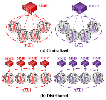
Figure 1: Graphical illustration of the centralized and distributed MME pooling scheme: (a) centralized MME pooling scheme; and (b) distributed MME pooling scheme

III-A Important Notations

Table I presents math and network notation that will be used throughout the paper. Table II lists notation related to the multi-objective particle swarm optimization algorithm. For any $\boldsymbol{N}\in\mathbb{N}$, $n\in\left[1,\boldsymbol{N}\right]$ indicates that $n$ is an integer number between 1 and $\boldsymbol{N}$. $z\in\left\{0,1\right\}$ denotes a binary number or more simple $z\in\mathbb{Z}$. Throughout the paper, $n\in\left[1,\boldsymbol{N}\right]$, $k\in\left[1,\boldsymbol{N}\right]$, $\boldsymbol{l}\in\left[1,\boldsymbol{L}\right]$, $t\in\left[1,\boldsymbol{\mathcal{T}}\right]$, $j=\left[1,\boldsymbol{\mathcal{P}}\right]$, and $i\in\left[1,\boldsymbol{\mathcal{N}}\right]$. Also, $\overline{{\rm rand}}\in\mathbb{R}$ and $\overline{{\rm rand}}\in\left[0,1\right]$.

TABLE I: Math and Network Notation

$\mathbb{R}^{n\times m}$	:	Real $n\times m$ dimensional matrix
$\mathbb{Z}^{n\times m}$	:	Binary $n\times m$ dimensional matrix
$\mathbb{N}$	:	Set of integer numbers
⊤	:	Transpose of a component
$\boldsymbol{N}$	:	Number of cells within a list, $\boldsymbol{N}\in\mathbb{N}$
$\boldsymbol{L}$	:	Total number of lists, $\boldsymbol{L}\in\mathbb{N}$
$\boldsymbol{l}$	:	A single list between $1$ and $\boldsymbol{L}$, $\boldsymbol{l}\in\left[1,\boldsymbol{L}\right]$
$\overline{\mathbf{MX}}$	:	Maximum number of TAs assigned to list $\boldsymbol{l}$
$\mathbf{H}^{{\rm C}}$	:	MME cost relocation over handover process
$\overline{\mathbf{Prob}}_{k,n}$	:	Probability of a user to move to cell $n$ from cell $k$
$\mathbf{G}^{{\rm a}}$	:	Arrival rate of paging
$\mathbf{G}^{{\rm C}}$	:	Paging cost of equipment of a particular user
$\mathbf{G}_{k}^{{\rm T}}$	:	Total paging cost of cell $k$
$\mathbf{U}^{{\rm C}}$	:	TAU cost of UE moving from one list to another list
$\mathbf{U}_{k}^{{\rm T}}$	:	Total signaling cost of TAU of cell $k$
$\overline{\mathbf{UE}}_{k}$	:	Total number of UEs served by cell $k$
$\overline{\mathbf{GU}}_{k}^{{\rm T}}$	:	Total TAU and paging overhead of cell $k$
$\overline{\mathbf{HC}}_{k}^{\boldsymbol{l}}$	:	Inter-list handover rate of user(s) in cell $k$
$\mathbf{O}_{{\rm M}}^{\boldsymbol{l}}$	$=$	$\left\{\begin{array}[]{rl}1,&\text{if list $\boldsymbol{l}$ belongs to MME $M$,}\\ 0,&\text{otherwise}\end{array}\right.$
$\mathbf{Q}_{k}^{{\rm TA}}$	$=$	$\left\{\begin{array}[]{rl}1,&\text{if cell $k$ belongs to TA,}\\ 0,&\text{otherwise}\end{array}\right.$
$\sigma_{k}^{\boldsymbol{l}}$	:	Percentage of usage of list $\boldsymbol{l}$ associated with cell $k$
${\rm C}_{k,n}^{\boldsymbol{l}}$	$=$	$\left\{\begin{array}[]{rl}1,&\text{if cells $k$ and $n$ belong to $\boldsymbol{l}$,}\\ 0,&\text{otherwise}\end{array}\right.$

TABLE II: MOPSO Notation

$x_{i,j}$	:	Position of parameter $j$ within particle $i$, $\forall i,j\in\mathbb{N}$
$v_{i,j}$	:	Velocity of parameter $j$ within particle $i$, $\forall i,j\in\mathbb{N}$
$\mathcal{X}_{i}$	:	Candidate solution of particle $i$, $\forall i,j\in\mathbb{N}$
$\mathcal{V}_{i}$	:	Velocity of particle $i$, $\forall i\in\mathbb{N}$
$x_{i,j}^{\star}$	:	$j$th parameter of $i$th best local particle, $\forall i,j\in\mathbb{N}$
$x_{i,j}^{\star\star}$	:	$j$th parameter of $i$th best global particle, $\forall i,j\in\mathbb{N}$
$\boldsymbol{\mathcal{P}}$	:	Number of parameters within 1 particle, $\boldsymbol{\mathcal{P}}\in\mathbb{N}$
$\boldsymbol{\mathcal{N}}$	:	Number of particles within 1 population, $\boldsymbol{\mathcal{N}}\in\mathbb{N}$
$\boldsymbol{\mathcal{T}}$	:	Total number of iterations/generations, $\boldsymbol{\mathcal{T}}\in\mathbb{N}$
$t$	:	Iteration/generation number, $t\in\mathbb{N}$ , $t\in\left[1,\boldsymbol{\mathcal{T}}\right]$
$\alpha\left(t\right)$	:	Inertia factor at iteration/generation $t$, $\alpha\left(t\right)\in\mathbb{R}$
$\mathcal{S}_{i}^{\star}$	:	Non-dominated local set of $i$th particle, $\forall i\in\mathbb{N}$
$\mathcal{S}^{\star\star}$	:	Non-dominated global set
$\mathbf{S}^{{\rm L}}$	:	Size of non-dominated local set
$\mathbf{S}^{{\rm G}}$	:	Size of non-dominated global set
$\boldsymbol{\mathcal{J}}^{1}$	:	Objective function 1 to be minimized, $\boldsymbol{\mathcal{J}}^{1}\in\mathbb{R}$
$\boldsymbol{\mathcal{J}}^{2}$	:	Objective function 2 to be minimized, $\boldsymbol{\mathcal{J}}^{2}\in\mathbb{R}$
$\overline{{\rm rand}}$	:	A real random number between 0 and 1

III-B Preliminaries and Design Hypothesis

The cells are allocated within every TAL through the centralized MME pooling scheme. Every TA refers to a single cell, hence, TA and cell will be used interchangeably. The centralized MME pooling scheme is depicted in the upper portion of Figure 1. The model includes two layers of assignments. The first layer considers the Cells-to-TALs/MMEs assignment associated with the core network. The second layer presents the TALs/MMEs to UEs assignment, which relates to every cell within the system. The first layer of the system evaluates the UEs mobility pattern among the cells, then it allocates the cells in TALs/MMEs with the goal of attenuating the total signaling overhead caused by TAU and paging. In the second layer, a number of TALs is positioned at a portion of UEs termed $\sigma_{k}^{\boldsymbol{l}}$. The selection of $\sigma_{k}^{\boldsymbol{l}}$ defines the usage portion of every single TAL/MME per cell which leads to interference of TALs through the cells. This technique guarantees a broader assortment of cells in the list.

III-B1 Cell/TA-to-TAL/MME Assignment

The allocation of cell/TA-to-TAL/MME in the centralized pooling scheme is the main objective of the presented model. Every TAL refers to a certain one-to-one MME basis. The allocation of Cells-to-TAL/MME is given through a binary decision variable ${\rm C}_{k,n}^{\boldsymbol{l}}\in\mathbb{Z}$ for all $\boldsymbol{l},k,n\in\mathbb{N}$, $k,n\in\left[1,\boldsymbol{N}\right]$ and $\boldsymbol{l}\in\left[1,\boldsymbol{L}\right]$. In order to proceed with the model and problem formulation, it is necessary to present the following example.

Example 1.

As an illustrative example of ${\rm C}_{k,n}^{\boldsymbol{l}}\in\mathbb{Z}$ allocation in the search space, define ${\rm C}_{k,n}^{\boldsymbol{l}}$ to be a cell-to-TAL assignment. For one list ($\boldsymbol{l}=1$), define the maximum number of cells/TAs to be $\bar{\mathbf{n}}=3$ with $\boldsymbol{N}=4$ MMEs or lists. Accordingly, the total number of possible combinations in matrix $\bar{\boldsymbol{\mathcal{L}}}^{1}={\rm C}^{\boldsymbol{l}}$ is $3\times 4$, where ${\rm C}_{k,n}^{\boldsymbol{l}}$ is a binary decision created in the system. One can specify the decision variables in list 1 as

$$\bar{\boldsymbol{\mathcal{L}}}^{1} =\begin{bmatrix}1&0&1&1\\ 0&0&0&0\\ 1&0&1&1\\ 1&0&1&1\end{bmatrix}=\begin{bmatrix}{\rm C}_{1,1}^{1}&{\rm C}_{1,2}^{1}&{\rm C}_{1,3}^{1}&{\rm C}_{1,4}^{1}\\ {\rm C}_{2,1}^{1}&{\rm C}_{2,2}^{1}&{\rm C}_{2,3}^{1}&{\rm C}_{2,4}^{1}\\ {\rm C}_{3,1}^{1}&{\rm C}_{3,2}^{1}&{\rm C}_{3,3}^{1}&{\rm C}_{3,4}^{1}\\ {\rm C}_{4,1}^{1}&{\rm C}_{4,2}^{1}&{\rm C}_{4,3}^{1}&{\rm C}_{4,4}^{1}\end{bmatrix}$$ (1)

Equation (1) in Example 1 shows that $\bar{\boldsymbol{\mathcal{L}}}^{1}$is symmetric with $\bar{\boldsymbol{\mathcal{L}}}^{1}=\left(\bar{\boldsymbol{\mathcal{L}}}^{1}\right)^{\top}\in\mathbb{Z}^{4\times 4}$. Also, it demonstrates that number of nonzero rows/columns has to be 3. In addition, number of ones in any given nonzero row/column has to be 3 with one zero row/column. Therefore, a general cell-to-TAL assignment with $\boldsymbol{L}$ lists and $\boldsymbol{N}$ MMEs or lists can be expressed by

$$\bar{\boldsymbol{\mathcal{L}}}^{1} =\left[\begin{array}[]{c}\mathcal{L}_{1}^{1}\\ \mathcal{L}_{2}^{1}\\ \vdots\\ \mathcal{L}_{\boldsymbol{N}}^{1}\end{array}\right]=\begin{bmatrix}{\rm C}_{1,1}^{1}&{\rm C}_{1,2}^{1}&\dots&{\rm C}_{1,\boldsymbol{N}}^{1}\\ {\rm C}_{2,1}^{1}&{\rm C}_{2,2}^{1}&\dots&{\rm C}_{2,\boldsymbol{N}}^{1}\\ \vdots&\vdots&\ddots&\vdots\\ {\rm C}_{\boldsymbol{N},1}^{1}&{\rm C}_{\boldsymbol{N},2}^{1}&\dots&{\rm C}_{\boldsymbol{N},\boldsymbol{N}}^{1}\end{bmatrix}$$ (6)

$$\vdots\hskip 5.0pt =\hskip 10.00002pt\hskip 10.00002pt\vdots\hskip 10.00002pt\hskip 10.00002pt\hskip 10.00002pt\hskip 10.00002pt\hskip 10.00002pt\hskip 10.00002pt\hskip 10.00002pt\hskip 10.00002pt\vdots$$

$$\bar{\boldsymbol{\mathcal{L}}}^{\boldsymbol{L}} =\left[\begin{array}[]{c}\mathcal{L}_{1}^{\boldsymbol{L}}\\ \mathcal{L}_{2}^{\boldsymbol{L}}\\ \vdots\\ \mathcal{L}_{\boldsymbol{N}}^{\boldsymbol{L}}\end{array}\right]=\begin{bmatrix}{\rm C}_{1,1}^{\boldsymbol{L}}&{\rm C}_{1,2}^{\boldsymbol{L}}&\dots&{\rm C}_{1,\boldsymbol{N}}^{\boldsymbol{L}}\\ {\rm C}_{2,1}^{\boldsymbol{L}}&{\rm C}_{2,2}^{\boldsymbol{L}}&\dots&{\rm C}_{2,\boldsymbol{N}}^{\boldsymbol{L}}\\ \vdots&\vdots&\ddots&\vdots\\ {\rm C}_{\boldsymbol{N},1}^{\boldsymbol{L}}&{\rm C}_{\boldsymbol{N},2}^{\boldsymbol{L}}&\dots&{\rm C}_{\boldsymbol{N},\boldsymbol{N}}^{\boldsymbol{L}}\end{bmatrix}$$ (11)

The assignment of the maximum number of cells within a list has to satisfy the following expression

$$\sum\limits_{k=1}^{\boldsymbol{N}}\sum\limits_{n,n\neq k}^{\boldsymbol{N}}{\rm C}_{k,n}^{\boldsymbol{l}}\leqslant\overline{\mathbf{MX}},\hskip 10.00002pt\forall\boldsymbol{l}\in\left[1,\boldsymbol{L}\right]$$ (12)

where $\overline{\mathbf{MX}}$ denotes maximum number of TAs in a list. Also, according to the above-mentioned discussion and Example 1, the cell/TA assignment in every TAL takes the following form

$${\rm C}_{k,n}^{\boldsymbol{l}}={\rm C}_{n,k}^{\boldsymbol{l}},\hskip 10.00002pt\forall\boldsymbol{l}\in[1,\boldsymbol{L}],\text{ and }k,n,k\neq n\in\left[1,\boldsymbol{N}\right]$$ (13)

III-B2 TAL-to-UE

According to the fact that any TAL associated with MME could be assigned to more than one cell, the assigned cell has not to violate the MME load of any nonzero $n$ column, which could be achieved by

$$\sum\limits_{k=1}^{\boldsymbol{N}}\sigma_{k}^{\boldsymbol{l}}\cdot{\rm C}_{k,n}^{\boldsymbol{l}}=1,\hskip 10.00002pt\forall\>\boldsymbol{l}\in\left[1,\boldsymbol{L}\right]$$ (14)

where $\sigma_{k}^{\boldsymbol{l}}$ denotes the percentage of usage of list $\boldsymbol{l}$ associated with cell $k$.

III-C Total Signaling of TAU and paging

The signaling cost of TAU and paging is a fundamental consideration when placing an idle-user in a cellular network [11, 13]. In fact, the total signaling overhead created by TAU is a result of a user movement from a cell in one TAL to a different TAL. Whereas, the total signaling overhead created by paging is due to a necessity to locate a user via the core network. Since the total signaling overhead cost is inversely related to the size of TAL, there is negative correlation between the total signaling created by TAU and paging, and the size of TAL. This is the case due to the fact that the greater the number of cells within a certain list the lower is the probability for a user to move between lists.

III-D Problem Description and Cost Functions

This subsection presents the centralized MME pooling problem [5, 14, 6]. The objective is to minimize the signaling overhead, which can be accomplished by minimizing two objective functions, namely, the total signaling cost of TAU and paging, and the total inter-list handover. The total signaling cost of TAU of cell $k$ for any $n$ nonzero column is equivalent to

$$\begin{split}\mathbf{U}_{k}^{{\rm T}}=&\overline{\mathbf{UE}}_{k}\cdot\overline{\mathbf{Prob}}_{k,n}\cdot\mathbf{U}^{{\rm C}}\cdot\left[\sum\limits_{\boldsymbol{l}=1}^{\boldsymbol{L}}\mathbf{H}^{{\rm C}}\cdot\mathbf{O}_{{\rm M}}^{\boldsymbol{l}}\cdot\sigma_{k}^{\boldsymbol{l}}\left(1-{\rm C}_{k,n}^{\boldsymbol{l}}\right)\right],\\ &\hskip 9.00002pt\forall\>k,n,k\neq n\in\left[1,\boldsymbol{N}\right]\end{split}$$ (15)

with $\overline{\mathbf{UE}}_{k}$ being the total number of UEs served by cell $k$, $\mathbf{U}^{{\rm C}}$ being the TAU cost of UE moving from one list to another, $\mathbf{H}^{{\rm C}}$ being the MME cost relocation over handover process, and $\mathbf{O}_{{\rm M}}^{\boldsymbol{l}}$ defining whether list $\boldsymbol{l}$ belongs to MME $M$ or not. The total cost of paging of cell $k$ for any $n$ nonzero column can be evaluated by

$$\begin{split}\mathbf{G}_{k}^{{\rm T}}=&\mathbf{G}^{{\rm a}}\cdot\mathbf{G}^{{\rm C}}\cdot\left[\sum\limits_{\boldsymbol{l}=1}^{\boldsymbol{L}}\overline{\mathbf{UE}}_{k}\cdot\sigma_{k}^{\boldsymbol{l}}+\sum\limits_{\boldsymbol{l}=1}^{\boldsymbol{L}}\sum\limits_{n,k\neq n}^{\boldsymbol{N}}\overline{\mathbf{UE}}_{n}\cdot{\rm C}_{k,n}^{\boldsymbol{l}}\cdot\sigma_{n}^{\boldsymbol{l}}\right]\\ &\hskip 40.00006pt\hskip 10.00002pt\forall\>k\in\left[1,\boldsymbol{N}\right]\end{split}$$ (16)

where $\mathbf{G}^{{\rm a}}$ denotes the arrival rate of paging and $\mathbf{G}^{{\rm C}}$ refers to the paging cost of equipment of a particular user. Recall the constraints in Equations (11), (12), (13), and (14)

$$\sum\limits_{k=1}^{\boldsymbol{N}}\sigma_{k}^{\boldsymbol{l}}\cdot{\rm C}_{k,n}^{\boldsymbol{l}}=1,\hskip 10.00002pt\forall\>\boldsymbol{l}\in\left[1,\boldsymbol{L}\right]$$ (17)

$$\sum\limits_{k,n,k\neq n}^{\boldsymbol{N}}{\rm C}_{k,n}^{\boldsymbol{l}}\leqslant\overline{\mathbf{MX}},\hskip 10.00002pt\forall\>\boldsymbol{l}\in\left[1,\boldsymbol{L}\right]$$ (18)

$${\rm C}_{k,n}^{\boldsymbol{l}}={\rm C}_{n,k}^{\boldsymbol{l}},\hskip 10.00002pt\forall\boldsymbol{l}\in[1,\boldsymbol{L}],\>k,n,k\neq n\in\left[1,\boldsymbol{N}\right]$$ (19)

$$0\leq\sigma_{k}^{\boldsymbol{l}}\leq 1$$ (20)

$$\mathbf{O}_{{\rm M}}^{\boldsymbol{l}}\in\left\{0,1\right\}$$ (21)

$${\rm C}_{k,n}^{\boldsymbol{l}}\in\left\{0,1\right\}$$ (22)

where Equations (20), (21), and (22) refer to boundary constraints. Accordingly, the total signaling cost of TAU and paging of the $i$th element is defined by

$$\overline{\mathbf{GU}}_{k}^{{\rm T}}=\mathbf{G}_{k}^{{\rm T}}+\mathbf{U}_{k}^{{\rm T}},\hskip 10.00002pt\forall\>k\in\left[1,\boldsymbol{N}\right],k\in\mathbb{N}$$ (23)

and the first objective function is given by

$$\boldsymbol{\mathcal{J}}^{1}=\sum\limits_{k=1}^{\boldsymbol{N}}\overline{\mathbf{GU}}_{k}^{{\rm T}}$$ (24)

Hence, the total signaling overhead introduced by TAU and paging could be minimized through the minimization of $\boldsymbol{\mathcal{J}}^{1}$ in Equation (24). On the other side, the total inter-list handover of the $k$th element for any $n$ nonzero column is

$$\overline{\mathbf{HC}}_{k}^{\boldsymbol{l}}=\sum\limits_{\boldsymbol{l}=1}^{\boldsymbol{L}}\overline{\mathbf{UE}}_{k}\cdot\overline{\mathbf{Prob}}_{k,n}\cdot\left(1-{\rm C}_{k,n}^{\boldsymbol{l}}\right)$$ (25)

with the second objective function being defined by

$$\boldsymbol{\mathcal{J}}^{2}=\sum\limits_{k=1}^{\boldsymbol{N}}\overline{\mathbf{HC}}_{k}^{\boldsymbol{l}}$$ (26)

such that the minimization of total signaling overhead could be achieved by diminishing the total inter-MME reallocation cost, which is defined by $\boldsymbol{\mathcal{J}}^{2}$ in Equation (26). The fluid flow model is popular and frequently employed to resemble the mobility behavior of a user in a system [5]. The fluid flow model presents the UEs traffic outflow rate of an enclosed area. In this specific case enclosed area refers to a single cell. For a given cell $k$, let $\overline{PM}$ denote its perimeter, $\rho_{k}$ refer to UE density of the cell, and $v$ be the UE average velocity. Hence, the average of cell crossings with respect to time is defined by

$$\dfrac{\rho_{k}\cdot\overline{PM}\cdot v}{\pi}$$ (27)

implying that the cells are hexagonal-shaped with length $L^{{\rm H}}$, which means that $\overline{PM}=6L^{{\rm H}}$.

According to the above-mentioned discussion and the problem statement, the two objectives $\boldsymbol{\mathcal{J}}^{1}$ and $\boldsymbol{\mathcal{J}}^{2}$ are inversely related. A weighting scheme can be applied to the two conflicting objectives [24]. However, there is no guarantee that the obtained solution would be the best compromise solution [28].

III-E Overview of model decomposition using MINLP

The problem formulation of the model mentioned above is NP-hard, thus, the problem can be divided into two sub-problems. One sub-problem may consider the cell-to-TAL/MME assignment which is allocated periodically to minimize the inter-list handover rate of UEs from one cell to another. This sub-problem mainly includes Equations (18), (19), (25) and (26). The second sub-problem could assume the set of TALs/MMEs given and, thereby, using the given data one can find the optimum usage ratio for each TAL/MME. The other sub-problem mainly includes Equations (20), (22), (15), (16), (23) and (24). For a full description of the previously mentioned two sub-problems using MINLP visit [7, 6]. A scrutiny look at the final solution obtained by MINLP, one can find that the solution is confined on the Pareto-optimal front. However, one objective is strictly favored the optimum solution over the other one, which is a significant weakness. Thus, the best compromise solution cannot be achieved using this method. Consequently, a random artificial search technique such as optimization algorithms based on the social behavior of animals could help in approaching a set of solutions on the Pareto-optimal of the NP-hard problem [36]. In that case, the two above-mentioned sub-problems would be solved simultaneously through the optimization algorithm and the best compromise solution would be defined.

IV Multi-objective Particle Swarm Optimization

IV-A Particle Swarm Optimization

Particle Swarm Optimization (PSO) is considered to be an evolutionary heuristic technique. This technique imitates the cognitive and social behavior of animals in their natural environment such as fish schooling and bird swarming [20, 25]. In the very beginning, PSO is initiated by releasing an initial random population of particles into the space. In this paper, the population size is fixed. Every particle within the space is a potential solution or, in other words, a potential candidate. It is worth mentioning that particle and candidate will be used interchangeably. Each single particle has a set of parameters such that the set of parameters swarms in the space irregularly in a multi-dimensional space. The swarming of particles is aimed at determining an optimal solution. The position of a particle represents a possible solution including the optimal solution. The velocity of every particle has a major impact of heading the best potential solution or alternatively, the best candidate position. Additionally, the subsequent position and velocity of each particle depend on: current velocity, current position, current position of the neighboring particles, and best position of the neighboring particles. Let $\boldsymbol{\mathcal{P}}\in\mathbb{N}$ and $\boldsymbol{\mathcal{N}}\in\mathbb{N}$ denote number of parameters to be optimized and population size, respectively. For any $i$th candidate solution within the space, define the candidate solution (position) at iteration $t\in\mathbb{N}$ by $\mathcal{X}_{i}=\left[x_{i,1}\left(t\right),\ldots,x_{i,\boldsymbol{\mathcal{P}}}\left(t\right)\right]^{\top}\in\mathbb{R}^{\boldsymbol{\mathcal{P}}}$ and the velocity of every candidate by $\mathcal{V}_{i}=\left[v_{i,1}\left(t\right),\ldots,v_{i,\boldsymbol{\mathcal{P}}}\left(t\right)\right]^{\top}\in\mathbb{R}^{\boldsymbol{\mathcal{P}}}$ for all $t=1,2,\ldots,\boldsymbol{\mathcal{T}}$ and $i=1,2,\ldots,\boldsymbol{\mathcal{N}}$. Accordingly, the velocity update of the $j$th parameter within the $i$th swarming particle is given by [20, 25]

$$\begin{split}v_{i,j}\left(t\right)=&\alpha\left(t\right)v_{i,j}\left(t-1\right)\\ &+k_{1}\overline{{\rm rand}}_{1}\left(x_{i,j}^{\star}\left(t-1\right)-x_{i,j}\left(t-1\right)\right)\\ &+k_{2}\overline{{\rm rand}}_{2}\left(x_{i,j}^{\star\star}\left(t-1\right)-x_{i,j}\left(t-1\right)\right)\end{split}$$ (28)

where $\alpha\left(t\right)$ denotes an inertial factor to be continuously reduced with every iteration such that $\alpha\left(t\right)=0.99\alpha\left(t-1\right)$, $\overline{{\rm rand}}_{1}$ and $\overline{{\rm rand}}_{2}$ are real random numbers between 0 and 1. $k_{1}$ and $k_{2}$ refer to weighting factors associated with personal and social influence, respectively. $x_{i,j}^{\star}$ denotes a best local particle within the previous generation while $x_{i,j}^{\star\star}$ refers to the best global particle within all previous generations, for all $i=1,2,\ldots,\boldsymbol{\mathcal{N}}$ and $j=1,2,\ldots,\boldsymbol{\mathcal{P}}$. It should be noted that the iterative solution starts at $t=1$ continues until the total number of iterations set by the user is reached. The position update of a parameter within the swarming particle associated with Equation (28) can be expressed by [20, 25]

$$x_{i,j}\left(t\right)=v_{i,j}\left(t\right)+x_{i,j}\left(t-1\right)$$ (29)

The candidate solution $\mathcal{X}_{i}$ is initialized between the minimum and maximum boundaries of the space, termed $x_{{\rm min}}$ and $x_{{\rm max}}$, respectively, such that $x_{i,j}\left(t\right)\in\left[x_{{\rm min}}^{j},x_{{\rm max}}^{j}\right]$. On the other side, the velocity $v_{i,j}\left(t\right)$ is initiated to be $v_{i,j}\left(t\right)\in\left[-v_{{\rm max}}^{j},v_{{\rm max}}^{j}\right]$, while $v_{{\rm max}}$ is given by

$$v_{{\rm max}}=\frac{x_{{\rm max}}-x_{{\rm min}}}{N_{{\rm intv}}}$$ (30)

with $N_{{\rm intv}}$ being the number of intervals.

IV-B Pareto-optimal front and clustering

For a multi-objective optimization problem, or to be more specific, two-objective optimization problem, the trade-off between any two solutions can follow two possible scenarios: either one dominates the other or none dominates the other. For instance, if $\mathcal{X}_{1}$ dominates $\mathcal{X}_{2}$ according to the first objective, while $\mathcal{X}_{2}$ dominates $\mathcal{X}_{1}$ based on the second objective, both solutions are considered non-dominated and are located on the Pareto-optimal front. All the solution positioned on the Pareto-optimal front are combined into one set. Number of solutions on the Pareto-optimal front could be extremely large. Clustering, however, can reduce the number of non-dominated solutions within a large set while keeping the desired characteristics of the trade-off. In MOPSO, the local set of non-dominated solutions is denoted by $\mathcal{S}^{\star}$ with $\mathcal{S}_{i}^{\star}=\mathcal{X}_{i}\left(1\right)$. After which, non-dominated solutions are to be added to form a large set $\mathcal{S}_{i}^{\star}$. Clustering is performed based on the distance between two pairs. The pairs separated by large distance are retained while minimal distance pairs are combined into one cluster [37]. Therefore, the local non-dominated set can be resized to satisfy the user settings, for instance $\mathcal{S}_{i}^{\star}$, has the size $\mathbf{S}^{{\rm L}}$. The non-dominated global set is denoted by $\mathcal{S}^{\star\star}$ and includes all the non-dominated solutions from the first to the last generation. In the same spirit, clustering is performed to keep pairs within large distance and combine pairs within small distance. In that case, the non-dominated global set will not exceed a predefined size, for example $\mathcal{S}^{\star\star}$ has the size $\mathbf{S}^{{\rm G}}$. It should be remarked that $\mathcal{X}_{i}^{\star}$ and $\mathcal{X}_{k}^{\star\star}$ belong to the sets $\mathcal{S}_{i}^{\star}$ and $\mathcal{S}^{\star\star}$, respectively. The steps of the clustering algorithm can be found in [8, 26].

Individual distances between all the members of the local set $\mathcal{S}_{i}^{\star}$, and the members of the global set $\mathcal{S}^{\star\star}$ are measured with respect to the objective space. Let $\mathcal{X}_{i}^{\star}$ and $\mathcal{X}_{i}^{\star\star}$ denote members of $\mathcal{S}_{i}^{\star}$ and $\mathcal{S}^{\star\star}$, respectively. For the case when $\mathcal{X}_{i}^{\star}$ and $\mathcal{X}_{i}^{\star\star}$ give minimum distances, they are to be selected as local best and global best of the $i$th particle, respectively.

IV-C Extraction of the best compromise solution

Once the Pareto-optimal front is available, one solution should be selected as the best compromise solution. The fuzzy approach is implemented to identify the best compromise solution. Define $M$ as a number of non-dominated objectives on the Pareto-optimal front and $N^{{\rm Obj}}$ as a number of objectives. Let the set of objective functions on the Pareto-optimal front be $\bar{\boldsymbol{\mathcal{J}}}^{c}=\left[\bar{\boldsymbol{\mathcal{J}}}_{1}^{c},\bar{\boldsymbol{\mathcal{J}}}_{2}^{c},\ldots,\bar{\boldsymbol{\mathcal{J}}}_{M}^{c}\right]\in\mathbb{R}^{M}$ with $\bar{\boldsymbol{\mathcal{J}}}_{{\rm min}}^{c}$ and $\bar{\boldsymbol{\mathcal{J}}}_{{\rm max}}^{c}$ being minimum and maximum objective functions of $\bar{\boldsymbol{\mathcal{J}}}^{c}$, respectively, for all $c=1,2,\ldots,N^{{\rm Obj}}$ and for $m=1,2,\ldots,M$. The first step is to obtain the membership function $\mu_{m}^{c}$ such that

$$\mu_{m}^{c}=\left\{\begin{array}[]{cc}1&\bar{\boldsymbol{\mathcal{J}}}_{m}^{c}\leq\bar{\boldsymbol{\mathcal{J}}}_{{\rm min}}^{c}\\ \frac{\bar{\boldsymbol{\mathcal{J}}}_{{\rm max}}^{c}-\bar{\boldsymbol{\mathcal{J}}}_{m}^{c}}{\bar{\boldsymbol{\mathcal{J}}}_{{\rm max}}^{c}-\bar{\boldsymbol{\mathcal{J}}}_{{\rm min}}^{c}}&\text{otherwise}\\ 0&\bar{\boldsymbol{\mathcal{J}}}_{m}^{c}\geq\bar{\boldsymbol{\mathcal{J}}}_{{\rm max}}^{c}\end{array}\right.$$ (31)

for $m=1,2,\ldots,M$, and $c=1,2,\ldots,N^{{\rm Obj}}$. In our case there are two objectives, thus $N^{{\rm Obj}}=2$. Next, the best compromise solution is obtained by

$$\bar{\mu}_{m}=\frac{\sum_{c=1}^{N^{{\rm Obj}}}\mu_{m}^{c}}{\sum_{m=1}^{M}\sum_{c=1}^{N^{{\rm Obj}}}\mu_{m}^{c}}$$ (32)

Given the solution of $\bar{\mu}_{m}$ as in Equation (32) for $m=1,2,\ldots,M$, the best compromise solution is $\bar{\mu}_{m}$ that has the maximum value. Figure 2 illustrates the flow chart of MOPSO computational algorithm.

Figure 2: The computational flowchart of MOPSO [8].

IV-D Implementation of the MOPSO algorithm

For simplicity, the implementation process of the MOPSO algorithm can be subdivided into two stages:

Stage I: Recall Cell/TA-to-TAL/MME Assignment in Section III, specifically Equations (11), (12) and (13). There are $\boldsymbol{N}\in\mathbb{N}$ cells in the system with $\bar{\mathbf{n}}\in\left[1,\boldsymbol{N}\right)$ cells being distributed within the list and $\bar{\mathbf{n}}<\boldsymbol{N}$:

$$\bar{\boldsymbol{\mathcal{L}}}^{1} =\left[\begin{array}[]{c}\mathcal{L}_{1}^{1}\\ \vdots\\ \mathcal{L}_{\boldsymbol{N}}^{1}\end{array}\right]=\left[\begin{array}[]{ccc}{\rm C}_{1,1}^{1}&\cdots&{\rm C}_{1,\boldsymbol{N}}^{1}\\ \vdots&\ddots&\vdots\\ {\rm C}_{\boldsymbol{N},1}^{1}&\cdots&{\rm C}_{\boldsymbol{N},\boldsymbol{N}}^{1}\end{array}\right]\in\mathbb{Z}^{\boldsymbol{N}\times\boldsymbol{N}}$$ (39)

$$\vdots\hskip 5.0pt =\hskip 10.00002pt\hskip 10.00002pt\vdots\hskip 10.00002pt\hskip 10.00002pt\hskip 10.00002pt\hskip 10.00002pt\hskip 10.00002pt\hskip 10.00002pt\hskip 10.00002pt\hskip 10.00002pt\hskip 10.00002pt\hskip 10.00002pt\vdots$$

$$\bar{\boldsymbol{\mathcal{L}}}^{\boldsymbol{L}} =\left[\begin{array}[]{c}\mathcal{L}_{1}^{\boldsymbol{L}}\\ \vdots\\ \mathcal{L}_{\boldsymbol{N}}^{\boldsymbol{L}}\end{array}\right]=\left[\begin{array}[]{ccc}{\rm C}_{1,1}^{\boldsymbol{L}}&\cdots&{\rm C}_{1,\boldsymbol{N}}^{\boldsymbol{L}}\\ \vdots&\ddots&\vdots\\ {\rm C}_{\boldsymbol{N},1}^{\boldsymbol{L}}&\cdots&{\rm C}_{\boldsymbol{N},\boldsymbol{N}}^{\boldsymbol{L}}\end{array}\right]\in\mathbb{Z}^{\boldsymbol{N}\times\boldsymbol{N}}$$ (46)

such that $\bar{\boldsymbol{\mathcal{L}}}\in\mathbb{Z}^{\boldsymbol{L}\boldsymbol{N}\times\boldsymbol{N}}$ denotes all lists and the associated superscript refers to the list number. Thus, the number of the cell-to-TAL combination is given by $\boldsymbol{L}\times\boldsymbol{N}$. It should be noted that $\bar{\boldsymbol{\mathcal{L}}}^{\boldsymbol{l}}$ is a symmetric matrix for $\boldsymbol{l}=1,2,\ldots,\boldsymbol{L}$, such that $\bar{\boldsymbol{\mathcal{L}}}^{\boldsymbol{l}}=\left(\bar{\boldsymbol{\mathcal{L}}}^{\boldsymbol{l}}\right)^{\top}\in\mathbb{Z}^{\boldsymbol{N}\times\boldsymbol{N}}$, with ^⊤ being the transpose of the matrix. There are $\bar{\mathbf{n}}$ nonzero rows within $\bar{\boldsymbol{\mathcal{L}}}^{\boldsymbol{l}}$ and the rest of rows ($\boldsymbol{N}-\bar{\mathbf{n}}$) are equal to zero, while the dimension of each row is $1\times\boldsymbol{N}$. Let $\mathcal{L}_{\star_{\boldsymbol{l}}}^{\boldsymbol{l}}\in\mathbb{Z}^{1\times\boldsymbol{N}}$ be a nonzero row, such that $\star_{\boldsymbol{l}}$ is an integer between 1 and $\boldsymbol{N}$ ($\star_{\boldsymbol{l}}\in\mathbb{N}$ and $\star_{\boldsymbol{l}}\in[1,\mathbf{N}]$). In fact, $\bar{\mathbf{n}}$ numbers within $\mathcal{L}_{\star_{\boldsymbol{l}}}^{\boldsymbol{l}}$ are equal to 1 and the rest are zeros. Also, $\bar{\mathbf{n}}$ nonzero columns within the square matrix $\bar{\boldsymbol{\mathcal{L}}}^{\boldsymbol{l}}$ are identical, for $\boldsymbol{l}=1,2,\ldots,\boldsymbol{L}$. Accordingly, number of variables to be optimized and allocated within one list is $\boldsymbol{N}$. In the $\boldsymbol{L}$ lists in Equation (46), there are $\boldsymbol{L}\times\boldsymbol{N}$ binary parameters to be optimized and subsequently allocated such that

$$\mathbf{X}^{1}=\left[\begin{array}[]{cccc}\mathcal{L}_{\star_{1}}^{1}&\mathcal{L}_{\star_{2}}^{2}&\cdots&\mathcal{L}_{\star_{L}}^{\boldsymbol{L}}\end{array}\right]^{\top}\in\mathbb{Z}^{\boldsymbol{L}\boldsymbol{N}\times 1}$$ (47)

Stage II: Consider TAL-to-UE in Section III, Equation (14). Each TAL is associated with a specific MME and their relationship can be expressed as

$$\sum\limits_{k=1}^{\boldsymbol{N}}\sigma_{k}^{\boldsymbol{l}}\cdot{\rm C}_{k,n}^{\boldsymbol{l}} =1,\hskip 10.00002pt\boldsymbol{l}=1,2,\ldots,\boldsymbol{L}$$ (48)

with $\sigma^{\boldsymbol{l}}=\left[\begin{array}[]{cccc}\sigma_{1}^{\boldsymbol{l}}&\sigma_{2}^{\boldsymbol{l}}&\cdots&\sigma_{\boldsymbol{N}}^{\boldsymbol{l}}\end{array}\right]\in\mathbb{R}^{1\times\boldsymbol{N}}$ for $\boldsymbol{l}=1,2,\ldots,10$. Therefore, in the $\boldsymbol{L}$ lists in Equation (48), there are another $\boldsymbol{L}\times\boldsymbol{N}$ real parameters to be optimized. The decision variable $\sigma^{\boldsymbol{l}}$ has to match the $\mathcal{L}_{\star_{\boldsymbol{l}}}^{\boldsymbol{l}}$, for instance

$$\sigma_{k}^{\boldsymbol{l}}=\begin{cases}0,&\text{if }{\rm C}_{\star_{\boldsymbol{l}},k}^{\boldsymbol{l}}=0\\ \sigma_{k}^{\boldsymbol{l}},&\text{if }{\rm C}_{\star_{\boldsymbol{l}},k}^{\boldsymbol{l}}=1\end{cases}$$ (49)

In order to obtain $\sigma^{\boldsymbol{l}}$, define the following auxiliary variable $\bar{\sigma}^{\boldsymbol{l}}=\left[\begin{array}[]{cccc}\bar{\sigma}_{1}^{\boldsymbol{l}}&\bar{\sigma}_{2}^{\boldsymbol{l}}&\cdots&\bar{\sigma}_{\boldsymbol{N}}^{\boldsymbol{l}}\end{array}\right]\in\mathbb{R}^{1\times\boldsymbol{N}}$ with $\bar{\sigma}_{k}^{\boldsymbol{l}}\in\left[0,1\right]$ for all $\boldsymbol{l}=1,2,\ldots,10$ and $k=1,2,\ldots,\boldsymbol{N}$. Hence, we optimize for $\mathbf{X}^{2}$ such that

$$\mathbf{X}^{2}=\left[\begin{array}[]{cccc}\bar{\sigma}^{1}&\bar{\sigma}^{2}&\cdots&\bar{\sigma}^{\boldsymbol{N}}\end{array}\right]^{\top}\in\mathbb{R}^{\boldsymbol{L}\boldsymbol{N}\times 1}$$ (50)

After optimizing $\mathbf{X}^{2},$ $\sigma^{\boldsymbol{l}}$ can be defined as follows

$$\sigma_{k}^{\boldsymbol{l}}=\begin{cases}0,&\text{if }{\rm C}_{\star_{\boldsymbol{l}},k}^{\boldsymbol{l}}=0\\ \bar{\sigma}_{k}^{\boldsymbol{l}},&\text{if }{\rm C}_{\star_{\boldsymbol{l}},k}^{\boldsymbol{l}}=1\end{cases}$$ (51)

where ${\rm C}_{\star_{\boldsymbol{l}},k}^{1}$ is a cell associated with the nonzero row $\mathcal{L}_{\star_{\boldsymbol{l}}}^{\boldsymbol{l}}$. Next, to satisfy the equality in Equation (48), one has

$$\sigma^{\boldsymbol{l}}=\frac{\sigma^{\boldsymbol{l}}}{\sum\limits_{i=1}^{\boldsymbol{N}}\sigma_{k}^{\boldsymbol{l}}}$$ (52)

This concludes the implementation process of the MOPSO algorithm.

Therefore, Stage I and Stage II summarize the optimization process and number of parameters to be optimized. It is worth re-mentioning that $\mathbf{X}^{1}$ and $\mathbf{X}^{2}$ in Stage I and Stage II, respectively, would be solved by MOPSO algorithm simultaneously. In total, there are $2\boldsymbol{L}\boldsymbol{N}$ parameters to be optimized. Let $\mathcal{X}_{i}$ denote the vector of parameters to be optimized with dimension $2\boldsymbol{L}\boldsymbol{N}\times 1$ for all $i=1,2,\ldots,\boldsymbol{\mathcal{N}}$. One can find the complete vector ($\mathcal{X}_{i}$) to be

$$\mathcal{X}_{i}=\left[\begin{array}[]{c}\mathbf{X}^{1}\\ \mathbf{X}^{2}\end{array}\right]=\left[x_{i,1},\ldots,x_{i,\boldsymbol{\mathcal{P}}}\right]^{\top}$$ (53)

The total number of parameters to be optimized in one particle is $\boldsymbol{\mathcal{P}}=2\boldsymbol{L}\boldsymbol{N}$ with $\mathbf{X}^{1}\in\mathbb{Z}^{\boldsymbol{N}\times 1}$ and $\mathbf{X}^{2}\in\mathbb{R}^{\boldsymbol{N}\times 1}$.

A set of random particles is initiated such that every single particle has $\boldsymbol{\mathcal{P}}=2\boldsymbol{L}\boldsymbol{N}$ parameters, and there are $\boldsymbol{\mathcal{N}}$ particles within one iteration/generation. Therefore, the number of objective functions obtained from one generation is $2\boldsymbol{L}\boldsymbol{N}$. Velocity and position of the $i$th particle are defied according to Equations (28) and (29), respectively. All the remaining steps are detailed above.

IV-E Computational flow using MOPSO

The computational flow of the proposed location management of LTE networks using MOPSO technique can be briefly summarized as follows:

Step 1 (Initialization): initiate $t=1$ and generate $\boldsymbol{\mathcal{N}}$ random particles $\mathcal{X}_{i}\left(1\right)\in\mathbb{R}^{\boldsymbol{\mathcal{P}}}\forall i=1,2,\ldots,\boldsymbol{\mathcal{N}}$ where $\mathcal{X}_{i}\left(1\right)=\left[\mathbf{X}^{1^{\top}},\mathbf{X}^{2^{\top}}\right]^{\top}=\left[x_{i,1}\left(1\right),\ldots,x_{i,\boldsymbol{\mathcal{P}}}\left(1\right)\right]^{\top}\in\mathbb{R}^{\boldsymbol{\mathcal{P}}}$ such that $\mathbf{X}^{1}\in\mathbb{Z}^{\boldsymbol{N}\times 1}$, $\mathbf{X}^{2}\in\mathbb{R}^{\boldsymbol{N}\times 1}$, and $x_{i,k}\left(1\right)\in\left[x_{{\rm min}}^{k},x_{{\rm max}}^{k}\right]$. Likewise, generate $\boldsymbol{\mathcal{N}}$ random initial velocities $\mathcal{V}_{i}\left(1\right)\in\mathbb{R}^{\boldsymbol{\mathcal{P}}}\forall i=1,2,\ldots,\boldsymbol{\mathcal{N}}$ where $\mathcal{V}_{i}\left(1\right)=\left[v_{i,1}\left(1\right),\ldots,v_{i,\boldsymbol{\mathcal{P}}}\left(1\right)\right]^{\top}$ and $v_{i,k}\left(1\right)\in\left[-v_{{\rm max}}^{k},v_{{\rm max}}^{k}\right]$. Evaluate the objective function of every particle. For every particle, generate a local best set $\mathcal{S}_{i}^{\star}\left(1\right)$ with $\mathcal{X}_{i}^{\star}\left(1\right)=\mathcal{X}_{i}\left(1\right)$ and $\mathcal{S}_{i}^{\star}\left(1\right)=\mathcal{X}_{i}^{\star}\left(1\right)$ for all $i=1,2,\ldots,\boldsymbol{\mathcal{N}}$. Search for non-dominated solutions and generate a non-dominated global set $\mathcal{S}^{\star\star}\left(1\right)$ where the closest member of $\mathcal{S}^{\star\star}\left(1\right)$ to $\mathcal{X}_{i}^{\star}\left(1\right)$ is marked as the global best $\mathcal{X}_{i}^{\star\star}\left(1\right)$ of the $i$th particle. Set the initial value of the inertia factor $\alpha\left(1\right)$.

Step 2 (iteration update): update the iteration number to $t=t+1$.

Step 3 (Inertia factor update): update the inertia factor.

Step 4 (Velocity update): update the velocity $\mathcal{V}_{i}\left(t\right)$ as defined in Equation (28) given the particle $\mathcal{X}_{i}\left(t-1\right)$, the local best $\mathcal{X}_{i}^{\star}\left(t-1\right)$, and the global best $\mathcal{X}_{i}^{\star\star}\left(t-1\right)$ for all $i=1,2,\ldots,\boldsymbol{\mathcal{N}}$.

Step 5 (Position update): update the position $\mathcal{X}_{i}\left(t\right)$ in accordance with Equation (29) given the particle $\mathcal{X}_{i}\left(t-1\right)$ and the velocity $\mathcal{V}_{i}\left(t\right)$ for all $i=1,2,\ldots,\boldsymbol{\mathcal{N}}$.

Step 6 (Non-dominated local set update): The updated position $\mathcal{X}_{i}\left(t\right)$ is added to the set $\mathcal{S}_{i}^{\star}\left(t\right)$ for all $i=1,2,\ldots,\boldsymbol{\mathcal{N}}$. Keep all non-dominated solutions and eliminate all dominated solutions within the local best set $\mathcal{S}_{i}^{\star}\left(t\right)$. If the size of $\mathcal{S}_{i}^{\star}\left(t\right)$ exceeds the predefined value $\mathbf{S}^{{\rm L}}$, apply clustering and reduce the size to $\mathbf{S}^{{\rm L}}$.

Step 7 (Non-dominated global set update): Set $\mathcal{S}^{\star\star}\left(t\right)=\mathcal{S}^{\star\star}\left(t-1\right)$. If any of the non-dominated solutions within $\mathcal{S}_{i}^{\star}\left(t\right)$ are non-dominated by $\mathcal{S}^{\star\star}\left(t\right)$ and are not its members, add it to the set $\mathcal{S}^{\star\star}\left(t\right)$. If the size of $\mathcal{S}^{\star\star}\left(t\right)$ exceeds the predefined limit $\mathbf{S}^{{\rm G}}$, apply clustering to reduce the size to $\mathbf{S}^{{\rm G}}$.

Step 8 (Local best and global best update): The individual distances between members of $\mathcal{S}_{i}^{\star}$ and members of $\mathcal{S}^{\star\star}\left(t\right)$ are evaluated with respect to the space of the objective function. The pair that gives minimum distance is selected as local best and global best of the $i$th particle, respectively.

Step 9 (Stopping criteria): If the maximum number of iterations defined by the user is reached, stop the program. Otherwise, go to Step 2.

V Performance Evaluation and Simulations

Optimization of the LTE networks location management using MOPSO is evaluated and compared to MINLP using ${\rm MATLAB}{}^{\circledR}$. In order to achieve reliable assessment, both algorithms, MOPSO and MINLP, have been implemented at different speed levels. The speed range has been subdivided into four levels: very slow speed stands for (0-8 m/s); slow speed indicated (8-16 m/s); normal speed should be interpreted as (16-25 m/s); and high speed implies speeds in the (25-33 m/s) range. The environment is assumed to have 30 cells with an average of 100 users are evenly distributed throughout the systems of cells. The users are allocated in a regular manner through the cells within the system. The system consists of 10 lists with 0.05 rate of paging. Clearly, the number of lists in the system equals the total number of MME. Table III outlines the full details of the model parameters associated with LTE networks.

TABLE III: Simulation Parameters & Values

Parameter	Value
Total number of TAs	30
Cells number ($\boldsymbol{N}$)	30
Total number of lists ($\boldsymbol{L}$)	10
Users average number	100 per cell $k$
Paging rate ($\mathbf{G}^{{\rm a}}$)	0.05
Number of UE speeds	4
UE speeds	0, 8, 16, 25 and 33 (m/sec)
Radius of the cell	500 m

V-A MOPSO Set-up

The aim of the simulation section is to examine the convergence of MOPSO in comparison with MINLP. Recall Stage I subsection of the Cell/TA-to-TAL/MME Assignment (Section IV), more specifically, Equations (46), (12) and (13). As mentioned above, there are $\boldsymbol{N}=30$ cells in the system with $\bar{\mathbf{n}}=16$ cells being distributed within the list. Thus, $\bar{\boldsymbol{\mathcal{L}}}^{\boldsymbol{l}}\in\mathbb{Z}^{30\times 30}$ denotes a complete list. Define $\mathcal{L}_{\star_{\boldsymbol{l}}}^{\boldsymbol{l}}\in\mathbb{Z}^{30\times 1}$ to be a nonzero row, such that $\star_{\boldsymbol{l}}$ is any integer between 1 and 30. $\mathcal{L}_{\star_{\boldsymbol{l}}}^{\boldsymbol{l}}$ includes 16 cells with the value of 1 while the rest of the cells have the value of 0. For $\boldsymbol{L}=10$ lists in Equation (46), number of parameters to be optimized is 300 such that

$$\mathbf{X}^{1}=\left[\begin{array}[]{cccc}\mathcal{L}_{\star_{1}}^{1}&\mathcal{L}_{\star_{2}}^{2}&\cdots&\mathcal{L}_{\star_{10}}^{10}\end{array}\right]^{\top}\in\mathbb{Z}^{300\times 1}$$

Each TAL is related to MME and the relation can be expressed by

$$\sum\limits_{k=1}^{30}\sigma_{k}^{\boldsymbol{l}}\cdot{\rm C}_{k,n}^{\boldsymbol{l}} =1,\hskip 10.00002pt\boldsymbol{l}=1,2,\ldots,10$$ (54)

with $\sigma^{\boldsymbol{l}}=\left[\begin{array}[]{cccc}\sigma_{1}^{\boldsymbol{l}}&\sigma_{2}^{\boldsymbol{l}}&\cdots&\sigma_{30}^{\boldsymbol{l}}\end{array}\right]\in\mathbb{R}^{1\times 30}$ for $\boldsymbol{l}=1,2,\ldots,10$. A new variable $\bar{\sigma}^{\boldsymbol{l}}$ is introduced such that $\bar{\sigma}^{\boldsymbol{l}}=\left[\begin{array}[]{cccc}\bar{\sigma}_{1}^{\boldsymbol{l}}&\bar{\sigma}_{2}^{\boldsymbol{l}}&\cdots&\bar{\sigma}_{30}^{\boldsymbol{l}}\end{array}\right]\in\mathbb{R}^{1\times 30}$. For 10 lists in Equation (48), one has 300 real parameters to be optimized, such that

$$\mathbf{X}^{2}=\left[\begin{array}[]{cccc}\bar{\sigma}^{1}&\bar{\sigma}^{2}&\cdots&\bar{\sigma}^{10}\end{array}\right]^{\top}\in\mathbb{R}^{300\times 1}$$

therefore, the decision $\sigma^{\boldsymbol{l}}$ is defined by

$$\sigma_{k}^{\boldsymbol{l}}=\begin{cases}0,&\text{if }{\rm C}_{\star_{\boldsymbol{l}},k}^{\boldsymbol{l}}=0\\ \bar{\sigma}_{k}^{\boldsymbol{l}},&\text{if }{\rm C}_{\star_{\boldsymbol{l}},k}^{\boldsymbol{l}}=1\end{cases}$$

next, one has

$$\sigma^{\boldsymbol{l}}=\frac{\sigma^{\boldsymbol{l}}}{\sum\limits_{k=1}^{30}\sigma_{k}^{\boldsymbol{l}}}$$

Therefore, there are 600 parameters to be optimized. Define vector $\mathcal{X}_{i}$ as the total number of parameters to be optimized such that

$$\mathcal{X}_{i}=\left[\begin{array}[]{c}\mathbf{X}^{1}\\ \mathbf{X}^{2}\end{array}\right],\hskip 10.00002pt\forall\mathbf{X}^{1}\in\mathbb{Z}^{300\times 1}\text{ and }\mathbf{X}^{2}\in\mathbb{R}^{300\times 1}$$

And the problem of optimization is defined as a minimization problem using MOPSO. The setting parameters of MOPSO are listed in Table IV with $\boldsymbol{\mathcal{T}}=400$ being the total number of iterations. Also, it should be noted that the setting of parameters in Table IV were selected as a result of a set of trials.

TABLE IV: Setting Parameters of MOPSO algorithm

Parameter	$\boldsymbol{\mathcal{P}}$	$\boldsymbol{\mathcal{N}}$	$N_{{\rm intv}}$	$k_{1}$	$k_{2}$	$\mathbf{S}^{{\rm L}}$	$\mathbf{S}^{{\rm G}}$
Setting	600	10000	5	2	2	5	10

The inertia factor $\alpha\left(t\right)$ is calculated by $\alpha\left(t\right)=0.99\alpha\left(t-1\right)$ and initiated at $\alpha\left(1\right)=1$.

V-B MOPSO Total Signaling Cost

Using MOPSO, the total signaling of TAU and paging ($\boldsymbol{\mathcal{J}}^{1}$) and the total inter-list handover ($\boldsymbol{\mathcal{J}}^{2}$) are presented and compared to MINLP at four different speeds mentioned above. The optimization algorithms, MOPSO and MINLP have been implemented and compared to assess:

1. The minimum value of the two objective functions $\boldsymbol{\mathcal{J}}^{1}$ and $\boldsymbol{\mathcal{J}}^{2}$ obtained by each algorithm.

2. The best compromise solution by MOPSO and the MINLP solution.

3. The totaling signaling overhead and average battery power consumption.

In order to evaluate the robustness of MOPSO algorithm in terms of its ability to approach the optimal solution, the algorithm has been implemented four times at each of the four speed levels considering different random initialization conditions of the $\mathcal{X}$ vector. The speed ranges examined are the following: [0,8], [8,16], [16,25] and [25,33] m/sec. For clarity, three out of the four trials have been presented. Additionally, the following color notation is used: red color demonstrates a best compromise solution, blue illustrates a solution on the Pareto-optimal front and magenta represents a candidate solution as well as search history obtained using MOPSO. Also, black refers to a solution obtained by MINLP. An illustration of the search history of a single trial of the speed [0,8] (m/sec) within the two-dimensional space is depicted in Figure 3 presenting all candidate solutions, Pareto-optimal front and the best compromise solution. Figure 4 demonstrate the Pareto-optimal front in blue color and the best compromise solutions in red color obtained by MOPSO plotted against MINLP in black color at speed ranges [8,16]. In spite of the fact that the solution generated by MINLP is located on the Pareto-optimal front as depicted in Figure 4, MINLP favored the objective function $\boldsymbol{\mathcal{J}}^{2}$ over $\boldsymbol{\mathcal{J}}^{1}$. MOPSO, on the contrary, captured a set of solutions on the Pareto-optimal front with the trade-off represented by the best compromise solution. The best compromise solution creates a balance between the inter-list handover which resides on UEs, probability of the user to travel between cells, and the cost of inter-MME, from one side, and the total signaling cost of TAU and paging which impact the EPC significantly by influencing the location management of UEs, on the other side. The significance of the proposed algorithm can be observed in terms of total signaling overhead and battery power consumption. The consumption estimation of the triggered TAU signal in a regular smart-phone is considered 10 mW [5]. Figure 5 illustrates the total signaling overhead of MOPSO best compromise solution average values versus MINLP. MOPSO exhibited lower total signaling overhead than MINLP at various speed ranges as presented in Figure 5. As Figure 6 confirms that MOPSO has a significant advantage over MINLP with respect to battery power consumption. The average values of MOPSO best compromise solutions associated with battery power consumption versus MINLP are depicted in Figure 6.

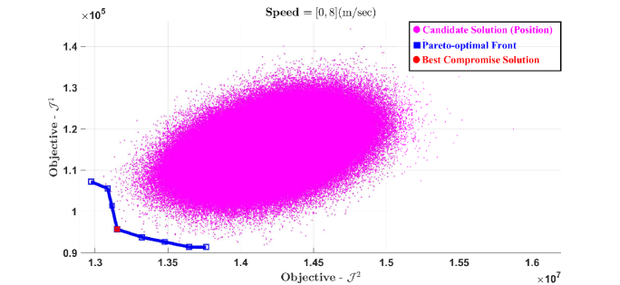
Figure 3: Objective function minimization of speed = [0, 8] (m/sec): Search history, Pareto-optimal front and best compromise solution.

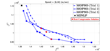
Figure 4: Objective function minimization of speed = [8, 16] (m/sec): MOPSO vs MINLP.

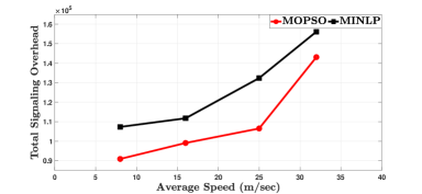
Figure 5: Average total signaling overhead: MOPSO vs MINLP.

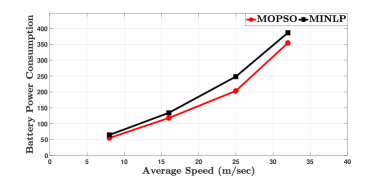
Figure 6: Average battery power consumption: MOPSO vs MINLP.

The overall quality of MOPSO convergence very close to the optimal solution is presented in terms of mean and standard deviation (STD). Table V lists the best compromise solutions of non-dominated objective functions recorded on the Pareto-optimal front considering four trials at various speed ranges. Also, Table V outlines the mean and STD of the four trials at every speed range. The accuracy of convergence can be evaluated by the percentage of STD with respect to the means, which is known as a relative standard deviation (RSD). RSD of $\boldsymbol{\mathcal{J}}^{1}$ is 0.7%, 0.7%, 1.3% and 1.26% and RSD of $\boldsymbol{\mathcal{J}}^{2}$ is 1.4%, 2.8%, 1.2% and 0.68% at the four speed ranges. Indeed, the RSD of $\boldsymbol{\mathcal{J}}^{1}$ and $\boldsymbol{\mathcal{J}}^{2}$ illustrates the remarkable performance of MOPSO when applied to the LTE networks location management. Likewise, the total power consumption has been evaluated in Table VI in terms of the mean and STD of the results obtained by MOPSO algorithm versus MINLP at different speeds. It can be noticed that MOPSO generated lower values of total power consumption than MINLP.

TABLE V: MOPSO best compromise solution of the four trials at various range of speeds

Experiment index	1	2	3	4	Mean $\pm$ STD
Speed Range	[0-8] m/sec
$\boldsymbol{\mathcal{J}}^{1}$	94343	91091	92738	93432	92901$\pm$ 1374
$\boldsymbol{\mathcal{J}}^{2}$	13342339	13325501	13436437	13204385	13327165$\pm$ 92901
Speed Range	[8-16] m/sec
$\boldsymbol{\mathcal{J}}^{1}$	97236	100491	102482	96479	99172$\pm$ 2810
$\boldsymbol{\mathcal{J}}^{2}$	14161850	14296212	14198106	14388572	14261185$\pm$ 102144
Speed Range	[16-25] m/sec
$\boldsymbol{\mathcal{J}}^{1}$	110289	107139	108643	108418	108622$\pm$ 1293
$\boldsymbol{\mathcal{J}}^{2}$	16045610	16512041	16202005	16431714	16297842$\pm$ 213392
Speed Range	[25-33] m/sec
$\boldsymbol{\mathcal{J}}^{1}$	145550	143241	144100	144786	144419$\pm$ 983
$\boldsymbol{\mathcal{J}}^{2}$	18502495	18567046	18509153	18115217	18423477$\pm$ 207541

TABLE VI: Total power consumption Mean and STD of MOPSO against MINLP at various speed ranges

Speed range	0 - 8	8 - 16	16 - 25	25 - 33
Algorithm	Mean $\pm$ STD
MOPSO	54 $\pm$ 0.82	117 $\pm$ 2.7	203 $\pm$ 3.8	354 $\pm$ 2.89
MINLP	64.5	134	248	386.5

VI Conclusion

Cellular networks are essential as they offer a variety of connectivity solutions. LTE and LTE-A provide reliable and fast wireless network service. Nonetheless, the total signaling overhead has been a concern, in particular with the rapid growth of more advanced cellular phones and phone applications. In fact, location management which allocate the idle user is directly related to the total signaling overhead. The total signaling overhead can be assessed by two elements, the total signaling cost of TAU and paging and the total inter-list handover. However, these two elements are adversely related. This study proposes a new formulation of the total signaling overhead as a true multi-objective problem where both conflicting objectives are optimized simultaneously. This novel approach is based on the multi-objective particle swarm optimization (MOPSO) which allows to minimize the total signaling overhead, and therefore bring location management in LTE networks to a qualitatively new level. The significant decrease in the total signaling overhead is achieved by minimizing the two objectives and obtaining a best compromise solution from a set of non-dominated solutions on the Pareto-optimal front. The first objective is the lessening of the total signaling cost of TAU and paging and the second objective is the minimization of the total inter-list handover. A set of experiments has been performed considering different random initialization to validate the robustness of the proposed algorithm. Location management in LTE networks using MOPSO has been examined by considering a large scale environment problem. In this problem various speed ranges have been considered with four experiments at every speed range. The best compromise solution obtained by MOPSO is compared to MINLP. Lower values of total signaling overhead and power consumption have been observed using MOPSO than MINLP. In addition, at every speed range, small values of relative standard deviation (RSD) have been observed. The robustness of MOPSO algorithm in terms of its ability to approach the optimal solution has been validated through a set of four algorithm runs performed at each level of the four different speed levels considering different random initialization conditions of the optimized parameters. Thus the proposed algorithm adequately represents a network with a variety of mobility patterns and different cells.

AUTHOR INFORMATION

Hashim A. Hashim is a Ph.D. candidate and a Teaching and Research Assistant in Robotics and Control, Department of Electrical and Computer Engineering at the University of Western Ontario, ON, Canada.
His current research interests include stochastic and deterministic filters on SO(3) and SE(3), control of multi-agent systems, control applications and optimization techniques.
Contact Information: hmoham33@uwo.ca.

Mohammad A. Abido received the B.Sc. (Honors with first class) and M.Sc. degrees in EE from Menoufia University, Shebin El-Kom, Egypt, in 1985 and 1989, respectively, and the Ph.D. degree from King Fahd University of Petroleum and Minerals (KFUPM), Dhahran, Saudi Arabia, in 1997. He is currently a Distinguished University Professor at KFUPM.
His research interests are power system control and operation and renewable energy resources integration to power systems. Dr. Abido is the recipient of KFUPM Excellence in Research Award, 2002, 2007 and 2012, KFUPM Best Project Award, 2007 and 2010, First Prize Paper Award of the Industrial Automation and Control Committee of the IEEE Industry Applications Society, 2003, Abdel-Hamid Shoman Prize for Young Arab Researchers in Engineering Sciences, 2005, Best Applied Research Award of 15thGCC-CIGRE Conference, Abu-Dhabi, UAE, 2006, and Best Poster Award, International Conference on Renewable Energies and Power Quality (ICREPQ’13), Bilbao, Spain, 2013. Dr. Abido has been awarded Almarai Prize for Scientific Innovation 2017-2018, Distinguished Scientist, Saudi Arabia, 2018 and Khalifa Award for Education 2017-2018, Higher Education, Distinguished University Professor in Scientific Research, Abu Dhabi, UAE, 2018. Dr. Abido has published two books and more than 350 papers in reputable journals and international conferences. He participated in 60+ funded projects and supervised 50+ MS and PhD students.

References

- [1] L. He, Z. Yan, and M. Atiquzzaman, “Lte/lte-a network security data collection and analysis for security measurement: A survey,” IEEE Access, vol. 6, pp. 4220–4242, 2018.
- [2] S.-I. Sou, M.-R. Li, S.-H. Wang, and M.-H. Tsai, “File distribution via proximity group communications in lte-advanced public safety networks,” Computer Networks, vol. 149, pp. 93–101, 2019.
- [3] Y.-C. Wang and C.-C. Huang, “Efficient management of interference and power by jointly configuring abs and drx in lte-a hetnets,” Computer Networks, vol. 150, pp. 15–27, 2019.
- [4] Nokia Siemens Network, “Signaling is growing 50% faster than data traffic,” 2012.
- [5] S. M. Razavi and D. Yuan, “Reducing signaling overhead by overlapping tracking area list in lte,” in Wireless and Mobile Networking Conference (WMNC), 2014 7th IFIP. IEEE, 2014, pp. 1–7.
- [6] E. Aqeeli, A. Moubayed, and A. Shami, “Dynamic son-enabled location management in lte networks,” IEEE Transactions on Mobile Computing, 2017.
- [7] P. Bonami, L. T. Biegler, A. R. Conn, G. Cornuéjols, I. E. Grossmann, C. D. Laird, J. Lee, A. Lodi, F. Margot, N. Sawaya et al., “An algorithmic framework for convex mixed integer nonlinear programs,” Discrete Optimization, vol. 5, no. 2, pp. 186–204, 2008.
- [8] M. Abido, “Multiobjective particle swarm optimization for environmental/economic dispatch problem,” Electric Power Systems Research, vol. 79, no. 7, pp. 1105–1113, 2009.
- [9] V.-S. Wong and V. C. Leung, “Location management for next-generation personal communications networks,” IEEE network, vol. 14, no. 5, pp. 18–24, 2000.
- [10] K. Munir, E. Zahoor, R. Rahim, X. Lagrange, and J.-H. Lee, “Secure and fault-tolerant distributed location management for intelligent 5g wireless networks,” IEEE Access, 2018.
- [11] D. Gu and S. Rappaport Stephen, “Mobile user registration in cellular systems with overlapping location areas,” in 1999 IEEE 49th Vehicular Technology Conference (VTC’99), vol. 1, Jul 1999, pp. 802–806 vol.1.
- [12] S.-R. Yang, Y.-C. Lin, and Y.-B. Lin, “Performance of mobile telecommunications network with overlapping location area configuration,” IEEE Transactions on Vehicular Technology, vol. 57, no. 2, pp. 1285–1292, March 2008.
- [13] K.-H. Chiang and N. Shenoy, “A 2-d random-walk mobility model for location-management studies in wireless networks,” IEEE Transactions on Vehicular Technology, vol. 53, no. 2, pp. 413–424, March 2004.
- [14] I. Widjaja, P. Bosch, and H. La Roche, “Comparison of mme signaling loads for long-term-evolution architectures,” in Vehicular Technology Conference Fall (VTC 2009-Fall), 2009 IEEE 70th. IEEE, 2009, pp. 1–5.
- [15] A. Kunz, T. Taleb, and S. Schmid, “On minimizing serving gw/mme relocations in lte,” in Proceedings of the 6th International Wireless Communications and Mobile Computing Conference. ACM, 2010, pp. 960–965.
- [16] T. Taleb, K. Samdanis, and A. Ksentini, “Supporting highly mobile users in cost-effective decentralized mobile operator networks,” IEEE Transactions on Vehicular Technology, vol. 63, no. 7, pp. 3381–3396, 2014.
- [17] S. Razavi, D. Yuan, F. Gunnarsson, and J. Moe, “Exploiting tracking area list for improving signaling overhead in LTE,” in 2010 IEEE 71st Vehicular Technology Conference (VTC’10-Spring), May 2010, pp. 1–5.
- [18] S. Razavi, D. Yuan, F. Gunnarsson, and J. Moe, “Dynamic tracking area list configuration and performance evaluation in LTE,” in 2010 IEEE GLOBECOM Workshops (GC’10 Wkshps), Dec 2010, pp. 49–53.
- [19] S. Modarres Razavi and D. Yuan, “Mitigating mobility signaling congestion in LTE by overlapping tracking area lists,” in Proceedings of the 14th ACM International Conference on Modeling, Analysis and Simulation of Wireless and Mobile Systems, ser. MSWiM ’11. New York, NY, USA: ACM, 2011, pp. 285–292.
- [20] R. C. Eberhart and J. Kennedy, “A new optimizer using particle swarm theory,” in Proceedings of the sixth international symposium on micro machine and human science, vol. 1. New York, NY, 1995, pp. 39–43.
- [21] J. Du, L. Zhao, J. Xin, J.-M. Wu, and J. Zeng, “Using joint particle swarm optimization and genetic algorithm for resource allocation in td-lte systems,” in Heterogeneous Networking for Quality, Reliability, Security and Robustness (QSHINE), 2015 11th International Conference on. IEEE, 2015, pp. 171–176.
- [22] X. Wu, S. Lei, W. Jin, J. Cho, and S. Lee, “Energy-efficient deployment of mobile sensor networks by pso,” in Asia-Pacific Web Conference. Springer, 2006, pp. 373–382.
- [23] N. A. B. Ab Aziz, A. W. Mohemmed, and M. Y. Alias, “A wireless sensor network coverage optimization algorithm based on particle swarm optimization and voronoi diagram,” in Networking, Sensing and Control, 2009. ICNSC’09. International Conference on. IEEE, 2009, pp. 602–607.
- [24] H. A. Hashim, S. El-Ferik, and M. A. Abido, “A fuzzy logic feedback filter design tuned with pso for l1 adaptive controller,” Expert Systems with Applications, vol. 42, no. 23, pp. 9077–9085, 2015.
- [25] M. A. Abido, “Optimal power flow using particle swarm optimization,” International Journal of Electrical Power & Energy Systems, vol. 24, no. 7, pp. 563–571, 2002.
- [26] M. A. Abido, “Multiobjective particle swarm optimization with nondominated local and global sets,” Natural Computing, vol. 9, no. 3, pp. 747–766, 2010.
- [27] M. Iqbal, M. Naeem, A. Anpalagan, N. N. Qadri, and M. Imran, “Multi-objective optimization in sensor networks: Optimization classification, applications and solution approaches,” Computer Networks, vol. 99, pp. 134–161, 2016.
- [28] H. A. Hashim, S. El-Ferik, B. O. Ayinde, and M. A. Abido, “Optimal tuning of fuzzy feedback filter for l1 adaptive controller using multi-objective particle swarm optimization for uncertain nonlinear mimo systems,” arXiv preprint arXiv:1710.05423, 2017.
- [29] A. E. Eltoukhy, Z. Wang, F. T. Chan, and S. Chung, “Joint optimization using a leader–follower stackelberg game for coordinated configuration of stochastic operational aircraft maintenance routing and maintenance staffing,” Computers & Industrial Engineering, vol. 125, pp. 46–68, 2018.
- [30] A. E. Eltoukhy, F. T. Chan, S. H. Chung, B. Niu, and X. Wang, “Heuristic approaches for operational aircraft maintenance routing problem with maximum flying hours and man-power availability considerations,” Industrial Management & Data Systems, vol. 117, no. 10, pp. 2142–2170, 2017.
- [31] A. E. Eltoukhy, Z. Wang, F. T. Chan, and X. Fu, “Data analytics in managing aircraft routing and maintenance staffing with price competition by a stackelberg-nash game model,” Transportation Research Part E: Logistics and Transportation Review, vol. 112, pp. 143–168, 2019.
- [32] M. Kamel, S. Elkatatny, M. Mysorewala, M. Elshafei, and A. Ai-Majed, “Online control of stick-slip in rotary steerable drilling,” in 2017 9th IEEE-GCC Conference and Exhibition (GCCCE). IEEE, 2017, pp. 1–7.
- [33] M. Kamel, M. Abido, and M. Elshafei, “Quad-rotor directional steering system controller design using gravitational search optimization,” Intelligent Automation & Soft Computing, pp. 1–11, 2017.
- [34] H. A. Hashim and M. Abido, “Fuzzy controller design using evolutionary techniques for twin rotor mimo system: a comparative study,” Computational intelligence and neuroscience, vol. 2015, no. 9, p. 11, 2015.
- [35] H. A. H. Mohamed, “Improved robust adaptive control of high-order nonlinear systems with guaranteed performance,” M. Sc, King Fahd University Of Petroleum & Minerals, vol. 1, 2014.
- [36] H. A. Hashim, B. Ayinde, and M. Abido, “Optimal placement of relay nodes in wireless sensor network using artificial bee colony algorithm,” Journal of Network and Computer Applications, vol. 64, pp. 239–248, 2016.
- [37] E. Zitzler, Evolutionary algorithms for multiobjective optimization: Methods and applications. Citeseer, 1999, vol. 63.