An Improved Accurate Solver for the Time-Dependent RTE in Underwater Optical Wireless Communications

Abstract

In this paper, an improved numerical solver to evaluate the time-dependent radiative transfer equation (RTE) for underwater optical wireless communications (UOWC) is investigated. The RTE evaluates the optical path-loss of light wave in an underwater channel in terms of the inherent optical properties related to the environments, namely the absorption and scattering coefficients as well as the phase scattering function (PSF). The proposed numerical algorithm was improved based on the ones proposed in [1, 2, 3, 4], by modifying the finite difference scheme proposed in [1] as well as an enhancement of the quadrature method proposed in [2] by involving a more accurate 7-points quadrature scheme in order to calculate the quadrature weight coefficients corresponding to the integral term of the RTE. Furthermore, the scattering angular discretization algorithm used in [3] and [4] was modified, based on which the receiver’s field of view discretization was adapted correspondingly. Interestingly, the RTE solver has been applied to three volume scattering functions, namely: the single-term HG phase function, the two-term HG phase function [5], and the Fournier-Forand phase function [6], over Harbor-I and Harbor-II water types. Based on the normalized received power evaluated through the proposed algorithm, the bit error rate performance of the UOWC system is investigated in terms of system and channel parameters. The enhanced algorithm gives a tightly close performance to its Monte Carlo counterpart improved based on the simulations provided in [7], by adjusting the numerical cumulative distribution function computation method as well as optimizing the number of scattering angles. Matlab codes for the proposed RTE solver are presented in [8].

=-15pt

I Introduction

With the prospering of the wireless communication industry over the last decades, human exploration in the underwater environment increased significantly. More recently, a notable increase in research activities in the marine medium has been witnessed, which enabled the deployment of ocean exploration and communication systems [9], [10]. By this period, several emerging underwater applications have attracted many interests, such as climate recording, ecological monitoring, oil production control, and military surveillance [11]. With this permanent emphasis on researches in the marine medium, underwater wireless sensors network concept came on for enabling the concretization of several critical commercial and military applications and services [12]. In particular, wireless communication nodes such as wireless sensors, floating buoys, and submarines, require reliable links with higher data rates in order to fulfill communication requirements and exchange a relatively huge amount of data [13].

Nowadays, underwater wireless communication systems (UWCS) are implemented using acoustic, radio-frequency (RF), or optical wireless communication. Conventional RF communication technology based on carrier-modulated signals are seriously affected by extremely severe attenuation at high frequencies due to the high concentration of salt, which is a conductive material [10], [14], e.g., the attenuation in ocean water can reach 169 dB/m for 2.4 GHz band [13]. Moreover, RF-based UWC devices demand heavy and energy-consuming antennas, making RF technology an impractical candidate for UWCS [10]. On the contrary, acoustic technology is by far the most deployed technology nowadays in the UWCS [15], as it provides a much longer transmission link range compared to its RF counterpart (i.e., up to 20 km) [16]. Nevertheless, acoustic communication is affected by some technical limitations; due to the low sound wave celerity in the water (i.e., 1500 m/s at the pure water), the acoustic link suffers from serious communication delays called latency [17]. Additionally, as the frequency range associated with acoustic communication is between tens and hundreds of Kilohertz, the available communication data rate is relatively low (e.g., in the order of Kbps). Also, similarly to their RF counterparts, acoustic transceivers are heavy, costly, and energy-consuming [10].

Optical wireless communication (OWC) is an emerging technology that received considerable attention lastly, as a promising key-enabling technology for high-speed terrestrial and underwater communications [11]. It consists of transmitting the information signals in the form of light conical beams using LED or laser devices through either the free space; i.e. visible light communication (VLC), free space optics (FSO), or the underwater medium (UOWC) [14], [18]. Due to its great potential for providing a tremendous amount of bandwidth, high security as well as immunity to interference, OWC is the most advocated solution in providing a low-latency communication link with data rates of tens of Gbps over moderate distances [19].

Generally, light propagation in the marine medium is corrupted by three main phenomena: Stochastic phenomena, namely (i) turbulence-induced fading due to sea movement as well as temperature and pressure inhomogeneities [11], (ii) pointing errors due to transceiver motion [10]. On the other hand, (iii) path-loss is a deterministic phenomenon affecting light propagation, caused mainly by photons absorption and scattering, representing the two major inherent optical properties (IOP) that quantify light power loss [20]. Absorption is the process where the photons lose their energy by conversion into another form such as chemical or heat, while scattering indicates the photons direction change due to the light interaction with the medium particles and molecules [20]. That is, the greater the scattering and absorption coefficients, the severer the power loss in the medium.

Several approaches in the literature have been proposed to analyze and predict the total light power path-loss in the marine medium. Beer-Lambert’s law is a deterministic approach, and it is the simplest model applied to evaluate the optical loss [10]. Indeed, it considers an exponential decay of the received light intensity as a function of the propagation distance, attenuation coefficient, defined as the sum of absorption and scattering coefficients, as well as source intensity. However, its main drawback lies in assuming that the scattered photons are completely lost, while in fact, some of them can still be captured at the receiver after multiple scattering, and therefore the received power is underestimated [3]. On the other hand, Monte Carlo simulation method is among popular numerical approaches to evaluate the optical path loss in underwater medium. It is a probabilistic method that emulates underwater light transmission loss by transmitting and tracking the propagation of a huge number of simulated photons [7]. Its main benefits lie in its easy implementation in computation platforms, as well as its acceptable accuracy often. However, its main limitation lies in the errors related to the random values generators as well as its long running time [10].

During the recent past years, the use of radiative transfer equation (RTE) has attracted significant attention in the fields of optics for biomedical imaging [21]. In particular, it is considered as a deterministic solution for describing light propagation in multiple absorbing and scattering medium (e.g., fluids, underwater environment), in terms of the medium IOP, such as absorption and scattering coefficients as well as the phase scattering function (PSF). Interestingly, this latter defines the scattering power distribution over the various directions in the propagation medium. In this regard, the single-term Henyey-Greenstein (STHG) function has been widely adopted as an analytical model for highly peaked forward scattering environments [3]. Nevertheless, due to the inaccurate fitting of the STHG phase function with scattering measurements for most of the realistic marine environments, the two-terms Henyey-Greenstein (TTHG) and the Fournier-Forand (FF) phase functions have been advocated as analytical models for the underwater PSF modeling.

Even though the RTE is already more than a century old, very few works along this period involved this equation for evaluating the light power loss in various scattering mediums, since it is enough complicated to solve the integro-differential RTE analytically. Actually, various numerical approaches have been used for this purpose, namely [1], [2], [3], and [4]. In [1], a numerical approach to solve the time-dependent (TD) RTE using the finite difference equation and the discrete ordinate method (DOM) was proposed. This latter consists of discretizing the angular and spatial coordinates uniformly into finite equally spaced points. Interestingly, trapeze quadrature method was used to solve the RTE integral term. The authors in [2] deployed another numerical approach for solving the steady-state time-independent (TI) RTE, based also on the DOM and the upwind finite difference scheme for the partial derivatives, as well as using the 3-points Simpson’s quadrature method to solve the integral term. In [3], an improvement was made related to the numerical proposal in [2], where an optimal non-uniform angular discretization through the Lloyd-Max algorithm [22] is proposed. Furthermore, the Gauss-Seidel iterative method was involved to solve the fully discretized system of linear equations. Finally, the proposed solver in [3] was improved in [4] by involving a two-neighbours derivative for space coordinates in addition to involving time derivative, as well as incorporating the 5-points quadrature scheme alongside with the 3-points one. It is noteworthy that the majority of the previous related works dealt with the STHG as a PSF.

In this paper, an enhancement of the numerical TD-RTE solvers developed in [3] and [4] is investigated. Distinctly to these latter where the 3 and 5-points quadrature schemes were applied to neighboring scattering angles, which is inaccurate, we involve in this paper the 7-points quadrature scheme, which we apply to infinitesimally small subintervals. Additionally, the scattering angles discretizing algorithm used in the two abovementioned works was modified. The main contributions of this paper are highlighted as follows:

• The 3 and 5-points quadrature methods used in [3] and [4], respectively, are adjusted by involving the 7-point rule given by the Newton-Cotes formula. The quadrature method aims at determining the weight coefficients in order to compute the integral term of the TD-RTE. Distinctly from [3] and [4], where the above-mentioned quadrature schemes were applied to neighboring scattering angles, which is an inaccurate approach since the step between two angles is relatively great, we propose to apply this interpolation method to the discretized infinitesimally small subintervals within the interval between two successive scattering angles.

• Distinctly from [3] and [4], the mean squared error (MSE) based algorithm, used for the scattering angles discretization, is modified. In particular, the updated version in this paper relaxes the symmetric scattering distribution considered previously. Furthermore, the receiver’s field of view (FOV) has been discretized in a similar manner to the scattering angles.

• As performed in [4], a more accurate finite upwind difference scheme, incorporating two neighbor points, is involved.

• In addition to applying the TD-RTE solver to the classical STHG function used in [3] and [4], the TTHG and FF phase functions are also adopted as PSFs in this work.

• Monte Carlo simulation provided in [7] was updated, by modifying the numerical cumulative distribution function (CDF) computation as well as optimizing the number of generated scattering angles for each subinterval of two successive distances.

• The bit error rate (BER) performance is analyzed, based on the evaluated received power, as a function of propagation time and distance as well as the system and channel parameters.

• The numerical RTE results are compared with their Monte Carlo (MC) counterparts, performed based on the proposed simulation algorithm in [7]. Furthermore, the proposed numerical RTE solver and MC simulation complexities are compared in terms of computation time.

• Matlab codes for the developed RTE Solver are presented at the end of the paper [8].

In this context, the remainder of this paper is organized as follows: Section II presents the UOWC system model as well as the improved TD-RTE solver. A numerical application of the derived results is shown in Section III. Section IV concludes the paper with some future directions.

II System Model

The light propagation on the three-dimensional space undergoes two main phenomena: (i) Absorption by which the photons energy is converted into another form, (ii) and scattering is described as the light interaction with the medium particles and molecules. As depicted in Fig. 1, the incident power $P_{I}$ , propagating toward the direction $\overrightarrow{n},$ undergoes absorption and scattering in a volume element $\Delta V$ with a width $\Delta r$, with $P_{A}$ and $P_{S}$ denote the absorbed and scattered amounts of power within $\Delta V$, respectively. A portion of the incident power, denoted $P_{T},$ will conserve the propagation direction of the incident wave. Following the energy-conservation law, one obtains

$$P_{I}=P_{A}+P_{S}+P_{T}.$$ (1)

The wavelength-dependent absorption and scattering coefficients, measured in $m^{-1},$ are defined as [10]

$$a\left(\lambda\right)=\lim_{\Delta r\rightarrow 0}\frac{P_{A}}{\Delta rP_{I}},$$ (2)

and

$$b\left(\lambda\right)=\lim_{\Delta r\rightarrow 0}\frac{P_{S}}{\Delta rP_{I}},$$ (3)

where $\lambda$ being the operating wavelength. The total attenuation coefficient $c\left(\lambda\right)$, measured in $m^{-1},$ is defined as the sum of the absorption and scattering ones as

$$c\left(\lambda\right)=a\left(\lambda\right)+b\left(\lambda\right).$$ (4)

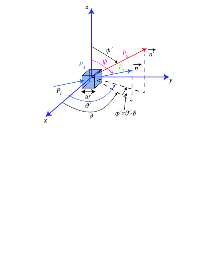
Figure 1: Light propagation in the three-dimensional space.

In the sequel, we will assume a fixed wavelength. Thus, the absorption, scattering, and attenuation coefficients are fixed.

It is known that the instantaneous light radiance is the solution of the three-dimensional TD-RTE given as [1], [20]

$$\left[\frac{1}{v}\frac{\partial}{\partial t}+\overrightarrow{n}\cdot\nabla\right]L(t,r,\vartheta,\Psi) =-cL(t,r,\vartheta,\Psi)+S\left(t\right)$$

$$+\int_{\vartheta^{\prime}=0}^{2\pi}\int_{\Psi^{\prime}=0}^{\pi}\beta\left(\vartheta,\Psi,\vartheta^{\prime},\Psi^{\prime}\right)$$

$$\times L\left(t,r,\vartheta^{\prime},\Psi^{\prime}\right)\sin\left(\Psi^{\prime}\right)d\Psi^{\prime}d\vartheta^{\prime},$$ (5)

where

• $L(t,r,\vartheta,\Psi)$ denotes the light radiance at position $r$ from the source, and at time $t$ propagating toward direction $\overrightarrow{n}$ in $W/m^{2}/sr.$ It is defined as the amount of power at distance $r$ and time $t$, per unit of surface and per unit of solid angle.

• $S\left(t\right)$ being the directed light source radiance at time $t$ in $W/m^{3}/sr.$ It is defined as the radiated power density per unit of volume per unit of solid angle.

• $\beta\left({\Psi,}\vartheta,{\Psi}^{\prime},\vartheta^{\prime}\right)$ is the volume scattering function (VSF), representing the probability density function (PDF) of the scattered power between two directions $\overrightarrow{n}$ and $\overrightarrow{n}^{\prime},$ represented by the angles $\left({\Psi,}\vartheta\right)$ and $\left({\Psi}^{\prime},\vartheta^{\prime}\right),$ respectively.

• $\nabla$ is the divergence operator.

• $v$ being the light celerity in the underwater medium.

Remark 1.

In the sequel, we will consider the 2D VSF $\beta\left(\vartheta,\vartheta^{\prime}\right)$. That is, the RTE will be solved in two dimensions rather than 3D. Consequently, the considered optical radiances are measured in $W/m^{2}/rad$. In this case, the double integral over the solid angle of a sphere, given in (5), will be replaced by a simple integral of $\vartheta^{\prime}$ argument over $\left[0,2\pi\right],$ when $\Psi^{\prime}=\frac{\pi}{2}.$ Consequently, the 2D RTE equation is expressed as

$$\left[\frac{1}{v}\frac{\partial}{\partial t}+\overrightarrow{n}\cdot\nabla\right]L(t,r,\vartheta) =-cL(t,r,\vartheta)+\int_{0}^{2\pi}\beta\left(\vartheta,\vartheta^{\prime}\right)$$

$$\times L\left(t,r,\vartheta^{\prime}\right)d\vartheta^{\prime}+S\left(t\right),$$ (6)

The VSF $\beta\left(\vartheta,\vartheta^{\prime}\right)$ is related to the PSF $\widetilde{\beta}\left(\phi^{\prime}\right)$ as [10]

$$\beta\left(\vartheta,\vartheta^{\prime}\right)=b\widetilde{\beta}\left(\phi^{\prime}\right),$$ (7)

where $\phi^{\prime}$ denotes the scattering angle between the two directions $\overrightarrow{n}$ and $\overrightarrow{n}^{\prime}$.

The scalar product of the scattering vector $\overrightarrow{n}^{\prime}$ with unit vectors $\overrightarrow{e}_{x},\overrightarrow{e}_{y}$ is given by, respectively

$$\overrightarrow{n}^{\prime}\cdot\overrightarrow{e}_{x} = \cos\vartheta^{\prime},$$ (8)

$$\overrightarrow{n}^{\prime}\cdot\overrightarrow{e}_{y} = \sin\vartheta^{\prime},$$ (9)

where $\vartheta$ and $\vartheta^{\prime}$ are defined as the angles between the $x$-axis and the propagation and scattering vectors $\overrightarrow{n}$ and $\overrightarrow{n}^{\prime}$ in the $XOY$ plane, respectively.

II-A Single Term HG Function

A popular analytical model for representing anisotropic propagation of light is the two-dimensions (2D) single term Henyey-Greenstein (STHG) scattering function given as [2]

$$\widetilde{\beta}_{STHG}\left(g,\phi^{\prime}\right)=\frac{1-g^{2}}{2\pi\left(1+g^{2}-2g\cos\phi^{\prime}\right)},0\leq g\leq 1,$$ (10)

where $g$ accounts for the scattering strength, i.e., isotropic scattering is defined for $g=0$, while as $g\$tends to $1$, a peaked scattering scenario is presented. Interestingly, it has been shown that the value $g=0.93$ represents an accurate approximation for the angular distribution of scattered light in the majority of water types [10].

II-B Two Terms HG Function

Due to the inaccurate fitting of the STHG phase function with measurements at small and large scattering angles, a linear combination of Henyey-Greenstein phase functions is sometimes used to improve the fit at small and large angles. The TTHG phase function is given as [5]

$$\widetilde{\beta}_{TTHG}\left(\alpha,g_{1},g_{2},\phi^{\prime}\right)=\alpha\widetilde{\beta}_{STHG}\left(g_{1},\phi^{\prime}\right)+(1-\alpha)\widetilde{\beta}_{STHG}\left(g_{2},\phi^{\prime}\right),$$ (11)

where $\alpha$ is a weighting factor between $0$ and $1$, $g_{1}$ and $g_{2}$ stands for scattering strength parameters. It is worth mentioning that enhanced small-angle scattering is obtained by choosing $g_{1}$ near one, and enhanced backscatter is obtained by making $g_{2}$ negative.

II-C Fournier-Forand Function

The Fournier-Forand (FF) phase function is among other PSFs that have been proposed as an alternative to the STHG and TTHG, in hydraulic optics as well as in underwater optical environments [20]. The two parameters FF phase function, introduced in [6], has a more complex analytical form compared to its STHG and TTHG counterparts. Nevertheless, it depends only on two parameters, and has higher accuracy into modeling quasi all realistic underwater phase functions. The FF PSF is expressed as [6], [23]

$$\widetilde{\beta}_{FF}\left(\mu,n_{p},\phi^{\prime}\right) =\left[\begin{array}[]{l}\left[\delta\left(1-\delta^{\upsilon}\right)-\upsilon\left(1-\delta\right)\right]\sin^{-2}\left(\frac{\phi^{\prime}}{2}\right)\\ +\upsilon\left(1-\delta\right)-\left(1-\delta^{\upsilon}\right)\end{array}\right]$$ (14)

$$\times\frac{1}{4\pi(1-\delta^{2})\delta^{\upsilon}}+\frac{1-\delta_{\pi}^{\upsilon}}{16\pi\left(\delta_{\pi}-1\right)\delta_{\pi}^{\upsilon}}$$

$$\times\left(3\cos^{2}\left(\phi^{\prime}\right)-1\right),$$ (15)

where $n_{p}$ is the real refraction index, and $\mu$ denotes is the slope parameter of the hyperbolic distribution, with $3\leq\mu\leq 5$, and

$$\upsilon = \frac{3-\mu}{2},$$ (16)

$$\delta = \frac{4}{3(n_{p}-1)^{2}}\sin^{2}\left(\frac{\phi^{\prime}}{2}\right),$$ (17)

with $\delta_{\pi\text{ }}$ being $\delta$ evaluated at $\phi^{\prime}=\pi.$

II-D Optimal Scattering Angles : Improved Algorithm

Figure 2: Non-uniform scattering directions discretization.

In [2], the authors used the uniform discrete ordinate method, based on discretizing the angular space of propagation into discrete equidistant directions. However, this approach seems accurate only for isotropic scattering environments $(g=0)$ and presents some inaccuracies for highly peaked forward scattering waters [9], [3]. Considering the TTHG and FF functions in addition to the STHG one, where the angular directions of light propagation range in the interval $\left[0,2\pi\right]$, the angular space is discretized into $K$ unequally spaced directions $\phi_{k}^{\prime},$ as shown in Fig. 2, minimizing the following mean squared error [3]

$$f(K)=\sum_{i=1}^{K}\int_{d_{i-1}}^{d_{i}}\left(\phi_{i}^{\prime}-\phi^{\prime}\right)^{2}\widetilde{\beta}_{X}\left(\Omega,\phi^{\prime}\right)d\phi^{\prime},$$ (18)

where $d_{i}$ denotes the decision thresholds, $X$ denotes either $STHG,$ $TTHG,$ or $FF$, while $\left(\Omega,\phi^{\prime}\right)$ denotes either $\left(g,\phi^{\prime}\right),$ $\left(\alpha,g_{1},g_{2},\phi^{\prime}\right),$ or $\left(\mu,n_{p},\phi^{\prime}\right),$ respectively.

In order to minimize the MSE of the above function, we must satisfy the two following conditions

$$d_{i} = \frac{\phi_{i}^{\prime}+\phi_{i+1}^{\prime}}{2};1\leq i\leq K,$$ (19)

$$\phi_{i}^{\prime} = \frac{\int_{d_{i-1}}^{d_{i}}\phi^{\prime}\widetilde{\beta}_{X}\left(\Omega,\phi^{\prime}\right)d\phi^{\prime}}{\int_{d_{i-1}}^{d_{i}}\widetilde{\beta}_{X}\left(\Omega,\phi^{\prime}\right)d\phi^{\prime}};1\leq i\leq K.$$ (20)

The non-uniform scattering angle discretization process is depicted in Algorithm 1.

Data: $K$, $g$, $\alpha$, $g_{1}$, $g_{2}$, $\mu$, $n_{p}$, $\epsilon$, PSF

Result: $\phi_{k}^{\prime}$

begin

• Initialize $\phi^{\prime}_{k}$ uniformly, i.e., $\phi_{k}^{\prime(0)}=(k-1)\frac{2\pi}{K},1\leq k\leq K$;

•  

  Setting $d_{0}=0$ ;

 

$l\leftarrow 0$;

       if PSF="STHG" then

             $\Omega\leftarrow g$;

       end if

      else if PSF="TTHG" then

             $\Omega\leftarrow\alpha,g_{1},g_{2}$;

       end if

      else

             $\Omega\leftarrow\mu,n_{p}$;

       end if

      

      repeat

•        

  Computing $d_{k}$ for $1\leq k\leq K$ using (19);

       

Calculating the new values $\phi_{k}^{\prime(l+1)}$ using (10),

(11), (15), and (20), for $1\leq k\leq K$ ;

       

$l\leftarrow l+1$;

      until $\phi_{k}^{\prime(l+1)}-\phi_{k}^{\prime(l)}<\epsilon$;

end

Algorithm 1 Optimal scattering angles.

In this paper, the Lloyd-Max algorithm, used in [3] and [4] that provides optimal angles through MSE criteria was modified. The angular discretization in the former version was symmetric with respect to the reference forward direction $\left(\phi_{1}^{\prime}=0\right),$ while in this updated one, the angular discretization is asymmetric with respect to the $x$-axis. The reference forward direction $\phi_{1}^{\prime}$ is chosen as $\phi_{1}^{\prime}\neq 0$, which is more practical as the source beam diverges through a divergent lens, by an initial divergence half-angle of $\omega.$ That is, $K$ angles will be computed in this version instead of $\frac{K}{2},$ performed in the former one.

The time coordinate is discretized uniformly into equidistant time instants $t_{n}\left(1\leq n\leq N\right)$, $\Delta t$ denotes the discretization step between two consecutive time instants $t_{n}$ and $t_{n+1}$, while $N$ accounts for the maximal number of time instants, at which the convergence of the TD-RTE solution is attained.

By discretizing (8) and (9), and plugging them as well as the time discretization into (6), one obtains

$$\eta_{k}\frac{\partial L_{k}(t_{n},r)}{\partial y}+\xi_{k}\frac{\partial L_{k}(t_{n},r)}{\partial x}+\frac{1}{v}\frac{\partial L_{k}(t_{n},r)}{\partial t} =-cL_{k}(t_{n},r)$$

$$+b\sum_{k_{s}=1}^{K}w_{k,k_{s}}L_{k_{s}}(t_{n},r)+S(t_{n}),k=1,..,K, n=1,..,N,$$ (21)

with

• $L_{k}(t_{n},r)$ being the time-dependent radiance at position $r$ propagating toward discrete direction $\phi_{k}^{\prime}$.

• $\xi_{k}=\cos\phi_{k}^{\prime},$

• $\eta_{k}=\sin\phi_{k}^{\prime}.$

• $w_{k,k_{s}}$ denotes the weight terms that substitute the integral term, with $k$ and $k_{s}$ correspond to the discrete angles of propagation and scattering directions, respectively.

It is worth mentioning that the coefficients $w_{k,k_{s}}$ in the equation above are obtained through quadrature method, detailed in the next subsection.

II-E Accurate Computation of the Integral Term

In this subsection, in order to solve numerically the integral on the right-hand side of (6), we incorporate the Simpson’s method alongside with the 5-points and 7-points Boole’s rule given by the Newton-Cotes formulas [24, Eqs. (25.4.14), (25.4.18)], in order to calculate the weight terms $w_{k,k_{s}}$ given as

$$w_{1,k_{s}}=\sum\limits_{l=1}^{M}S_{k_{s}}(l);1\leq k_{s}\leq K,$$ (22)

where $S_{k_{s}}(l)$ is defined in (20) at the top of the next page, $h_{k_{s}}=\frac{\Delta\phi_{k_{s}}^{\prime}}{M}$ denotes an infinitesimally small quadrature discretization step, $\Delta\phi_{k_{s}}^{\prime}$ is the difference between the angles $\phi_{k_{s}}^{\prime}$ and $\phi_{k_{s}+1}^{\prime},$ and $M$ is the number of discrete points within this area, assumed to be the same for all sub-intervals of scattering angles. $\widetilde{\beta}_{X}\left(\Omega,\phi^{\prime}\right)$ is the PDF of the scattered photons, its integration over $2\pi$ equals $1.$ Then, it follows from the equation above that all the terms $w_{1,k_{s}}$ should be normalized by $\sum\limits_{k_{s}=1}^{K}w_{1,k_{s}}.$ The remaining terms $w_{k,k_{s}}$ can be calculated using the formula [3]

$$S_{k_{s}}(l)=\begin{cases}\frac{h_{k_{s}}}{18}\left(\widetilde{\beta}_{X}\left(\Omega,\phi_{k_{s}}^{\prime}\right)+2\widetilde{\beta}_{X}\left(\Omega,\phi_{k_{s}}^{\prime}+h_{k_{s}}\right)\right),l=1,\\ \frac{2h_{k_{s}}}{36}\left(\widetilde{\beta}_{X}\left(\Omega,\phi_{k_{s}}^{\prime}\right)+4\widetilde{\beta}_{X}\left(\Omega,\phi_{k_{s}}^{\prime}+h_{k_{s}}\right)+\widetilde{\beta}_{X}\left(\Omega,\phi_{k_{s}}^{\prime}+2h_{k_{s}}\right)\right),l=2\\ \frac{4h_{k_{s}}}{180}\left(\begin{array}[]{l}7\widetilde{\beta}_{X}\left(\Omega,\phi_{k_{s}}^{\prime}\right)+32\widetilde{\beta}_{X}\left(\Omega,\phi_{k_{s}}^{\prime}+h_{k_{s}}\right)+12\widetilde{\beta}_{X}\left(\Omega,\phi_{k_{s}}^{\prime}+2h_{k_{s}}\right)\\ +32\widetilde{\beta}_{X}\left(\Omega,\phi_{k_{s}}^{\prime}+3h_{k_{s}}\right)+7\widetilde{\beta}_{X}\left(\Omega,\phi_{k_{s}}^{\prime}+4h_{k_{s}}\right)\end{array}\right),l=3\\ \frac{6h_{k_{s}}}{5040}\left(\begin{array}[]{l}41\widetilde{\beta}_{X}\left(\Omega,\phi_{k_{s}}^{\prime}+(l-4)h_{k_{s}}\right)+216\widetilde{\beta}_{X}\left(\Omega,\phi_{k_{s}}^{\prime}+(l-3)h_{k_{s}}\right)+27\widetilde{\beta}_{X}\left(\Omega,\phi_{k_{s}}^{\prime}+(l-2)h_{k_{s}}\right)\\ +272\widetilde{\beta}_{X}\left(\Omega,\phi_{k_{s}}^{\prime}+(l-1)h_{k_{s}}\right)+27\widetilde{\beta}_{X}\left(\Omega,\phi_{k_{s}}^{\prime}+lh_{k_{s}}\right)+216\widetilde{\beta}_{X}\left(\Omega,\phi_{k_{s}}^{\prime}+(l+1)h_{k_{s}}\right)\\ +41\widetilde{\beta}_{X}\left(\Omega,\phi_{k_{s}}^{\prime}+(l+2)h_{k_{s}}\right)\end{array}\right);4\leq l\leq M-3\\ \frac{4h_{k_{s}}}{180}\left(\begin{array}[]{l}7\widetilde{\beta}\left(\Omega,\phi_{k_{s}+1}^{\prime}-4h_{k_{s}}\right)+32\widetilde{\beta}\left(\Omega,\phi_{k_{s}+1}^{\prime}-3h_{k_{s}}\right)+12\widetilde{\beta}\left(\Omega,\phi_{k_{s}+1}^{\prime}-2h_{k_{s}}\right)\\ +32\widetilde{\beta}\left(\Omega,\phi_{k_{s}+1}^{\prime}-h_{k_{s}}\right)+7\widetilde{\beta}\left(\Omega,\phi_{k_{s}+1}^{\prime}\right)\end{array}\right),l=M-2\\ \frac{2h_{k_{s}}}{36}\left(\widetilde{\beta}_{X}\left(\Omega,\phi_{k_{s}+1}^{\prime}-2h_{k_{s}}\right)+4\widetilde{\beta}_{X}\left(\Omega,\phi_{k_{s}+1}^{\prime}-h_{k_{s}}\right)+\widetilde{\beta}_{X}\left(\Omega,\phi_{k_{s}+1}^{\prime}\right)\right),l=M-1\\ \frac{h_{k_{s}}}{18}\left(\widetilde{\beta}_{X}\left(\Omega,\phi_{k_{s}+1}^{\prime}-h_{k_{s}}\right)+2\widetilde{\beta}_{X}\left(\Omega,\phi_{k_{s}+1}^{\prime}\right)\right),l=M.\end{cases}$$ (20)

$$w_{k,k_{s}}=w_{1,|k-k_{s}|+1},$$ (21)

Figure 3: Areas rates for the adopted quadrature scheme, using the computation on 2, 3, 5, and 7 points calculated at terms $S_{k_{s}}(l);l=1,...,M$.

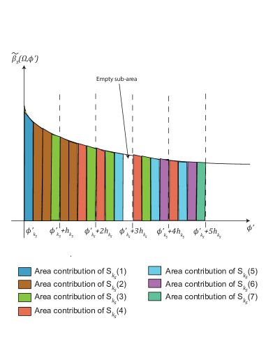
Figure 4: Areas rates for the 5-points quadrature scheme used in [4], using the computation on 2, 3, and 5 points calculated at terms $S_{k_{s}}(l);l=1,...,M$.

One can remark clearly from (20) that the quadrature terms involving 5 points (i.e., $S_{k_{s}}(3)$ and $S_{k_{s}}(M-2))$ were scaled by $1/2$ from the original equation [24, Eq. (25.4.14)], while the remaining terms involving two, five and seven points were scaled by a factor of $1/6$ from [24, Eqs. (25.4.1)-(25.4.16)]. In fact, the area delimited by the function’s curve and the $\phi^{\prime}-$axis was divided in successive areas. Indeed, as represented in Fig. 3, the area $\mathcal{A}_{l}$ delimited by the interval $\left[\phi_{k_{s}}^{\prime}+lh_{k_{s}},\phi_{k_{s}}^{\prime}+(l+1)h_{k_{s}}\right],$ $5\leq$ $l\leq M-6$ will be recomputed  in the case of 7-points’ interpolation by three terms on the left, i.e., $S_{k_{s}}(l-1)$, $S_{k_{s}}(l)$ and $S_{k_{s}}(l+1)$ as well as by three terms on the right namely, $S_{k_{s}}(l+2),$ $S_{k_{s}}(l+3)$, and $S_{k_{s}}(l+4).$ Therefore, each of these terms is scaled by the same factor $1/6$ to get the exact area rate. Explicitly, we have

$$\mathcal{A}_{l}\mathcal{=}\sum\limits_{i=0}^{5}S_{k_{s}}\left(l-1+i\right),5\leq l\leq M-6.$$ (22)

Besides, it can be noticed that the areas $\left[\phi_{k_{s}}^{\prime},\phi_{k_{s}}^{\prime}+h_{k_{s}}\right]$ and $\left[\phi_{k_{s}}^{\prime}+h_{k_{s}},\phi_{k_{s}}^{\prime}+2h_{k_{s}}\right]$ are filled through the terms $\left(S_{k_{s}}(1),S_{k_{s}}(2),S_{k_{s}}(3),S_{k_{s}}(4)\right)$ and $\left(S_{k_{s}}(2),S_{k_{s}}(3),S_{k_{s}}(4)\right.$, $\left.S_{k_{s}}(5)\right)$, with scale factors $\left(\frac{1}{6},\frac{1}{6},\frac{1}{2},\frac{1}{6}\right)$ and $\left(\frac{1}{6},\frac{1}{2},\frac{1}{6},\frac{1}{6}\right)$, respectively. Nevertheless, there is an overfill by $\frac{1}{6}$ of the area associated to the interval $\left[\phi_{k_{s}}^{\prime}+lh_{k_{s}},\phi_{k_{s}}^{\prime}+(l+1)h_{k_{s}}\right],$for $l=3,M-5,$ as indicated in the rectangle labeled "overfill" within the interval $\left[\phi_{k_{s}}^{\prime}+3h_{k_{s}},\phi_{k_{s}}^{\prime}+4h_{k_{s}}\right]$ in Fig. 3, as well as $\frac{1}{6}$ of the area $\left[\phi_{k_{s}}^{\prime}+lh_{k_{s}},\phi_{k_{s}}^{\prime}+(l+1)h_{k_{s}}\right],$ for $l=4,M-6,$ not filled as represented by the blank bar within the interval $\left[\phi_{k_{s}}^{\prime}+4h_{k_{s}},\phi_{k_{s}}^{\prime}+5h_{k_{s}}\right]$ in the same figure, within the whole area $\left[\phi_{k_{s}}^{\prime},\phi_{k_{s}+1}^{\prime}\right].$ Interestingly, the 5-points scheme developed in [4] and presented in Fig. 4 is based on computing the areas $\left[\phi_{k_{s}}^{\prime}+lh_{k_{s}},\phi_{k_{s}}^{\prime}+(l+1)h_{k_{s}}\right]$ $(l=1,..,M-2)$ using the 2, 3, and 5-points computation, with corresponding scales of $\frac{1}{4},$ $\frac{1}{2},$ and $\frac{1}{4}$, respectively, so as to fill the whole area delimited by the $\phi^{{}^{\prime}}$ axis and the function’s curve.

Remark 2.

It is worthy to mention that this quadrature scheme was applied up only to 5-points quadrature scheme equivalently in [4] as depicted in Fig. 4, by considering $\left[\phi_{1}^{\prime},\phi_{K}^{\prime}\right]$ as the surface of interest, and the points $\phi_{k_{s}}^{\prime}(1\leq k_{s}\leq K)$ as the integration points. However, this quadrature method is inaccurate considering this scheme, since the non-uniform discretization step $\Delta\phi_{k_{s}}^{\prime}$ of each interval is relatively great (e.g., $\Delta\phi_{1}^{\prime}=6{{}^{\circ}})$, and consequently, that applied method is not valid.

II-F Finite Difference Equation

As a third step of the process, and in order to solve the spatial derivative terms in (21), the upwind finite difference equation is involved.

The area between the transmitter and the receiver is divided into $I$ grid points horizontally and $J$ grid points vertically. It is noteworthy that in order to improve the computation accuracy of the upwind finite difference scheme used in [1], we involve one more point in each formula.

The Taylor-series development of the radiance function $L_{i,j,k}(t_{n})$ near the four neighbor points $(i\pm 1,j),(i\pm 2,j)$ close to $(i,j),$ with $i=1,...,I$ and $j=1,...,J,$ is given by

$$L_{i\pm 1,j,k}(t_{n}) \approx L_{i,j,k}(t_{n})\pm\Delta y\frac{\partial L_{i,j,k}(t_{n})}{\partial y},$$ (23)

$$L_{i\pm 2,j,k}(t_{n}) \approx L_{i,j,k}(t_{n})\pm 2\Delta y\frac{\partial L_{i,j,k}(t_{n})}{\partial y}.$$ (24)

In a similar manner, the same development is performed at the points $(i,j\pm 1),(i,j\pm 2).\qquad\qquad$

By performing some algebraic manipulation on the equations above, and using the same reasoning likewise for the other cases of $\xi_{k},\eta_{k}$, improved finite difference formulas are obtained as

$$\frac{\partial L_{i,j,k}(t_{n})}{\partial y}\approx\left\{\begin{array}[]{c}\frac{2L_{i,j,k}(t_{n})-L_{i-1,j,k}(t_{n})-L_{i-2,j,k}(t_{n})}{3\Delta y},\eta_{k}>0\\ \frac{L_{i+1,j,k}(t_{n})+L_{i+2,j,k}(t_{n})-2L_{i,j,k}(t_{n})}{3\Delta y},\eta_{k}<0\end{array}\right.$$ (25)

$$\frac{\partial L_{i,j,k}(t_{n})}{\partial x}\approx\left\{\begin{array}[]{c}\frac{2L_{i,j,k}(t_{n})-L_{i,j-1,k}(t_{n})-L_{i,j-2,k}(t_{n})}{3\Delta x},\xi_{k}>0\\ \frac{L_{i,j+1,k}(t_{n})+L_{i,j+2,k}(t_{n})-2L_{i,j,k}(t_{n})}{3\Delta x},\xi_{k}<0\end{array}\right.,$$ (26)

where $\Delta x$ and $\Delta y$ stand for the discretization steps in the $x$ and $y$ axes, respectively.

One can ascertain that each partial derivative is associated to two formulas depending on the sign of $\xi_{k}$ and $\eta_{k}.$

Regarding the time derivative, the forward Euler difference formula was used as[1]

$$\frac{\partial L_{i,j,k}(t_{n})}{\partial t}=\frac{L_{i,j,k}(t_{n+1})-L_{i,j,k}(t_{n})}{\Delta t};n=1,..,N-1,$$ (27)

with $\Delta t$ being the discretization step for the time coordinate.

By plugging the partial derivatives (25), (26), and (27) into (21), and performing some manipulations, we obtain the recursive equation (28) given at the top of the next page.

$$L_{i,j,k}(t_{n+1}) =L_{i,j,k}(t_{n})\left[1-cv\Delta t\pm\frac{2\eta_{k}v\Delta t}{3\Delta y}\pm\frac{2\xi_{k}v\Delta t}{3\Delta x}\right]\mp\eta_{k}v\Delta t\frac{L_{i\pm 1,j,k}(t_{n})+L_{i\pm 2,j,k}(t_{n})}{3\Delta y}$$

$$\mp\xi_{k}v\Delta t\frac{L_{i,j\pm 1,k}(t_{n})+L_{i,j\pm 2,k}(t_{n})}{3\Delta x}+bv\Delta t\sum_{k_{s}=1}^{K}w_{k,k_{s}}L_{i,j,k_{s}}(t_{n})+v\Delta tS_{0}.$$ (28)

It is noteworthy that the above equation depicts the recursive numerical solution of the proposed TD-RTE solver for the instantaneous light radiance, in terms of the system and channel parameters, namely the source radiance, the discretization steps in space and time coordinates, the number of directions, scattering and absorption coefficient, and light celerity in the medium as well.

Figure 5: Collimated beam divergence through a divergent lens.

Without loss of generality, we consider a point source with constant power over time $S_{0},$ defined at a specific point in the transmitter plane, $\left(\text{i.e., }1,\frac{I-1}{2}+1\right)$. In practice, the total transmit power is radiated in the form of a collimated beam, through a divergent optical lens with a certain focal length $f^{\prime}$ with an associated divergence half-angle $\omega,$ so as to produce a divergent beam [7]. $f^{\prime}$ and $\omega$ are related as

$$f^{\prime}=-\frac{x_{0}}{\omega},$$ (29)

with $x_{0}$ being the beam waist radius at the lens as shown in Fig. 5. In this case, the source radiance equals to the ratio between the source power and a circular surface of radius $x_{0}$ and to the divergence angle $2\omega$.

Remark 3.

It is worthy to mention that by neglecting the radiance variations over time $\left(i.e.,\frac{\partial L_{i,j,k}(t)}{\partial t}=0\right),$ the light radiance $L_{i,j,k}(t_{n})$ becomes time-independent. That is, the TD-RTE equation in (28) becomes TI-RTE expressed as

$$L_{i,j,k}^{(l+1)} =\left(\frac{1}{\mp\frac{2\eta_{k}}{3\Delta y}\mp\frac{2\xi_{k}}{3\Delta x}+c}\right)\left(\mp\eta_{k}\frac{L_{i\pm 1,j,k}^{(l)}+L_{i\pm 2,j,k}^{(l)}}{3\Delta y}\right.$$

$$\left.\mp\xi_{k}\frac{L_{i,j\pm 1,k}^{(l)}+L_{i,j\pm 2,k}^{(l)}}{3\Delta x}+b\sum_{k_{s}=1}^{K}w_{k,k_{s}}L_{i,j,k_{s}}^{(l)}+S_{0}\right),$$ (30)

where $l$ denotes the solution iteration index.

II-G Received Power Calculation

In our analysis, the receiver is placed on the $YOZ$ plane. Knowing that the calculated radiance is performed in the $XOY$ plane, the received power is calculated by summing up the light radiance at grid points in the receiver plane perpendicular to the $x-$axis (i.e., $YOZ$ plane). Without loss of generality, we assume that the receiver aperture placed at the receiver plane is divided into $\frac{\Delta y}{2}-$equidistant circular surfaces, being defined as [3]

$$A_{l}=\left\{\begin{array}[]{l}\pi\left(\frac{\Delta y}{2}\right)^{2},l=1\\ 2\pi\left(\Delta y\right)^{2}\left(l-1\right),2\leq l\leq L\end{array}\right.,$$ (31)

where $L$ denotes the number of the circular surfaces within the receiver aperture given in terms of the receiver aperture of radius $R$

$$L=\frac{R}{\Delta y}.$$ (32)

Let $\Delta\phi_{p}^{\prime}$, with $1\leq p\leq P,$ denotes the difference between two directions $\phi_{p}^{\prime}$ and $\phi_{p+1}^{\prime}$ within the receiver FOV in the $XOY$ plane, discretized in the same way as the scattering angles following equation (19) and (20), with $P$ denotes the total number of discrete directions within the receiver FOV. Without loss of generality, the radiance within the angle interval delimited by $\Delta\phi_{p}^{\prime}$ in $XOY\$plane, is assumed to be constant. By considering also symmetric scattering in the elevation direction, the surface power density is uniform within each elementary circular surface within the receiver aperture. Therefore, the total received power can be expressed as [3]

$$P_{r}(t_{n})=\sum_{l=1}^{L}A_{l}\sum_{p=1}^{P}\Delta\phi_{p}^{\prime}L_{l+\left(\frac{I-1}{2}\right),J,p}(t_{n}),n=1,...,N,$$ (33)

Data: $K$, $g$, $\alpha$, $g_{1}$, $g_{2}$, $\mu$, $n_{p}$, $\epsilon$, PSF, $\Delta x$, $\Delta y$, $\Delta t$, $t_{N}$, $x_{max}$, $y_{max}$, $R$, $S_{0}$, $FOV$, $P$

Result: $L_{i,j,k}(t_{n})$,$P_{r}(t_{n})$

begin

•  

  Discretize $\phi^{\prime}_{k}$ with non-uniform distribution

      $\phi^{\prime}_{k}$= Optimal scattering angles $\left(K,g,\alpha,g_{1},g_{2},\mu,n_{p},\epsilon,PSF\right)$,

$1\leq k\leq K$;

 

Computing the quadrature terms $w_{k,k_{s}}$

for $k,k_{s}\in[1,K]$ using (20) and (21);

$I\leftarrow\lfloor\frac{y_{max}}{\Delta y}\rfloor+1$; • $J\leftarrow\lfloor\frac{x_{max}}{\Delta x}\rfloor+1$; • $\phi^{\prime}_{p}\leftarrow\phi^{\prime}_{k}$ for $\phi^{\prime}_{k}\in FOV,k=1,..,K,p=1,..,P$; • $L\leftarrow\frac{R}{\Delta y}$; • $N\leftarrow\lfloor\frac{t_{N}}{\Delta_{t}}\rfloor+1$; •   Calculate iteratively the radiance $L_{i,j,k}(t_{n})$

      using (28) for $i=1,..,I$, $j=1,..,J$, $k=1,..,K$,

and $n=1,..,N$;

 

Evaluate the total received power $P_{r}(t_{n})$,

      using (33) ;

end

Algorithm 2 RTE power computation.

It is worthy to mention that the Matlab code of Algorithm 2 for the RTE resolution and power computation is presented in Appendix A, as well as in [8].

III BER performance of UOWC

In this section, and based on the derived results, we investigate the bit error rate (BER) performance of the underwater optical wireless communication system subject to absorption and scattering, in terms of channel and system parameters.

III-A Signal-to-Noise Ratio

The instantaneous signal-to-noise ratio (SNR) at the output of a receiver employing the direct detection technique, in the presence of thermal and shot noise, is expressed as [4], [18], [25]

$$SNR\left(t_{n}\right) =\frac{I_{P}^{2}(t_{n})}{N_{0}}=\frac{\left(R_{s}FP_{r}\left(t_{n}\right)\right)^{2}}{\sigma_{s}^{2}+\sigma_{th}^{2}},$$ (34)

$$=\frac{\left(R_{s}FP_{r}\left(t_{n}\right)\right)^{2}}{2q(I_{P}(t_{n})+I_{D})B_{w}+\frac{4\kappa T_{e}B_{w}}{R_{L}}},$$

where

• $I_{P}(t_{n}):$ Incident light photo current $(A),$

• $N_{0}:$ Total noise power ($W),$

• $R_{s}:$ Photodetector responsivity ($A/W)$,

• $F:$ Photodetector gain factor ($F=1$ for PIN photodetector),

• $\sigma_{s}^{2}:$ Shot noise power ($W),$

• $\sigma_{th}^{2}:$ Thermal noise power ($W),$

• $q:$ Electrical elementary charge ($1.6\times 10^{-19}C$),

• $I_{D}:$ Shot noise dark current $(A),$

• $B_{w}:$ Electrical filter bandwidth $(Hz)$,

• $\kappa:$ Boltzmann constant $(J\cdot K^{-1}),$

• $T_{e}:$ Receiver temperature ($K$),

• $R_{L}:$ Electrical receiver load resistance ($\Omega).$

III-B Bit Error Rate

The BER of a communication system employing On-Off Keying (OOK) modulation scheme, with respect to a received SNR is defined as [18, Eq. (4.24)]

$$P_{e}\left(t_{n}\right) =Q\left(\sqrt{SNR(t_{n})}\right)$$

$$=Q\left(\frac{R_{s}FP_{r}\left(t_{n}\right)}{\sqrt{2q(I_{P}(t_{n})+I_{D})B_{w}+\frac{4\kappa T_{e}B_{w}}{R_{L}}}}\right),$$ (35)

with $Q\left(.\right)$ denotes the Gaussian $Q$-function [26, Eq. (4.1)]. Note that the values of $R_{s},$ $F,$ and $I_{D}$ can be usually retrieved from the datasheet of the photodiode product.

IV Performance and Complexity evaluations

This section presents the evaluation performance of the proposed TD-RTE solver in terms of computation accuracy as well as complexity. The TD-RTE results are given in three dimensions (3D) as a function of the propagation distance as well as time instants, while the TI-RTE results are shown in two dimensions (2D) versus the distance. The respective MATLAB codes of the proposed RTE solver are available in [8]. The RTE and MC simulations complexities are depicted in terms of time consumption per each computation step. We depict a single scattering scenario per each PSF among the three considered scattering functions, for fixed values of $g=0.93$ for the STHG function, $\alpha=0.9832,g_{1}=0.8838,g_{2}=-0.9835$ for the TTHG function, while we set $n=1.33,$ $\mu=$ $3.483$ for the Fournier-Forand scattering model. Two water types are taken into account, namely Harbor-I ($b=0.91,$ $c=1.1)$ and Harbor-II ($b=1.8177,$ and $c=2.2)$ waters with: $Y=20$ cm as the tank altitude, $t_{N}=20$ ns, $\Delta x=5$ cm, $\Delta y=1$ cm, and $\Delta t=25$ ps as the discretization steps in the $x$-axis, $y$-axis, and time coordinate, respectively, and $K=22$ as the number of discrete directions. Additionally, we considered a transmitting optical lens with a beam waist radius of $x_{0}=1$ mm. The values of $R_{s}$, $I_{D}$, and $T_{e}$ were taken from [25]. The respective Monte Carlo results were performed based on the simulations provided in [7]. In this regard, the CDF numerical computation in this latter was modified in order to evaluate the CDF with respect to the generated scattering angles accurately. Furthermore, the number of generated angles was adjusted as a function of the propagation distance.

Figs. 6-10 depict the TI-RTE normalized received power results over time versus the distance over Harbor-I and Harbor-II water types, assuming STHG scattering function. Actually, determining the number of discrete points $M$ within each interval $[\phi_{k_{s}}^{\prime},\phi_{k_{s}+1}^{\prime}]$ is of paramount importance to improve the accuracy of the proposed RTE solver. Particularly, we depict in Figs. 6-8 the RTE solver behavior using the considered quadrature schemes, namely 3-points, 5-points, and 7-points schemes. One can remark clearly that the curves corresponding to 3-points and 5-points schemes shown in Fig. 6, Fig. 7, and Fig. 10 converge to the exact solution by increasing the number of discretization points $M$ (lower discretizing step $h_{k_{s}}$) within each surface $[\phi_{k_{s}}^{\prime},\phi_{k_{s}+1}^{\prime}]$ $($i.e., $M=50$ for 3-points, and $M=40$ for 5-points), while for the 7-points scheme in figures 8 and 10, the convergence needs a lesser number of points than for the 3-points and 5-points schemes (i.e., $M=7$).

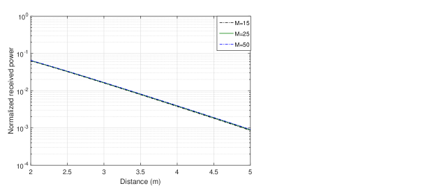
Figure 6: Average normalized received power over time propagation distance in a Harbor-II turbid water medium for the STHG function using 3-pts scheme.

Figure 7: Average normalized received power over time propagation distance in a Harbor-II turbid water medium for the STHG function using 5-pts scheme.

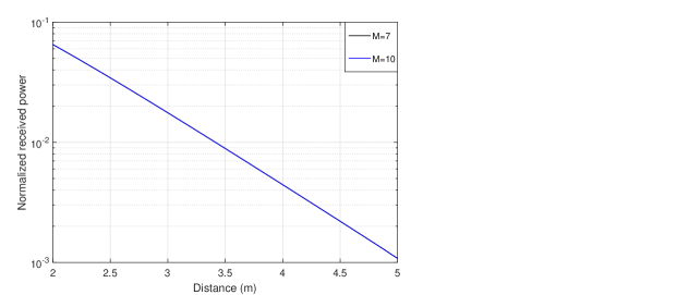
Figure 8: Average normalized received power over time propagation distance in a Harbor-II turbid water medium for the STHG function using 7-pts scheme.

Figure 9: Normalized received power versus propagation distance in a Harbor-II turbid water medium for the STHG function.

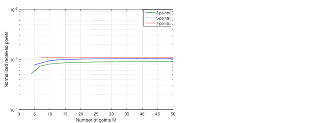
Figure 10: Normalized received power versus propagation distance in a Harbor-II turbid water medium for the STHG function.

In terms of computation complexity of the adopted quadrature schemes, Table I shows the evaluation time in seconds of the implemented 7-points quadrature scheme, for various values of the scattering angles number $K$, compared with the 3 and 5-points schemes developed in [3] and [4], respectively. These latter were adapted similarly as performed to the 7-points scheme, where they were applied for infinitesimally small sub-intervals between two successive scattering angles. Additionally, the respective number of points $M$ within each subinterval of two successive scattering angles is taken as $M=7,$ $40,$ and $50$ for the 3, 5, and 7-points schemes, respectively. Interestingly, it can be noticed that the 7-points schemes is $8$-$20$ ms less than its 3 and 5 counterparts. In fact, the higher the number of points $M$, the greater the computation time needed. Furthermore, one can ascertain that the time consumption increases slightly as a function of $K$ for the aforementioned schemes. Additionally, it can be obviously seen that the total consumed time slightly differs between the 3 schemes. In fact, since the quadrature weight coefficients are calculated once and outside the main loops $(i.e.,$ $i=1,...,I;$ $j=1...,J;$ $k=1,...,K;$ $n=1,...,N),$ the computation time is not impacted significantly.

TABLE I: Evaluation time of the numerical integration quadrature schemes (in seconds).

	3 points	5 points	7 points
$22$	0.0139	0.0132	0.0017
$26$	0.0147	0.0134	0.0027
$30$	0.0187	0.0148	0.0052
$35$	0.0175	0.0142	0.0063
$40$	0.0229	0.0151	0.0070
$50$	0.0276	0.0165	0.0078

Figs. 11-13 depict the TD-RTE normalized received power result versus distance and time, for Harbor-I, in three dimensions, taking into account the considered scattering functions (STHG, TTHG, and FF). One can ascertain that the received power decreases as a function of the distance, i.e., the farther the communication nodes are, the higher the power path-loss is due to water attenuation phenomena. Moreover, we ascertain that at initial time instants, the received power at a given distance is lower initially, and starts gradually increasing as a function of time until reaching the convergence level when the received power remains constant in time. Actually, at initial time instants, few photons reach the receiver plane, and consequently, it results in lower received power. More photons reach the receiver side resulting in an increase of the received power versus time.

Figure 11: Normalized received power in 3D versus distance and time, considering STHG function and a receiver aperture of 10cm.

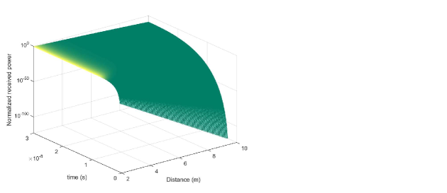
Figure 12: Normalized received power in 3D versus distance and time, considering TTHG function and a receiver aperture of 10cm.

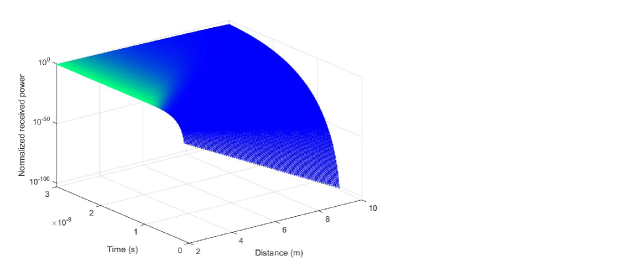
Figure 13: Normalized received power in 3D versus distance and time, considering FF function and a receiver aperture of 10cm.

Figs. 14-16 depict the TI-RTE normalized received power results in two dimensions computed by RTE numerical solver as well as the respective Monte Carlo results by considering the adopted volume scattering functions (i.e., STHG, TTHG, and FF). The numerical time-independent RTE results correspond to the average normalized received power over time. We can notice obviously that the power loss in Harbor-I water type is greater compared to the Harbor-II case. That is, the higher the scattering coefficient is (i.e., $b=0.91$ for Harbor-I and $b=1.8177$ for Harbor-II), the greater is the path-loss, and consequently, the system performance degrades. Additionally, for Fig. 14, one can note clearly the matching between the proposed numerical scaled RTE curves as well as MC results considering STHG function, on the various propagation distances values, while the RTE solver proposed in [3] yields a significant gap with MC curves, which proves the computation accuracy of the proposed numerical solver. A similar behavior can be noticed in Fig. 15 and Fig. 16 for the TTHG and FF scattering functions, and more particularly for the Harbor-I water type, while a slight gap is noticed between the proposed RTE solver and MC simulation curves at higher distances for the Harbor-II case.

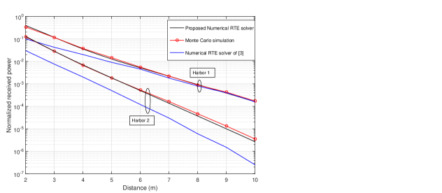
Figure 14: Average normalized received power over time versus distance considering STHG function and a receiver aperture 10cm.

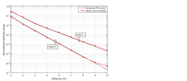
Figure 15: Average normalized received power over time versus distance considering TTHG function and a receiver aperture 10cm.

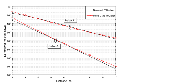
Figure 16: Average normalized received power over time versus distance considering FF function and a receiver aperture 10cm.

Fig. 17 depicts the total time consumption comparison between the proposed numerical RTE solver and Monte Carlo simulation. One can notice clearly the logarithmic increase of the MC scheme time consumption in the log-scale, which corresponds to a linear increase in the linear scale. On the other hand, we remark also that the computation time of the proposed RTE solver as well as the one proposed in [3] remains constant. In addition to this, we can notice that the respective complexities of the proposed RTE solver and the one in [3] are very close, in terms of computation complexity. Importantly, the main outcome of this result is the difference in complexity between the proposed numerical RTE solver and its MC counterpart. That is, the numerical RTE solver can achieve accurate results, with a remarkably reduced complexity compared to MC method.

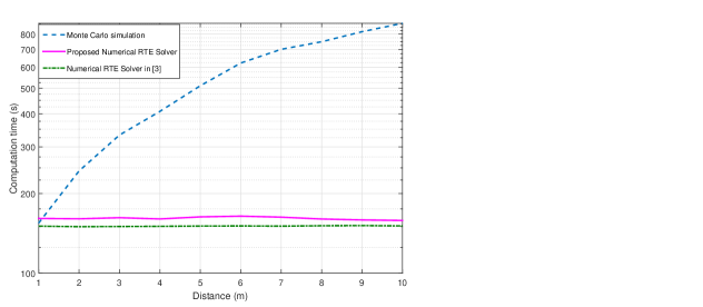
Figure 17: Computation time consumption comparison between Numerical RTE Solver and Monte Carlo simulation.

Figs. 18-23 depicts the BER performance of the communication system in 2D and 3D, based on (35) for both water types, for the considered VSF functions. The 2D curves correspond to the average normalized received power over time. In a similar manner to the power behavior, one can remark obviously that the BER increases as a function of the propagation distance. That is, the greater the propagation distance is, the more important is the path-loss, and consequently, the BER performance degrades. Additionally, the BER decreases with the increase of the received power as a function of the time. Also, Harbor-I water type exhibits a lower bit error rate to Harbor-II one.

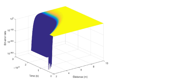
Figure 18: Bit error rate performance of the considered system in 3D, based on time-dependent RTE resolution considering STHG function (aperture: 10cm).

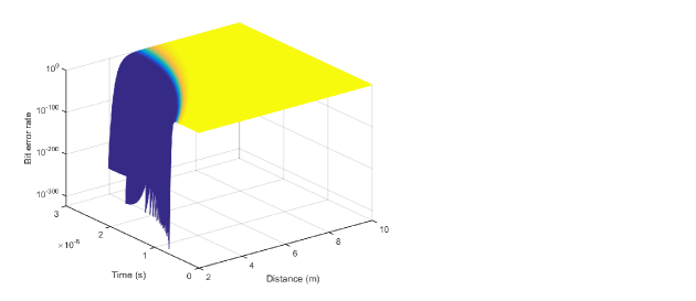
Figure 19: Bit error rate performance of the considered system in 3D, based on time-dependent RTE resolution considering TTHG function (aperture: 10cm).

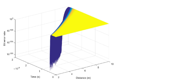
Figure 20: Bit error rate performance of the considered system in 3D, based on time-dependent RTE resolution considering FF function (aperture: 10cm).

Figure 21: Bit error rate performance of the considered system based on the average received power over time, considering STHG function (aperture: 10cm).

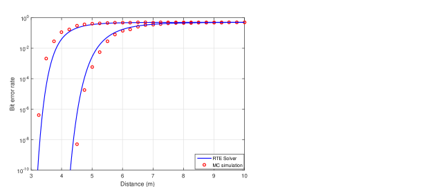
Figure 22: Bit error rate performance of the considered system based on the average received power over time, considering TTHG function (aperture: 10cm).

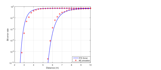
Figure 23: Bit error rate performance of the considered system based on the average received power over time, considering FF function (aperture: 10cm).

V Conclusion

In this paper, an improved time-dependent RTE numerical evaluation algorithm is proposed, in order to solve the radiative transfer equation that quantifies the light propagation loss in the underwater medium. The proposed RTE solver was applied for three types of volume scattering functions namely, the STHG, TTHG, and FF PSFs. Boole’s rule given by the 5-points and 7-points Newton-Cotes formula was incorporated as a quadrature method alongside with the two and three points Simpson’s method in order to solve the integral term. The upwind finite difference scheme was also improved by adding one more neighbor point. Furthermore, the MSE-based algorithm for scattering angles discretization was modified from [3], [4]. The received light power was calculated in terms of system and channel parameters, such as propagation distance, time, absorption and scattering coefficient, as well as the number of angles. Based on this result, the BER performance of the considered UOWC system was analyzed in terms of the system and channel parameters. The proposed RTE numerical solver and Monte Carlo simulations have been compared in terms of tightness and complexity, where the results present a good agreement between RTE and MC results. Furthermore, the results show that the proposed solver has significantly less complexity compared to its MC counterpart. Matlab codes of the proposed RTE solver have been presented. A potential extension of this is considering the turbulence effects due to the dynamic change of the pressure and temperature in the marine medium, as well as taking into account the pointing error impairment.

Appendix: MATLAB Code for the Proposed RTE Solver

⬇

%% Main code for the RTE Solver

function y=RTE_solver(c,albedo,start,length_y,length_z,step_y,step_z,aperture,K,g,alph,g1,g2,mu,nn,ord,psf)

b=c*albedo;

I=(length_y/step_y)+1;

M= floor(aperture/step_y)+1;

r(1)=step_y/2;

s= zeros(1,(M-1)/2+1);

s(1,1)= pi*r(1)^2;

for n=2:(M-1)/2+1

r(n)=r(n-1)+step_y;

s(n)= pi*r(n)^2-s(n-1);

end

J=(length_z/step_z)+1;

q= zeros(I,J,K);

q(((I-1)/2)+1,1,1)=1; %% src at the middle

%% Non-Uniform discretization

phi=rte_angle_dist_org_pr_biss(g,alph,g1,g2,mu,nn,1+K/2,psf);

%% Computing weight coefficients of the integral term

[tt,w, theta]=weight_biss_pr(phi,K,g,alph,g1,g2,mu,nn,ord,psf);

%% iterative computing of the received radiance

[radiance]=gauss_rte_biss_p(w,theta,length_y,length_z,step_y,step_z,K,q,b,c);

intensity= zeros(I,J);

phi(K+1)=2* pi+0.0015/2;

for k=1:K

%% Field of view test

if ((phi(k)>=0 && phi(k)<= pi))

intensity(:,:)=intensity(:,:)+radiance(:,:,k)*(phi(k+1)-phi(k));

end

end

%% power computation

for jj=1:J

powerr(jj)=s*intensity((I-1)/2+1:(M-1)/2+(I-1)/2+1,jj);

end

for ii=1:1:J-start/step_z

powertrc(ii)=powerr(ii+start/step_z);

end

tm= toc

z=start:step_z:length_z;

semilogy(z,powertrc_7./( pi*10^-6), ’r-.’)

grid␣on;

__________________________________________________

%%␣Non-uniform␣angles␣discretization

function␣y=rte_angle_dist_org_pr_biss(g,alph,g1,g2,mu,nn,N,psf)

%%␣1-initializing␣directions␣uniformly

maxit=550;␣%␣max␣number␣of␣iterations:␣MSE␣convergence␣criterion

if␣(strcmp(psf,’STHG’)==1)

%%%␣STHG␣fct

%␣2D

bta1=@(teta)␣teta.*(1-g.^2)./(2.*pi.*(1+g.^2-2.*g.*cos(teta)));

bta2=@(teta)␣(1-g.^2)./(2.*pi.*(1+g.^2-2.*g.*cos(teta)));

elseif␣(strcmp(psf,’TTHG’)==1)

%%␣3D

%␣%%␣TTHG␣fct

bta1=@(teta)␣teta.*(alph*(1-g1.^2)./(2.*pi.*(1+g1.^2-2.*g1.*cos(teta)))+(1-alph)*(1-g2.^2)./(2.*pi.*(1+g2.^2-2.*g2.*cos(teta))));

bta2=@(teta)␣alph*(1-g1.^2)./(2.*pi.*(1+g1.^2-2.*g1.*cos(teta)))+(1-alph)*(1-g2.^2)./(2.*pi.*(1+g2.^2-2.*g2.*cos(teta)));

%␣␣␣%%␣Fournier-Forand␣fct

elseif␣(strcmp(psf,’FF’)==1)

␣v=(3-mu)/2;

dlt=@(teta)␣4/(3*(nn-1)^2).*(sin(teta/2)).^2;

dlt_pi=4/(3*(nn-1)^2);

␣bta1=@(teta)␣teta.*␣1./(4*pi*(1-dlt(teta)).^2.*dlt(teta).^v).*(v.*(1-dlt(teta))-(1-dlt(teta).^v)+(dlt(teta).*(1-dlt(teta).^v)-v.*(1-dlt(teta))).*(sin(teta./2)).^(-2))+...

␣␣␣␣␣(1-dlt_pi^v)./(16*pi*(dlt_pi-1).*dlt_pi^v).*(3.*(cos(teta)).^2-1);

␣bta2=@(teta)␣␣1./(4*pi*(1-dlt(teta)).^2.*dlt(teta).^v).*(v.*(1-dlt(teta))-(1-dlt(teta).^v)+(dlt(teta).*(1-dlt(teta).^v)-v.*(1-dlt(teta))).*(sin(teta./2)).^(-2))+...

␣␣␣␣␣(1-dlt_pi^v)./(16*pi*(dlt_pi-1).*dlt_pi^v).*(3.*(cos(teta)).^2-1);

else

␣␣␣␣fprintf(’\n␣Invalid␣entry␣for␣the␣PSF\n’);

end

%%␣1-␣␣Uniform␣distribution␣of␣angles

phi=rte_unif_dist_org(N);

%%␣2-␣computing␣t(k)␣vector␣for␣k=1:N-1

t=zeros(1,2*(N-1)+1);

t(1)=0.0015/2;␣%␣t(0)=0

for␣kk=1:maxit

␣␣␣␣for␣jj=1:2*(N-1)-1

␣␣␣t(jj+1)=(phi(jj)+phi(jj+1))/2;

␣␣␣␣end

␣␣␣␣t(2*(N-1)+1)=(phi(2*(N-1))+2*pi)/2;

␣␣␣␣for␣ii=1:2*(N-1)

␣␣␣phi(ii)=integral␣(bta1,t(ii),t(ii+1))./integral(bta2,t(ii),t(ii+1));

␣␣␣␣end

end

y=phi;

end

__________________________________________________

␣%%␣computes␣the␣weight␣coefficients␣associated␣to␣the␣quadrature␣method

␣function␣[tt,w,theta]=weight_biss_pr(x,N_angle,g,alph,g1,g2,mu,nn,ord,psf)

tic

w=zeros(N_angle,N_angle);

m=(N_angle+2)/2;

%%%␣STHG␣fct

if(strcmp(psf,’STHG’))

f=@(x)␣(1-g^2)./(2*pi*(1+g^2-2*g*cos(x)));␣%2D

elseif(strcmp(psf,’TTHG’))

%%%␣TTHG␣fct

␣f=@(x)␣alph*(1-g1^2)./(2*pi*(1+g1^2-2*g1*cos(x)))+(1-alph)*(1-g2^2)./(2*pi*(1+g2^2-2*g2*cos(x)));

elseif(strcmp(psf,’FF’))

%%␣Fournier␣For.␣fct

v=(3-mu)/2;

dlt=@(x)␣4/(3*(nn-1)^2).*(sin(x/2)).^2;

dlt_pi=4/(3*(nn-1)^2);

f=@(x)␣␣␣1./(4*pi*(1-dlt(x)).^2.*dlt(x).^v).*(v.*(1-dlt(x))-(1-dlt(x).^v)+(dlt(x).*(1-dlt(x).^v)-v.*(1-dlt(x))).*(sin(x./2)).^(-2))+...

␣␣␣␣␣(1-dlt_pi^v)./(16*pi*(dlt_pi-1).*dlt_pi^v).*(3.*(cos(x)).^2-1);

else

fprintf(’\nInvalid␣entry␣for␣the␣PSF\n’);

end

for␣ll=1:m-1

%␣for␣ll=1:m

h1=x(ll);

h2=x(ll+1);

M=7;

h=(h2-h1)/(M-1);

␣␣␣␣ss=zeros(1,M);

␣␣␣␣tt=zeros(1,M);

␣␣␣␣uu=zeros(1,M);

␣␣␣␣if␣(ord==3)

%%%%%%%%%%␣3␣pts␣scheme

␣␣␣␣%%2␣pts

␣␣␣␣uu(1)=1/6*(2*f(h1)+f(h1+h))*h;

uu(M)=1/6*(f((M-2)*h)+2*f((M-1)*h))*h;

%%␣3␣points

%␣3␣points

for␣ii=2:M-1

␣␣␣␣uu(ii)=1/12*(f(h1-(ii-2)*h)+4*f(h1+(ii-1)*h)+f(h1+ii*h))*2*h;

end

w(1,ll)=sum(uu);

␣␣␣␣elseif␣(ord==5)

␣%%%%%␣5␣pts␣scheme

␣%%2␣pts

tt(1)=1/12*(2*f(h1)+f(h1+h))*h;

tt(M)=1/12*(f((M-2)*h)+2*f((M-1)*h))*h;

%%␣3␣points

tt(2)=1/12*(f(h1)+4*f(h1+h)+f(h1+2*h))*2*h;

tt(M-1)=1/12*(f(h2-2*h)+4*f(h2-h)+f(h2))*2*h;

%%␣5␣points

for␣ii=3:M-2

␣␣␣␣tt(ii)=1/360*(7*f(h1+(ii-3)*h)+32*f(h1+(ii-2)*h)+12*f(h1+(ii-1)*h)+32*f(h1+(ii)*h)+7*f(h1+(ii+1)*h))*(4*h);

end

w(1,ll)=sum(tt);

␣␣␣␣elseif␣(ord==7)

%␣%%%%%%␣7␣pts␣scheme

␣%%2␣points

ss(1)=1/18*(2*f(h1)+f(h1+h))*h;

ss(M)=1/18*(f((M-2)*h)+2*f((M-1)*h))*h;

%%␣3␣points

ss(2)=1/36*(f(h1)+4*f(h1+h)+f(h1+2*h))*2*h;

ss(M-1)=1/36*(f(h2-2*h)+4*f(h2-h)+f(h2))*2*h;

%%␣5␣points

ss(3)=1/90*1/2*(7*f(h1)+32*f(h1+h)+12*f(h1+2*h)+32*f(h1+3*h)+7*f(h1+4*h))*(4*h);

ss(M-2)=1/90*1/2*(7*f(h2-4*h)+32*f(h2-3*h)+12*f(h2-2*h)+32*f(h2-h)+7*f(h2))*(4*h);

%%␣7␣points

for␣ii=4:M-3

␣␣␣␣ss(ii)=1/840*1/6*(41*f(h1+(ii-4)*h)+216*f(h1+(ii-3)*h)+27*f(h1+(ii-2)*h)+272*f(h1+(ii-1)*h)+27*f(h1+(ii)*h)+216*f(h1+(ii+1)*h)+41*f(h1+(ii+2)*h))*(6*h);

end

w(1,ll)=sum(ss(1:M-1));

␣␣␣␣else

␣␣␣␣␣␣␣␣fprintf(’the␣provided␣order␣number␣is␣neither␣3,␣nor␣5/7␣!!!␣provide␣one␣of␣those␣integers’)

␣␣␣␣end

w(1,2*m-1-ll)=w(1,ll);

end

w(1,:)=w(1,:)/sum(w(1,:));

for␣ii=2:N_angle

for␣j=1:N_angle

w(ii,j)=w(1,abs(ii-j)+1);

end

end

theta=zeros(N_angle,2);

for␣ii=1:N_angle

theta(ii,1)=cos(x(ii));

␣theta(ii,2)=sin(x(ii));

end

tt=toc

end

__________________________________________________

%%␣iterative␣computing␣of␣the␣received␣radiance

function␣[y]=gauss_rte_biss_p(w,theta,length_y,length_z,step_y,step_z,K,q,b,c)

I=(length_y/step_y)+1;

J=(length_z/step_z)+1;

radiance=zeros(I,J,K);

radiance_temp=zeros(I,J,K);

for␣l=1:320

for␣k=1:K

denominator1(k)=2*theta(k,2)/(3*step_y)+2*theta(k,1)/(3*step_z)+c;

denominator2(k)=2*theta(k,2)/(3*step_y)-2*theta(k,1)/(3*step_z)+c;

denominator3(k)=-2*theta(k,2)/(3*step_y)-2*theta(k,1)/(3*step_z)+c;

denominator4(k)=-2*theta(k,2)/(3*step_y)+2*theta(k,1)/(3*step_z)+c;

if␣theta(k,1)>0␣&&␣theta(k,2)>0

%%case␣1

for␣i=1:I

for␣j=1:J

for␣n=1:K

sum1(n)=radiance(i,j,n)*␣w(k,n);

end

if␣(i==1)

␣␣␣␣deriv_i=0;

elseif␣(i==2)

␣␣␣␣␣␣deriv_i=radiance(i-1,j,k);

else

␣␣␣␣␣deriv_i=radiance(i-1,j,k)+radiance(i-2,j,k);

end

if␣(j==1)

␣␣␣␣deriv_j=0;

elseif␣(j==2)

␣␣␣␣␣␣deriv_j=radiance(i,j-1,k);

else

␣␣␣␣␣deriv_j=radiance(i,j-1,k)+radiance(i,j-2,k);

end

numerator(i,j,k)=sum(sum1)*b+(deriv_i)*(theta(k,2)/(3*step_y))+(deriv_j)*(theta(k,1)/(3*step_z))+c*q(i,j,k);

radiance_temp(i,j,k)=numerator(i,j,k)/denominator1(k);

end

end

elseif␣theta(k,1)<0␣&&␣theta(k,2)>0

%%case␣2

for␣i=1:I

for␣j=1:J

for␣n=1:K

sum1(n)=radiance(i,j,n)*␣w(k,n);

end

if␣(i==1)

␣␣␣␣deriv_i=0;

elseif␣(i==2)

␣␣␣␣␣␣deriv_i=radiance(i-1,j,k);

else

␣␣␣␣␣deriv_i=radiance(i-1,j,k)+radiance(i-2,j,k);

end

if␣(j==J)

␣␣␣␣deriv_j=0;

elseif␣(j==J-1)

␣␣␣␣␣␣deriv_j=radiance(i,j+1,k);

else

␣␣␣␣␣deriv_j=radiance(i,j+1,k)+radiance(i,j+2,k);

end

numerator(i,j,k)=sum(sum1)*b+(deriv_i)*(theta(k,2)/(3*step_y))-(deriv_j)*(theta(k,1)/(3*step_z))+c*q(i,j,k);

radiance_temp(i,j,k)=numerator(i,j,k)/denominator2(k);

end

end

elseif␣theta(k,1)<0␣&&␣theta(k,2)<0

%%case␣3

for␣i=1:I

for␣j=1:J

for␣n=1:K

sum1(n)=radiance(i,j,n)*␣w(k,n);

end

if␣(i==I)

␣␣␣␣deriv_i=0;

elseif␣(i==I-1)

␣␣␣␣␣␣deriv_i=radiance(i+1,j,k);

else

␣␣␣␣␣deriv_i=radiance(i+1,j,k)+radiance(i+2,j,k);

end

if␣(j==J)

␣␣␣␣deriv_j=0;

elseif␣(j==J-1)

␣␣␣␣␣␣deriv_j=radiance(i,j+1,k);

else

␣␣␣␣␣deriv_j=radiance(i,j+1,k)+radiance(i,j+2,k);

end

numerator(i,j,k)=sum(sum1)*b-(deriv_i)*(theta(k,2)/(3*step_y))-(deriv_j)*(theta(k,1)/(3*step_z))+c*q(i,j,k);

radiance_temp(i,j,k)=numerator(i,j,k)/denominator3(k);

end

end

else

%%case␣4

for␣i=1:I

for␣j=1:J

for␣n=1:K

sum1(n)=radiance(i,j,n)*␣w(k,n);

end

if␣(i==I)

␣␣␣␣deriv_i=0;

elseif␣(i==I-1)

␣␣␣␣␣␣deriv_i=radiance(i+1,j,k);

else

␣␣␣␣␣deriv_i=radiance(i+1,j,k)+radiance(i+2,j,k);

end

if␣(j==1)

␣␣␣␣deriv_j=0;

elseif␣(j==2)

␣␣␣␣␣␣deriv_j=radiance(i,j-1,k);

else

␣␣␣␣␣deriv_j=radiance(i,j-1,k)+radiance(i,j-2,k);

end

numerator(i,j,k)=sum(sum1)*b-(deriv_i)*(theta(k,2)/(3*step_y))+(deriv_j)*(theta(k,1)/(3*step_z))+c*q(i,j,k);

radiance_temp(i,j,k)=numerator(i,j,k)/denominator4(k);

end

end

end

end

radiance=radiance_temp;

end

y=radiance;

References

• [1] A. D. Klose and A. H. Hielscher, “Iterative reconstruction scheme for optical tomography based on the equation of radiative transfer,” Medical Physics Journal, vol. 26, no. 8, pp. 1698–1707, Aug. 1999.
• [2] H. Gao and H. Zhao, “A fast-forward solver of radiative transfer equation,” Transport Theory and Statistical Physics, vol. 38, no. 3, pp. 149–192, Sep. 2009.
• [3] C. Li, K.-H. Park, and M.-S. Alouini, “On the use of a direct radiative transfer equation solver for path loss calculation in underwater optical wireless channels,” IEEE Wireless Communications Letters, vol. 4, no. 5, pp. 561–564, Oct 2015.
• [4] E. Illi, F. El Bouanani, and F. Ayoub, “A high accuracy solver for RTE in underwater optical communication path loss prediction,” in 2018 International Conference on Advanced Communication Technologies and Networking (CommNet), April 2018, pp. 1–8.
• [5] G. Kattawar, “On the use of a direct radiative transfer equation solver for path loss calculation in underwater optical wireless channels,” Journal of Quantitative Spectroscopy and Radiative Transfer, vol. 15, no. 9, pp. 839–849, Sep. 1975.
• [6] G. R. Fournier and J. L. Forand, “Analytic phase function for ocean water,” vol. 2258, Oct. 1994, pp. 194–201.
• [7] W. C. Cox Jr., “Simulation, modeling, and design of underwater optical communication systems,” Ph.D. dissertation, North Carolina State University, Raleigh, North Carolina, USA, Feb. 2012.
• [8] E. Illi, F. El Bouanani, and F. Ayoub, “Numerical-RTE-Solver,” 2019. [Online]. Available: https://github.com/NumericalRTESolver/RTE-Solver
• [9] L. Johnson, R. Green, and M. Leeson, “A survey of channel models for underwater optical wireless communication,” in 2013 2nd International Workshop on Optical Wireless Communications (IWOW), Oct 2013, pp. 1–5.
• [10] Z. Zeng, S. Fu, H. Zhang, Y. Dong, and J. Cheng, “A survey of underwater optical wireless communications,” IEEE Commun. Surveys Tuts., vol. 19, no. 1, pp. 204–238, First quarter 2017.
• [11] E. Illi, F. El Bouanani, D. B. da Costa, F. Ayoub, and U. S. Dias, “Dual-hop mixed RF-UOW communication system: A PHY security analysis,” IEEE Access, vol. 6, pp. 55 345–55 360, 2018.
• [12] H. Kaushal and G. Kaddoum, “Underwater optical wireless communication,” IEEE Access, vol. 4, pp. 1518–1547, 2016.
• [13] N. Saeed, A. Celik, T. Y. Al-Naffouri, and M.-S. Alouini, “Underwater optical wireless communications, networking, and localization: A survey,” CoRR, vol. abs/1803.02442, 2018. [Online]. Available: http://arxiv.org/abs/1803.02442
• [14] S. Arnon, J. Barry, G. Karagiannidis, R. Schober, and M. Uysal, Advanced Optical Wireless Communication Systems.   The Edinburgh Building, Cambridge CB2 8RU, UK: Cambridge University Press, 2012.
• [15] E. M. Sozer, M. Stojanovic, and J. G. Proakis, “Underwater acoustic networks,” IEEE Journal of Oceanic Engineering, vol. 25, no. 1, pp. 72–83, Jan 2000.
• [16] S. Arnon, “Underwater optical wireless communication network,” Optical Engineering, vol. 49, no. 1, pp. 1–6, 2010. [Online]. Available: https://doi.org/10.1117/1.3280288
• [17] E. Illi, F. El Bouanani, and F. Ayoub, “Asymptotic analysis of underwater communication system subject to $\kappa$-$\mu$ shadowed fading channel,” in 2017 13th International Wireless Communications and Mobile Computing Conference (IWCMC), June 2017, pp. 855–860.
• [18] Z. Ghassemlooy, W. Popoola, and S. Rajbhandari, Optical Wireless Communications: System and Channel Modelling with MATLAB.   Boca Raton: CRC Press, 2013.
• [19] M. Khalighi, C. Gabriel, T. Hamza, S. Bourennane, P. Léon, and V. Rigaud, “Underwater wireless optical communication; recent advances and remaining challenges,” in 2014 16th International Conference on Transparent Optical Networks (ICTON), July 2014, pp. 1–4.
• [20] C. Mobley, E. Boss, and C. Roesler. (2010) Ocean optics web book. [Online]. Available: http://www.oceanopticsbook.info/
• [21] J. Ripoll, “Derivation of the scalar radiative transfer equation from energy conservation of Maxwell’s equations in the far field,” Journal of the Optical Society of America A, vol. 28, no. 8, pp. 1765–1775, Aug. 2011.
• [22] S. Lloyd, “Least squares quantization in PCM,” IEEE Transactions on Information Theory, vol. 28, no. 2, pp. 129–137, March 1982.
• [23] V. I. Haltrin, “An analytic fournier-forand scattering phase function as an alternative to the Henyey-Greenstein phase function in hydrologic optics,” in IGARSS ’98. Sensing and Managing the Environment. 1998 IEEE International Geoscience and Remote Sensing. Symposium Proceedings. (Cat. No.98CH36174), vol. 2, July 1998, pp. 910–912.
• [24] M. Abramowitz and I. A. Stegun, Handbook of Mathematical Functions With Formulas, Graphs, and Mathematical Tables, 10th ed.   New York, NY, USA: Dover Press, Dec. 1972.
• [25] D. Anguita, D. Brizzolara, G. Parodi, and Q. Hu, “Optical wireless underwater communication for AUV: Preliminary simulation and experimental results,” in OCEANS 2011 IEEE - Spain, June 2011, pp. 1–5.
• [26] M.-K. Simon and M.-S. Alouini, Digital Communication Over Fading Channels.   New York: John Wiley and Sons, 2005.