The Statistical Properties of Superfluid Turbulence in ⁴He from the Hall-Vinen-Bekharevich-Khalatnikov Model

Abstract

We obtain the von Kármán-Howarth relation for the stochastically forced three-dimensional Hall-Vinen-Bekharvich-Khalatnikov (3D HVBK) model of superfluid turbulence in Helium (⁴He) by using the generating-functional approach. We combine direct numerical simulations (DNSs) and analyitcal studies to show that, in the statistically steady state of homogeneous and isotropic superfluid turbulence, in the 3D HVBK model, the probability distribution function (PDF) $P(\gamma)$, of the ratio $\gamma$ of the magnitude of the normal fluid velocity and superfluid velocity, has power-law tails that scale as $P(\gamma)\sim\gamma^{3}$, for $\gamma\ll 1$, and $P(\gamma)\sim\gamma^{-3}$, for $\gamma\gg 1$. Furthermore, we show that the PDF $P(\theta)$, of the angle $\theta$ between the normal-fluid velocity and superfluid velocity exhibits the following power-law behaviors: $P(\theta)\sim\theta$ for $\theta\ll\theta_{*}$ and $P(\theta)\sim\theta^{-4}$ for $\theta_{*}\ll\theta\ll 1$, where $\theta_{*}$ is a crossover angle that we estimate. From our DNSs we obtain energy, energy-flux, and mutual-friction-transfer spectra, and the longitudinal-structure-function exponents for the normal fluid and the superfluid, as a function of the temperature $T$, by using the experimentally determined mutual-friction coefficients for superfluid Helium ⁴He, so our results are of direct relevance to superfluid turbulence in this system.

I INTRODUCTION

Over the past three decades, there has been considerable progress in the characterization of the statistical properties of turbulent fluids by combining methods from nonequilibrium statistical mechanics and fluid dynamics frisch1995turbulence ; RPPramanareview ; BoffettaMultiscaling ; boffetta2012review . By comparison, the study of the statistical properties of turbulent superfluids is in its infancy; but this field has experienced a renaissance because of advances in experiments donnelly1998omfdata ; maurer1998local ; lathrop2011review ; bewley2006superfluid ; Henn2009bec1st ; roche2007vortdensityspectra ; guo2010visualization ; revvisualqt ; salort2011investigation , and developments in theoretical and numerical investigations berloff2014modeling ; l2006energy ; nemirovskii2013quantum ; shukla2015homogeneous ; kobayashi2005kolmogorov . The most common experimental system is liquid Helium ⁴He in its superfluid state, for temperature $T\leq T_{\lambda}$, the superfluid transition temperature; in addition, turbulence in superfluid ³He and Bose-Einstein condensates (BECs) is also being explored procacciashell3He ; bradley2006decay ; parker2005emergence ; kobayashi2007quantum .

The following models have been employed to study superfluid turbulence: (A) At the kinetic-theory level there is the model of Zaremba, Nikuni, and Griffin zaremba1999dynamics . (B) For weakly interacting Bose superfluids, we can use a Gross-Pitaevskii description, which is applicable down to length scales that are comparable to the core size of a quantum vortex nore1997kolmogorov ; vmrnjp13 ; giorgio2011longPRE . (C) Vortex-filament models, which are useful at length scales of the order of the typical separation between quantum vortices schwarz1985three ; schwarz1988three ; hanninen2014vortex . (D) the Hall-Vinen-Bekharevich-Khalatnikov (HVBK) two-fluid model, with interpenetrating superfluid (s) and normal-fluid (n) components, which generalizes the two-fluid models of Landau and Tisza landau1941theory ; tisza1947theory , by including a mutual-friction term; the HVBK model provides a good starting point for the study of superfluid turbulence at length scales larger than several inter-vortex-separation lengths barenghi1992Coutte ; roche2009HVBKdns and if there is a high density of quantum vortices that align in some regions to yield a classical vorticity field; however, in experimental flows with quantum turbulence, phenomena such as vortex reconnections vinen2002quantum , which occur at scales comparable to the inter-vortex-separation length, cannot be taken into account by the HVBK model. Measurements on liquid ⁴He have been used to determine the temperature dependence of the mutual-friction coefficients donnelly1998omfdata . (E) Wave-turbulence models of superfluid turbulence wtpnasrev ; kozik2004kelvin ; l2010spectrum have been used, inter alia, to study Kelvin waves in a turbulent superfluid.

The HVBK description of superfluid turbulence has been successful in obtaining energy spectra in statistically steady superfluid turbulence, in both three dimensions (3D) and two dimensions (2D), and in examining the mutual-friction-induced alignment of superfluid and normal-fluid velocities salort2011mesoscaledns ; salort2012energy ; shukla2015homogeneous . The multiscaling of velocity structure functions and other measures of intermittency are now being examined both experimentally salort2011investigation ; rusaouen2017intermittency ; varga2018intermittency , numerically, and theoretically procacciaintermittencyshellmodel ; shukla2016multiscaling ; biferale2018turbulent . Most theoretical and numerical work on such multiscaling has been restricted to HVBK-shell-model studies. Furthermore, a precise generalization of the von-Kármán-Howarth relations, which have been obtained for classical-fluid and magnetohydodynamics (MHD) turbulence polyakov1995turbulence ; yakhot2001mean ; basu2014structure , does not seem to be available for superfluid turbulence, to the best of our knowledge; but a recent study has begun to address this issue biferale2018turbulent .

We obtain the generalized von Kármán-Howarth relation for the stochastically forced 3D HVBK model of superfluid turbulence by using the generating-functional approach that has been developed in Refs. polyakov1995turbulence ; yakhot2001mean ; basu2014structure . By carrying out direct numerical simulations (DNSs) of the 3D HVBK equations, we show that, in the statistically steady state of homogeneous and isotropic superfluid turbulence, the probability distribution function (PDF) $P(\gamma)$ of the ratio $\gamma$ of the magnitudes of normal-fluid and superfluid velocities, has power-law tails that scale as $P(\gamma)\sim\gamma^{3}$, for $\gamma\ll 1$, and $P(\gamma)\sim\gamma^{-3}$, for $\gamma\gg 1$; we show, analytically, how these scaling behaviors can be understood. Furthermore, we show that the PDF $P(\theta)$, of the angle $\theta$ between the normal-fluid and superfluid velocities, behaves as $P(\theta)\sim\theta$, for $\theta\ll\theta_{*}$, and $P(\theta)\sim\theta^{-4}$, for $\theta_{*}\ll\theta\ll 1$ (with $\theta_{*}$ a crossover angle that we define below). We also calculate the longitudinal-velocity structure-function exponents for both normal and superfluid components, as a function of the temperature, to explore the multiscaling of such structure functions in 3D HVBK superfluid turbulence. The parameters for our DNS runs (Table 1) are taken from the measurements of Ref. barenghi1983mfriction on superfluid ⁴He; therefore, our results are of direct relevance to superfluid turbulence in this system.

The remainder of this paper is organized as follows. Section II defines the simplified version of the HVBK model and the numerical method that we use to study superfluid turbulence in this model. Section III comprises two subsections; the first contains our analytical results for the analog of the von-Kármán-Howarth relation for HVBK superfluid turbulence; the second subsection is devoted to our numerical results for the multiscaling of HVBK structure functions and other statistical properties of HVBK turbulence. Section IV contains a discussion of our results. Some of the details of our calculations are given in the Appendix.

II MODEL AND NUMERICAL SIMULATIONS

We use the simplified form of the HVBK equations roche2009HVBKdns , which comprise the incompressible Navier-Stokes (for the normal fluid) and Euler (for the superfluid) equations coupled via the mutual-friction term. In addition to the kinematic viscosity $\nu_{\rm n}$ of the normal fluid, we include Vinen’s effective viscosity vinen2002quantum $\nu_{\rm s}$ in the superfluid component to mimic the dissipation because of (a) vortex reconnections and (b) interactions between superfluid vortices and the normal fluid l2007bottleneck ; $\nu_{\rm s}\ll\nu_{\rm n}$. These equations are:

$${\partial_{t}{\bf u}_{\rm n}}+({\bf u}_{\rm n}\cdot\nabla){\bf u}_{\rm n}=-\frac{1}{\rho_{\rm n}}\nabla p_{\rm n}+\nu_{\rm n}\nabla^{2}{\bf u}_{\rm n}+\frac{\rho_{\rm s}}{\rho}{\bf f}_{\text{mf}}+{\bf f}^{\rm n}_{\rm u};$$ (1a)

$$\nabla\cdot{\bf u}_{\rm n}=0;$$ (1b)

$${\partial_{t}{\bf u}_{\rm s}}+({\bf u}_{\rm s}\cdot\nabla){\bf u}_{\rm s}=-\frac{1}{\rho_{\rm s}}\nabla p_{\rm s}+\nu_{\rm s}\nabla^{2}{\bf u}_{\rm s}-\frac{\rho_{\rm n}}{\rho}{\bf f}_{\text{mf}}+{\bf f}^{\rm s}_{\rm u};$$ (1c)

$$\nabla\cdot{\bf u}_{\rm s}=0;$$ (1d)

here, ${\bf u}_{\rm n}({\bf u}_{\rm s})$, $\rho_{\rm n}(\rho_{\rm s})$, $p_{\rm n}(p_{\rm s})$, and ${\bf f}_{\rm u}^{\rm n}({\bf f}_{\rm u}^{\rm s})$ are, respectively, the velocity, density, pressure, and external-forcing term for the normal fluid (superfluid). The mutual-friction term

$${\bf f}_{\text{mf}}=\frac{B}{2}\widehat{{\bm{\omega}}_{\rm s}}\times({\bm{\omega}}_{\rm s}\times({\bf u}_{\rm n}-{\bf u}_{\rm s}))+\frac{B^{\prime}}{2}{\bm{\omega}}_{s}\times({\bf u}_{\rm n}-{\bf u}_{\rm s})$$ (2)

leads to energy transfer between the normal and superfluid components morris2008vortexlock ; wacks2011STshellmodel ; ${\bf u}_{\rm ns}={\bf u}_{\rm n}-{\bf u}_{\rm s}$ is the slip velocity, ${\bm{\omega}}_{\rm s}=\nabla\times{\bf u}_{\rm s}$ is the superfluid vorticity, and $B$ and $B^{\prime}$ are the mutual-friction coefficients.

We perform extensive DNSs of the HVBK equations (1a-1d) by using the pseudospectral method, with periodic boundary conditions, in a cubical box of length $2\pi$, along each direction, and $N_{\rm c}^{3}$ collocation points; we use the $2/3$ de-aliasing rule canuto2006 and a constant-energy-injection scheme for forcing lamorgese2005direct ; GanapatiNJP2011 , in which we force the Fourier modes in the first two Fourier-space shells for the superfluid, at low temperatures, and the normal fluid, at high temperatures. We use the second-order Adams-Bashforth scheme for time marching GanapatiNJP2011 . The parameters for the various runs we perform are listed in Table 1.

III RESULTS

We begin (Sec. III.1) with our results for the structure-function hierarchy for 3D HVBK turbulence that is statistically steady, homogeneous, and isotropic. In particular, we obtain the hierarchy of equations for the structure functions that are statistically steady-state values of integer powers and products of $\Delta u_{\alpha\parallel}=[{\bf u}_{\alpha}({\bf x}+{\bf r})-{\bf u}_{\alpha}({\bf x})].\hat{\bf r}$ and $\Delta u_{\alpha\perp}=[{\bf u}_{\alpha}({\bf x}+{\bf r})-{\bf u}_{\alpha}({\bf x})]\times\hat{{\bf r}}$ ($\alpha$ can be ${\rm n}$ (normal) or ${\rm s}$ (superfluid)), which are, respectively, velocity increments along ${\bf r}$ or perpendicular to it. We obtain explicit expressions for third-order structure functions. In Sec. III.2, we present results from our DNSs of the 3D HVBK equations for the PDFs $P(\gamma)$ and $P(\theta)$ and the longitudinal-velocity structure-function exponents for both normal and superfluid components, as a function of temperature; we then explore their multiscaling properties.

III.1 Structure-Function Hierarchy

We now obtain the structure-function hierarchy for normal-fluid and superfluid velocities by using Eqs. (1a) - (1d) and the external forces ${\bf f}_{u}^{n}$ and ${\bf f}_{u}^{s}$, which are zero-mean, Gaussian random variables with the covariances

$$\langle f_{{\rm u}i}^{\rm n}({\bf x},t)f_{{\rm u}j}^{\rm n}({\bf x^{\prime}},t^{\prime})\rangle = \delta(t-t^{\prime})K^{\rm n}_{ij}({\bf x}-{\bf x^{\prime}}),$$

$$\langle f_{{\rm u}i}^{\rm s}({\bf x},t)f_{{\rm u}j}^{\rm s}({\bf x^{\prime}},t^{\prime})\rangle = \delta(t-t^{\prime})K^{\rm s}_{ij}({\bf x}-{\bf x^{\prime}}),$$ (3)

where both $K^{\rm n}_{ij}$ and $K^{\rm s}_{ij}$ are even functions of $({\bf x}-{\bf x^{\prime}})$, and the Cartesian indices $i,j=1,2,3$. We define the two-point generating functionals $Z$ for ${\bf u}_{\rm n}({\bf x}_{1},t_{1})$ and ${\bf u}_{\rm s}({\bf x}_{1},t_{1})$, ${\bf u}_{\rm n}({\bf x}_{2},t_{2})$ and ${\bf u}_{\rm s}({\bf x}_{2},t_{2})$, to calculate the hierarchy of relations for equal-time structure function in the nonequilibrium, statistically steady state of the stochastically forced 3D HVBK equations.

 
The two-point generating functional $Z$ is

$$Z(\bm{\lambda}_{1\rm n},\bm{\lambda}_{2\rm n},\bm{\lambda}_{1\rm s},\bm{\lambda}_{2\rm s},{\bf x}_{1},{\bf x}_{2},t_{1},t_{2}) =\langle\exp[\bm{\lambda}_{1\rm n}\cdot{\bf u}_{\rm n}({\bf x}_{1})+\bm{\lambda}_{2\rm n}\cdot{\bf u}_{\rm n}({\bf x}_{2})+\bm{\lambda}_{1\rm s}\cdot{\bf u}_{\rm s}({\bf x}_{1})+\bm{\lambda}_{2\rm s}\cdot{\bf u}_{\rm s}({\bf x}_{2})]\rangle=\langle Z_{\rm n}Z_{\rm s}\rangle$$ (4)

$$=\int\int d{\bf x}_{1\rm n}d{\bf x}_{2\rm n}d{\bf x}_{1\rm s}d{\bf x}_{2\rm s}P({\bf u}_{\rm n}({\bf x}_{1}),{\bf u}_{\rm s}({\bf x}_{1}),t_{1};{\bf u}_{\rm n}({\bf x}_{2}),{\bf u}_{\rm s}({\bf x}_{2}),t_{2})Z_{\rm n}Z_{\rm s},$$

where $\bm{\lambda}_{1\rm n},\bm{\lambda}_{2\rm n},\bm{\lambda}_{1\rm s},$ and $\bm{\lambda}_{2\rm s}$ are the variables conjugate to ${\bf u}_{\rm n}({\bf x}_{1}),{\bf u}_{\rm n}({\bf x}_{2}),{\bf u}_{\rm s}({\bf x}_{1}),$ and ${\bf u}_{\rm s}({\bf x}_{1}),$ respectively, $Z_{\rm n}=\exp[\bm{\lambda}_{1\rm n}\cdot{\bf u}_{\rm n}({\bf x}_{1})+\bm{\lambda}_{2\rm n}\cdot{\bf u}_{\rm n}({\bf x}_{2})],Z_{\rm s}=\exp[\bm{\lambda}_{1\rm s}\cdot{\bf u}_{\rm s}({\bf x}_{1})+\bm{\lambda}_{2\rm s}\cdot{\bf u}_{\rm s}({\bf x}_{2})]$, and $P({\bf u}_{\rm n}({\bf x}_{1}),{\bf u}_{\rm s}({\bf x}_{1}),t_{1};{\bf u}_{\rm n}({\bf x}_{2}),{\bf u}_{\rm s}({\bf x}_{2}),t_{2})$ is the joint probability distribution function (JPDF) of ${\bf u}_{\rm n}$ and ${\bf u}_{\rm s}$. We set $t_{1}=t_{2}=t$, which suffices for calculating the equal-time structure functions we consider. By taking the time derivative of Eq. (4), we get the master equations for the normal fluid and superfluid:

$${\partial_{t}}Z\big{|}_{\bm{\lambda}_{1\rm s}=\bm{\lambda}_{2\rm s}=0}=\big{\langle}\big{[}\bm{\lambda}_{1\rm n}\cdot{{\partial_{t}}\bf u}_{\rm n}({\bf x}_{1})+\bm{\lambda}_{2\rm n}\cdot{{\partial_{t}}\bf u}_{\rm n}({\bf x}_{2})+\bm{\lambda}_{1\rm s}\cdot{{\partial_{t}}\bf u}_{\rm s}({\bf x}_{1})+\bm{\lambda}_{2\rm s}\cdot{{\partial_{t}}\bf u}_{\rm s}({\bf x}_{2})\big{]}Z_{\rm n}Z_{\rm s}\big{\rangle}\big{|}_{\bm{\lambda}_{1\rm s}=\bm{\lambda}_{2\rm s}=0};$$ (5)

$${\partial_{t}}Z\big{|}_{\bm{\lambda}_{1\rm n}=\bm{\lambda}_{2\rm n}=0}=\big{\langle}\big{[}\bm{\lambda}_{1\rm n}\cdot{{\partial_{t}}\bf u}_{\rm n}({\bf x}_{1})+\bm{\lambda}_{2\rm n}\cdot{{\partial_{t}}\bf u}_{\rm n}({\bf x}_{2})+\bm{\lambda}_{1\rm s}\cdot{{\partial_{t}}\bf u}_{\rm s}({\bf x}_{1})+\bm{\lambda}_{2\rm s}\cdot{{\partial_{t}}\bf u}_{\rm s}({\bf x}_{2})\big{]}Z_{\rm n}Z_{\rm s}\big{\rangle}\big{|}_{\bm{\lambda}_{1\rm n}=\bm{\lambda}_{2\rm n}=0};$$ (6)

by substituting Eqs. (1a - 3) in Eq. (5) and Eq. (6) we get, in the statistically steady state,

$$\bigg{\langle}\bigg{[}\frac{\partial^{2}Z_{\rm n}}{\partial r_{i}\partial\lambda_{1{\rm n}i}}\bigg{]}\bigg{\rangle}+\bigg{\langle}\bigg{[}\frac{\partial^{2}Z_{\rm n}}{\partial r_{i}\partial\lambda_{2{\rm n}i}}\bigg{]}\bigg{\rangle}+\frac{\rho_{\rm s}}{\rho}\bigg{\langle}\Big{[}{\bm{\lambda}_{1\rm n}\cdot{\bf f}_{\text{mf}}({\bf x}_{1})+\bm{\lambda}_{2\rm n}\cdot{\bf f}_{\text{mf}}({\bf x}_{2})}\Big{]}Z_{\rm n}\bigg{\rangle}=I^{\rm n}_{\rm p}+I^{\rm n}_{\rm f}+D_{\rm n},$$ (7)

$$\bigg{\langle}\bigg{[}\frac{\partial^{2}Z_{\rm s}}{\partial r_{i}\partial\lambda_{1{\rm s}i}}\bigg{]}\bigg{\rangle}+\bigg{\langle}\bigg{[}\frac{\partial^{2}Z_{\rm s}}{\partial r_{i}\partial\lambda_{2{\rm s}i}}\bigg{]}\bigg{\rangle}-\frac{\rho_{\rm n}}{\rho}\bigg{\langle}\Big{[}{\bm{\lambda}_{1\rm s}\cdot{\bf f}_{\text{mf}}({\bf x}_{1})+\bm{\lambda}_{2\rm s}\cdot{\bf f}_{\text{mf}}({\bf x}_{2})}\Big{]}Z_{\rm s}\bigg{\rangle}=I^{\rm s}_{\rm p}+I^{\rm s}_{\rm f}+D_{\rm s},$$ (8)

where $r_{i}\;(i=1,2,3)$ are the Cartesian components of the relative vector ${\bf r}=({\bf x}_{1}-{\bf x}_{2})$, with $r=|{\bf r}|$ and $\hat{{\bf r}}={\bf r}/r$, and $I^{\rm n}_{\rm p}(I^{\rm s}_{\rm p}),I^{\rm n}_{\rm f}(I^{\rm s}_{\rm f})$, and $D_{\rm n}(D_{\rm s})$, which arise, respectively, from the pressure, forcing, and dissipation terms from the normal fluid (superfluid), are defined as follows:

$$I^{\rm n}_{p} = -\Big{\langle}\Big{[}\bm{\lambda}_{1\rm n}\cdot\frac{1}{\rho_{\rm n}}\nabla p_{\rm n}({\bf x}_{1})+\bm{\lambda}_{2\rm n}\cdot\frac{1}{\rho_{\rm n}}\nabla p_{\rm n}({\bf x}_{2})\Big{]}Z_{\rm n}\Big{\rangle};$$

$$I^{\rm s}_{p} = -\Big{\langle}\Big{[}\bm{\lambda}_{1\rm s}\cdot\frac{1}{\rho_{\rm s}}\nabla p_{\rm s}({\bf x}_{1})+\bm{\lambda}_{2\rm s}\cdot\frac{1}{\rho_{\rm s}}\nabla p_{\rm s}({\bf x}_{2})\Big{]}Z_{s}\Big{\rangle};$$

$$I^{\rm n}_{\rm f} = \Big{\langle}\Big{[}\bm{\lambda}_{1\rm n}\cdot{\bf f}_{\rm u}^{\rm n}({\bf x}_{1})+\bm{\lambda}_{2\rm n}\cdot{\bf f}_{\rm u}^{\rm n}({\bf x}_{2})+\Big{]}Z_{\rm n}\Big{\rangle};$$

$$I^{\rm s}_{\rm f} = \Big{\langle}\Big{[}\bm{\lambda}_{1\rm s}\cdot{\bf f}_{\rm u}^{\rm n}({\bf x}_{1})+\bm{\lambda}_{2\rm s}\cdot{\bf f}_{\rm u}^{\rm n}({\bf x}_{2})+\Big{]}Z_{\rm s}\Big{\rangle};$$

$$D_{\rm n} = \Big{\langle}\Big{[}\nu_{\rm n}\Big{(}\bm{\lambda}_{1\rm n}\cdot\nabla^{2}{\bf u}_{\rm n}({\bf x}_{1})+\bm{\lambda}_{2\rm n}\cdot\nabla^{2}{\bf u}_{\rm n}({\bf x}_{2})\Big{)}\Big{]}Z_{\rm n}\Big{\rangle};$$

$$D_{\rm s} = \Big{\langle}\Big{[}\nu_{\rm s}\Big{(}\bm{\lambda}_{1\rm s}\cdot\nabla^{2}{\bf u}_{\rm s}({\bf x}_{1})+\bm{\lambda}_{2\rm s}\cdot\nabla^{2}{\bf u}_{\rm s}({\bf x}_{2})\Big{)}\Big{]}Z_{\rm s}\Big{\rangle}.$$ (9)

It is useful to define ${\bf x}$, the center-of-mass coordinate; clearly ${\bf x}_{1}={\bf x}+\frac{\bf r}{2}$ and ${\bf x}_{2}={\bf x}-\frac{\bf r}{2}$. Equations (7) and  (8) are invariant under the Galilean transformation ${\bf r}^{\prime}={\bf r}-{\bf u}_{0}t$, $t^{\prime}=t$, and ${\bf u}^{\prime}_{\alpha}={\bf u}_{\alpha}+{\bf u}_{0}$; here, $\alpha$ stands for n and s, with ${\bf u}_{0}$ a constant velocity. If we impose the homogeneity condition $\frac{\partial Z}{\partial\bf x}=0$, we find that $Z$ depends only on $\bf r$.

For simplicity, we consider $\bm{\lambda}_{1\rm n}$ antiparallel to $\bm{\lambda}_{2\rm n}$, i.e., $\bm{\lambda}_{1\rm n}=-\bm{\lambda}_{2n\rm}\equiv\bm{\lambda}_{\rm n}$ and $\bm{\lambda}_{1\rm s}$ antiparallel to $\bm{\lambda}_{2\rm s}$, i.e., $\bm{\lambda}_{1\rm s}=-\bm{\lambda}_{2\rm s}\equiv\bm{\lambda}_{\rm s}$. (For a discussion of this choice, see footnote [47] of Ref. basu2014structure for the formally related problem of MHD turbulence.) We get the generalized structure function $\langle(\Delta u^{m}_{{\rm n}i})(\Delta u^{n}_{{\rm s}i})\rangle$ by taking the order $m$ derivative of $Z$ with respect to the Cartesian component $\bm{\lambda}_{{\rm n}i}$ and the order $n$ derivative of $Z$ with respect to the Cartesian component $\bm{\lambda}_{{\rm s}i}$. In the case of homogeneous and isotropic 3D HVBK superfluid turbulence, $Z_{n}$ depends on $\eta_{n1}=r$, $\eta_{{\rm n}2}=\bm{\lambda}_{\rm n}\cdot\hat{{\bf r}}_{\rm n}=\bm{\lambda}_{\rm n}\cos{\theta_{\rm n}}$, and $\eta_{{\rm n}3}=\bm{\lambda}_{\rm n}\sin{\theta_{\rm n}}$ and $Z_{\rm s}$ depends on $\eta_{{\rm s}1}=r$, $\eta_{{\rm s}2}=\bm{\lambda}_{\rm s}\cdot\hat{{\bf r}}_{\rm s}=\bm{\lambda}_{\rm s}\cos{\theta_{\rm s}}$ and $\eta_{{\rm s}3}=\bm{\lambda}_{\rm s}\sin{\theta_{\rm s}}$. In terms of these variables the generating functionals can be written as follows:

$$Z_{\rm n}=\exp[\eta_{{\rm n}2}\Delta u_{{\rm n}\parallel}+\eta_{{\rm n}3}\Delta u_{{\rm n}\perp}];\hskip 56.9055ptZ_{\rm s}=\exp[\eta_{{\rm s}2}\Delta u_{{\rm s}\parallel}+\eta_{{\rm s}3}\Delta u_{{\rm s}\perp}];$$ (10)

here, $\Delta u_{\alpha\parallel}=[{\bf u}_{\alpha}({\bf x}+{\bf r})-{\bf\alpha}({\bf x})].\hat{\bf r}$ and $\Delta u_{\alpha\perp}=[{\bf u}_{\alpha}({\bf x}+{\bf r})-{\bf u}_{\alpha}({\bf x})]\times\hat{{\bf r}}$ ($\alpha$ can be n (normal) or s (superfluid)) are, respectively, velocity increments along ${\bf r}$ or perpendicular to it; similar increments can be defined for the forcing and mutual-friction terms. By using the variables $r,\eta_{{\rm n}2},\eta_{{\rm n}3},\eta_{{\rm s}2}$ and $\eta_{{\rm s}3}$ in Eqs. (7) and  (8), in the statistically steady state, we get:

$$\Big{\langle}\Big{[}\partial_{r}\partial_{\eta_{{\rm n}2}}+\frac{2}{r}\partial_{\eta_{{\rm n}2}}-\frac{1}{r}\frac{\eta_{{\rm n}2}}{\eta_{{\rm n}3}}\partial_{\eta_{{\rm n}3}}+\frac{\eta_{{\rm n}3}}{r}\partial_{\eta_{{\rm n}2}}\partial_{\eta_{{\rm n}3}}-\frac{\eta_{{\rm n}2}}{r}{\partial^{2}_{\eta^{2}_{{\rm n}3}}}\Big{]}Z_{\rm n}\Big{\rangle}+\frac{\rho_{\rm s}}{\rho}\Big{\langle}\Big{[}\eta_{{\rm n}2}\Delta f_{\text{mf}_{\parallel}}+\eta_{{\rm n}3}\Delta f_{\text{mf}_{\perp}}\Big{]}Z_{\rm n}\Big{\rangle}=I^{\rm n}_{\rm p}+I^{\rm n}_{\rm f}+D_{\rm n};$$ (11)

$$\Big{\langle}\Big{[}\partial_{r}\partial_{\eta_{{\rm s}2}}+\frac{2}{r}\partial_{\eta_{{\rm s}2}}-\frac{1}{r}\frac{\eta_{{\rm s}2}}{\eta_{{\rm s}3}}\partial_{\eta_{{\rm s}3}}+\frac{\eta_{{\rm s}3}}{r}\partial_{\eta_{{\rm s}2}}\partial_{\eta_{{\rm s}3}}-\frac{\eta_{{\rm s}2}}{r}{\partial^{2}_{\eta^{2}_{{\rm s}3}}}\Big{]}Z_{\rm s}\Big{\rangle}-\frac{\rho_{\rm n}}{\rho}\Big{\langle}\Big{[}\eta_{{\rm s}2}\Delta f_{\text{mf}_{\parallel}}+\eta_{{\rm s}3}\Delta f_{\text{mf}_{\perp}}\Big{]}Z_{\rm s}\Big{\rangle}=I^{\rm s}_{\rm p}+I^{\rm s}_{\rm f}+D_{\rm s}.$$ (12)

If we multiply Eq.(11) by $\eta_{{\rm n}3}$ and Eq.(12) by $\eta_{{\rm s}3}$, and we substitute Eq.(10) in Eqs.(11-12), we obtain, after some simplification:

$$\bigg{\langle}\eta_{{\rm n}3}\bigg{[}\frac{\partial\Delta u_{{\rm n}_{\parallel}}}{\partial r}+\Delta u_{{\rm n}_{\parallel}}\bigg{(}\eta_{{\rm n}2}\frac{\partial\Delta u_{{\rm n}_{\parallel}}}{\partial r}+\eta_{{\rm n}3}\frac{\partial\Delta u_{{\rm n}_{\perp}}}{\partial r}\bigg{)}+\frac{2}{r}\Delta u_{{\rm n}_{\parallel}}-\frac{1}{r}\frac{\eta_{{\rm n}2}}{\eta_{{\rm n}3}}\Delta u_{{\rm n}_{\perp}}+\frac{\eta_{{\rm n}3}}{r}\Delta u_{{\rm n}_{\parallel}}\Delta u_{{\rm n}_{\perp}}-\frac{\eta_{{\rm n}2}}{r}(\Delta u_{{\rm n}_{\perp}})^{2}\bigg{]}Z_{\rm n}\bigg{\rangle}$$

$$+\frac{\rho_{\rm s}}{\rho}\Big{\langle}\eta_{{\rm n}3}\Big{[}\eta_{{\rm n}2}\Delta f_{\text{mf}_{\parallel}}+\eta_{{\rm n}3}\Delta f_{\text{mf}_{\perp}}\Big{]}Z_{\rm n}\Big{\rangle}=\eta_{{\rm n}3}\Big{(}I^{\rm n}_{\rm p}+I^{\rm n}_{\rm f}+D_{\rm n}\Big{)};$$ (13)

$$\bigg{\langle}\eta_{{\rm s}3}\bigg{[}\frac{\partial\Delta u_{{\rm s}_{\parallel}}}{\partial r}+\Delta u_{{\rm s}_{\parallel}}\bigg{(}\eta_{{\rm s}2}\frac{\partial\Delta u_{{\rm s}_{\parallel}}}{\partial r}+\eta_{{\rm s}3}\frac{\partial\Delta u_{{\rm s}_{\perp}}}{\partial r}\bigg{)}+\frac{2}{r}\Delta u_{{\rm s}_{\parallel}}-\frac{1}{r}\frac{\eta_{{\rm s}2}}{\eta_{{\rm s}3}}\Delta u_{{\rm s}_{\perp}}+\frac{\eta_{{\rm s}3}}{r}\Delta u_{{\rm s}_{\parallel}}\Delta u_{{\rm s}_{\perp}}-\frac{\eta_{{\rm s}2}}{r}(\Delta u_{{\rm s}_{\perp}})^{2}\bigg{]}Z_{\rm s}\bigg{\rangle}$$

$$-\frac{\rho_{\rm n}}{\rho}\Big{\langle}\eta_{{\rm s}3}\Big{[}\eta_{{\rm s}2}\Delta f_{\text{mf}_{\parallel}}+\eta_{{\rm s}3}\Delta f_{\text{mf}_{\perp}}\Big{]}Z_{\rm s}\Big{\rangle}=\eta_{{\rm s}3}\Big{(}I^{\rm s}_{\rm p}+I^{\rm s}_{\rm f}+D_{\rm s}\Big{)}.$$ (14)

The pressure contributions, $I_{\rm p}^{\rm n}$ and $I_{\rm p}^{\rm s}$, vanish, as in the case of homogeneous, isotropic fluid turbulence yakhot2001mean , if we consider only third-order structure functions. This follows from the symmetries of the velocity and pressure fields under spatial inversion (Appendix).

The forcing contributions, $I_{\rm f}^{\rm n}$ and $I_{\rm f}^{\rm s}$, can also be neglected in the inertial range of scales in 3D HVBK superfluid turbulence (see below); these can be written as follows:

$$I^{\rm n}_{\rm f} = \Big{\langle}\Big{[}\bm{\lambda}_{\rm n}\cdot{\bf f}_{\rm u}^{\rm n}({\bf x}_{1})-\bm{\lambda}_{\rm n}\cdot{\bf f}_{\rm u}^{\rm n}({\bf x}_{2})\Big{]}Z_{\rm n}\Big{\rangle}\equiv\Big{\langle}\Big{[}{\eta}_{{\rm n}2}{\Delta f}_{{\rm u}_{\parallel}}^{\rm n}+{\eta}_{{\rm n}3}{\Delta f}_{{\rm u}_{\perp}}^{\rm n}\Big{]}Z_{\rm n}\Big{\rangle};$$ (15)

$$I^{\rm s}_{\rm f} = \Big{\langle}\Big{[}\bm{\lambda}_{\rm s}\cdot{\bf f}_{\rm u}^{\rm s}({\bf x}_{1})-\bm{\lambda}_{\rm s}\cdot{\bf f}_{\rm u}^{\rm s}({\bf x}_{2})\Big{]}Z_{\rm s}\Big{\rangle}\equiv\Big{\langle}\Big{[}{\eta}_{{\rm s}2}{\Delta f}_{{\rm u}_{\parallel}}^{\rm s}+{\eta}_{{\rm s}3}{\Delta f}_{{\rm u}_{\perp}}^{\rm s}\Big{]}Z_{\rm s}\Big{\rangle}.$$ (16)

If we now use the Furutsu-Novikov-Donsker formula woyczynski1998 ; McComb1990 we get, after some simplification:

$$I^{\rm n}_{\rm f}= \Big{\langle}\Big{[}\eta_{{\rm n}2}^{2}\Big{(}K_{{\rm n}_{\parallel\parallel}}(0)-K_{{\rm n}_{\parallel\parallel}}({\bf r})\Big{)}+2\eta_{{\rm n}2}\eta_{{\rm n}3}\Big{(}K_{{\rm n}_{\parallel\perp}}(0)-K_{{\rm n}_{\parallel\perp}}({\bf r})\Big{)}+\eta_{{\rm n}3}^{2}\Big{(}K_{{\rm n}_{\perp\perp}}(0)-K_{{\rm n}_{\perp\perp}}({\bf r})\Big{)}\Big{]}Z_{\rm n}\Big{\rangle};$$ (17)

$$I^{\rm s}_{\rm f}= \Big{\langle}\Big{[}\eta_{{\rm s}2}^{2}\Big{(}K_{{\rm s}_{\parallel\parallel}}(0)-K_{{\rm s}_{\parallel\parallel}}({\bf r})\Big{)}+2\eta_{{\rm s}2}\eta_{{\rm s}3}\Big{(}K_{{\rm s}_{\parallel\perp}}(0)-K_{{\rm s}_{\parallel\perp}}({\bf r})\Big{)}+\eta_{{\rm s}3}^{2}\Big{(}K_{{\rm s}_{\perp\perp}}(0)-K_{{\rm s}_{\perp\perp}}({\bf r})\Big{)}\Big{]}Z_{\rm s}\Big{\rangle}.$$ (18)

These terms contribute to the relations between third-order structure functions only at $\mathcal{O}((r/r_{\rm f})^{2})$, where $r_{\rm f}$ is the forcing length scale, so we can neglect them in the inertial range, for $r\ll r_{\rm f}$, in the case of 3D HVBK superfluid turbulence (see the discussion below Eq. (7) in Ref. yakhot2001mean for the case of classical-fluid turbulence in 3D).

The dissipation terms are:

$$D_{\rm n}=\nu_{\rm n}\Big{\langle}\Big{[}{\bm{\lambda}}_{\rm n}\cdot\nabla^{2}_{{\bf x}_{1}}{\bf u}_{\rm n}{({\bf x}_{1})}-{\bm{\lambda}}_{\rm n}\cdot\nabla^{2}_{{\bf x}_{2}}{\bf u}_{\rm n}{({\bf x}_{2})}\Big{]}Z_{\rm n}\Big{\rangle};\hskip 28.45274ptD_{\rm s}=\nu_{\rm s}\Big{\langle}\Big{[}{\bm{\lambda}}_{\rm s}\cdot\nabla^{2}_{{\bf x}_{1}}{\bf u}_{\rm s}{({\bf x}_{1})}-{\bm{\lambda}}_{\rm s}\cdot\nabla^{2}_{{\bf x}_{2}}{\bf u}_{\rm s}{({\bf x}_{2})}\Big{]}Z_{\rm s}\Big{\rangle}.$$ (19)

If we take the limit of large Reynolds number, i.e., $\nu_{\rm n}\rightarrow 0$ and $\nu_{\rm s}\rightarrow 0$, define $\epsilon_{{\rm n}_{\parallel}}({\bf x}_{1})+\epsilon_{{\rm n}_{\parallel}}({\bf x}_{2})=\epsilon_{{\rm n}_{\parallel}}$, $\epsilon_{{\rm n}_{\perp}}({\bf x}_{1})+\epsilon_{{\rm n}_{\perp}}({\bf x}_{2})=\epsilon_{{\rm n}_{\perp}}$, $\epsilon_{{\rm s}_{\parallel}}({\bf x}_{1})+\epsilon_{{\rm s}_{\parallel}}({\bf x}_{2})=\epsilon_{{\rm s}_{\parallel}}$, and $\epsilon_{{\rm s}_{\perp}}({\bf x}_{1})+\epsilon_{{\rm s}_{\perp}}({\bf x}_{2})=\epsilon_{{\rm s}_{\perp}}$ we can simplify Eq. (19) (see the Appendix for details) to get:

$$-D_{\rm n}= \Big{\langle}\Big{[}\eta_{{\rm n}2}^{2}\epsilon_{{\rm n}_{\parallel}}+\eta_{{\rm n}3}^{2}\epsilon_{{\rm n}_{\perp}}\Big{]}Z_{\rm n}\Big{\rangle}+2\Big{\langle}\eta_{{\rm n}2}\eta_{{\rm n}3}\Big{[}\Big{(}\epsilon_{{\rm n}_{\parallel}}{({\bf x}_{1})}\epsilon_{{\rm n}_{\perp}}{({\bf x}_{1})}\Big{)}^{\frac{1}{2}}+\Big{(}\epsilon_{{\rm n}_{\parallel}}{({\bf x}_{2})}\epsilon_{{\rm n}_{\perp}}{({\bf x}_{2})}\Big{)}^{\frac{1}{2}}\Big{]}Z_{\rm n}\Big{\rangle};$$ (20)

$$-D_{\rm s}= \Big{\langle}\Big{[}\eta_{{\rm s}2}^{2}\epsilon_{{\rm s}_{\parallel}}+\eta_{{\rm s}3}^{2}\epsilon_{{\rm s}_{\perp}}\Big{]}Z_{\rm s}\Big{\rangle}+2\Big{\langle}\eta_{{\rm s}2}\eta_{{\rm s}3}\Big{[}\Big{(}\epsilon_{{\rm s}_{\parallel}}{({\bf x}_{1})}\epsilon_{{\rm s}_{\perp}}{({\bf x}_{1})}\Big{)}^{\frac{1}{2}}+\Big{(}\epsilon_{{\rm s}_{\parallel}}{({\bf x}_{2})}\epsilon_{{\rm s}_{\perp}}{({\bf x}_{2})}\Big{)}^{\frac{1}{2}}\Big{]}Z_{\rm s}\Big{\rangle}.$$ (21)

If we take the derivative $\partial_{\eta_{{\rm n}2}}^{2}\partial_{\eta_{{\rm n}3}}$ of Eq. (13) and the limits $\eta_{{\rm n}2},\eta_{{\rm n}3}\rightarrow 0$, we get

$$\frac{\partial\langle(\Delta u_{{\rm n}_{\parallel}})^{3}\rangle}{\partial r}+\frac{2}{r}\langle(\Delta u_{{\rm n}_{\parallel}})^{3}\rangle-\frac{4}{r}\langle\Delta u_{{\rm n}_{\parallel}}(\Delta u_{{\rm n}_{\perp}})^{2}\rangle+2\frac{\rho_{\rm s}}{\rho}\langle\Delta f_{\text{mf${}_{\parallel}$}}\Delta u_{{\rm n}_{\parallel}}\rangle=-2\langle\epsilon_{{\rm n}_{\parallel}}\rangle;$$ (22)

the derivative $\partial_{\eta_{{\rm n}3}}^{3}$ of Eq. (13) yields, in the limits $\eta_{{\rm n}2},\eta_{{\rm n}3}\rightarrow 0$,

$$\frac{\partial\langle\Delta u_{{\rm n}_{\parallel}}(\Delta u_{{\rm n}_{\perp}})^{2}\rangle}{\partial r}+\frac{4}{r}\langle\Delta u_{{\rm n}_{\parallel}}(\Delta u_{{\rm n}_{\perp}})^{2}\rangle+2\frac{\rho_{\rm s}}{\rho}\langle\Delta f_{\text{mf${}_{\perp}$}}\Delta u_{{\rm n}_{\perp}}\rangle=-2\langle\epsilon_{{\rm n}_{\perp}}\rangle.$$ (23)

From the derivative $\partial_{\eta_{{\rm s}2}}^{2}\partial_{\eta_{{\rm s}3}}$ of Eq. (14), we obtain, in the limits $\eta_{{\rm s}2},\eta_{{\rm s}3}\rightarrow 0$,

$$\frac{\partial\langle(\Delta u_{{\rm s}_{\parallel}})^{3}\rangle}{\partial r}+\frac{2}{r}\langle(\Delta u_{{\rm s}_{\parallel}})^{3}\rangle-\frac{4}{r}\langle\Delta u_{{\rm s}_{\parallel}}(\Delta u_{{\rm s}_{\perp}})^{2}\rangle-2\frac{\rho_{\rm n}}{\rho}\langle\Delta f_{\text{mf${}_{\parallel}$}}\Delta u_{{\rm s}_{\parallel}}\rangle=-2\langle\epsilon_{{\rm s}_{\parallel}}\rangle;$$ (24)

similarly, the derivative $\partial_{\eta_{{\rm s}3}}^{3}$ of Eq. (14) gives, in the limits $\eta_{{\rm s}2},\eta_{{\rm s}3}\rightarrow 0$,

$$\frac{\partial\langle\Delta u_{{\rm s}_{\parallel}}(\Delta u_{{\rm s}_{\perp}})^{2}\rangle}{\partial r}+\frac{4}{r}\langle\Delta u_{{\rm s}_{\parallel}}(\Delta u_{{\rm s}_{\perp}})^{2}\rangle-2\frac{\rho_{\rm n}}{\rho}\langle\Delta f_{\text{mf${}_{\perp}$}}\Delta u_{{\rm s}_{\perp}}\rangle=-2\langle\epsilon_{{\rm s}_{\perp}}\rangle.$$ (25)

Equations (22)-(25) are the (3D HVBK, statistically homogeneous, isotropic superfluid turbulence) analogs of the von Kármán-Howarth relation for statistically homogeneous and isotropic fluid turbulence. If we make the simplifying assumption (as in Ref. biferale2018turbulent ) that the mutual friction is not significant in the inertial range of scales, then we find the usual von Kármán-Howarth relation, as in conventional classical-fluid turbulence. However, numerical simulations (see the next subsection III.2 for our results, Eqs. (11d)-(11f) and Figs. 3(d)-3(f) in Ref. biferale2018turbulent , and, for 2D HVBK turbulence, Fig. 3 (f) of Ref. shukla2015homogeneous ) indicate that the mutual-friction contribution is non-negligible in the inertial range of scales. Therefore, we must retain it in the structure-function hierarchy as we have done in Eqs. (22)-(25). Note that, if there is complete alignment of the normal and superfluid velocities in the statistically steady state, then the mutual-friction term can be neglected; however, as we show in subsection III.2, this alignment is imperfect.

We note, in passing, that we can also develop a structure-function hierarchy for the case of statistically steady, homogeneous, isotropic 2D HVBK superfluid turbulence shukla2015homogeneous ; pandit2017overview by using the generating-functional methods we have outlined above for 3D HVBK superfluid turbulence. In this 2D case, we must distinguish between forward- and inverse-cascade regimes shukla2015homogeneous ; pandit2017overview ; in the former, there is a forward cascade of enstrophy, from the forcing length scale to smaller length scales; in the latter, there is an inverse cascade of energy towards large length scales. If we recall that there is no dissipative anomaly in the forward-cascade regime in 2D turbulence pandit2017overview , we see immediately that we obtain Eqs. (22)-(25) with the dissipation terms on the right-hand side set to zero. In the inverse-cascade regime, the forcing contribution does not vanish, but it is of $\mathcal{O}(1)$, because $r\gg r_{f}$. Therefore, in the inverse-cascade regime, the right-hand sides (RHSs) of Eqs. (22)-(25) do not have dissipation terms (like $-2\langle\epsilon_{{\rm n}_{\parallel}}\rangle$); instead, the RHSs of Eqs. (22)-(25) are $[K^{\rm n}_{ij}(0)-K^{\rm n}_{ij}(r)]$ and $[K^{\rm s}_{ij}(0)-K^{\rm s}_{ij}(r)]$, where the argument $0$ indicates zero spatial separation in the force covariances (3). For $r/r_{\rm f}\gg 1$ (of relevance to the inverse-cascade regime), $K^{\rm n}_{ij}(r),K^{\rm s}_{ij}(r)\to 0$, so we only have $K^{\rm n}_{ij}(0)$ or $K^{\rm s}_{ij}(0)$ on the RHSs of Eqs. (22)-(25); these are positive constants, clear signatures of an inverse cascade.

 

Run	$N_{\rm c}$	$T$	$\rho_{\rm n}/\rho$	$B$	$B^{\prime}$	$\nu_{\rm n}$	$\nu_{\rm s}$	$dt$	$f_{\rm n}$	$f_{\rm s}$	$\lambda_{\rm n}$	$\lambda_{\rm s}$	$Re_{\lambda}^{\rm n}$	$Re_{\lambda}^{\rm s}$	$T_{\rm{eddy}}^{\rm n}$	$T_{\rm{eddy}}^{\rm s}$	$k_{\rm{max}}\eta_{\rm n}$	$k_{\rm{max}}\eta_{\rm s}$
R1	$512$	$1.30$	$0.045$	$1.526$	$0.616$	$1\times 10^{-3}$	$1\times 10^{-4}$	$9\times 10^{-4}$	$0.00$	$0.03$	$0.076$	$0.044$	$30$	$183$	$1.22$	$1.15$	$1.79$	$0.43$
R2	$512$	$1.50$	$0.111$	$1.296$	$0.317$	$1\times 10^{-3}$	$1\times 10^{-4}$	$9\times 10^{-4}$	$0.00$	$0.03$	$0.086$	$0.050$	$33$	$204$	$1.31$	$1.22$	$1.92$	$0.46$
R3	$512$	$1.70$	$0.229$	$1.10$	$0.107$	$1\times 10^{-3}$	$1\times 10^{-4}$	$9\times 10^{-4}$	$0.00$	$0.03$	$0.096$	$0.059$	$34$	$225$	$1.36$	$1.22$	$2.09$	$0.51$
R4	$512$	$1.80$	$0.313$	$1.024$	$0.052$	$1\times 10^{-3}$	$1\times 10^{-4}$	$9\times 10^{-4}$	$0.00$	$0.03$	$0.102$	$0.064$	$34$	$236$	$1.30$	$1.21$	$2.23$	$0.55$
R5	$512$	$1.85$	$0.364$	$0.996$	$0.041$	$1\times 10^{-3}$	$1\times 10^{-4}$	$9\times 10^{-4}$	$0.00$	$0.03$	$0.107$	$0.069$	$36$	$250$	$1.38$	$1.28$	$2.33$	$0.57$
R6	$512$	$1.90$	$0.420$	$0.98$	$0.04$	$1\times 10^{-3}$	$1\times 10^{-4}$	$9\times 10^{-4}$	$0.00$	$0.03$	$0.114$	$0.075$	$37$	$265$	$1.53$	$1.40$	$2.43$	$0.60$
R7	$512$	$2.10$	$0.741$	$1.298$	$-0.065$	$1\times 10^{-3}$	$1\times 10^{-4}$	$9\times 10^{-4}$	$0.04$	$0.00$	$0.121$	$0.083$	$49$	$332$	$1.24$	$1.17$	$2.23$	$0.59$
R8	$512$	$2.17$	$0.95$	$3.154$	$-1.272$	$1\times 10^{-3}$	$1\times 10^{-4}$	$9\times 10^{-4}$	$0.04$	$0.00$	$0.121$	$0.095$	$53$	$421$	$1.12$	$1.08$	$2.15$	$0.60$
R9	$512$	$1.30$	$0.045$	$1.526$	$0.616$	$2.32\times 10^{-3}$	$0.1\times 10^{-3}$	$9\times 10^{-4}$	$0.03$	$0.03$	$0.062$	$0.038$	$39$	$185$	$1.19$	$1.11$	$1.82$	$0.50$
R10	$512$	$1.50$	$0.111$	$1.296$	$0.317$	$0.83\times 10^{-3}$	$0.17\times 10^{-3}$	$9\times 10^{-4}$	$0.03$	$0.03$	$0.084$	$0.058$	$41$	$144$	$0.79$	$0.75$	$1.68$	$0.63$
R11	$512$	$1.70$	$0.229$	$1.10$	$0.107$	$0.39\times 10^{-3}$	$0.232\times 10^{-3}$	$9\times 10^{-4}$	$0.03$	$0.03$	$0.072$	$0.064$	$75$	$113$	$0.93$	$0.91$	$1.08$	$0.77$
R12	$512$	$1.80$	$0.313$	$1.024$	$0.052$	$0.29\times 10^{-3}$	$0.235\times 10^{-3}$	$9\times 10^{-4}$	$0.03$	$0.03$	$0.070$	$0.066$	$99$	$116$	$0.85$	$0.84$	$0.77$	$0.80$
R13	$512$	$1.90$	$0.420$	$0.98$	$0.04$	$0.22\times 10^{-3}$	$0.28\times 10^{-3}$	$9\times 10^{-4}$	$0.03$	$0.03$	$0.067$	$0.070$	$124$	$103$	$0.83$	$0.84$	$0.78$	$0.90$
R14	$512$	$2.10$	$0.741$	$1.298$	$-0.065$	$0.16\times 10^{-3}$	$0.42\times 10^{-3}$	$9\times 10^{-4}$	$0.03$	$0.03$	$0.059$	$0.073$	$150$	$70$	$0.80$	$0.82$	$0.61$	$1.11$

Table 1: Parameters for our DNS runs R1-R14: ${N_{\rm c}}^{3}$ is the number of collocation points; $T$ is the temperature; $\rho_{\rm n}/\rho$ is the fraction of the normal component; $B$ and $B^{\prime}$ are the coefficients of the mutual friction; $\nu_{\rm n}(\nu_{\rm s})$ is the viscosity of the normal fluid (superfluid); $dt$ is the time step; $f_{\rm n}(f_{\rm s})$ is the fixed injected energy in the first two shells of the normal fluid (superfluid); $\lambda_{\rm n}(\lambda_{\rm s})$ is the Taylor microscale of the normal-fluid (superfluid); $Re_{\lambda}^{\rm n}(Re_{\lambda}^{\rm s})$ is the Taylor-microscale Reynolds numbers for the normal fluid (superfluid); $T_{\rm{eddy}}^{\rm n}(T_{\rm{eddy}}^{\rm s})$ is the eddy-turn-over time for the normal fluid (superfluid); and $\eta_{\rm n}(\eta_{\rm s})$ is the dissipation length scale for the normal fluid (superfluid); $k_{\rm{max}}$ is the maximal allowed magnitude of the wave vectors after the dealiasing. We force the majority component: in the runs $R1-R6$ we force the superfluid component; in the runs $R7-R8$ we force the normal-fluid component; in the runs $R9-R14$ we force both the fluids and use the temperature-dependent values for $\nu_{n}$ and $\nu_{s}$ that are given in columns $6$ and $7$, respectively viscosity .

III.2 Numerical Results

We have noted above that, if the normal-fluid and superfluid velocities are completely aligned, the mutual-friction terms do not appear in Eqs. (22)-(25). It is important, therefore, to characterize the degree of alignment between these velocities. We follow the 2D-HVBK turbulence study of Ref. shukla2015homogeneous , define the ratio of the magnitudes of normal-fluid and superfluid velocities $\gamma=\frac{u_{\rm n}}{u_{\rm s}}$, and then we obtain the probability distribution function (PDF) $P(\gamma)$ or the cumulative probability distribution function (CPDF) $Q(\gamma)$. We also obtain the PDF $P(\theta)$, where $\theta=\cos^{-1}(\frac{{\bf u}_{\rm n}\cdot{\bf u}_{\rm s}}{u_{\rm n}u_{\rm s}})$ is the angle between ${\bf u}_{\rm n}$ and ${\bf u}_{\rm s}$.

We first present data from our DNS studies of 3D HVBK superfluid turbulence, for the runs $R1-R8$ (parameters in Table 1). In Figs. 1 (a) and (b) we give log-log plots of the CPDF $Q(\gamma)$ versus $\gamma$ for (a) $\gamma\ll 1$ and (b) $\gamma\gg 1$, respectively. These plots show the following power-law tails (extending for about a decade given the resolution of our study) that are consistent with $Q(\gamma)\sim\gamma^{3},(P(\gamma)\sim\gamma^{2}),$ for $\gamma\ll 1$ and $Q(\gamma)\sim\gamma^{-3},(P(\gamma)\sim\gamma^{-4})$ for $\gamma\gg 1$. Similar results for 2D-HVBK turbulence (subscript $2D$) have been obtained in Ref. shukla2015homogeneous : $Q_{2D}(\gamma)\sim\gamma^{2},(P_{2D}(\gamma)\sim\gamma^{1}),$ for $\gamma\ll 1$ and $Q_{2D}(\gamma)\sim\gamma^{-2},(P_{2D}(\gamma)\sim\gamma^{-3})$ for $\gamma\gg 1$. These exponents appear to be universal, insofar as they do not depend on the parameters (like $B$ and $B^{\prime}$) in 3D- and 2D-HVBK superfluid turbulence; however, these exponents depend on the dimension $d$.

In Fig. 1 (c) we display log-log plots of the PDF $P(\theta)$ for all our DNS runs $R1-R8$ (Table 1). These show that $P(\theta)\sim\theta$, for $\theta\ll 1$ and $\theta\ll\theta^{*}$; and $P(\theta)\sim\theta^{-4}$, for $\theta\ll 1$ and $\theta\gg\theta^{*}$ (given the resolution of our study, these scaling forms extend for slightly more than a decade in $\theta$). Furthermore, these power-law exponents do not depend on parameters such as $B$ and $B^{\prime}$ and are, in this sense, universal. Figures 1 (d), (e), and (f) show the CPDF $Q(\gamma)$ and the PDF $P(\theta)$, respectively, for the runs $R9-R14$ with temperature-dependent viscosities (Table 1); these are similar to Figs. 1 (a), (b), and (c). The exponents for the asymptotic behaviors of the CPDFS and PDFs in Figs. 1 (d), (e) and (f) are the same as those of their counterparts in Figs. 1 (a), (b), and (c) respectively, with some minor changes in the tails, which arise because of the differences in $\nu_{n}/\nu_{s}$ for the runs $R9-R14$ with temperature-dependent viscosities (Table 1).

We now show that the power-law regimes (and the exponents that characterize them) in the plots of Fig. 1 can be obtained by making reasonable assumptions about the joint probability distribution function (JPDF) $\mathcal{P}(u_{\rm n},u_{\rm s})$, from which we can obtain $P(\gamma)$ as follows:

$$P(\gamma)=\int_{0}^{\infty}\int_{0}^{\infty}du_{\rm n}du_{\rm s}\delta(\gamma-\frac{u_{\rm n}}{u_{\rm s}})\mathcal{P}(u_{\rm n},u_{\rm s}).$$ (26)

For $\gamma\gg 1$ and $\gamma\ll 1$, one or the other fluid dominates, so we expect that the normal-fluid and superfluid velocities should be nearly uncorrelated (this is not true if $\gamma\simeq 1$). Therefore, we can make the approximation $\mathcal{P}(u_{\rm n},u_{\rm s})\sim P(u_{\rm n})P(u_{\rm s})$ (we have checked this numerically), for $\gamma\gg 1$ and $\gamma\ll 1$ [$P(u_{\rm n})$ and $P(u_{\rm s})$ are the PDFs of $u_{\rm n}$ and $u_{\rm s}$, respectively], that yields

$$P(\gamma)\sim\int_{0}^{\infty}\int_{0}^{\infty}du_{\rm n}du_{\rm s}\delta(\gamma-\frac{u_{\rm n}}{u_{\rm s}})P(u_{\rm n})P(u_{\rm s}).$$ (27)

We find that the components of the normal and superfluid velocities have PDFs that are very close to Gaussian ones in HVBK superfluid turbulence, like the PDFs of components of the fluid velocity in classical-fluid turbulence (see, e.g., Refs. pandit2017overview ; dhar1997some and references therein); therefore, in $d$ spatial dimensions, the magnitudes of these velocities should have the Maxwellian PDFs $P(u_{\rm n})\sim C_{\rm n}u_{n}^{d-1}\exp(-\frac{u_{\rm n}^{2}}{\sigma_{\rm n}^{2}})$ and $P(u_{\rm s})\sim C_{\rm s}u_{\rm s}^{d-1}\exp(-\frac{u_{\rm s}^{2}}{\sigma_{\rm s}^{2}})$, where $C_{\rm n}(C_{\rm s})$ and $\sigma_{\rm n}(\sigma_{\rm s})$ are, respectively, the normalization constant and standard deviation for the velocity of the normal fluid (superfluid). If we substitute these Maxwellian forms in Eq. (27) and integrate over $u_{\rm n}$ and $u_{\rm s}$ we get

$$P(\gamma)=\frac{C_{n}C_{s}}{2}\frac{\gamma^{d-1}}{(\frac{\gamma^{2}}{\sigma_{n}^{2}}+\frac{1}{\sigma_{s}^{2}})^{d}}\Gamma(d),$$ (28)

whence we obtain $P(\gamma)\sim\gamma^{d-1}$, for $\gamma\ll 1$, and $P(\gamma)\sim\gamma^{-d-1}$, for $\gamma\gg 1$; these exponents are consistent with the results we have given above, for 3D-HVBK superfluid turbulence, and the results presented in Ref. shukla2015homogeneous , for 2D-HVBK superfluid turbulence.

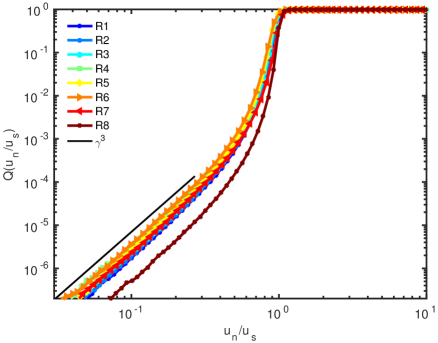
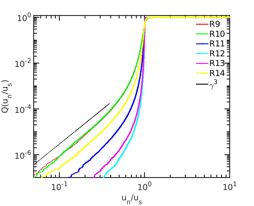
Figure 1: (Color online) Log-Log plots (for runs $R1-R8$) of (a) the complementary cumulative probability distribution function $(Q(\gamma))$ of $(\gamma)=\frac{u_{n}}{u_{s}}$, the ratio of the normal fluid speed and the superfluid speed, for $\gamma\ll 1$, where $Q(\gamma)\sim\gamma^{3}$, (b) and the CPDF $(Q(\gamma))$, for $\gamma\gg 1$, where $Q(\gamma)\sim\gamma^{-3}$, and (c) and the probability distribution function (PDF) $P(\theta)$ of the angle $\theta$ between the normal-fluid velocity and the superfluid velocity; for $\theta\ll\theta_{*},\,P(\theta)\sim\theta$ and for $\theta_{*}\ll\theta\ll 1,\,P(\theta)\sim\theta^{-4}$; (d), (e), and (f) are similar to (a), (b), and (c), respectively (for the runs $R9-R14$ with temperature-dependent viscosities (Table 1).

To obtain the scaling forms of the PDF $P(\theta)$ at small and large values of $\theta$ (Fig. 1 (c)) we note that $\sin{\theta}=\frac{w_{\perp}}{u_{\rm n}}$ (inset of Fig. 1 (c)), where ${\bf w}={\bf u}_{\rm n}-{\bf u}_{\rm s}$ and $w_{\perp}=u_{{\rm n}_{\perp}}$. For $\theta\ll 1$, $\sin{\theta}\sim\theta$ and $u_{{\rm n}_{\perp}}=a_{{\rm n}_{\perp}}t_{\rm n}$; here, $t_{\rm n}\ll 1$ and $a_{{\rm n}_{\perp}}$ is the normal component of the acceleration of the normal fluid. Clearly,

$$P(\theta)=\int\int du_{\rm n}da_{{\rm n}_{\perp}}\delta(\theta-\frac{a_{{\rm n}_{\perp}t_{\rm n}}}{u_{\rm n}})\mathcal{P}(u_{\rm n},a_{{\rm n}_{\perp}}),$$ (29)

where $\mathcal{P}(u_{\rm n},a_{{\rm n}_{\perp}})$ is the joint PDF of $u_{\rm n}$ and $a_{{\rm n}_{\perp}}$. We now make the approximation

$$\mathcal{P}(u_{\rm n},a_{{\rm n}_{\perp}})\sim P(u_{\rm n})P(a_{{\rm n}_{\perp}}),$$ (30)

which can be justified within the framework of the Kolmogorov theory of 1941 (K41) frisch1995turbulence as follows (our arguments follow those in Ref. bhatnagar2016deviation , which obtains the PDF of the angle between the Eulerian velocity of a turbulent fluid and the velocity of an inertial particle that is advected by this fluid): K41 assumes that, in a homogeneous, isotropic, and statistically steady turbulent flow, the only large-length-scale property that is of importance at small length scales is $\epsilon$, the rate of energy dissipation. Viscous dissipation becomes significant at length scales smaller than the K41 dissipation scale $\eta_{d}=[\nu^{3}/\epsilon]^{1/4}$; at such scales the typical fluid acceleration is $a_{*}=\epsilon^{3/4}\nu^{-1/4}$, whereas the dissipation-scale velocity $u_{\eta_{d}}=(\epsilon\nu)^{1/4}$. In the large-Reynolds-number limit, i.e., $\nu\to 0$, in a 3D turbulent fluid, $\epsilon$ goes to a positive constant (the dissipative anomaly); therefore, $a_{*}$ is much larger than typical accelerations because of large-scale fluid motion; by contrast, $u_{\eta_{d}}$ is much smaller than large-scale velocities. In summary, the normal component of the fluid acceleration can be large at small scales, where it is determined, principally, by small-scale properties of the flow; in contrast, dominant fluid velocities are determined by large-scale motions. The separation of length scales in the K41 theory then suggests that, to a good approximation, $a_{*}$ and $u_{\eta_{d}}$ are statistically independent, so their JPDF can be approximated by the product of their respective PDFs. This argument can be applied, mutatis mutandis, to the normal fluid in 3D HVBK turbulence to justify Eq. (30).

We have noted above that, in the HVBK model, $P(u_{\rm n})$ is very well approximated by the Maxwellian distribution $P(u_{\rm n})=C_{\rm n}u_{\rm n}^{d-1}\exp(\frac{-u_{\rm n}^{2}}{2\sigma^{2}})$; our numerical data are consistent with $P(a_{{\rm n}_{\perp}})=B_{1}a_{{\rm n}_{\perp}}^{d-2}\exp({-B_{2}a_{{\rm n}_{\perp}}^{2}})$, where $C_{\rm n},B_{1}$, and $B_{2}$ are constants (this PDF has a similar form in classical-fluid turbulence  bhatnagar2016deviation ). If we use these forms for $P(u_{\rm n})$ and $P(a_{{\rm n}_{\perp}})$, along with Eqs. (29) and (30), and then integrate over $u_{\rm n}$, we get

$$P(\theta)=\int da_{{\rm n}_{\perp}}t_{\rm n}^{d}C_{\rm n}B_{1}\frac{a_{{\rm n}_{\perp}}^{d+1}}{\theta^{d+1}}\exp({-B_{2}a_{{\rm n}_{\perp}}^{2}})\exp({\frac{-a_{{\rm n}_{\perp}}^{2}t_{\rm n}^{2}}{2\theta^{2}\sigma^{2}}}).$$ (31)

If we define the angular scale $\theta_{*}=\frac{a_{*}t_{\rm n}}{{\sqrt{2}}\sigma}$ and the dimensionless variables $X=\frac{\theta}{\theta_{*}}$ and $Y=\frac{a_{{\rm n}_{\perp}}}{a_{*}}$, then Eq. (31) becomes

$$P(\theta) = \int dYt_{\rm n}^{d}C_{\rm n}B_{1}\frac{Y^{d+1}}{\theta^{d+1}}a_{*}^{d+2}\exp(-B_{2}Y^{2}a_{*}^{2})$$ (32)

$$\times \exp(\frac{-Y^{2}}{X^{2}}).$$

We now consider the ranges (a) $0\leq\theta\ll\theta_{*}$, $X\ll 1$ and (b) $\theta_{*}\ll\theta\ll 1$, $1\ll X$. Case (a): the leading term of Eq. (32) is $P(\theta)\sim\int_{0}^{X}dYt_{n}^{d}C_{n}B_{1}\frac{Y^{d+1}}{\theta^{d+1}}$, which can be simplified to get $P(\theta)\sim\theta^{d/3}$, i.e., $P(\theta)\sim\theta$ in $d=3$ for $0\ll\theta\ll\theta_{*}$. Case (b): In this range $\exp{\frac{-Y^{2}}{X^{2}}}\approx 1$ so Eq. (32) yields $P(\theta)=\theta^{-(d+1)}\int dYt_{\rm n}^{d}C_{\rm n}B_{1}\frac{Y^{d+1}}{a_{*}}^{d+2}\exp(-B_{2}Y^{2}a_{*}^{2})$, whence we get $P(\theta)\sim\theta^{-(d+1)}$, i.e., $P(\theta)\sim\theta^{-4}$ in $d=3$, in the range $\theta_{*}\ll\theta\ll 1$. The power laws in the ranges (a) and (b) are consistent with our numerical results in Fig. 1.

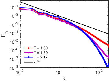
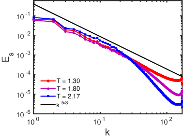
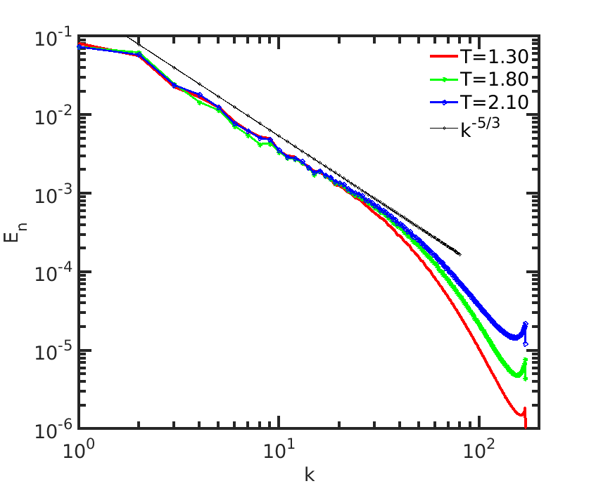
Figure 2: (Color online) Log-Log plots (for $T=1.30$, red lines, $T=1.80$ magenta lines, and $T=2.17$ blue lines) versus the wavenumber $k$ of (a) the energy spectrum $E_{\rm n}(k)$, for the normal fluid, (b) the energy spectrum $E_{\rm s}(k)$, for the superfluid [the black lines indicate the Kolmogorov 1941 (K41) scaling form $\sim k^{-5/3}$], (c) the energy flux $(\Pi_{\rm n})(k)$, for the normal fluid, (d) the energy flux $(\Pi_{\rm s})(k)$, for the superfluid, (e) the absolute value of the real component of the mutual-friction transfer $(\left|Re(\rho_{\rm s}{\bf f}_{mf}\cdot{\bf u}_{\rm n})\right|)$, for the normal fluid, and $(f)$ the absolute value of the real component of the mutual-friction transfer $(\left|Re(\rho_{\rm n}{\bf f}_{mf}\cdot{\bf u}_{\rm s})\right|)$, for the superfluid. (g), (h), and (i) are similar to (a), (c), and (e), respectively, but for the runs $R9,R12$, and $R14$ with temperature-dependent viscosities (Table 1).

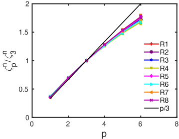
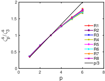
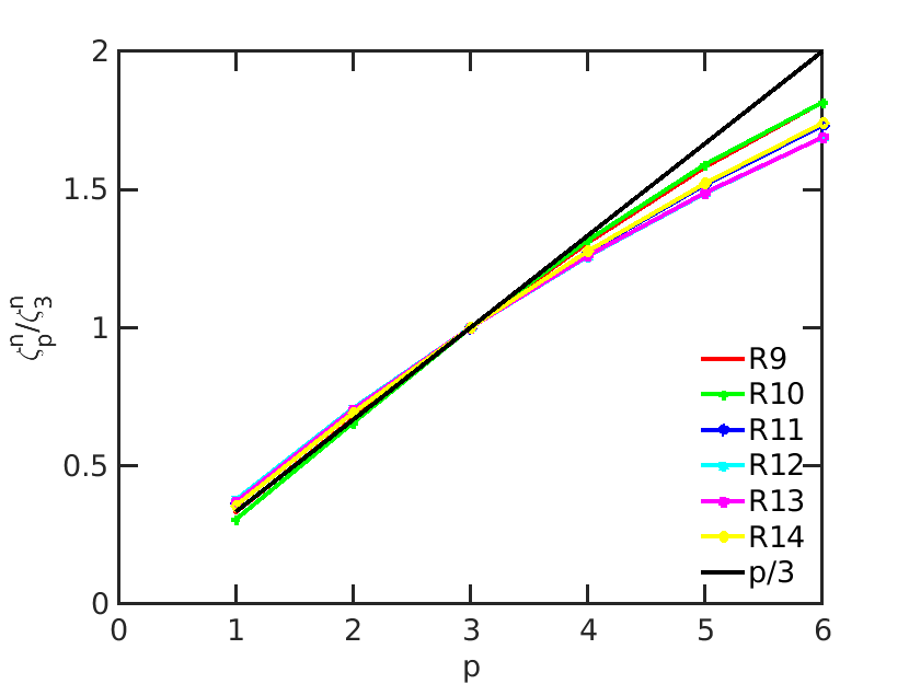
Figure 3: (Color online) Plots versus the order $p$ of the longitudinal-structure-function exponent ratios (a) for the normal fluid $({\zeta_{p}^{\rm n}}/{\zeta_{3}^{\rm n}})$ and (b) for the superfluid $({\zeta_{p}^{\rm s}}/{\zeta_{3}^{\rm s}})$ for runs $R1-R8$; $1\leq p\leq 6$; and we use the extended-self-similarity (ESS) method. Plots of these ratios versus the temperature $T$ for (c) the normal fluid and (d) the superfluid and $p=1$ (red lines), $p=2$ (green lines), $p=3$ (blue lines), $p=4$ (yellow lines), $p=5$ (pink lines), and $p=6$ (cyan lines); the dashed lines show the K41 predictions. Plots versus $T$ of the intermittency exponents (e) $\mu_{p}^{\rm n}=p/3-\zeta_{p}^{\rm n}/\zeta_{3}^{\rm n}$, for the normal fluid, and (f) $\mu_{p}^{\rm s}=\zeta_{p}^{\rm s}/\zeta_{3}^{\rm s}$ for the superfluid, for $p=5$ (red lines) and $p=6$ (blue lines); (g), (h), and (i) are similar to (a), (c), and (e), respectively, but for the runs $R9-R14$ with temperature-dependent viscosities (Table 1).

In Figs.  2 (a) and (b) we present log-log plots of the energy spectra

$${E}_{\rm n}(k) = \sum_{k-1/2<k^{\prime}<k+1/2}{\bf u}_{\rm n}({\bf k}^{\prime})\cdot{\bf u}_{\rm n}({-\bf k}^{\prime})$$

$${E}_{\rm s}(k) = \sum_{k-1/2<k^{\prime}<k+1/2}{\bf u}_{\rm s}({\bf k}^{\prime})\cdot{\bf u}_{\rm s}({-\bf k}^{\prime})$$ (33)

for the normal fluid and the superfluid, respectively, for $T=1.30$, $T=1.80$, and $T=2.17$; the black lines indicate the Kolmogorov 1941 (K41) scaling form $\sim k^{-5/3}$. Figure 2 (g) shows log-log plots versus $k$ of the energy spectrum $E_{n}(k)$; this is similar to Fig.  2 (a), but for the runs with temperature dependent viscosities (Table 1). Figure 2 (g) shows that the tails of the spectra move up as we increase the temperature; this is similar to the results for these spectra in Ref. biferale2018turbulent . In Figs. 2 (c) and (d) we present log-log plots of the energy-flux spectra

$$\Pi_{\rm n} = \bigg{\langle}\int_{k}^{k_{\text{max}}}\mathcal{T}_{\rm n}(k^{\prime},t)dk^{\prime}\bigg{\rangle},$$

$$\Pi_{\rm s} = \bigg{\langle}\int_{k}^{k_{\text{max}}}\mathcal{T}_{\rm s}(k^{\prime},t)dk^{\prime}\bigg{\rangle},$$ (34)

for the normal fluid and the superfluid, respectively. Fig. 2 (h) is similar to Fig. 2 (c) but for the runs with temperature dependent viscosities (Table 1); the constant-energy-flux parts of these plots indicate the extents of the inertial ranges in our DNSs for $T=1.30$, $T=1.80$, and $T=2.17$. Here, $\mathcal{T}_{\rm n}(k^{\prime},t)$ and $\mathcal{T}_{\rm s}(k^{\prime},t)$ are energy-transfer terms in Fourier space because of the triadic interactions in the normal fluid and superfluid, respectively. The parameters for these runs are given in Table 1; we have taken the dependence of $B,\,B^{\prime}$, and $\rho_{n}/\rho_{s}$ on the temperature $T$ from the measurements of Ref. barenghi1983mfriction on superfluid ⁴He; therefore, our results are applicable to measurements of the statistical properties of superfluid turbulence in this system. In Figs. 2 (e) and (f) we present log-log plots of the absolute values of the real part of the mutual-friction transfer terms

$$\mathcal{M}_{\rm n}(k,t) = \sum_{k-1/2<k^{\prime}<k+1/2}\rho_{\rm s}{\bf f}_{\text{mf}}({\bf k}^{\prime})\cdot{\bf u}_{\rm n}({-\bf k}^{\prime}),$$

$$\mathcal{M}_{\rm s}(k,t) = \sum_{k-1/2<k^{\prime}<k+1/2}\rho_{\rm n}{\bf f}_{\text{mf}}({\bf k}^{\prime})\cdot{\bf u}_{\rm n}({-\bf k}^{\prime}),$$ (35)

for the normal-fluid and superfluid components, respectively. We observe that, if we increase the temperature, the mutual-friction transfer for the superfluid increases.

The longitudinal velocity structure functions are

$$S_{p}^{\alpha}(l)=\left\langle\left|\big{(}{\bf u}_{\alpha}({\bf r}+{\bf l})-{\bf u}_{\alpha}({\bf r})\big{)}\cdot\bf{\hat{l}}\right|^{p}\right\rangle;$$ (36)

here, $\alpha=$ n or s, for the normal fluid and superfluid, respectively. In the inertial range $\eta_{d}\ll l\ll L$, $S_{p}^{\alpha}(l)\sim l^{\zeta_{p}^{\alpha}}$; we can use this scaling form to extract the exponents $\zeta_{p}^{\alpha}$ from $S_{p}^{\alpha}(l)$. Furthermore, we can extend the scaling range by using the extended-self-similarity (ESS) method pandit2017overview ; dhar1997some ; benzi1993extended ; chakraborty2010extended to calculate the exponent ratio $\zeta_{p}^{\alpha}/\zeta_{3}^{\alpha}$ from the inertial-range slopes of log-log plots of $S_{p}^{\alpha}(l)$ versus $S_{3}^{\alpha}(l)$. In Figs. 3 (a) and (b) we plot, respectively, the exponent ratios $\zeta_{p}^{\rm n}/\zeta_{3}^{\rm n}$ and $\zeta_{p}^{\rm s}/\zeta_{3}^{\rm s}$ versus the order $p$ ($p\leq 6$). Figures 3 (c), and (d) show the plots of these exponent ratios versus the temperature $T$; the dashed lines give the K41 result for these exponent ratios; in Table 2 we give the numerical values of these exponents ratios (along with error bars, which we determine by a local-slope analysis). From Figs. 3 (c) and (d), we observe that $\zeta^{\rm n}_{p}/\zeta^{3}_{p}$, $\zeta^{\rm s}_{p}/\zeta^{\rm s}_{3}>p/3$ for $p=1$ to $2$, and $\zeta^{\rm n}_{p}/\zeta^{3}_{p}$, $\zeta^{\rm s}_{p}/\zeta^{\rm s}_{3}<p/3$ for $p=4$ to $6$; these are clear signatures of intermittency in superfluid turbulence. Furthermore, we observe that the values of the ratios $\zeta^{\rm n}_{p}/\zeta^{3}_{p}$ and $\zeta^{\rm s}_{p}/\zeta^{\rm s}_{3}$ differ most from their K41 values in the temperature range $T=1.7$ to $1.9$. We can characterize the intermittency by the exponents (see, e.g., Ref. dhar1997some ) $\mu_{p}^{\rm n}=p/3-\zeta_{6}^{\rm n}$; $\mu_{p}^{\rm s}=p/3-\zeta_{6}^{\rm s}$, for $p=5$ and $6$, which measure the deviation of the $5^{th}-$ and $6^{th}-$order exponents from their K41 values. In Figs. 3 (e) and(f) we plot $\mu_{p}^{\rm n}$, and $\mu_{p}^{\rm s}$, respectively, for $p=5$ (red lines) and $p=6$ (blue lines). From Figs. 3 (e), and (f) we observe that these deviations, and hence the intermittency, are highest in the temperature range $T=1.70$ to $T=1.90$. Figures 3 (g), (h), and (i) are similar to Figs.3 (a), (c), and (e), but for the runs with temperature dependent viscosities (Table 1). Intermittency in superfluid turbulence has also been studied in Refs. salort2011investigation ; rusaouen2017intermittency ; procacciaintermittencyshellmodel ; shukla2016multiscaling ; biferale2018turbulent ; varga2018intermittency experimentally and numerically, by shell-model and DNS studies of 3D HVBK turbulence. As in classical-fluid turbulence, we still lack an ab-initio theory of such intermittency.

Run	${\zeta_{1}^{\rm n}}/{\zeta_{3}^{\rm n}}$	$\zeta_{2}^{\rm n}/{\zeta_{3}^{\rm n}}$	$\zeta_{4}^{\rm n}/{\zeta_{3}^{\rm n}}$	$\zeta_{5}^{\rm n}/{\zeta_{3}^{\rm n}}$	$\zeta_{6}^{\rm n}/{\zeta_{3}^{\rm n}}$	${\zeta_{1}^{\rm s}}/{\zeta_{3}^{\rm s}}$	$\zeta_{2}^{\rm s}/{\zeta_{3}^{\rm s}}$	$\zeta_{4}^{\rm s}/{\zeta_{3}^{\rm s}}$	$\zeta_{5}^{\rm s}/{\zeta_{3}^{\rm s}}$	$\zeta_{6}^{\rm s}/{\zeta_{3}^{\rm s}}$
R1	$0.36\pm 0.00$	$0.70\pm 0.00$	$1.27\pm 0.00$	$1.52\pm 0.00$	$1.75\pm 0.01$	$0.36\pm 0.00$	$0.70\pm 0.00$	$1.27\pm 0.00$	$1.52\pm 0.01$	$1.75\pm 0.01$
R2	$0.37\pm 0.00$	$0.70\pm 0.00$	$1.27\pm 0.00$	$1.52\pm 0.01$	$1.75\pm 0.02$	$0.37\pm 0.00$	$0.70\pm 0.00$	$1.27\pm 0.00$	$1.52\pm 0.02$	$1.74\pm 0.03$
R3	$0.37\pm 0.00$	$0.70\pm 0.00$	$1.27\pm 0.01$	$1.52\pm 0.02$	$1.75\pm 0.04$	$0.37\pm 0.01$	$0.70\pm 0.01$	$1.27\pm 0.02$	$1.51\pm 0.04$	$1.73\pm 0.07$
R4	$0.37\pm 0.00$	$0.71\pm 0.00$	$1.26\pm 0.01$	$1.48\pm 0.01$	$1.68\pm 0.02$	$0.37\pm 0.00$	$0.70\pm 0.00$	$1.26\pm 0.01$	$1.49\pm 0.01$	$1.69\pm 0.02$
R5	$0.37\pm 0.00$	$0.70\pm 0.00$	$1.27\pm 0.01$	$1.51\pm 0.01$	$1.73\pm 0.02$	$0.37\pm 0.00$	$0.70\pm 0.01$	$1.27\pm 0.00$	$1.52\pm 0.01$	$1.74\pm 0.02$
R6	$0.37\pm 0.01$	$0.70\pm 0.01$	$1.26\pm 0.01$	$1.50\pm 0.03$	$1.70\pm 0.05$	$0.37\pm 0.00$	$0.70\pm 0.01$	$1.27\pm 0.01$	$1.50\pm 0.03$	$1.71\pm 0.05$
R7	$0.36\pm 0.00$	$0.69\pm 0.00$	$1.28\pm 0.00$	$1.54\pm 0.01$	$1.77\pm 0.01$	$0.36\pm 0.00$	$0.70\pm 0.00$	$1.27\pm 0.01$	$1.52\pm 0.02$	$1.74\pm 0.04$
R8	$0.36\pm 0.00$	$0.70\pm 0.00$	$1.28\pm 0.00$	$1.52\pm 0.01$	$1.75\pm 0.02$	$0.36\pm 0.00$	$0.70\pm 0.00$	$1.28\pm 0.00$	$1.53\pm 0.01$	$1.75\pm 0.02$
R9	$0.33\pm 0.04$	$0.67\pm 0.03$	$1.31\pm 0.05$	$1.58\pm 0.09$	$1.81\pm 0.14$	$0.35\pm 0.03$	$0.68\pm 0.02$	$1.29\pm 0.03$	$1.56\pm 0.08$	$1.79\pm 0.13$
R10	$0.31\pm 0.03$	$0.66\pm 0.02$	$1.32\pm 0.03$	$1.59\pm 0.07$	$1.82\pm 0.10$	$0.35\pm 0.01$	$0.68\pm 0.01$	$1.29\pm 0.01$	$1.56\pm 0.03$	$1.82\pm 0.05$
R11	$0.36\pm 0.02$	$0.69\pm 0.02$	$1.27\pm 0.02$	$1.52\pm 0.05$	$1.73\pm 0.08$	$0.35\pm 0.02$	$0.69\pm 0.01$	$1.28\pm 0.02$	$1.53\pm 0.04$	$1.76\pm 0.06$
R12	$0.37\pm 0.02$	$0.70\pm 0.02$	$1.26\pm 0.04$	$1.49\pm 0.11$	$1.69\pm 0.2$	$0.37\pm 0.01$	$0.69\pm 0.01$	$1.28\pm 0.01$	$1.53\pm 0.02$	$1.77\pm 0.04$
R13	$0.37\pm 0.02$	$0.70\pm 0.02$	$1.26\pm 0.05$	$1.49\pm 0.12$	$1.70\pm 0.21$	$0.37\pm 0.02$	$0.70\pm 0.02$	$1.26\pm 0.05$	$1.49\pm 0.12$	$1.70\pm 0.21$
R14	$0.36\pm 0.06$	$0.69\pm 0.05$	$1.28\pm 0.07$	$1.52\pm 0.16$	$1.75\pm 0.25$	$0.36\pm 0.02$	$0.69\pm 0.02$	$1.27\pm 0.03$	$1.51\pm 0.07$	$1.72\pm 0.12$

Table 2: The numerical values of the exponent ratios $\zeta_{p}^{\rm n}/\zeta_{3}^{\rm n}$ and $\zeta_{p}^{\rm s}/\zeta_{3}^{\rm s}$, from all our DNSs $R1-R14$ and for $1\leq p\leq 6$, along with error bars, which we determine by a local-slope analysis. To determine these exponent ratios we use the extended-self-similarity (ESS) method (see text).

IV CONCLUSIONS

We have used the generating-functional approach to derive the von Kármán-Howarth relations [Eqs. (22)-(25)] for the 3D HVBK model of superfluid turbulence; and we have shown that the simple von Kármán-Howarth relation, for classical-fluid turbulence, is replaced by four relations here. In particular, we have included the effects of the mutual-friction term (if this term is neglected, our general results reduce to those in Ref. biferale2018turbulent ). Furthermore, we have obtained power-law behaviors for the PDFs $P(\gamma)$ and $P(\theta)$ from our DNS results; we have then shown how these power laws can be understood analytically, if we make reasonable decoupling approximations for certain joint PDFs. The exponents of $P(\gamma)$ for the 2D HVBK case, which have been calculated numerically in Ref. shukla2015homogeneous , are in good agreement with our analytical predictions. These power-law exponents are universal in the sense that they are independent of the mutual-friction coefficients $B$ and $B^{\prime}$ and the temperature $T$; it should be possible to measure them in experiments, such as those conducted in Refs. salort2011investigation ; rusaouen2017intermittency ; varga2018intermittency for superfluid ⁴He.

From our DNSs we have obtained energy, energy-flux, and mutual-friction-function spectra. the longitudinal-structure-function exponents for the normal fluid and the superfluid, as a function of the temperature $T$. We have calculated the ratios of structure-function exponents for the normal fluid and the superfluid, via the ESS method, as a function of $T$, by using the experimentally determined mutual-friction coefficients for superfluid Helium ⁴He donnelly1998omfdata . We have shown that there is an enhancement of intermittency for the normal fluid and the superfluid in the range $1.7\leq T\leq 1.90$; our results should be applicable to, and verifiable in, experiments like those of Refs. salort2011investigation ; rusaouen2017intermittency ; varga2018intermittency ; they are also similar to the intermittency results in the DNSs of Ref. biferale2018turbulent .

Acknowledgments We thank A. Bhatnagar and P.E. Roche for fruitful discussions, CSIR, UGC, DST, SERB, and the National Supercomputing Mission (India) for financial support, and SERC (IISc) for providing computational resources. A.B. thanks the Alexander von Humboldt Stiftung, Germany for partial financial support through the Research Group Linkage Programme (2016).

 

V Appendix

We give below some details of our calculations for the structure-function hierarchy.

The pressure contribution, from the normal fluid, is:

$$\eta_{{\rm n}3}I_{\rm p}=\eta_{{\rm n}3}\bigg{\langle}\bigg{[}{\bm{\lambda}}_{\rm n}\cdot\frac{1}{\rho_{\rm n}}\nabla(\Delta p_{\rm n})\bigg{]}Z_{\rm n}\bigg{\rangle};$$ (37)

$$\eta_{{\rm n}3}I_{\rm p}=\bigg{\langle}\bigg{[}\eta_{{\rm n}2}\eta_{{\rm n}3}\frac{1}{\rho_{\rm n}}\big{(}\nabla(\Delta p_{\rm n})\big{)}_{\parallel}+\eta_{{\rm n}3}^{2}\frac{1}{\rho_{\rm n}}\big{(}\nabla(\Delta p_{\rm n})\big{)}_{\perp}\bigg{]}Z_{\rm n}\bigg{\rangle}.$$ (38)

If we take the derivative $\partial_{\eta_{{\rm n}2}}^{2}\partial_{\eta_{{\rm n}3}}$ of Eq. (38) and the limits $\eta_{{\rm n}2},\eta_{{\rm n}3}\rightarrow 0$, we get

$$\lim_{\eta_{{\rm n}2},\eta_{{\rm n}3}\rightarrow 0}\bigg{(}\partial_{\eta_{{\rm n}2}}^{2}\partial_{\eta_{{\rm n}3}}\big{(}\eta_{{\rm n}3}I_{p}\big{)}\bigg{)}=\frac{1}{\rho_{\rm n}}\bigg{\langle}\Delta u_{{\rm n}_{\parallel}}\big{(}\nabla(\Delta p_{\rm n})\big{)}_{\parallel}\bigg{\rangle}.$$ (39)

By applying the derivative $\partial_{\eta_{{\rm n}3}}^{3}$ on Eq. (38), and after taking the limits $\eta_{{\rm n}2},\eta_{{\rm n}3}\rightarrow 0$, we get

$$\lim_{\eta_{{\rm n}3},\eta_{{\rm n}2}\rightarrow 0}\bigg{(}\partial_{\eta_{{\rm n}2}}^{3}\big{(}\eta_{{\rm n}3}I_{\rm p}\big{)}\bigg{)}=\frac{1}{\rho_{\rm n}}\bigg{\langle}\Delta u_{{\rm n}_{\perp}}\big{(}\nabla(\Delta p_{\rm n})\big{)}_{\perp}\bigg{\rangle}.$$ (40)

The total pressure contribution to the third-order structure function for the normal fluid is

$$\frac{1}{\rho_{\rm n}}\bigg{\langle}\Delta u_{{\rm n}_{\parallel}}\big{(}\nabla(\Delta p_{\rm n})\big{)}_{\parallel}+\Delta u_{{\rm n}_{\perp}}\big{(}\nabla(\Delta p_{\rm n})\big{)}_{\perp}\bigg{\rangle}=\frac{1}{\rho_{\rm n}}\bigg{\langle}\Delta u_{{\rm n}i}\nabla_{i}\Delta p_{\rm n}\bigg{\rangle};$$ (41)

$$\bigg{\langle}\Delta u_{{\rm n}_{\parallel}}\big{(}\nabla(\Delta p_{\rm n})\big{)}_{\parallel}+\Delta u_{{\rm n}_{\perp}}\big{(}\nabla(\Delta p_{\rm n})\big{)}_{\perp}\bigg{\rangle}=\bigg{\langle}u_{{\rm n}i}({\bf x}1)\nabla_{i}p_{\rm n}({\bf x}1)-u_{{\rm n}i}({\bf x}2)\nabla_{i}p_{\rm n}({\bf x}1)-u_{{\rm n}i}({\bf x}1)\nabla_{i}p_{\rm n}({\bf x}2)+u_{{\rm n}i}({\bf x}2)\nabla_{i}p_{\rm n}({\bf x}2)\bigg{\rangle}.$$ (42)

In the RHSs of the above equations, we have contributions from the followng two types of terms: (1) terms at the same point, and (2) terms at two different points. By using the homogeneity condition, we write $\big{\langle}u_{{\rm n}i}({\bf x}1)\nabla_{i}p_{\rm n}({\bf x}1)\big{\rangle}=\nabla_{i}\big{\langle}u_{{\rm n}i}({\bf x}1)p_{\rm n}({\bf x}1)\big{\rangle}.$ From the condition of (statistical) homogeneity, we get $\nabla_{i}\big{\langle}u_{{\rm n}i}({\bf x}1)p_{\rm n}({\bf x}1)\big{\rangle}=0.$ Similarly, we get $\nabla_{i}\big{\langle}u_{{\rm n}i}({\bf x}2)p_{\rm n}({\bf x}2)\big{\rangle}=0.$ By using the incompressibility condition, we write $\big{\langle}u_{{\rm n}i}({\bf x}1)\nabla_{i}p_{\rm n}({\bf x}2)\big{\rangle}=\nabla_{i}({\bf x}1)\big{\langle}u_{{\rm n}i}({\bf x}1)p_{\rm n}({\bf x}2)\big{\rangle}=0.$ We define ${\bf r}={\bf x}1-{\bf x}2$ and this gives us $\nabla_{i}({\bf r})=\nabla_{i}({x}1)$. If we apply the homogeneity condition and consider that $\big{\langle}u_{{\rm n}i}({\bf x}1)p_{\rm n}({\bf x}2)\big{\rangle}=A(r)\frac{r_{i}}{r}$, then the physical solution of $\nabla_{i}({\bf x}_{1})\big{(}A(r)\frac{r_{i}}{r}\big{)}=0$ is $A(r)=0$. Thus, $\big{\langle}u_{ni}({\bf x}1)p({\bf x}2)\big{\rangle}=0$; similarly, we can get $\big{\langle}u_{{\rm n}i}({\bf x}2)p({\bf x}1)\big{\rangle}=0$. Now Eq. (42) becomes

$$\bigg{\langle}\Delta u_{{\rm n}_{\parallel}}\big{(}\nabla(\Delta p_{\rm n})\big{)}_{\parallel}\bigg{\rangle}+\bigg{\langle}\Delta u_{{\rm n}_{\perp}}\big{(}\nabla(\Delta p_{\rm n})\big{)}_{\perp}\bigg{\rangle}=0.$$ (43)

The contribution from the perpendicular component in the above equation can be written as $\big{\langle}\Delta u_{{\rm n}_{\perp}}\big{(}\nabla(\Delta p_{\rm n})\big{)}_{\perp}\big{\rangle}=\big{\langle}\Delta u_{{\rm n}_{\theta}}\frac{1}{r}\frac{\partial}{\partial\theta}\Delta p_{\rm n}\big{\rangle}.$ The term $\big{(}\Delta u_{{\rm n}_{\theta}}\frac{1}{r}\frac{\partial}{\partial\theta}\Delta p_{\rm n}\big{)}$ changes its sign under the replacement $\theta\rightarrow-\theta$, hence $\big{\langle}\Delta u_{{\rm n}_{\theta}}\frac{1}{r}\frac{\partial}{\partial\theta}\Delta p_{\rm n}\big{\rangle}=0.$ Furthermore, it implies that $\big{\langle}\Delta u_{{\rm n}_{\parallel}}\big{(}\nabla(\Delta p_{\rm n})\big{)}_{\parallel}\big{\rangle}=\big{\langle}\Delta u_{{\rm n}_{\perp}}\big{(}\nabla(\Delta p_{\rm n})\big{)}_{\perp}\big{\rangle}=0.$ Similarly, we can show that pressure contribution from the superfluid components is also zero, i.e., $\big{\langle}\Delta u_{{\rm s}_{\parallel}}\big{(}\nabla(\Delta p_{\rm s})\big{)}_{\parallel}\big{\rangle}=\big{\langle}\Delta u_{{\rm s}_{\perp}}\big{(}\nabla(\Delta p_{\rm s})\big{)}_{\perp}\big{\rangle}=0.$ Thus, the pressure term does not contribute to the third-order structure functions.

The dissipation term for normal fluid is given as

$$D_{\rm n}=\Big{\langle}\nu_{\rm n}\Big{[}{\bm{\lambda}}_{{\rm n}1}\cdot\nabla^{2}_{{\bf x}_{1}}{\bf u}_{\rm n}{({\bf x}_{1})}+{\bm{\lambda}}_{{\rm n}2}\cdot\nabla^{2}_{{\bf x}_{2}}{\bf u}_{\rm n}{({\bf x}_{2})}\Big{]}Z_{\rm n}\Big{\rangle}.$$ (44)

For convenience, we consider that ${\bm{\lambda}}_{{\rm n}1}=-{\bm{\lambda}}_{{\rm n}2}$ and ${\bm{\lambda}}_{{\rm s}1}=-{\bm{\lambda}}_{{\rm s}2}$; and for notational simplicity we consider ${\bm{\lambda}}_{{\rm n}1}={\bm{\lambda}}_{\rm n}$ and ${\bm{\lambda}}_{{\rm s}1}={\bm{\lambda}}_{\rm s}$. In terms of ${\bm{\lambda}}_{\rm n}$ and ${\bm{\lambda}}_{\rm s}$ the dissipation terms are

$$D_{\rm n}=\Big{\langle}\nu_{\rm n}\Big{[}{\bm{\lambda}}_{\rm n}\cdot\nabla^{2}_{{\bf x}_{1}}{\bf u}_{\rm n}{({\bf x}_{1})}-{\bm{\lambda}}_{\rm n}\cdot\nabla^{2}_{{\bf x}_{2}}{\bf u}_{\rm n}{({\bf x}_{2})}\Big{]}Z_{\rm n}\Big{\rangle};$$ (45)

$$D_{\rm n}=\nu_{\rm n}\Big{\langle}\Big{[}\eta_{{\rm n}2}\nabla^{2}_{{\bf x}_{1}}{\bf u}_{{\rm n}_{\parallel}}{({\bf x}_{1})}-\eta_{{\rm n}2}\nabla^{2}_{{\bf x}_{2}}{\bf u}_{{\rm n}_{\parallel}}{({\bf x}_{2})}+\eta_{{\rm n}3}\nabla^{2}_{{\bf x}_{1}}{\bf u}_{{\rm n}_{\perp}}{({\bf x}_{1})}-\eta_{{\rm n}3}\nabla^{2}_{{\bf x}_{2}}{\bf u}_{{\rm n}_{\perp}}{({\bf x}_{2})}\Big{]}Z_{\rm n}\Big{\rangle}.$$ (46)

We note that

$$\Big{\langle}\nu_{\rm n}\Big{(}\nabla^{2}_{{\bf x}_{1}}+\nabla^{2}_{{\bf x}_{2}}\Big{)}Z_{\rm n}\Big{\rangle}=\nu_{\rm n}\langle\Big{[}\eta_{{\rm n}2}\nabla^{2}_{{\bf x}_{1}}{\bf u}_{{\rm n}_{\parallel}}{({\bf x}_{1})}-\eta_{{\rm n}2}\nabla^{2}_{{\bf x}_{2}}{\bf u}_{{\rm n}_{\parallel}}{({\bf x}_{2})}+\eta_{{\rm n}3}\nabla^{2}_{{\bf x}_{1}}{\bf u}_{{\rm n}_{\perp}}{({\bf x}_{1})}-\eta_{{\rm n}3}\nabla^{2}_{{\bf x}_{2}}{\bf u}_{{\rm n}_{\perp}}{({\bf x}_{2})}\Big{]}Z_{\rm n}\Big{\rangle}+$$

$$+\nu_{\rm n}\Big{\langle}Z_{\rm s}\Big{[}\eta_{{\rm n}2}\nabla_{{\bf x}_{1}}{\bf u}_{{\rm n}_{\parallel}}{({\bf x}_{1})}+\eta_{{\rm n}3}\nabla_{{\bf x}_{1}}{\bf u}_{{\rm n}_{\perp}}{({\bf x}_{1})}\Big{]}^{2}Z_{\rm n}\Big{\rangle}+\nu_{\rm n}\Big{\langle}Z_{\rm s}\Big{[}\eta_{{\rm n}2}\nabla_{{\bf x}_{2}}{\bf u}_{{\rm n}_{\parallel}}{({\bf x}_{2})}+\eta_{{\rm n}3}\nabla_{{\bf x}_{2}}{\bf u}_{{\rm n}_{\perp}}{({\bf x}_{2})}\Big{]}^{2}Z_{\rm n}\Big{\rangle};$$ (47)

by substituting the value of $D_{\rm n}$ in this equation, we get

$$\Big{\langle}\nu_{\rm n}\Big{(}\nabla^{2}_{{\bf x}_{1}}+\nabla^{2}_{{\bf x}_{2}}\Big{)}Z_{\rm n}\Big{\rangle}=D_{\rm n}+\nu_{\rm n}\Big{\langle}\Big{[}\eta_{{\rm n}2}^{2}\Big{(}\nabla_{{\bf x}_{1}}{\bf u}_{{\rm n}_{\parallel}}{({\bf x}_{1})}\Big{)}^{2}+\eta_{{\rm n}3}^{2}\Big{(}\nabla_{{\bf x}_{1}}{\bf u}_{{\rm n}_{\perp}}{({\bf x}_{1})}\Big{)}^{2}+2\eta_{{\rm n}2}\eta_{{\rm n}3}\Big{(}\nabla_{{\bf x}_{1}}{\bf u}_{{\rm n}_{\parallel}}{({\bf x}_{1})}\Big{)}\Big{(}\nabla_{{\bf x}_{1}}{\bf u}_{{\rm n}_{\perp}}{({\bf x}_{1})}\Big{)}\Big{]}Z_{\rm n}\Big{\rangle}$$

$$+\nu_{\rm n}\Big{\langle}\Big{[}\eta_{{\rm n}2}^{2}\Big{(}\nabla_{{\bf x}_{2}}{\bf u}_{{\rm n}_{\parallel}}{({\bf x}_{2})}\Big{)}^{2}+\eta_{{\rm n}3}^{2}\Big{(}\nabla_{{\bf x}_{2}}{\bf u}_{{\rm n}_{\perp}}{({\bf x}_{2})}\Big{)}^{2}+2\eta_{{\rm n}2}\eta_{{\rm n}3}\Big{(}\nabla_{{\bf x}_{2}}{\bf u}_{{\rm n}_{\parallel}}{({\bf x}_{2})}\Big{)}\Big{(}\nabla_{{\bf x}_{2}}{\bf u}_{{\rm n}_{\perp}}{({\bf x}_{2})}\Big{)}\Big{]}Z_{\rm n}\Big{\rangle}.$$ (48)

On using $\nu_{\rm n}\Big{(}\nabla_{{\bf a}}{\bf u}_{{\rm n}_{\parallel}}{({\bf a})}\Big{)}^{2}=\epsilon_{{\rm n}_{\parallel}}({\bf a})$ and $\nu_{\rm n}\Big{(}\nabla_{{\bf a}}{\bf u}_{{\rm n}_{\perp}}{({\bf a})}\Big{)}^{2}=\epsilon_{{\rm n}_{\perp}}({\bf a})$, where ${\bf a}$ stands for ${\bf x}_{1}$ or ${\bf x}_{2}$, we get the following:

$$\Big{\langle}\nu_{\rm n}\Big{(}\nabla^{2}_{{\bf x}_{1}}+\nabla^{2}_{{\bf x}_{2}}\Big{)}Z_{\rm n}\Big{\rangle}=D_{\rm n}+\Big{\langle}\Big{[}\eta_{{\rm n}2}^{2}\Big{(}\epsilon_{{\rm n}_{\parallel}}({\bf x}_{1})+\epsilon_{{\rm n}_{\parallel}}({\bf x}_{2})\Big{)}+\eta_{{\rm n}3}^{2}\Big{(}\epsilon_{{\rm n}_{\perp}}({\bf x}_{1})+\epsilon_{{\rm n}_{\perp}}({\bf x}_{2})\Big{)}\Big{]}Z_{\rm n}\Big{\rangle}$$

$$+2\Big{\langle}\eta_{{\rm n}2}\eta_{{\rm n}3}\Big{[}\Big{(}\epsilon_{{\rm n}_{\parallel}}{({\bf x}_{1})}\epsilon_{{\rm n}_{\perp}}{({\bf x}_{1})}\Big{)}^{\frac{1}{2}}\Big{(}\epsilon_{{\rm n}_{\parallel}}{({\bf x}_{2})}\epsilon_{{\rm n}_{\perp}}{({\bf x}_{2})}\Big{)}^{\frac{1}{2}}\Big{]}Z_{\rm n}\Big{\rangle}.$$ (49)

If we take the limit $\nu_{\rm n}\rightarrow 0$ and set $\epsilon_{{\rm n}_{\parallel}}({\bf x}_{1})+\epsilon_{{\rm n}_{\parallel}}({\bf x}_{2})=\epsilon_{{\rm n}_{\parallel}}$ and $\epsilon_{{\rm n}_{\perp}}({\bf x}_{1})+\epsilon_{{\rm n}_{\perp}}({\bf x}_{2})=\epsilon_{{\rm n}_{\perp}}$, in the above equation, we get

$$0= D_{\rm n}+\Big{\langle}\Big{[}\eta_{{\rm n}2}^{2}\epsilon_{{\rm n}_{\parallel}}+\eta_{{\rm n}3}^{2}\epsilon_{{\rm n}_{\perp}}\Big{]}Z_{\rm n}\Big{\rangle}+2\Big{\langle}\eta_{{\rm n}2}\eta_{{\rm n}3}\Big{[}\Big{(}\epsilon_{{\rm n}_{\parallel}}{({\bf x}_{1})}\epsilon_{{\rm n}_{\perp}}{({\bf x}_{1})}\Big{)}^{\frac{1}{2}}+\Big{(}\epsilon_{{\rm n}_{\parallel}}{({\bf x}_{2})}\epsilon_{{\rm n}_{\perp}}{({\bf x}_{2})}\Big{)}^{\frac{1}{2}}\Big{]}Z_{\rm n}\Big{\rangle};$$ (50)

or

$$-D_{\rm n}= \Big{\langle}\Big{[}\eta_{{\rm n}2}^{2}\epsilon_{{\rm n}_{\parallel}}+\eta_{{\rm n}3}^{2}\epsilon_{{\rm n}_{\perp}}]Z_{\rm n}\Big{\rangle}+2\Big{\langle}\eta_{{\rm n}2}\eta_{{\rm n}3}\Big{[}\Big{(}\epsilon_{{\rm n}_{\parallel}}{({\bf x}_{1})}\epsilon_{{\rm n}_{\perp}}{({\bf x}_{1})}\Big{)}^{\frac{1}{2}}+\Big{(}\epsilon_{{\rm n}_{\parallel}}{({\bf x}_{2})}\epsilon_{{\rm n}_{\perp}}{({\bf x}_{2})}\Big{)}^{\frac{1}{2}}\Big{]}Z_{\rm n}\Big{\rangle}.$$ (51)

Similarly, the dissipation term from the superfluid part is

$$-D_{\rm s}= \Big{\langle}\Big{[}\eta_{{\rm s}2}^{2}\epsilon_{{\rm s}_{\parallel}}+\eta_{{\rm s}3}^{2}\epsilon_{{\rm s}_{\perp}}]Z_{\rm s}\Big{\rangle}+2\Big{\langle}\eta_{{\rm s}2}\eta_{{\rm s}3}\Big{[}\Big{(}\epsilon_{{\rm s}_{\parallel}}{({\bf x}_{1})}\epsilon_{{\rm s}_{\perp}}{({\bf x}_{1})}\Big{)}^{\frac{1}{2}}+\Big{(}\epsilon_{{\rm s}_{\parallel}}{({\bf x}_{2})}\epsilon_{{\rm s}_{\perp}}{({\bf x}_{2})}\Big{)}^{\frac{1}{2}}\Big{]}Z_{\rm s}\Big{\rangle}.$$ (52)

References

- (1) U. Frisch, and A. N. Kolmogorov, Turbulence: the legacy of AN Kolmogorov (Cambridge University Press, Cambridge, UK, 1995).
- (2) R. Pandit, P. Perlekar, and S. S. Ray, Pramana 73, 157 (2009).
- (3) G. Boffetta, A. Mazzino, and A. Vulpiani, J. Phys. A: Mathematical and Theoretical 41, 363001 (2008).
- (4) G. Boffetta and R. E. Ecke, Ann. Rev. Fluid Mech. 44, 427 (2012).
- (5) R. J. Donnelly and C. F. Barenghi, J. Phys. Chem. Ref. Data 27, 1217 (1998).
- (6) J. Maurer and P. Tabeling, Europhys. Lett. 43, 29 (1998).
- (7) M. S. Paoletti and D. P. Lathrop, Annu. Rev. Condens. Matter Phys. 2, 213 (2011).
- (8) G. P. Bewley, D. P. Lathrop, and K. R. Sreenivasan, Nature 441, 588 (2006).
- (9) E. A. L. Henn, A. J. Seman, G. Roati, K. M. F. Magalhães, and V. S. Bagnato, Phys. Rev. Lett. 103, 045301 (2009).
- (10) P. E. Roche, P Diribarne, T. Didelot, O. Français, L. Rousseau, and H. Willaime, Europhys. Lett. 77, 66002 (2007).
- (11) W. Guo, S. B. Cahn, J. A. Nikkel, W. F. Vinen, and D. N. McKinsey, Phys. Rev. Lett. 105, 045301 (2010).
- (12) W. Guo, M. La Mantia, D. P. Lathrop, and S. W. Van Sciver, Proc. Natl. Acad. Sci. USA 111, 4653 (2014).
- (13) J. Salort, B. Chabaud, E. Lévêque, and P.-E. Roche, in J. Phys. Conf. Ser. Vol. 318, p. 042014.
- (14) N. G. Berloff, M. Brachet, and N. P. Proukakis, Proc. Natl. Acad. Sci. USA 111, 4675 (2014).
- (15) V. S. Lvov, S. V. Nazarenko, and L. Skrbek, J. Low Temp. Phys. 145, 125 (2006).
- (16) S. K. Nemirovskii, Phys. Reports 524, 85 (2013).
- (17) V. Shukla, A. Gupta, and R. Pandit, Phys. Rev. B 92, 104510 (2015).
- (18) M. Kobayashi and M. Tsubota, Phys. Rev. Lett. 94, 065302 (2005).
- (19) L. Boué, V. L’vov, A. Pomyalov, and I. Procaccia, Phys. Rev. B 85, 104502 (2012).
- (20) D. I. Bradley, D. O. Clubb, S. N. Fisher, A. M. Guenault, R. P. Haley, C. J. Matthews, G. R. Pickett, V. Tsepelin, and K. Zaki, Phys. Rev. Lett. 96, 035301 (2006).
- (21) N. Parker and C. Adams, Phys. Rev. Lett. 95, 145301 (2005).
- (22) M. Kobayashi and M. Tsubota, Phys. Rev. A 76, 045603 (2007).
- (23) E. Zaremba, T. Nikuni, and A. Griffin, J. Low Temp. Phys. 116, 277 (1999).
- (24) C. Nore, M. Abid, and M. Brachet, Phys. Rev. Lett. 78, 3896 (1997).
- (25) V. Shukla, M. Brachet, and R. Pandit, New J. Phys. 15, 113025 (2013).
- (26) G. Krstulovic and M. Brachet, Phys. Rev. E 83, 066311 (2011).
- (27) K. Schwarz, Phys. Rev. B 31, 5782 (1985).
- (28) K. Schwarz, Phys. Rev. B 38, 2398 (1988).
- (29) R. Hänninen and A. W. Baggaley, Proc. Natl. Acad. Sci. USA 111, 4667 (2014)
- (30) L. Landau, Phys. Rev. 60, 356 (1941).
- (31) L. Tisza, Phys. Rev. 72, 838 (1947).
- (32) C. F. Barenghi, Phys. Rev. B 45, 2290 (1992).
- (33) P. E. Roche, C. F. Barenghi, and E. Lévêque, Europhys. Lett. 87, 54006 (2009).
- (34) W. Vinen and J. Niemela, J. Low Temp. Phys. 128, 167 (2002).
- (35) G. V. Kolmakov, P. V. E. McClintock, and S. V. Nazarenko, Proc. Natl. Acad. Sci. USA 111, 4727 (2014).
- (36) E. Kozik and B. Svistunov, Phys. Rev. Lett. 92, 035301 (2004).
- (37) V. S. Lvov and S. Nazarenko, JETP Letters 91, 428 (2010).
- (38) J. Salort, P. E. Roche, and E. Lévêque, Europhys. Lett. 94, 24001 (2011).
- (39) J. Salort, B. Chabaud, E. Lévêque, and P.-E. Roche, Eu- rophys. Lett. 97, 34006 (2012).
- (40) E. Rusaouen, B. Chabaud, J. Salort, and P.-E. Roche, Phys. Fluids 29, 105108 (2017).
- (41) E. Varga, J. Gao, W. Guo, and L. Skrbek, Phys. Rev. Fluids 3, 094601 (2018).
- (42) L. Boué, V. L’vov, A. Pomyalov, and I. Procaccia, Phys. Rev. Lett. 110, 014502 (2013).
- (43) V. Shukla and R. Pandit, Phys. Rev. E 94, 043101 (2016).
- (44) L. Biferale, D. Khomenko, V. L’vov, A. Pomyalov, I. Procaccia, and G. Sahoo, Phys. Rev. Fluids 3, 024605 (2018).
- (45) A. M. Polyakov, Phys. Rev. E 52, 6183 (1995).
- (46) V. Yakhot, Phys. Rev. E 63, 026307 (2001).
- (47) A. Basu, A. Naji, and R. Pandit, Phys. Rev. E 89, 012117 (2014).
- (48) C. F. Barenghi, R. J. Donnelly, and W. F. Vinen, J. Low Temp. Phys. 52, 189 (1983).
- (49) V. S. L’vov, S. V. Nazarenko, and O. Rudenko, Phys. Rev. B 76, 024520 (2007).
- (50) K. Morris, J. Koplik, and D. W. I. Rouson, Phys. Rev. Lett. 101, 015301 (2008).
- (51) D. H. Wacks and C. F. Barenghi, Phys. Rev. B 84, 184505 (2011).
- (52) C. Canuto, M. Y. Hussaini, A. Quarteroni, and T. A. Zang,Spectral Methods: Fundamentals in Single Do- mains (Springer, 2006).
- (53) A. Lamorgese, D. Caughey, and S. Pope, Phys. Fluids 17, 015106 (2005).
- (54) G. Sahoo, P. Perlekar, and R. Pandit, New J. Phys. 13, 013036 (2011).
- (55) W. Woyczynski, Burgers-KPZ Turbulence-Gottingen Lectures (Springer-Verlag, Berlin, Heidelberg, 1998).
- (56) W. McComb, The Phys. of Fluid Turbulence (Claredon Press, Oxford, 1990).
- (57) L. Boué, V. L’vov, Y. Nagar, S. V. Nazarenko, A. Pomyalov, and I. Procaccia, Phys. Rev. B 91, 144501 (2015).
- (58) R. Pandit, D. Banerjee, A. Bhatnagar, M. Brachet, A. Gupta, D. Mitra, N. Pal, P. Perlekar, S. S. Ray, V. Shukla, and D. Vincenzi, Phys. fluids 29, 111112 (2017).
- (59) S. K. Dhar, A. Sain, A. Pande, and R. Pandit, Pramana 48, 325 (1997).
- (60) A. Bhatnagar, A. Gupta, D. Mitra, P. Perlekar, M. Wilkinson, R. Pandit, Phys. Rev. E 94, 063112 (2016).
- (61) R. Benzi, S. Ciliberto, R. Tripiccione, C. Baudet, F. Massaioli, and S. Succi, Phys. Rev. E 48, R29 (1993).
- (62) S. Chakraborty, U. Frisch, and S. S. Ray, J. Fluid Mech. 649, 275 (2010).