Abstract

Finite Bose systems cannot display a genuine Bose-Einstein condensate with infinite long-range order. But, if the number of trapped atoms is sufficiently large, a kind of Bose-Einstein condensation does occur, with the properties of the arising quasi-condensate being very close to the genuine condensate. Although the quasi-condensate does not enjoy long-range order, it has mid-range order. This paper shows that the level of mid-range order in finite Bose systems can be characterized by order indices of density matrices.

1 Introduction

Bose-Einstein condensation of trapped atoms has been a hot topic in recent years, intensively investigated both experimentally and theoretically (see, e.g., review articles and books [1, 2, 3, 4, 5, 6, 7, 8, 9, 10, 11, 12, 13, 14, 15, 16, 17, 18, 19]). Trapped atoms represent finite systems. In finite systems, strictly speaking, there can be no phase transitions with arising long-range order. Respectively, there can be no genuine phase transition of Bose-Einstein condensation in a finite trap. Nevertheless, when a finite system is sufficiently large, its properties can be so close to a bulk system that, with a good approximation, one can speak of phase transitions there. In that sense, one studies Bose-Einstein condensation in finite traps. And one calls the arising quasi-condensate just Bose condensate.

However, it is interesting as to what extent the quasi-condensate in a finite system differs from the genuine condensate. More precisely, how it would be possible to distinguish infinite off-diagonal order, corresponding to the genuine condensate accompanied by spontaneous breaking of global gauge symmetry, from quasi-condensate in a finite system? Is it possible to define a measure quantifying the level of a quasi-long-range order?

In the present paper, we show that the Bose quasi-condensate in a finite system is characterized by mid-range order that can be quantified by order indices.

2 Order indices

Order indices were introduced for density matrices in [20] and considered for several macroscopic systems [21, 22, 23, 24]. The notion of order indices was generalized for arbitrary matrices and operators in [25].

Let an operator $\hat{A}$ acting on a Hilbert space $\mathcal{H}$ possess a finite norm $\|\hat{A}\|$ and a trace. The order index of the operator is defined as

$$\omega(\hat{A})\equiv\frac{\log||\;\hat{A}\;||}{\log|\;{\rm Tr}_{\cal H}\hat{A}\;|}\;.$$ (1)

One says that an operator $\hat{A_{1}}$ is better ordered than $\hat{A_{2}}$ if and only if the order index of $\hat{A_{1}}$ is larger than that of $\hat{A_{2}}$. If their order indices are equal, then one says that these operators are equally ordered. The convenient norm in definition (1) is the Hermitian operator norm

$$||\;\hat{A}\;||=\sup_{\varphi}\;\frac{|\;\hat{A}\varphi\;|}{|\;\varphi\;|}=\sup_{\varphi}\left[\frac{(\hat{A}\varphi,\hat{A}\varphi)}{(\varphi,\varphi)}\right]^{1/2}\;,$$

where $\varphi\in\mathcal{H}$ is not zero. If the operator is Hermitian and $\{\varphi_{k}\}$ is an orthonormal basis in $\mathcal{H}$, then the Hermitian norm reduces to

$$||\;\hat{A}\;||=\sup_{\varphi}\;\frac{|(\varphi,\hat{A}\varphi)|}{|\;\varphi\;|}=\sup_{\varphi_{k}}(\varphi_{k},\hat{A}\varphi_{k})\qquad(\hat{A}^{+}=\hat{A})\;.$$

For a semi-positive operator $\hat{A}\geq 0$ the norm is not larger than the trace, because of which

$$\omega(\hat{A})\leq 1\qquad(\hat{A}\geq 0)\;.$$ (2)

Order indices can be introduced for generalized density matrices as follows. Let $x$ be a set of physical variables and $\mathcal{A}=\{\hat{A}(x)\}$ be the algebra of local observables acting on a Fock space $\mathcal{F}$. And let $\mathcal{A}_{\psi}=\{\hat{\psi}(x),\hat{\psi}^{\dagger}(x)\}$ be the algebra of field operators on $\mathcal{F}$. The union $\mathcal{A}_{ext}\equiv\mathcal{A}\bigoplus\mathcal{A}_{\psi}$ is called the extended local algebra.

For any representative $A(x)$ of the extended local algebra $\mathcal{A}_{ext}$, it is possible to define the averages

$$D_{A}(x_{1},x_{2},\ldots,x_{n};y_{1},y_{2},\ldots,y_{n})\;=$$

$$=\;{\rm Tr}_{\cal F}A(x_{1})A(x_{2})\ldots A(x_{n})\;\hat{\rho}\;A^{+}(y_{n})A^{+}(y_{n-1})\ldots A^{+}(y_{1})\;,$$ (3)

where $\hat{\rho}$ is a statistical operator. These averages can be treated as matrix elements of the matrix

$$\hat{D}_{A}^{n}\equiv[\;D_{A}(x_{1},x_{2},\ldots,x_{n};y_{1},y_{2},\ldots,y_{n})\;]\;,$$ (4)

which can be called a generalized density matrix.

It is also possible to consider the functions $\varphi(x_{1},x_{2},\ldots,x_{n})$ of a Hilbert space $\mathcal{H}_{n}$ as columns

$$\varphi_{n}\equiv[\;\varphi(x_{1},x_{2},\ldots,x_{n})\;]\;.$$ (5)

Then the norm of matrix (4) can be defined as

$$||\;\hat{D}_{A}^{n}\;||=\sup_{\varphi_{n}}\;\frac{(\varphi_{n},\hat{D}_{A}^{n}\varphi_{n})}{(\varphi_{n},\varphi_{n})}\;,$$ (6)

where the scalar product is given by the definition

$$(\varphi_{n},\varphi_{n}^{\prime})=\int\varphi^{*}(x_{1},x_{2},\ldots,x_{n})\varphi_{n}^{\prime}(x_{1},x_{2},\ldots,x_{n})\;\prod_{i=1}^{n}dx_{i}\;.$$

Respectively, the trace of the matrix is

$${\rm Tr}\hat{D}_{A}^{n}=\int D_{A}(x_{1},x_{2},\ldots,x_{n};x_{1},x_{2},\ldots,x_{n})\;\prod_{i=1}^{n}dx_{i}\;.$$ (7)

The order index of the generalized density matrix is

$$\omega(\hat{D}_{A}^{n})\equiv\frac{\log||\;\hat{D}_{A}^{n}\;||}{\log|\;{\rm Tr}\hat{D}_{A}^{n}\;|}\;.$$ (8)

A particular case of the generalized density matrices are the reduced density matrices [26]

$$\hat{\rho}_{n}=\hat{D}_{\psi}^{n}=[\;\rho(x_{1},x_{2},\ldots,x_{n};y_{1},y_{2},\ldots,y_{n})\;]\;,$$ (9)

with the matrix elements

$$\rho(x_{1},x_{2},\ldots,x_{n};y_{1},y_{2},\ldots,y_{n})\;\equiv$$

$$\equiv\;{\rm Tr}_{\cal F}\hat{\psi}(x_{1})\hat{\psi}(x_{2})\ldots\hat{\psi}(x_{n})\;\hat{\rho}\;\hat{\psi}^{\dagger}(y_{n})\hat{\psi}^{\dagger}(y_{n-1})\ldots\hat{\psi}^{\dagger}(y_{1})\;.$$ (10)

The related order index of a density matrix (9) is

$$\omega(\hat{\rho}_{n})\equiv\frac{\log||\;\hat{\rho}_{n}\;||}{\log|\;{\rm Tr}\hat{\rho}_{n}\;|}\;.$$ (11)

If $\varphi_{nk}$ is an eigenfunction, labeled by a multi-index $k$, of the density matrix (9), then its eigenvalues are

$$N_{nk}\equiv(\varphi_{nk},\hat{\rho}_{n}\varphi_{nk})$$ (12)

and its Hermitian norm is

$$||\;\hat{\rho}_{n}\;||=\sup_{k}N_{nk}\;.$$ (13)

Because of the trace

$${\rm Tr}\hat{\rho}_{n}=\frac{N!}{(N-n)!}\;,$$

the order index (11) can be represented in the form

$$\omega(\hat{\rho}_{n})=\frac{\log\sup_{k}N_{nk}}{\log[N!/(N-n)!]}\;.$$ (14)

The norms of the reduced density matrices satisfy [26] the inequalities

$$||\;\hat{\rho}_{n}\;||\;\leq\;(b_{n}N)^{n}\qquad(Bose)$$

for Bose particles and

$$||\;\hat{\rho}_{2n}\;||\;\leq\;(c_{2n}N)^{n}\;,\qquad||\;\hat{\rho}_{2n+1}\;||\;\leq\;(c_{2n+1}N)^{n}\qquad(Fermi)\;,$$

for Fermi particles, where $b_{n}$ and $c_{n}$ are finite numbers. Therefore for the order indices of density matrices, under large $N\gg 1$, we have

$$\omega(\hat{\rho}_{n})\;\leq\;1\qquad(Bose)$$ (15)

for bosons and

$$\omega(\hat{\rho}_{2n})\;\leq\;\frac{1}{2}\;,\qquad\omega(\hat{\rho}_{2n+1})\;\leq\;\frac{n}{2n+1}\qquad(Fermi)$$ (16)

for fermions.

3 Dilute gas

As an example of a concrete finite system, let us consider a dilute Bose gas with local interactions

$$\Phi({\bf r})=\Phi_{0}\delta({\bf r})\;,\qquad\Phi_{0}\equiv 4\pi\;\frac{a_{s}}{m}\;,$$ (17)

in which $m$ is atomic mass and $a_{s}$, scattering length. Here and in what follows, the Planck and Boltzmann constants are set to one, $\hbar=1$ and $k_{B}=1$. The energy Hamiltonian reads as

$$\hat{H}=\int\hat{\psi}^{\dagger}({\bf r})\left(-\;\frac{\nabla^{2}}{2m}\right)\psi({\bf r})\;d{\bf r}\;+\;\frac{1}{2}\;\Phi_{0}\int\hat{\psi}^{\dagger}({\bf r})\hat{\psi}^{\dagger}({\bf r})\hat{\psi}({\bf r})\hat{\psi}({\bf r})\;d{\bf r}\;,$$ (18)

where $\hat{\psi}({\bf r})$ is a Bose field operator, generally depending on time $t$, which is not shown for simplicity of notation.

Below we employ the self-consistent approach, reviewed in [16, 17, 18, 27], guaranteeing the correct description of Bose-condensed systems. This approach possesses several unique features: (i) satisfies all conservation laws; (ii) gives a gapless spectrum; (iii) describes Bose-Einstein condensation as a second order phase transition; (iv) provides for the condensate fraction, as a function of interaction strength, good numerical agreement with Monte Carlo simulations, both for uniform as well as for trapped systems; (v) leads to the behavior of the ground state energy, under varying interaction strength, which, at weak interactions, yields exactly the Lee-Huang-Yang formula [28, 29, 30] and, at strong interactions, it is close to the results of Monte Carlo calculations; (vi) explains the effect of local condensate depletion at trap center under strong interactions [31], agreeing well with Monte Carlo simulations.

We start with the Bogolubov shift [32, 33, 34]

$$\hat{\psi}({\bf r})=\eta({\bf r})+\psi_{1}({\bf r})$$ (19)

separating the condensate (quasi-condensate) function $\eta$ from the field operator of uncondensed atoms $\psi_{1}$, with these quantities being mutually orthogonal,

$$\int\eta^{*}({\bf r})\psi_{1}({\bf r})\;d{\bf r}=0\;.$$ (20)

The condensate function plays the role of an order parameter, so that

$$\eta({\bf r})=\langle\;\hat{\psi}({\bf r})\;\rangle\;,\qquad\langle\;\psi_{1}({\bf r})\;\rangle=0\;.$$ (21)

The total number of atoms $N=N_{0}+N_{1}$ is formed by the number of condensed atoms

$$N_{0}=\int|\;\eta({\bf r})\;|^{2}\;d{\bf r}$$ (22)

and the number of uncondensed atoms

$$N_{1}=\langle\;\hat{N}_{1}\;\rangle\;,\qquad\hat{N}_{1}\equiv\int\psi_{1}^{\dagger}({\bf r})\psi_{1}({\bf r})\;d{\bf r}\;.$$ (23)

The grand Hamiltonian, taking into account conditions (21), (22), and (23), reads as

$$H=\hat{H}-\mu_{0}N_{0}-\mu_{1}\hat{N}_{1}-\hat{\Lambda}\;,$$ (24)

where

$$\hat{\Lambda}=\int[\;\lambda({\bf r})\psi_{1}^{\dagger}({\bf r})+\lambda^{*}({\bf r})\psi_{1}({\bf r})\;]\;d{\bf r}\;.$$

The quantities $\mu_{0}$, $\mu_{1}$, and $\lambda({\bf r})$ are the Lagrange multipliers guaranteeing the validity of these conditions.

Equations of motion, equivalent to the Heisenberg equations [17], are the equation for the condensate fraction

$$i\;\frac{\partial}{\partial t}\;\eta({\bf r},t)=\left\langle\frac{\delta H}{\delta\eta^{*}({\bf r},t)}\right\rangle$$ (25)

and the equation for the field operator of uncondensed atoms

$$i\;\frac{\partial}{\partial t}\;\psi_{1}({\bf r},t)=\frac{\delta H}{\delta\psi_{1}^{\dagger}({\bf r},t)}\;.$$ (26)

The first-order density matrix is

$$\hat{\rho}_{1}=[\;\rho({\bf r},{\bf r}^{\prime})\;]\;,\qquad\rho({\bf r},{\bf r}^{\prime})=\langle\;\hat{\psi}^{\dagger}({\bf r}^{\prime})\hat{\psi}({\bf r})\;\rangle\;.$$ (27)

With the Bogolubov shift (19), we have

$$\rho({\bf r},{\bf r}^{\prime})=\eta^{*}({\bf r}^{\prime})\eta({\bf r})+\langle\;\hat{\psi}_{1}^{\dagger}({\bf r}^{\prime})\hat{\psi}_{1}({\bf r})\;\rangle\;.$$ (28)

The eigenvalues of the density matrix are

$$N_{1k}=\int\varphi_{k}^{*}({\bf r})\rho({\bf r},{\bf r}^{\prime})\varphi_{k}({\bf r}^{\prime})\;d{\bf r}d{\bf r}^{\prime}\;,$$ (29)

provided that $\varphi_{k}$ are the eigenfunctions. Using (28), the eigenvalues can be written as the sum

$$N_{1k}=N_{k}+n_{k}\;,$$ (30)

in which

$$N_{k}\equiv\left|\int\eta^{*}({\bf r})\varphi_{k}({\bf r})\;d{\bf r}\right|^{2}$$ (31)

and

$$n_{k}=\langle a_{k}^{\dagger}a_{k}\rangle\;,\qquad a_{k}\equiv\int\varphi_{k}^{*}({\bf r})\psi_{1}({\bf r})\;d{\bf r}\;.$$ (32)

In what follows, we shall study the order index of the single-particle density matrix

$$\omega(\hat{\rho}_{1})=\frac{\log||\;\hat{\rho}_{1}\;||}{\log N}\;,$$ (33)

with the norm of matrix (27)

$$||\;\hat{\rho}_{1}\;||=\sup_{k}N_{1k}=\sup_{k}(N_{k}+n_{k})\;.$$

4 Box-shaped trap

We consider a trap having the shape of a box of volume $V=L^{3}=Na^{3}$. Bose-Einstein condensate (quasi-condensate) in such a box trap has recently been observed [35]. As usual, the box is assumed to be periodically continued.

The eigenfunctions of the first-order density matrix are plane waves

$$\varphi_{k}({\bf r})=\frac{1}{\sqrt{V}}\;e^{i{\bf k}\cdot{\bf r}}\;.$$ (34)

The condensate function becomes a constant

$$\eta({\bf r})=\sqrt{\frac{N_{0}}{V}}\;.$$ (35)

The density-matrix eigenvalues are

$$N_{1k}=N_{0}\delta_{k0}+n_{k}\;,$$ (36)

which defines the norm

$$||\;\hat{\rho}_{1}\;||=\sup\{N_{0},\;\sup_{k}n_{k}\}\;.$$ (37)

The average atomic density

$$\rho\equiv\frac{N}{V}=\rho_{0}+\rho_{1}$$ (38)

is the sum of the condensate density $\rho_{0}$ and the density of uncondensed atoms $\rho_{1}$,

$$\rho_{0}\equiv\frac{N_{0}}{V}\;,\qquad\rho_{1}\equiv\frac{N_{1}}{V}=\frac{1}{V}\sum_{k}n_{k}\;.$$ (39)

Employing the Hartree-Fock-Bogolubov decoupling, we find [16, 17, 18] the distribution of uncondensed atoms

$$n_{k}=\frac{\omega_{k}}{2\varepsilon_{k}}\;\coth\left(\frac{\varepsilon_{k}}{2T}\right)\;-\;\frac{1}{2}\;,$$ (40)

where we use the notation

$$\omega_{k}\equiv mc^{2}+\frac{k^{2}}{2m}\;,$$ (41)

$\varepsilon_{k}$ is the spectrum of collective excitations

$$\varepsilon_{k}=\sqrt{(ck)^{2}+\left(\frac{k^{2}}{2m}\right)^{2}}\;,$$ (42)

and the sound velocity $c$ satisfies the equation

$$mc^{2}=\Phi_{0}(\rho_{0}+\sigma_{1})\;.$$ (43)

Here the anomalous average is

$$\sigma_{1}=\frac{1}{V}\sum_{k}\sigma_{k}\;,\qquad\sigma_{k}=-\;\frac{mc^{2}}{2\varepsilon_{k}}\;\coth\left(\frac{\varepsilon_{k}}{2T}\right)\;.$$ (44)

Considering zero temperature, we get

$$n_{k}=\frac{\omega_{k}-\varepsilon_{k}}{2\varepsilon_{k}}\;,\qquad\sigma_{k}=-\;\frac{mc^{2}}{2\varepsilon_{k}}\qquad(T=0)\;,$$ (45)

the density of uncondensed atoms

$$\rho_{1}=\frac{(mc)^{3}}{3\pi^{2}}\qquad(T=0)\;,$$ (46)

and the anomalous average

$$\sigma_{1}=-mc^{2}\int\frac{1}{2\varepsilon_{k}}\;\frac{d{\bf k}}{(2\pi)^{3}}\qquad(T=0)\;.$$ (47)

The anomalous average (47) diverges and requires a regularization. This can be done by resorting to the dimensional regularization, that provides asymptotically exact results at low density and weak interactions, and then accomplishing analytic continuation extending the results to finite density and interaction strength [36].

We notice that at asymptotically weak interaction, equation (43) leads to the Bogolubov sound velocity

$$c\rightarrow c_{B}\equiv\sqrt{\frac{\rho}{m}\;\Phi_{0}}\qquad(\rho\Phi_{0}\rightarrow 0)\;.$$ (48)

Because of this, at small values of $\rho\Phi_{0}$, the anomalous average (44) can be represented as

$$\sigma_{1}\simeq-mc_{B}^{2}\int\frac{1}{2\varepsilon_{k}}\;\frac{d{\bf k}}{(2\pi)^{3}}\qquad(\rho\Phi_{0}\rightarrow 0)\;.$$ (49)

Using the dimensional regularization [2, 18, 37] yields

$$\int\frac{1}{2\varepsilon_{k}}\;\frac{d{\bf k}}{(2\pi)^{3}}=-\;\frac{m^{2}c^{(n)}}{\pi^{2}}\qquad(\rho\Phi_{0}\rightarrow 0)\;,$$ (50)

where $c^{(n)}$ is a weak-interaction approximation of sound velocity. The latter, together with (49), gives the corresponding approximation for the anomalous average

$$\sigma_{1}^{(n)}=\frac{m^{3}c_{B}^{2}}{\pi^{2}}\;c^{(n)}\;.$$ (51)

To analytically continue the sound velocity $c^{(n)}$ to finite values of $\rho\Phi_{0}$, we employ equation (43) in the form

$$c^{(n+1)}=\left[\;\frac{\Phi_{0}}{m}\left(\rho_{0}+\sigma_{1}^{(n)}\right)\;\right]^{1/2}\;.$$ (52)

Combining (51) and (52) gives the iterative equation

$$\sigma_{1}^{(n+1)}=\frac{(mc_{B})^{3}}{\pi^{2}\sqrt{\rho}}\;\sqrt{\rho_{0}+\sigma_{1}^{(n)}}\;.$$ (53)

Defining dimensionless fractions

$$n_{0}\equiv\frac{\rho_{0}}{\rho}\;,\qquad n_{1}\equiv\frac{\rho_{1}}{\rho}\;,\qquad\sigma\equiv\frac{\sigma_{1}}{\rho}$$ (54)

and dimensionless sound velocities

$$s\equiv\frac{mc}{\rho^{1/3}}\;,\qquad s_{B}\equiv\frac{mc_{B}}{\rho^{1/3}}$$ (55)

reduces (53) to the dimensionless equation

$$\sigma^{(n+1)}=\frac{s_{B}^{3}}{\pi^{2}}\;\sqrt{n_{0}+\sigma^{(n)}}\;.$$ (56)

It is reasonable to start the iterative procedure from the Bogolubov approximation, that is asymptotically exact at low $\rho\Phi_{0}\rightarrow 0$, where $\sigma^{(0)}=0$. In the second order, we obtain

$$\sigma=\frac{s_{B}^{3}}{\pi^{2}}\;\left(n_{0}+\frac{s_{B}^{3}}{\pi^{2}}\;\sqrt{n_{0}}\right)^{1/2}\;.$$ (57)

This anomalous average will be used below.

5 Order-index behaviour

Now we shall calculate the order index (33) for a finite box, where we take the natural logarithms. For a periodically continued finite system there exists the minimal wave vector

$$k_{min}=\frac{2\pi}{L}=2\pi\left(\frac{\rho}{N}\right)^{1/3}\;.$$ (58)

The maximal value of $n_{k}$ occurs at the minimal wave vector,

$$\sup_{k}n_{k}=\sup_{k}\;\frac{\omega_{k}-\varepsilon_{k}}{2\varepsilon_{k}}=\frac{mc}{2k_{min}}\;,$$

which yields

$$\sup_{k}n_{k}=\frac{s}{4\pi}\;N^{1/3}\;.$$ (59)

Thus the norm of the first-order density matrix is

$$||\;\hat{\rho}_{1}\;||=\sup\left\{n_{0}N,\;\frac{s}{4\pi}\;N^{1/3}\right\}\;.$$ (60)

In that way, we need to study the behavior of the order index

$$\omega(\hat{\rho}_{1})=\sup\left\{1+\frac{\ln n_{0}}{\ln N}\;,\;\frac{1}{3}+\frac{\ln(s/4\pi)}{\ln N}\right\}\;.$$ (61)

It is convenient to introduce the dimensionless gas parameter

$$\gamma\equiv a_{s}\rho^{1/3}$$ (62)

characterizing the interaction strength. Then the Bogolubov sound velocity takes the form $s_{B}=\sqrt{4\pi\gamma}$. And equation (43) becomes

$$s^{2}=4\pi\gamma(n_{0}+\sigma)\;.$$ (63)

The condensate fraction is

$$n_{0}=1\;-\;\frac{s^{3}}{3\pi^{2}}\;,$$ (64)

and the anomalous average (57) reduces to

$$\sigma=\frac{8}{\sqrt{\pi}}\;\gamma^{3/2}\left[\;n_{0}+\frac{8}{\sqrt{\pi}}\;\gamma^{3/2}\;\sqrt{n_{0}}\;\right]^{1/2}\;.$$ (65)

At small gas parameter $\gamma\rightarrow 0$, the condensate fraction can be expanded as

$$n_{0}\simeq 1\;-\;\frac{8}{3\sqrt{\pi}}\;\gamma^{3/2}\;-\;\frac{64}{3\pi}\;\gamma^{3}\;-\;\frac{256}{9\pi^{3/2}}\;\gamma^{9/2}\;+\;\frac{61952}{81\pi^{2}}\;\gamma^{6}\;.$$ (66)

The anomalous average has the expansion

$$\sigma\simeq\frac{8}{\sqrt{\pi}}\;\gamma^{3/2}\;+\;\frac{64}{3\pi}\;\gamma^{3}\;-\;\frac{1408}{9\pi^{3/2}}\;\gamma^{9/2}\;-\;\frac{1792}{27\pi^{2}}\;\gamma^{6}\;.$$ (67)

While the sound velocity behaves as

$$s\simeq\sqrt{4\pi\gamma}\;+\;\frac{16}{3}\;\gamma^{2}\;-\;\frac{64}{9\sqrt{\pi}}\;\gamma^{7/2}\;-\;\frac{4480}{27\pi}\;\gamma^{5}\;.$$ (68)

In numerical form, the expansions are:

$$n_{0}\simeq 1-1.50451\gamma^{3/2}-6.79061\gamma^{3}-5.10826\gamma^{9/2}+77.4944\gamma^{6}\;,$$

$$\sigma\simeq 4.51352\gamma^{3/2}+6.79061\gamma^{3}-28.0954\gamma^{9/2}-6.72472\gamma^{6}\;,$$

$$s\simeq 3.54491\gamma^{1/2}+5.33333\gamma^{2}-4.01201\gamma^{7/2}-52.8159\gamma^{5}\;.$$

For the order index, we find

$$\omega(\hat{\rho}_{1})\simeq 1\;-\;\frac{8}{3\sqrt{\pi}\ln N}\;\gamma^{3/2}\;-\;\frac{224}{9\pi\ln N}\;\gamma^{3}\qquad(\gamma\rightarrow 0)\;.$$ (69)

At strong interaction, when $\gamma\rightarrow\infty$, the condensate fraction reads as

$$n_{0}\simeq 0.397978\;\frac{10^{-4}}{\gamma^{13}}\;-\;0.111251\;\frac{10^{-6}}{\gamma^{21}}\;,$$ (70)

the anomalous average is

$$\sigma\simeq 0.761618\;\frac{1}{\gamma}\;-\;0.397978\;\frac{10^{-4}}{\gamma^{13}}\;-\;0.202072\;\frac{10^{-4}}{\gamma^{14}}\;+\;0.111251\;\frac{10^{-6}}{\gamma^{21}}\;,$$ (71)

and the sound velocity has the expansion

$$s\simeq 3.09367\;-\;0.410404\;\frac{10^{-4}}{\gamma^{13}}\;+\;0.114725\;\frac{10^{-6}}{\gamma^{21}}\;.$$ (72)

The order index behaves as

$$\omega(\hat{\rho}_{1})\simeq\frac{1}{3}\;-\;\frac{1.40167}{\ln N}\;-\;\frac{0.132659}{\ln N}\;\frac{10^{-4}}{\gamma^{13}}\qquad(\gamma\rightarrow\infty)\;.$$ (73)

In this way, the limits of large $N$ and large $\gamma$ are not commutative. The limit of large $N$, for any finite $\gamma$, gives

$$\lim_{N\rightarrow\infty}\;\omega(\hat{\rho}_{1})=1\qquad(\gamma<\infty)\;,$$ (74)

which defines the genuine Bose condensate in thermodynamic limit. While, if we first take the limit of large $\gamma$, under finite $N$, and after this, the limit of large $N$, we get

$$\lim_{N\rightarrow\infty}\;\lim_{\gamma\rightarrow\infty}\;\omega(\hat{\rho}_{1})=\frac{1}{3}\;.$$ (75)

For finite $N$ and $\gamma$, the order index is smaller than one, which implies that we have not a genuine condensate, with a long-range off-diagonal order, but a quasi-condensate possessing only mid-range order.

The influence of varying the interaction strength $\gamma$ and the number of trapped atoms $N$ on the system characteristics is illustrated in Figs. 1 to 3. Figure 1 describes the dependence of the quasi-condensate fraction $n_{0}$, anomalous average $\sigma$, and sound velocity $s$ on the strength of the gas parameter $\gamma$. Figure 2 shows that increasing $\gamma$ diminishes the order index, which is quite natural, since strong interactions are known to deplete the condensate. And Fig. 3 demonstrates that increasing the number of trapped atoms leads to larger values of the order index.

In conclusion, we have shown that in finite quantum systems, where there is no long-range order, there can exist mid-range order, which can be quantified by order indices of density matrices. Finite systems of trapped Bose atoms can exhibit quasi-condensate possessing mid-range order, with an order index smaller than one. The order index of the first-order density matrix shows the relation between the norm of the matrix and the number of atoms in the system,

$$||\;\hat{\rho}_{1}\;||=N^{\omega(\hat{\rho}_{1})}\;.$$

For a large number of atoms in a trap, the order index can be so close to unity that the quasi-condensate becomes almost indistinguishable from the genuine condensate. But for a not so large number of atoms, or very strong interactions, the order index can essentially deviate from unity.

Figure Captions

Figure 1. Condensate (quasi-condensate) fraction $n_{0}$ (dash-dotted line), anomalous average $\sigma$ (dashed line), and sound velocity $s$ (solid line) as functions of the gas parameter $\gamma$.

Figure 2. Order index $\omega(\hat{\rho}_{1})$ as a function of the gas parameter $\gamma$ for different numbers of trapped atoms: $N=10$ (solid line), $N=10^{3}$ (dashed line), and $N=10^{6}$ (dash-dotted line).

Figure 3. Order index $\omega(\hat{\rho}_{1})$ as a function of $\ln N$ for different values of the gas parameter: $\gamma=0.1$ (solid line), $\gamma=0.5$ (dashed line), $\gamma=1$ (dash-dotted line), and $\gamma=2$ (dotted line).

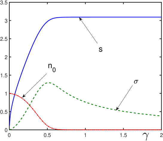
Figure 1: Condensate (quasi-condensate) fraction $n_{0}$ (dash-dotted line), anomalous average $\sigma$ (dashed line), and sound velocity $s$ (solid line) as functions of the gas parameter $\gamma$.

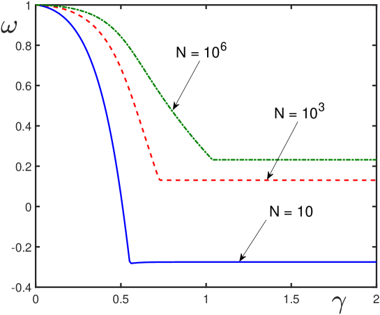
Figure 2: Order index $\omega(\hat{\rho}_{1})$ as a function of the gas parameter $\gamma$ for different numbers of trapped atoms: $N=10$ (solid line), $N=10^{3}$ (dashed line), and $N=10^{6}$ (dash-dotted line).

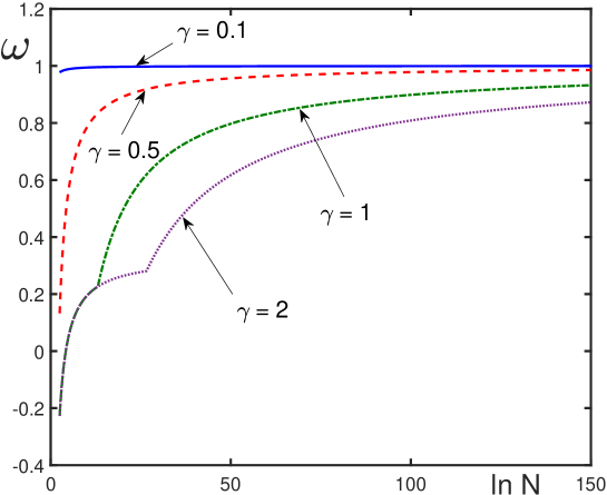
Figure 3: Order index $\omega(\hat{\rho}_{1})$ as a function of $\ln N$ for different values of the gas parameter: $\gamma=0.1$ (solid line), $\gamma=0.5$ (dashed line), $\gamma=1$ (dash-dotted line), and $\gamma=2$ (dotted line).