Neural network based path collective variables for enhanced sampling
of phase transformations

Abstract

We propose a rigorous construction of a 1D path collective variable to sample structural phase transformations in condensed matter. The path collective variable is defined in a space spanned by global collective variables that serve as classifiers derived from local structural units. A reliable identification of local structural environments is achieved by employing a neural network based classification. The 1D path collective variable is subsequently used together with enhanced sampling techniques to explore the complex migration of a phase boundary during a solid-solid phase transformation in molybdenum.

Efficient sampling of high-dimensional conformational spaces represented by rough potential energy landscapes constitutes a significant challenge in the computational molecular sciences, particularly when different basins on the landscape are separated by energy barriers significantly higher than $k_{\rm B}T$. In order to address this challenge, various enhanced sampling techniques have been developed including accelerated molecular dynamics Voter (1997, 1998); Sørensen and Voter (2000); Voter et al. (2002); Perez et al. (2009), transition path sampling Dellago et al. (1998a, b); Dellago et al. (2002); Bolhuis et al. (2002), metadynamics Laio and Parrinello (2002); Laio et al. (2005); Laio and Gervasio (2008); Barducci et al. (2008), and (driven) adiabatic free energy dynamics (d-AFED) Rosso et al. (2002); Rosso and Tuckerman (2002); Abrams and Tuckerman (2008) or temperature accelerated molecular dynamics (TAMD) Maragliano and Vanden-Eijnden (2006) and combinations of these Chen et al. (2012); Awasthi and Nair (2017). In many cases the sampling, and in essentially all cases the analysis of the resulting high-dimensional free-energy landscapes, requires a projection onto a low-dimensional collective variable (CV) space. Indeed, the choice of the CVs is not always intuitive, but a meaningful representation in the low-dimensional space is crucial for capturing the correct mechanisms.

Machine learning (ML) can provide a powerful approach to address the aforementioned challenges. The last decade has seen significant advances in the use of electronic structure calculations to train ML potentials for atomistic simulations capable of reaching large systems sizes and long time scales with accurate and reliable energies and forces. More recently, ML approaches have proved useful in learning high-dimensional free-energy surfaces (FESs) Schneider et al. (2017); Chiavazzo et al. (2017), and in providing a low-dimensional set of CVs Zhang and Chen (2018); Jung et al. (2019). In such approaches, however, it is often difficult to interpret the low-dimensional CVs that emerge from the learning procedure as they emerge as abstract outputs of the ML model employed. In this letter, we overcome this difficulty by exploiting an ML model to identify local atomic structures and then using the ML output to construct a physically motivated one-dimensional CV. The latter is then employed with an enhanced configurational sampling scheme to characterise structural phase transformations in condensed matter. The basic idea of our approach is generally applicable to tackle different kinds of phases transformations.

A structural phase transformation can be viewed as a global change of the entire system that is associated with and driven by changes in the local structural environment around each atom (or other structural building blocks such as molecules). Furthermore, for each phase of interest (different crystalline structures, liquid and amorphous phases) we can define a distinct CV that quantifies the amount of a particular phase within the system. These global CVs form an $n$-dimensional space of clasifiers where $n$ is the number of phases and any transformation between different structures can be described as a path in this classifier space. For each path we can construct a one-dimensional path collective variable Branduardi et al. (2007) as a non-linear combination of the global classifier CVs. The path CV can then be used in an enhanced sampling scheme, to project free energies, or to analyse the mechanism along the transformation. Our approach to derive the 1D path CV correspondingly involves three steps: first, we use a classification neural network (NN) Behler (2011a); Geiger and Dellago (2013) to identify the local structural environment around each atom in terms of the involved phases; next, this local information is combined into global classifier CVs, e.g. as the fraction of each structure in the system; finally, we define a path that connects two phases in the classifier space and compute the corresponding path CV.

As an illustration of our approach, we study the solid-solid transformation between the topologically close-packed (TCP) A15 and the body-centred cubic (bcc) phase in molybdenum. TCP phases are of particular interest in high-performance materials such a Ni-base superalloys Reed (2006) as their formation significantly influences the materials properties Rae and Reed (2001). In tungsten, the transformation between the A15 and bcc phase has recently attracted increased attention Liu and Barmak (2016); Barmak et al. (2017) since for applications in microelectronics the formation of A15 should be avoided Rossnagel et al. (2002); Choi et al. (2011) whereas in spintronic devices the A15 phase is the desired one Pai et al. (2012). In a previous study the dynamics of the A15-bcc phase boundary in Mo was investigated using the adaptive kinetic Monte Carlo (AKMC) approach Duncan et al. (2016). It was found that the phase boundary moves via collective displacements of groups of atoms through a disordered interface region which was associated with an effective barrier for the formation of a new bcc layer. Solid-state nudged elastic band calculations likewise indicate that the minimum energy path at $T=0$ K favors the nucleation of an interface and growth by phase boundary migration over a concerted mechanism Xiao et al. (2014). Here, we demonstrate how we can efficiently sample the phase space explored during phase boundary migration by combining the 1D path CV with d-AFED/TAMD Rosso et al. (2002); Rosso and Tuckerman (2002); Maragliano and Vanden-Eijnden (2006); Abrams and Tuckerman (2008) and metadynamics Laio and Parrinello (2002); Laio et al. (2005); Laio and Gervasio (2008); Barducci et al. (2008) and characterise the free energy landscape along the A15 to bcc phase transformation.

The first step in constructing the path CV for structural phase transformations is the identification of the local structural environment. The NN for structure classification applied in this work is based on a framework proposed by Geiger and Dellago to distinguish various polymorphs of ice Geiger and Dellago (2013). We use a feed-forward NN where the input layer is given by a set of functions for each atom that serve as structural fingerprints. Specifically, we use a mixture of a subset of the Behler-Parrinello symmetry functions, which were introduced to interpolate potential energy surfaces in condensed matter systems using NNs Behler and Parrinello (2007); Behler (2011b), and the Steinhardt bond order parameters Steinhardt et al. (1983). Both the symmetry functions and the Steinhardt parameters are invariant with respect to rotation, translation, and the exchange of two atoms of the same element. To make the structure classification using the NN efficient, the number of input functions should be kept small. In addition, the input functions should be simple and as short ranged as possible. By combining the symmetry functions with the Steinhardt parameters we were able to reduce the number of input functions to 14, with 11 symmetry functions of two different types and three Steinhardt bond order parameters with $l=6,7,8$ (details regarding the input functions are given in the Supplemental Material sup ). For comparison, 45-50 symmetry functions of four different types were used in Ref. Geiger and Dellago, 2013. Use of a smaller subset of the full set of input functions, i.e., only the symmetry functions or only the Steinhardt parameters, does not provide enough information as input to NN, thereby degrading the accuracy of the structure classification.

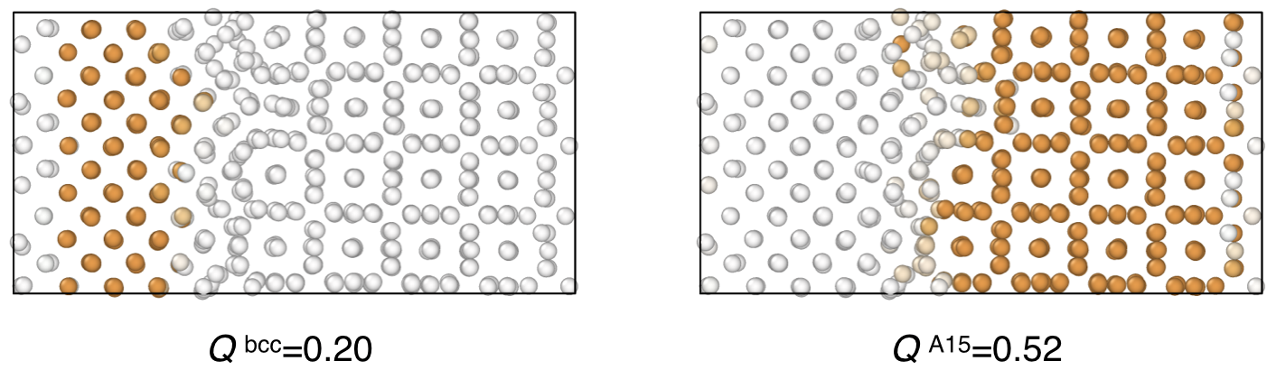
Figure 1: Initial interface setup after equilibration at $T=300$ K; atoms are coloured according to their local structural order parameter value determined using the NN for $q_{i}^{\text{bcc}}$ (left) and $q_{i}^{\text{A15}}$ (right) with a colour scheme from white ($q_{i}^{j}=0$) to orange ($q_{i}^{j}=1$). $Q^{\text{bcc}}$ and $Q^{\text{A15}}$ are the values of the global CV defined in Eq. (1).

The output of the NN is a vector $\mathbf{q}_{i}$ for each atom $i$ with one component $q_{i}^{j}$ for each of the structures $j$ of interest with $q_{i}^{j}\in[0,1]$. In the present study, this includes bcc and A15 as well as face-centred cubic (fcc), hexagonal close packed (hcp), and a disordered structure (dis). The disordered phase comprises local structural environments that significantly deviate from a well-ordered crystal phase and would be characteristic of amorphous or liquid phases. In the A15-bcc phase boundary migration, this also pertains to the disordered interface region between the two crystal bulk phases. We have used both normalised and unnormalised vectors $\mathbf{q}_{i}$, but in the present application, we did not observe any noticeable differences. The NN was trained using snapshots from molecular dynamics (MD) simulations at different temperatures and for the different phases. Additional snapshots were taken from dynamical simulations of a supercell containing atoms in the A15, bcc, and interface region. In total 346,436 local atomic environments were used to train the weights of the NN (further details are given in the Supplemental Material sup ). In Fig. 1 the initial setup of the bcc-A15 interface is shown where the atoms are coloured according to the output of the NN for $q_{i}^{\text{bcc}}$ (left) and $q_{i}^{\text{A15}}$ (right). The NN clearly identifies the two crystalline regions.

The second step in constructing the path CV consists in using the atomic output vectors of the NN to define global classifier CVs for each phase. In particular, for phase boundary migration, we define a global CV as the average over the local phase classification. For example, for bcc the global CV is

$$Q^{\text{bcc}}=\frac{1}{N}\sum_{i=1}^{N}q_{i}^{\text{bcc}}\quad,$$ (1)

where $N$ is the number of atoms in the simulation cell. Classifier CVs for the other phases, $Q^{\text{A15}}$, $Q^{\text{fcc}}$, $Q^{\text{hcp}}$, and $Q^{\text{dis}}$ are similarly obtained. Within this definition the classifier CVs describe the phase fractions for any given configuration.

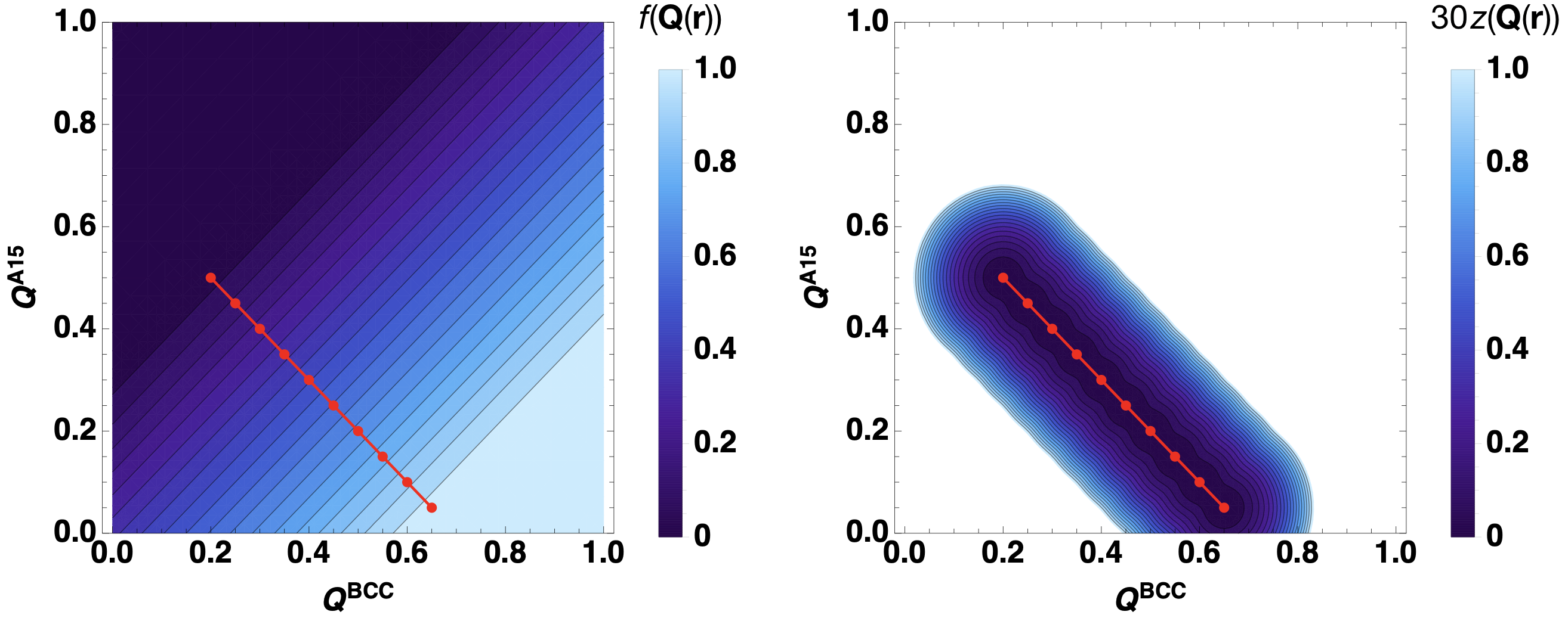
Figure 2: Left: path collective variable $f(\mathbf{Q}(\mathbf{r}))$ in the $Q^{\text{bcc}}-Q^{\text{A15}}$ space. Right: distance function $z(\mathbf{Q}(\mathbf{r}))$ (multiplied by a factor of 30) in the $Q^{\text{bcc}}-Q^{\text{A15}}$ space. The red lines indicate the path along the nodal points.

The final step consists in constructing a path CV in the space spanned by the global classifier CVs. In the case of the phase transformation between bcc and A15, we choose a path in the $Q^{\text{bcc}}-Q^{\text{A15}}$ space where the sum of the phase fractions is constant. The path CV is defined as Branduardi et al. (2007)

$$f(\mathbf{Q}(\mathbf{r}))=\frac{1}{P-1}\frac{\sum_{k=1}^{P}(k-1)\exp(-\lambda|\mathbf{Q}(\mathbf{r})-{\bm{Q}}_{k}|^{2}|}{\sum_{k=1}^{P}\exp(-\lambda|\mathbf{Q}(\mathbf{r})-{\bm{Q}}_{k}|^{2})}\quad,$$ (2)

where $\mathbf{Q}(\mathbf{r})=\{Q^{\text{bcc}},Q^{\text{A15}}\}$ is the position in the $Q^{\text{bcc}}-Q^{\text{A15}}$ space, ${\bm{Q}}_{k}$, $k=1,...,P$ are the $P$ nodal points along the path, and $|\mathbf{Q}(\mathbf{r})-{\bm{Q}}_{k}|^{2}$ is the square distance from the path in classifier space. The path has $P=10$ equidistant points and follows the diagonal from ${\bm{Q}}_{1}=\{0.2,0.5\}$ to $\bm{Q}_{10}=\{0.65,0.05\}$. In order to provide a meaningful representation of the path CV in its discretised form in Eq. (2), $\lambda$ should approximately be set to the inverse of the square distance between consecutive nodal points, yielding $\lambda=200$. The value of the path CV together with the path in the $Q^{\text{bcc}}-Q^{\text{A15}}$ space is shown in the left graph of Fig. 2. It smoothly increases from 0 to 1 as the path fraction of bcc increases and the one of A15 decreases. Perpendicular to the path the value of the path CV is constant. In addition, the function Branduardi et al. (2007)

$$z(\mathbf{Q}(\mathbf{r}))=-\frac{1}{\lambda}\ln\left(\sum_{k=1}^{P}\exp(-\lambda(\mathbf{Q}(\mathbf{r})-{\bm{Q}}_{k})^{2})\right)$$ (3)

can be used as a distance measure from the path. $z(\mathbf{Q}(\mathbf{r}))$ can either be used as additional biasing coordinate or as a restraining potential Cuendet et al. (2018). In the right graph of Fig. 2 $z(\mathbf{Q}(\mathbf{r}))$ (multiplied by a factor of 30) is shown for $\lambda=1000$ com .

The path CV defined in Eq. (2) is subsequently employed in d-AFED/TAMD simulations to enhance the sampling of the bcc-A15 phase transformation. In d-AFED Abrams and Tuckerman (2008), specifically, the physical system is coupled to an extended variable $s$ through a harmonic potential where the Hamiltonian in the extended phase space with a single variable $s$ and conjugate momentum $p_{s}$ is given by

$$\tilde{H}(\mathbf{r},\mathbf{p},s,p_{s})=H(\mathbf{r},\mathbf{p})+\frac{p_{s}^{2}}{2\mu_{s}}+\frac{1}{2}\kappa(f(\mathbf{Q}(\mathbf{r}))-s)^{2}\quad.$$ (4)

Here, $H(\mathbf{r},\mathbf{p})$ is the Hamiltonian of the unperturbed system, $\mu_{s}$ is the “mass” of the extended variable, $\kappa$ is the harmonic coupling constant, and $f(\mathbf{Q}(\mathbf{r}))$ is the corresponding path CV in Eq. (2). In order to ensure that the free energy profile $F(s)$ along the extended variable is correctly generated, an adiabatic decoupling between the physical and extended variables is needed Abrams and Tuckerman (2008) and is achieved by choosing a large value of the mass parameter $\mu_{s}$. In this adiabatic limit, the sampling is accelerated by running the dynamics of the extended variable $s$ at a high temperature $T_{s}\gg T$.

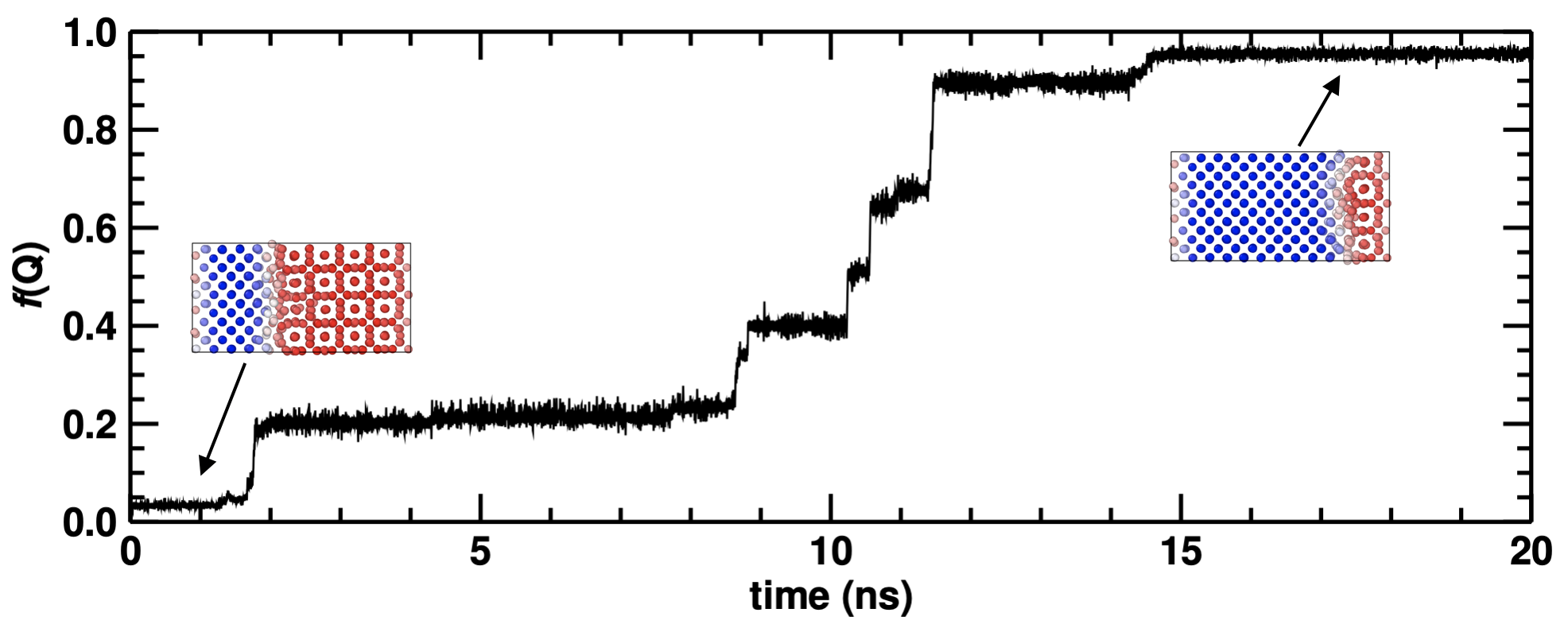
Figure 3: Path collective variable $f(\mathbf{Q}(\mathbf{r}))$ as a function of time during a d-AFED run. As the bcc phase grows the path CV increases from 0 to 1. Blue atoms are in a bcc, red atoms in an A15 environment.

In Fig. 3 the evolution of the path CV is shown for a representative d-AFED run in the NVT ensemble with a system temperature of $T=300$ K, an extended variable temperature of $T_{s}=3000$ K, $\mu_{s}/\bar{\mu}_{\text{eff}}\approx 1000$ (where $\bar{\mu}_{\text{eff}}$ is the average effective mass of the path CV Cuendet and Tuckerman (2014)), and $\kappa=2\times 10^{5}$ eV (further details are given in the Supplemental Material sup ). The entire A15 phase is transformed into bcc in less than 20 ns whereas in the unbiased system the transformation usually takes tens of microseconds Duncan et al. (2016), emphasising the significant speed-up in the exploration of the phase space achieved by d-AFED. From the simulations we can estimate the free energy along the extended variable, $F(s)$, from the mean force on $s$ due to the coupling to the physical system

$$\frac{\partial F(s)}{\partial s}=-\langle\kappa(f(\mathbf{Q}(\mathbf{r}))-s)\rangle_{s}^{\text{adb}}\quad.$$ (5)

The free energy profile for the A15 to bcc transformation extracted from 50 d-AFED runs is shown in the top graph of Fig. 4.

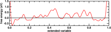
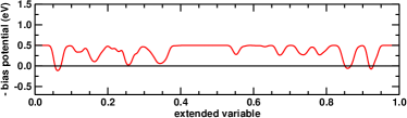
Figure 4: Top: free energy profile along the extended variable $s$ at $T=300$ K extracted from the potential of mean force of the d-AFED simulations with $T_{s}=3000$ K. Bottom: negative of the bias potential from the metadynamics simulations.

The profile does not correspond the equilibrium free energy surface but rather reflects the one-way transition from A15 to bcc. An observation of the reverse transition is not possible within this simulation cell due to the large interface mismatch between bcc and A15 (-6.73%) and corresponding large energy difference as well the overall large pressure in the small simulation cell ($\approx 200$ kbar). This particular system setup was chosen as a test case to compare our approach to previous results, where an effective barrier of $\Delta E_{\text{layer}}=0.47\pm 0.07$ eV for the formation of a bcc layer was extracted from AKMC simulations Duncan et al. (2016). The free energy profile in Fig. 4 clearly reflects the layer-by-layer transition observed in this system, and the respective energy barriers are $\approx 0.5$ eV, which is comparable to the effective barrier in Ref. Duncan et al., 2016. Deviations for small and large values of $s$ are expected since at small values the interface needs to equilibrate from its initial configuration, and at large values, interactions with the second, fixed interface in the simulation cell become more pronounced. Overall the agreement with previous results is very good.

In order to test the robustness of our 1D path CV, we have also used it in metadynamics simulations. In metadynamics Laio and Parrinello (2002); Laio and Gervasio (2008) a time-dependent bias potential as a function of the CV is added to the Hamiltonian, usually in terms of Gaussians, that accelerates the exploration of the phase space by gradually filling up the wells of the energy minima. When all minima are filled, the corresponding free energy surface becomes flat and the system exhibits a diffusive behaviour along the CV. The inverse of the bias potential can be used as an estimator for the free energy. In our metadynamics simulations, we again do not converge to the equilibrium free energy surface but only obtain a rough first estimate for the one-way transition from A15 to bcc. A representative free energy profile $F(s)=-V^{\text{bias}}(s)$ is shown in the bottom graph of Fig. 4 (details concerning the metadynamics simulations are given in the Supplemental Material sup ). The shape again clearly indicates a layer-by-layer transition and the corresponding energy barriers are close to the expected value of 0.5 eV. Since the formation times for a new bcc layer follow an exponential distribution typical of a rare event, the gradual filling of energy minima in the metadynamics simulation in only one direction will correspondingly result in a range of barriers including even some flat parts along the path CV. In the d-AFED simulations we can average the mean force in Eq. (5) over multiple runs where each run contributes to an extensive sampling of all degrees of freedom perpendicular to $s$.

In a less constrained system, where the reverse phase transformation is also possible, we can explore both the forward and backward transition along the 1D path CV. As an example, we have chosen the same system as above, but the simulations are now performed at constant (zero) pressure. In addition to the bias potential from the metadynamics simulations, we apply a restraining potential on the distance from the path CV $z(\mathbf{Q})$ in Eq. (3) with $V^{\text{rest}}(z)=k((z-z_{0})/\epsilon)^{2}$, where $z_{0}=0.0$, $k=30$ eV, and $\epsilon=0.05$.

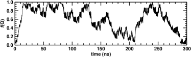
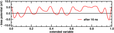
Figure 5: Top: evolution of the path CV $f(\mathbf{Q}(\mathbf{r}))$ during the NPT metadynamics simulation at $T=300$ K. Middle: negative of the bias potential after 16 ns. Bottom: negative of the bias potential after 16 and 290 ns.

The evolution of the path CV during the simulation is shown in the top graph of Fig. 5. Up to about 16 ns the path CV increases monotonically to its maximum value indicating the first, complete A15 to bcc transformation. The corresponding energy profile (negative of the bias potential) is depicted in the middle graph of Fig. 5, again exhibiting the characteristic shape of a layer-by-layer transformation. The energy barriers are much larger ($\approx 5$ eV) than in the previous case, which can be attributed to a decreased driving force (as qualified by the potential energy difference between the two phases) and interface mobility at constant $P=0$, as well as to the additional restraining potential. As the bias potential continues to build up, the system starts to show a diffusive behaviour along the path CV. Between $210-290$ ns the system transforms smoothly from A15 to bcc and back to A15. Observing this behaviour was only possible when employing the unique 1D path CV suggested here. Although we did not carry out constant-pressure d-AFED simulations, we expect the same behavior would be obtained Yu et al. (2014). In developing this new approach, we initially investigated several other 1D CVs, and we also tried to sample the 2D CV space of phase fractions directly, but none of these simulations achieved a full sampling of the forward and backward phase transformations. The free energy profile after 290 ns is shown in the bottom graph of Fig. 5. Clearly, the bcc phase is much lower in energy within this particular supercell setup and the barrier for the transformation from bcc to A15 is a factor of four larger than for the A15 to bcc transition. This is consistent with our unbiased MD simulations, where even for very high temperatures, the reverse transition was never observed. For a quantitative analysis of the interface migration barriers, simulations cells with a smaller mismatch and a larger interface area will be considered in future studies.

In summary, we have proposed a general approach how to rigorously construct a 1D path CV for sampling phase transformations. The method is based on a local structure classification using a neural network and this local information is then combined into global classifier CVs for each phase of interest. Finally, the phase transformation can be described as a path in the $n$-dimensional classifier space and the corresponding 1D path CV can be computed as a non-linear combination of the global classifier CVs. We have shown the applicability of our approach to the solid-solid phase transformation between the bcc and A15 phases, which proceeds via phase boundary migration characterised by complex atomic rearrangements at the interface. Combining the 1D path CV with enhanced sampling techniques, we were able to estimate the energy profile along the transformation and, for the first time, simulate the growth of the A15 phase from the bcc phase. Due to the computational efficiency in exploring the phase space, our approach enables the study of phase transformations in much larger simulation cells where it will be possible to consider realistic interface mismatches and transformation mechanisms including the formation of a step and growth along the step edges.