A Comparison of the Chemical Composition of Main Sequence and
Giant Stars in the Open Cluster NCC 752

Abstract

The chemical composition of stars in open clusters provides the best information on the chemical evolution of stars via comparison of the main sequence stars with the evolved giants. This is a case study of the abundances in the dwarfs and giants in the old, open cluster, NGC 752. It is also a pilot program for automated abundance determinations, including equivalent width measurements, stellar parameter determinations, and abundance analysis. We have found abundances of 31 element-ion combinations in 23 dwarfs and 6 giants. The mean cluster abundance of Fe is solar with [Fe/H]$=-0.01\pm 0.06$ with no significant difference between the dwarfs and giants. We find that the cluster abundances of other elements, including alpha-elements, to be at, or slightly above solar levels. We find some evidence for CNO processing in the spectra of the giants. The enhancement of Na in giants indicates that the NeNa cycle has occurred. The abundances of Mg and Al are similar in the dwarfs and giants indicating that the hotter MgAl cycle has not occurred. We find no evidence of s-process enhancements in the abundances of heavy elements in the giants.

1 Introduction

Cluster stars, with their common origin and shared evolutionary environment, provide laboratories for analyzing atmospheric processes and for exploring compositional variances between stars with differing initial masses. Studies of cluster stars are able to utilize a large, homogeneous sample to represent a cross-section of the stellar population of a given age and origin. A cluster represents conditions at a given time and galactic location. Therefore, comparative studies between cluster member stars have distinct advantages over single star or randomly selected field star studies.

Prior cluster studies have leveraged the material and temporal common origin of cluster stars to establish trends with various cluster characteristics. Sample previous studies have examined the relationship between metallicity and age (e.g. Phelps, Janes & Montgomery 1994), or metallicity, age, and galactic location (e.g. Friel et al.  2002). Other cluster studies have produced or supplemented catalogs of elemental abundances for large numbers of elements, stars and clusters (e.g: Pancino et al.  2010). The aforementioned cluster studies take advantage of the common origin assumption, and determine cluster abundances and metallicity measurements from small numbers of either giant or dwarf stars.

The primary goal of this study is to provide a comprehensive elemental abundance analysis of the stars in NGC 752. We have included both giant and dwarf stars in our sample. With the exception of some light elements (Li, Be, and B, q.v.:Boesgaard et al.  (2016)), we can assume that the atmospheric elemental abundances, as measured in our dwarf sample are representative of the unaltered stellar nebula from which they formed. We then compare the abundances as measured in our giant sample, which have undergone a “dredge-up” of core material into their atmospheres, to those from our dwarf sample. We evaluate the differences to gain insights into the core nuclear processes which have occurred over the main-sequence lifetime of the stars.

Within the past decade, large, easily accessible, digitally archived spectral data have become widely available. These public archives provide an opportunity to analyze data and publish discoveries, without the necessity of exclusive telescope time. Our observational data has been drawn exclusively from publicly available archive data. As our chosen spectra have been taken by mutiple investigators, with different science goals, our resulting data set has a wide variance in wavelength coverage and signal-to-noise.

A second goal of this study is to establish methods for automated cluster abundance evaluation, using previously collected, archived spectral data. By using a rudimentary artificial intelligence, we implemented an objective measurement algorithm which removed several repetitive, error-prone, or subjective processes from the abundance and stellar parameter determinations.

For this study, we selected data from the HIRES spectrograph (Vogt et al.  1994) on the 10m W.M.Keck I telescope. We also use a solar reference spectrum from the National Solar Observatory (Wallace et al.  2011), and solar calibration spectra from the ESO’s HARPS (Mayor et al.  2003) instrument.

We measured the abundances of a comprehensive list of 25 elements, 6 in both singly-ionized and neutral states, across the 23 dwarfs and 6 giants. Our abundance measurements were determined through spectral synthesis and equivalent width measurements of absorption features drawn from a list of approximately 2700 lines. While our chosen spectra contain observations spanning from the near-UV (3360 Å) to the near-IR (9140 Å), we restrict our evaluation to the (mostly-) optical range ranging from 4500 Å to 8500 Å.

2 NGC 752

We have selected NGC 752 as the first cluster in our study due to a number of factors. It is a member a relatively small number of “solar twin” clusters, having a metallicity approximately solar ([Fe/H]$=+0.04\pm 0.01$ Blanco-Cuaresma et al.  (2014), [Fe/H]$=-0.063\pm 0.013$ Maderak et al.  (2013), [Fe/H]$=+0.08\pm 0.04$ Carrera & Pancino (2011)). For calibration purposes, using near-solar metallicity targets permits us to use the Sun as a reference spectrum to confirm laboratory-determined absorption line parameters with observational measurements. NGC 752 is relatively old open cluster, with an age between 1.5 and 1.8 Gyr (1.45 Gyr Anthony-Twarog et al.  (2009),  1.6 Gyr Carrera & Pancino (2011), 1.78 Gyr Daniel et al.  (1994)). NGC 752 shows evidence of either dynamic or tidal dispersal particularly in the lower main-sequence (Carraro, Monaco & Villanova 2014). While we do not utilize spectra from the late-K and M region affected by this dispersal, the loss of these lower mass stars is possible evidence that NGC 752 is well into the process of disappearing into the galactic field.

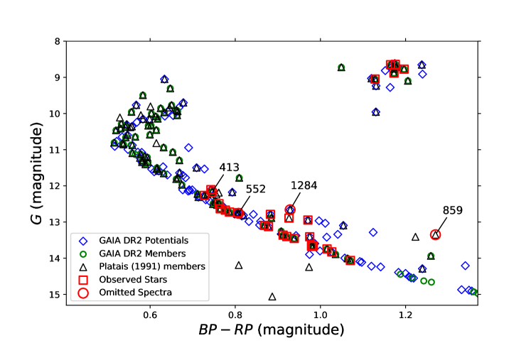
Figure 1: The color-color digagram for NGC 752. Photometry from GAIA’s Data Release 2 (DR2) (Gaia Collaboration et al.  2018). Target stars for this work are designated by red squares; stars designated as cluster members by Platais (1991) are black triangles, potential and probable additional members, as determined from the GAIA DR2 dataset (Lum 2019, in prep), are designated by blue diamonds and green circles, respectively. We also note the locations of the four Platais member spectra which we do not include in our analysis. Stars which are listed as both members in Platais, and which we consider (potential) members from the GAIA photometry/astrometry, have both the black triangle, and the appropriate GAIA marking.

Figure 1 places each of our target stars on a color-color diagram, based on photometry from the GAIA “Data Release 2” (DR2) (Gaia Collaboration et al.  2018). Also noted on the figure are the stars denoted as members by Platais (1991). We have also included stars from the GAIA dataset which appear to be members, based on analysis of position, proper motion, and parallax from DR2 (Lum 2019, in prep).

At NGC 752’s age, the main-sequence turn off stars are F-type stars. These stars lie on the blue side of the Li “gap” (Boesgaard & Tripicco 1986), implying that sufficient mixing occurs during the main sequence lifetime of the star to have carried surface material to a depth where Li can be destroyed by (p,$\alpha$) reactions. Hobbs & Pilachowski documented both the Li destruction in NGC 752 giants (Pilachowski, Saha & Hobbs 1988) and the presence of the “Li gap” in the F-stars (Hobbs & Pilachowski 1986; Pilachowski & Hobbs 1988). Deep mixing mechanisms may also affect atmospheric elemental abundances, as measured at the surface, after the first dredge up portion of the red giant branch.

We selected 29 stars, 23 dwarfs and 6 giants, within the cluster to perform a complete, precise accounting of the material composition of the cluster. We analyzed differences between the evolved and unevolved members, with the aim of quantifying the compositional changes between the evolutionary stages of our sample sets. Our sample spectra uses archived observational data from the Keck Observatory Archive (KOA).

3 Stellar Spectra Data

3.1 NGC 752 spectra from Keck HIRES

Table LABEL:tab:752Obs lists the J2000 coordinates (RA/Dec), spectral wavelength range, and the signal-to-noise for the composite spectra of each star in our survey. We chose the Platais (1991) identifiers for our reference, but have included cross-references for Heinemann (1926) and Rohlfs & Vanysek (1962) (WebDA) as reported by the SIMBAD astronomical database (Wenger et al.  2000). The wavelength ranges cited reflect the minimum and maximum values for each spectrum. The spectral coverage for a given range is generally not complete, due to inter-order gaps and gaps between coverage of individual observation configurations.

All NGC 752 spectra were obtained from the Keck Observatory Archive (KOA) and were measured using the HIRES spectrograph, with a resolution of ~48,000, as calculated from the instrument setup parameters (KOA “SPECRES” keyword). We utilize observations from both the “original” (prior to August 2004) and “upgraded” (post-2004) HIRES. The upgraded detector added two CCDs, for a total of three, increasing the wavelength coverage while reducing pixel size from $24\mu$ to $15\mu$ .The difference between the two detectors is significant, and manifests in our data as a difference in the signal-to-noise ratio with respect to exposure time, and increase in wavelength coverage for a given spectrum.

Table LABEL:tab:752Obs lists the signal-to-noise (S/N) ratio at the specified wavelength; there are one or two measurements, depending on the wavelength coverage of the spectrum. The reported S/N values are an average, rounded to the nearest ten, for the region as reported by the MAKEE (Barlow 2008) software, during the reduction process. For the representative measures, we selected two regions, the first near 6200 Å, the region containing the $T_{eff}$ calibration lines, and the second near 7800 Å, where we measured the O I triplet.

Our minimum measured S/N ratios of 40-60 for the dwarf sample are similar to those of comparable studies - eg: Maderak et al.  (2013) had a minimum S/N of 60. The S/N ratio of the giant star spectra in this study are significantly higher than those of other studies, topping out at well over 400. The S/N range in the Böcek Topcu et al.  (2015) giant study was 140-290, while Reddy, Giridhar & Lambert (2012) had S/N ratios in the 100-120 range.

We opted to use the spectra as reduced by the KOA process, heeding the warning that “the quality and content of the data…may not necessarily be suitable for publishable science.” (https://koa.ipac.caltech.edu/UserGuide/HIRES/extracted.html). Our reasoning being that, should we choose to do our own reduction, we would use the same tools- specifically MAKEE, choice of calibration frames (as suggested by the archive search), and process as the automated pipeline. We do not have sufficient knowledge of the observation session to override the recommendations of the archive. However, we performed several calibration processes in addition to the archive calibrations. We applied wavelength correction to the pipeline’s wavelength solution, using a selection of Fraunhofer and other strong iron lines. We also normalized each spectrum to a continuum level of 1.0, using a $5^{th}$ order polynomial fit for each spectral order, which we found as the highest-order polynomial we could use to fit the relatively smooth regions of the longer wavelength orders of the spectra, without over-smoothing the broad lines, and “noisier” regions. In the cases where multiple spectra were available for a single star, we co-added each spectrum using a weighted mean, using the STScI’s IRAF function scombine, with each weighted by its signal-to-noise ratio.

As a final spectra quality control process, we performed a visual inspection of the individual orders, as provided in the Keck Observatory Archives image previews. We excluded two orders (out of several hundred) which showed evidence of reduction or observational faults. In both cases, the missing orders were conveniently duplicated in other spectra, without the flaws.

During our analysis process, we elected to exclude spectra for four stars from our final results. Although high resolution and high S/N spectra were available for PLA-413, PLA-552, PLA-859, and PLA-1284, they were excluded for the following reasons: For PLA-859, the parallax data from GAIA DR2 ($0.28\pm 0.04$mas) places it beyond the cluster (mean parallax from GAIA DR2 data of $2.2\pm 0.1$, Lum (2019, in prep)). For PLA-1284, our automated process for measuring absorption lines in this (SB2) binary system did not properly account for the shifted components. After analysis, we found that the spectroscopic binary, PLA-552 displayed evidence of line broadening, which affected abundance calculations (particularly of Ti and Cr). While PLA-413 is not catalogued as a spectroscopic binary, it lies above NGC 752’s main sequence, near other binaries, and displays identical broadened metal lines. For this reason, we have also excluded both PLA-552 and PLA-413 from our final analysis.

3.2 Data Processing

Due to the relatively large number of spectra (47) and large number of lines to measure ($\sim 2700$ per spectrum), we created a series of automated processes for analyzing our spectra. The code consists of mostly Python scripts, with some calls to external C and Fortran functions. Intermediate data products, such as spectral line physical parameters (e.g. log $g_{f}$, excitation potential), equivalent width measurements, spectra file data, “astrophysical” log$g_{f}$ corrections, etc. are stored in a SQLite3 database. The code is freely available on github at: https://github.com/mikelum/ClusterAnalysis.

Our software is responsible for: a) management of the line list database and associated references, b) absorption line measurement and equivalent width calculation, c) stellar atmosphere parameter determination, and d) elemental abundance determination. It also produces plots and tables used in data analysis and in this work. In addition, we used (Stetson & Pancino 2008, DAOSpec) software routines to assist with and calibrate our Doppler corrections. We also used IRAF and STDAS (Space Telescope Science Institute 2014) for spectra stacking and continuum normalization. Our elemental abundance calculations were obtained through use of MOOG (Sneden 1973; Sneden et al.  2012) synth, blends, and abfind “drivers”. Our analysis spanned several MOOG version upgrades, between 2014 and 2017. We see no significant difference in results between the earliest (July 2014) and latest (February 2017) versions. Note that we have made superficial and cosmetic modifications to the standard MOOG program and make files to allow compilation under the GNU Compiler Collection’s GFortran (Free Software Foundation, https://gcc.gnu.org/) compiler, and removed status messages to allow the MOOGSILENT function to run truly silently.

As mentioned previously, our spectra cover a wide range of S/N ratios and resolutions from two different versions of the HIRES instrument. We account for lower resolution and/or lower S/N ratios by establishing a minimum EQuivalent Width measurement (EQW) for any given spectra of five (5) times the product of the resolution (in mÅ/pixel) and inverse of the signal-to-noise, with a minimum of 2.0 mÅ. The calculated minimum EQW limit for each star is listed in Table LABEL:tab:atmParms (see additional discussion of Table LABEL:tab:atmParms in section 3.3). Similarly, with lower S/N ratios, we expect higher uncertanties and lower sensitivity to weaker absorption lines. Figure 2 shows the region near 6200 Å which contains several Fe I lines. Temperature effects on the Fe lines are evident, and we have used them to assist with parameter determination. Over the 300K range of the three spectra in the figure, the Fe absorption lines strengthen noticeably between the hottest and coolest spectra. Figure 3 compares the Oxygen “triplet” region between 7770 and 7782 Å for three dwarf spectra with S/N of approximately 140. At this high S/N, the triplet is clearly visible, with temperature effects visible to a discerning eye as broader line widths and increased absorption in the line wings.

In addition to setting a minimum EQW measurement threshold, we also compensate for low S/N by measuring a larger sample of absorption features, where available. As an example, our list of potential Fe I lines contains over 400 entries. Our complete line list is available as an online database, with a sample format shown in Table LABEL:tab:LineList.

We include one additional criterium for accepting a measured line from lower S/N spectra. We measure the line profile in terms of the ratio of the Full Width at Half Maximum (FWHM) of the Gaussian portion of the line core (see section 3.5, below) to the resultant EQW measurement ($FWHM/EQW$). When our automated measurement process finds a potential absorption line, which was incorrectly measured from random noise fluctuation in the spectrum, the $FWHM/EQW$ ratio is almost always below 1.0 ($>99.8$% for the lowest S/N spectra). We determined this ratio limit of 1.0 through Monte Carlo (MC) measurement simulations on 250 random noise spectra. Each noise spectrum point consists of a (normalized) flux value, generated around a continuum value of 1.0, with a variance determined by the S/N being modeled. We then insert randomly selected regions from our actual data, containing a single absorption feature, into the random noise spectra. We run each noise spectrum through our line measurement process, and evaluate the resulting line measures. We apply the same criteria for line acceptability (within the linear portion of the curve of growth, within the expected wavelength range, and above the detection threshold) to these line candidates, eliminating approximately 80% of the (false) lines from a noise spectrum prior to applying the line profile criterium. We are able to recover 100% of “real” lines inserted into our test spectra, using the 1.0 (FWHM/EQW) ratio limit, and incorrectly classify less than 0.2% of the “false” lines as legitimate measurements. Of the incorrectly measured lines, an average of 3 per Monte Carlo run of 2700 lines in 250 simulated spectra passed both the 1.0 ratio limit and the line acceptability criteria, as listed above.

3.3 Absorption Line Evaluation

One of our goals of this project was to produce a method for selecting target lines, using objective criteria, from all available measured transitions within our spectral coverage range. Most comparable abundance studies will use a substantially smaller set of “trusted” lines, adopted from previous, similar studies, and/or lines which have been reliable for the particular researcher in their prior work. In our own work (e.g. Boesgaard, Lum & Deliyannis (2015); Boesgaard, Roper & Lum (2013)), we have opted for a combination of the two selection processes.

For small-scale, high-resolution, high S/N studies, this process works well. However, for larger-scale and potentially lower S/N studies, a much larger sample of lines are needed. When compiling all the available line resources, including large online databases such as those run by VALD (Ryabchikova et al.  2015), and NIST (Kramida et al.  2014), we can easily find a massive number of available lines. The challenge is identifying which to use.

For this project, we categorized each of the lines in our database by measuring the line in a high-resolution solar spectrum (Wallace et al.  2011), calculating the abundance of the respective element from that line width, and then comparing the result to the calculated solar abundances from Table 1 in Asplund et al.  (2009). We then categorized the lines as “excellent”, where the difference ($\Delta$) in calculated abundance from that in Asplund et al.  is less than 0.05 dex, “good” ($0.05\leq\Delta\leq 0.10$), “fair” ($0.10\leq\Delta\leq 0.20$), “poor” ($0.20\leq\Delta\leq 0.40$), “bad/mis-measured” ($0.40\leq\Delta\leq 1.00$), and “detected” ($\Delta\geq 1.00$). We assign each of these categories a numerical “Quality” score of 10 (“excellent”), 8, 6, 4, 2, or 1 (“detected”), and also use a score of 0 for lines which were either not detected in the solar spectrum, or which were measured using spectral synthesis.

Table LABEL:tab:SolarAbs shows abundances as calculated using each of the five above categories, plus the abundance as calculated using all measured lines. Using these calculations, we determined that our line choices for Pr II and Y I were not accurate enough to use for further analysis. Similarly, we were unable to measure the small number of S I and Eu II lines in our spectral sample to provide analysis of these elements.

Our choice to base our astrophysical log $g_{f}$ values on the solar spectrum is a reasonable assumption due to the metallicity of our sample stars falling into that of solar ([Fe/H]_NGC752~+0.00). Furthermore, the atmospheric parameters for our dwarf sample is similar to solar (F,G, and K-stars). For future work in stars and clusters with metallicities and atmospheric parameters farther from solar, we will not have independently verifiable abundance values (as we do from meteoric and solar samples). For these future astrophysical log $g_{f}$ values, we expect that proper calibration of a given line’s correction requiring an iterative, statistical process. The first-order correction being the (constant) solar correction we use in this work. Future corrections would be calculated using a function of atmospheric parameters and metallicities from the abundances of a small sample of stars (such as in this work). The resulting function would be expanded through the inclusion of data from stars with increasing variance in parameters and metallicities. The eventual goal being a functional solution for the astrophysical log $g_{f}$ of any given line, based on a large sample of stellar parameters and metallicities. However, examining such a project is well beyond the scope of this work.

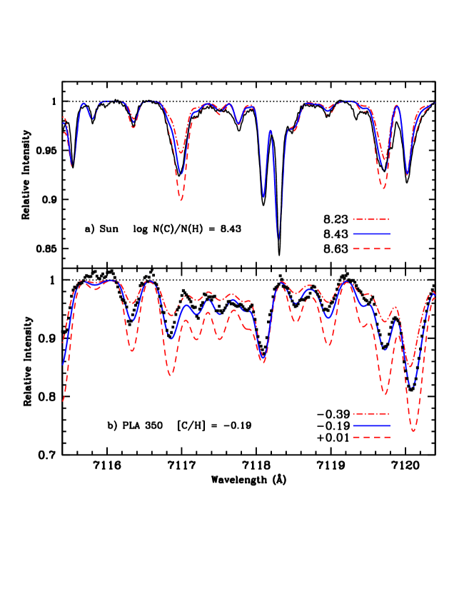
Figure 5: Comparison between the synthesis of a portion of the region used to measure C I. Note the CN molecular features between 7117 and 7118 Å are visible in the giant, PLA-350 (bottom) spectrum, but not apparent in the dwarf (solar) spectrum.

Within the wavelength range of our study, the absorption lines for both C and N are weak or are blended with other nearby lines. While our automated line measurement process can evaluate blended lines of comparable strength, we chose to supplement our C and N abundance measures with additional measurements from synthesized spectra. We used MOOG’s synth driver and line lists which combined elemental data from the VALD (Ryabchikova et al.  2015) database, with CN molecular data from Sneden et al.  (2014). We discuss the specific regions in Section 4.2. Figure 5 shows a sample synthesis of the region near 7115 Å for the Sun and for PLA-350, a red giant in NGC-752. We used this region to determine C I abundance.

3.4 Absorption Line Selection

When we measured abundances of elements with large numbers of lines in a particular spectrum, we have the option of using a subset of the lines. While the immediate tendency might be to only use the lines with the highest quality scores (as described above in Section 3.3), we must also consider the effect of adding more samples to a given population in increasing the accuracy of a measurement. In general, adding more measurements of equal quality will result in a more accurate measurement of a given quantity. However, since we know the quality of our population, our process would begin by selecting lines of the highest quality, and subsequent additions to our measurement subset would be of lower quality. For many elements, we have a relatively large number of quality-rated lines, and feel the need to address the question of accuracy vs. precision.

By hand-selecting a small number of lines, we can guarantee a precise result - simply put, we can select for small error bars. Conversely, a set of lines exists which would provide the most accurate measurement of the abundance of a given element in a given star. Unfortunately, we cannot know the latter set, without knowing the actual abundance(s) from another independant measure. For our purposes, we are interested in the most accurate measurement of atmospheric abundances. However, we also wish to have at least a “reasonable” level of precision. To answer the question of accuracy vs. precision, we created a Monte-Carlo simulation of the line measurement process.

Our simulation began with an assumption of an “actual” elemental abundance of $[X/Fe]=0.00$. We randomly generated a set of between 1 and 250 lines, distributed among the 6 “quality” categories as indicated by the population in our solar measurements (Table LABEL:tab:SolarAbs) - Approximately 16% in the top (“10”) category, 13% in the next (“8”), and 20%, 21%, 18%, and 12% in the remaining four categories, respectively. For each line, we generated an experimental abundance measurement, using a randomized Gaussian distribution around the solar value. The standard deviation ($\sigma$) used was the average $\sigma$ of all the lines in the corresponding category in our solar measurements, added in quadriture with an atmospheric term of 0.10, representative of a typical atmospheric parameter error term (see Table LABEL:tab:atmErrs). By comparing the experimental abundance, calculated as the mean of all lines of a given quality or better, with the actual value of 0.00, we determined the quality-number relationship used herein.

Our simulation ran 10,000 trials, using N=1, 3, 5, 10, 20, 50, 100, and 250 lines to measure the simulated abundance of our simulated element. We then evaluated both the accuracy and precision of abundances calculated from lines of varying “quality” ratings. Unsurprisingly, the most precise abundances were calculated when only the lines of the highest available quality ranking were used. However, as the number of available lines for a given element increase, we found that including more lines of lower quality does increase the accuracy of the measurement.

In summary, our simulation found, for elements where we measure 4 or fewer lines, using only the lines in the highest available quality category provided the most accurate abundance measurement. For example, if we measured 3 lines with quality scores of 10, 8, and 6, we would calculate the abundance, using only the single line of the highest quality (10). Should none of the measured lines for a given element have the highest quality rating, we would take the abundance as measured by lines in the next lower category, reducing our acceptable quality category until at least one line was used.

In the case where we measured between 5 and 10 lines for an element, we would not discriminate between lines of the highest two categories (10, 8), and would use all available lines in these two quality categories. As in the cases with small numbers of lines, should none of our measured lines rank in the top two quality categories, we calculated the elemental abundance using the highest quality lines available from the measured set.

For $N\geq 20$, the most accurate abundace values are achieved by using all measured lines in the top 3 categories. In all spectra for this project, when 20 or more lines were measured for a given element, a large fraction (generally the majority) of lines fell within the top three quality categories. Therefore the abundances calculated for large-N elements always used the “best” lines.

Finally, we note that for any given line, we apply the $\Delta$ value (from the solar calculation, Table LABEL:tab:SolarAbs) to our resulting abundance calculation, commonly referred to as an “Astrophysical log $g_{f}$ correction”.

3.5 Equivalent Width Measurements

Using our continuum-fit and Doppler-corrected spectra, we measured approximately 2400 absorption line features per spectrum from a list of 31 elements, 8 of which had two ionization states. We were able to obtain usable line measurements for 24 elements (7 with both neutral and singly-ionized states). A complete list of our line list (2430 lines), reference list (68) and equivalent width measurements (17000+ measurements) for all stars are available as supplemental online data.

Needless to say, with such a massive line list and large collection of spectra, we did not perform the EQW measurements manually. We utilized a combination of Python scripts and AstroPy (Astropy Collaboration et al.  2013) functions to obtain our EQW measurements (using a simple linear combination of Lorenzian and Gaussian curves). However, we found that, after trying multiple line profiles (pure Gaussian, Voight, and rudimentary linear and trapezoidal interpolations), our chosen line profile had less effect on the calculation of the equivalent width of a given line than individual data point errors from signal-to-noise, and spectral dispersion.

Our line profiles, and the resulting EQW values, are based from a localized continuum, using the values of the local maxima in the 2Å window containing the center of our target line. This process is similar to that used in Ramírez & Allende Prieto (2011), except instead of a visual inspection of the local window, our process automates the continuum placement by adding a small factor (0.02 on a 1.0-normalized continuum) to the mean of the highest local maxima. However, as with the specific form of the line fit, above, the exact placement of the local continuum has a very small effect (~1mÅ) as per Carrera & Pancino (2011).

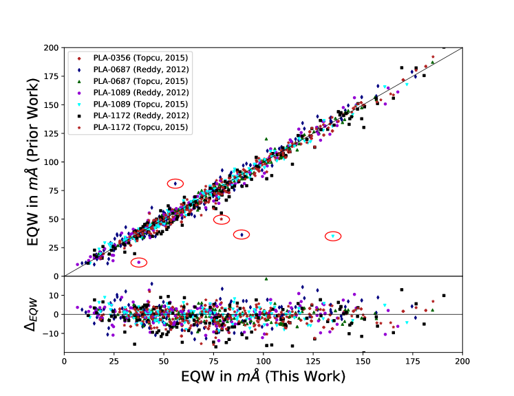
Figure 6: Comparison of 1211 Equivalent Width (EQW) measurements between Reddy, Giridhar & Lambert (2012), Böcek Topcu et al.  (2015), and this work for common giant stars. The circled outliers are discussed in the text.

Figure 6 compares the resulting equivalent width measurements taken by our automated process against over 1200 IRAF splot measurements taken by Reddy, Giridhar & Lambert (2012) and Böcek Topcu et al.  (2015). We find no systematic difference between the techniques ($\Delta_{EQW}=1.2\pm 5.9$ mÅ), nor is there a significant difference between the variance between our method and either of the prior works, or between the two prior works.

As an additional check, we manually examined the five outliers (circled in the figure), and the fitting procedure for the questionable lines. In order of increasing EQW, as measured by our automated process: 1) We measured the EQW of the Ce II line at 5274.21 Å as 37.4 mÅ while Reddy, Giridhar & Lambert (2012) record a measurement of 12.2 mÅ. Our manual re-evaluation did not yield a significantly different measurement from our automated process, and we suspect that the difference is due to either a mis-measurement or a typographical error with Reddy, Giridhar & Lambert, as their EQW measures for the same line in their other giants is similar to ours. In PLA-687 they measure 39.9 mÅ vs. our measurement of 35.6 mÅand in PLA-1172, 39.0 mÅ (42.1 mÅ from our process). 2) For the Ti II line at 4911.19 Å, we determined that our measurement (of 55.8 mÅ) was affected by a form of signal clipping, probably introduced during the cosmic ray removal process, which caused the measurement process to underestimate the line width. Since this is an unusual occurance, we elected to retain our measurement as taken, and account for it as an expected random variation. 3) We elected to treat the Co I line at 5212.69 Å (our EQW=78.9 mÅ) in a similar fashion. This line is blended with a Ti I line at 5212.28 Å, and our automated process fits the Co I and Ti I lines as a two-component blend. Manual fitting did not yield a significant difference. The final two selected outliers; 4) a Zn I line at 4722.15 Å in PLA-687 (our EQW=89.2 mÅ, Reddy, Giridhar & Lambert’s EQW=36.2 mÅ) and 5) a Fe II line at 6246.32 Å in PLA-1089 (our EQW=134.9 mÅ, Böcek Topcu et al. ’s EQW=35.0 mÅ), also fall into the “probable error in the prior work” (likely typographical or transposition error) category, as those measurements are also outliers in their respective work, relative to measurements of the same lines in other stars.

3.6 Atmospheric Models and Parameters

We derived the stellar atmosphere conditions used to calculate abundances with an iterative process, based on our spectroscopic data. We began with an initial effective temperature ($T_{\rm{eff}}$), determined by either spectroscopic (preferred) or photometric methods. We calculated initial spectroscopic $T_{\rm{eff}}$s using the Line-Depth Ratio (LDR) technique (Gray & Johanson 1991) with the selection of lines and the polynomial relations in Biazzo et al.  (2007). We took the weighted mean of all $T_{\rm{eff}}$s from all available line combinations, weighted by their sensitivity as stated in Biazzo et al. , Table 2. For spectra which did not contain sufficient data in the 6199-6275 Å region containing the lines in Biazzo et al. , we used photometry from the SIMBAD Astronomical Database (Wenger et al.  2000) to determine our initial $T_{\rm{eff}}$. The majority of the NGC 752 photometry contained in the SIMBAD database was taken from the Tycho (Høg et al.  2000) and 2MASS (Skrutskie et al.  2006) catalogs. We calculated photometric starting temperatures using the polynomial color-temperature-metallicity relation (ex: Ramírez & Meléndez 2005; Casagrande et al.  2010), and polynomial coefficients from Huang et al.  (2015). The initial photometric $T_{\rm{eff}}$ for a given star was the mean of all Huang et al.  temperatures, determined from all available SIMBAD color combinations, weighted by their error. Typically, the SIMBAD database contained B, V, R, J, H, and K photometry for our stars, yielding 5 separate color-temperature relations in Huang et al. . We adopt the reddening value for E(B-V) of $0.034\pm 0.004$ from Twarog et al.  (2015), and adjust that values for other colors using the relations from Rieke & Lebofsky (1985). For both spectroscopic and photometric temperatures, when available color or line combinations resulted in more than 4 $T_{\rm{eff}}$ results, the highest and lowest $T_{\rm{eff}}$ were omitted before calculating a weighted mean.

We then adopt the gravity value (log g), which fufills the requirement that the Fe abundance, as measured using absorption features from the two ionization states (Fe I, Fe II), is the same for both states. We then refine our $T_{\rm{eff}}$ values to fufill the requirement that the measurement of iron abundance (Fe I) should show no trend when compared to the excitation potential of each line. We iterated between the Fe I/Fe II “balance” and the Fe I “slope” processes until we arrived at a $T_{\rm{eff}}$ - log g combination which fufilled both the balance and the slope requirements. This spectroscopic parameter determination process is well detailed in Takeda, Ohkubo & Sadakane (2002) and used by other automated processes like iSpec’s “Equivalent Width Method” (Blanco-Cuaresma et al.  2014).

To incorporate the variances of our abundance measurements, we then performed an additional iterative process. We allowed the Fe I “slope” parameter to vary by up to $\pm 0.05$ dex/eV, and the Fe abundances to “match” as long as their 1-$\sigma$ error bars overlapped. This produced a range of acceptable $T_{\rm{eff}}$-$log\,g$ values, from which we selected the $T_{\rm{eff}}$-log g pair which minimized the Fe I/Fe II abundance difference and the distance to a 1.5Gyr PARSEC (Bressan et al.  2012) isochrone at solar metallicity. We generated the PARSEC isochrones with the CMD tool http://stev.oapd.inaf.it/cgi-bin/cmd.

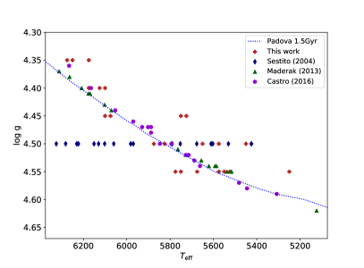
(a) Dwarf Atmosphere Parameters

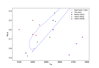
(b) Giant Atmosphere Parameters

Figure 7: $T_{eff}$-log g comparisons between this work and Sestito, Randich & Pallavicini (2004), Reddy, Giridhar & Lambert (2013), Maderak et al.  (2013), Böcek Topcu et al.  (2015), and Castro et al.  (2016). The 1.5 Gyr isochrones are shown as the blue dotted line in both figures. Note that Sestito, Randich & Pallavicini assumed a constant log g of 4.50 for all dwarfs.

Figure 7 plots our final $T_{\rm{eff}}$/log g combinations against other published values for both dwarfs (Figure 7a) and giants (Figure 7b). We also include the 1.5 Gyr PARSEC isochrone at solar metallicity. The difference between selecting a 1.45 Gyr (Anthony-Twarog et al.  2009), 1.6 Gyr (Carrera & Pancino 2011), or our plotted 1.5 Gyr isochrone is less than the typical point size on the plots, and results in log g and $T_{\rm{eff}}$ differences of less than 0.01 and 10K, respectively. It is worth noting that the close fit of the Maderak et al.  (2013) and Castro et al.  (2016) parameter choices to the PARSEC isochrone is due to their choice of using a photometrically-determined $T_{\rm{eff}}$, and selecting their log g value from the corresponding point on an isochrone. Table LABEL:tab:TComps provides a $T_{\rm{eff}}$ comparison between this work and other literature values. The “Delta” column compares the difference between this work and the literature value for a given star while the “Lit. Std.” column shows the standard deviation of the literature values (where available).

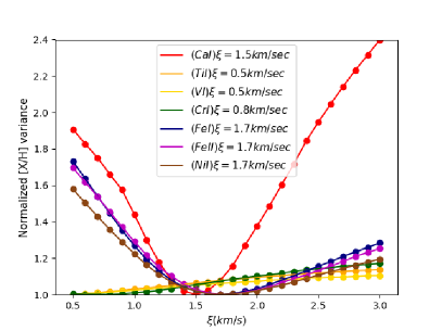
(a) PLA-889 (Main-sequence)

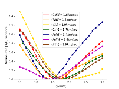
(b) PLA-1089 (Red giant clump)

Figure 8: Normalized line-to-line abundance standard deviation ($\delta$) for various values of micro-turbulent velocity ($\xi$). The [Ca/H] variance best predicts the $\xi$ value corresponding to the minimum variance of the $\delta$-s for the suite of listed elements.

To determine the microturbulent velocity, we calculate the Ca abundance from selected absorption lines, using our previously-determined $T_{\rm{eff}}$ and log g, for a range of $\xi$ values. Our final $\xi$ value for each model is the one where the calculated Ca abundance variance is minimized. Figure 8 illustrates the process for an example star. Note that while this is essentially the same process used in Reddy, Giridhar & Lambert (2012), we selected Ca to determine the minimum variance point, as opposed to th combination of Fe, V, Cr, and Ti in the prior work. The choice of Ca led to the $\xi$ value with the least ambiguity, and Ca absorption lines were consistently available in both giant and main-sequence populations. We also use Fe I]/Fe II and Ti I/Ti II measurements for $T_{\rm{eff}}$ and log g determination.

Our parameters were used to create atmospheric models using the ATLAS9 grids (Castelli & Kurucz 2004). We used a linear interpolation algorithm between the existing grid points, based on our $T_{\rm{eff}}$, log g, and $\xi$ values. Since stellar metallicity is a parameter in determining the proper model, we used an iterative process to select the appropriate value for a given model. Starting with a solar metallicity, we calculated the Fe/H value for a given star, and then repeated the process, using the new metallicity, until we found a stable value. When a general metallicity value was required, notably in isochrone generation, we used a weighted average of our Fe I and Fe II measurements from both giant and dwarf stars. For Fe abundances, we use the notation of $log_{10}({N(Fe)}/{N(H)})+12.00$ where $log_{10}N(H)$ is set at 12.00. We measured the cluster (Fe) metallicity value at $7.49\pm 0.06$. Using the solar value of 7.50 from Asplund et al.  (2009), our cluster metallicity is $[Fe/H]=-0.01\pm 0.06$.

Our EQW measurements and interpolated atmospheric models were used as inputs to the MOOG “abfind”, “blends”, and “synth” drivers, resulting in our final abundance calculations.

3.7 GAIA Reference Spectra Calibration

To verify our abundance calculation methodology, we obtained spectra from The Gaia FGK Benchmark Star archive (Blanco-Cuaresma et al.  2014), supplemented by the low-metallicity sample from Hawkins et al.  (2016). To best match the wavelength coverage and resolution of our NGC 752 spectra from the Keck Archive, we preferentially selected the spectra from the NARVAL (Aurière 2003) (24 spectra) and UVES-POP (Bagnulo et al.  2003) (9 spectra) instruments, with a small number of spectra from the HARPS (Mayor et al.  2003) (4 spectra) and ESPaDOnS (Donati 2003) (2 spectra) instruments.

In order to minimize abundance variances due to atmospheric parameter variation, we adopted the parameters as determined in Heiter et al.  (2015). Using our measurement and calculation techniques described earlier, we derived abundances for our element suite in the 39 reference stars. We then compared our results with those compiled in Jofré et al.  (2015). Figure 10 presents the comparison in graphical form. Each point plots the “literature” abundance (X-Axis) against our measured abundance (Y-axis). In cases where an element was not explicitly measured in Jofré et al. , the literature value is calculated by using the individual star’s [Fe/H], and assuming a solar ratio for [X/Fe] to produce a [X/H] value. The red points in Figure 10 represent the comparison to actual literature values while the blue points are those which use the extrapolated abundances.

Although our software is intended for use with stars of (approximately) solar metallicity, we also include the low metallicity stars of the GAIA reference spectra set with points in a lighter shade (pink/cyan) of their corresponding solar metallicity counterparts.

When comparing individual elemental abundances on a star-to-star basis, our calculated abundances for all stars and elements in the GAIA set (noted as:[X/H]) differed by $-0.03\pm 0.13$. When comparing solar metallicity star abundances that were “directly” measured in the Jofré et al.  compilation, our measurements were also essentially the same, at: $-0.04\pm 0.12$. The same can be said if we analyze the comparison between our measurements and “extrapolated” literature values ($-0.06\pm 0.14$). For the low-metallicity sample, our measured results were also the same as both the directly-measured and extrapolated values: $-0.01\pm 0.12$ and $+0.02\pm 0.14$, respectively. It is important to note that the variance among the literature values when multiple values are given in Jofré et al.  is $\pm 0.10$.

4 Abundance Results

Our abundance results are shown in Table LABEL:tab:752Abs, which contains the cluster averages, with dwarf and giants averaged separately, along with the standard deviation of the individual star measurements, and the count of stars in which a given element was measured. While Fe is measured on the scale of $log_{10}({N(Fe)}/{N(H)})+12.00$, all other elements are measured relative to Fe, as denoted by [X/Fe].

We have chosen to list the standard deviation of the individual line measurements as our uncertainty for the abundance measurement for a given star. While this method produces a larger uncertainty (by a factor of $\sqrt{n-1}$) when compared to the varaince of the mean(s), we find the larger uncertainties are more representative of our measurement techniques. We also note that individual line measurements do not represent truly independant measurements of a star’s elemental abundance, as they can be non-uniformly affected by factors dependant on wavelength (through the reduction process), physical line parameters (excitation potential and log gf, and their associated uncertainties), and equivalent width measurements. The “Q.” score column in is the average of all line quality scores (see Section 3.3) used in calculating the listed abundance.

Individual star data is shown in the extended abundance table, available in the digital version of Table LABEL:tab:752Abs. In order to properly characterize the uncertainty in individual star abundance measurements, caused by varying model atmosphere parameters, we re-ran the full abundance determination process, varying each of the three parameters, as shown in Table LABEL:tab:atmErrs. We then added the largest error of each parameter (either the “+”, or the “-” error) in quadrature, to produce an atmospheric parameter error. Uncertainty, due to variance in line measurements, is designated as $\sigma_{var}$ in Table LABEL:tab:752Abs. Abundance uncertainty, due to uncertainty in atmospheric parameters, is designated as $\sigma_{atm}$ in the same table.

4.1 Iron and Iron-Peak Elements

Our measured Fe abundance was based on over 400 absorption features. As discussed in Section 3.5, the large number of measurements was pared to a smaller subset to eliminate data which were likely affected by measurement errors. Using a weighted average of our calculated Fe I/H (75%) and Fe II/H (25%) for both dwarf and giant members, we derive a cluster (Fe) metallicity of $7.49\pm 0.06$. We use this value for all atmospheric models and isochrones during the abundance and atmospheric parameter determination process.

In addition to Fe I and Fe II, we also measured the four other “Iron Peak” elements, Cr (I and II), Mn I, Co I, Ni I, and two “nearby” elements V I, and Cu I. Composite cluster values are shown in Table LABEL:tab:752Abs, and individual line measurements in the online version of Table LABEL:tab:LineList. As with Fe abundances, we find no significant differences between abundance measures of these elements in the dwarf and giant population. We accounted for the hyperfine structure of V, Mn, and Cu lines by using the MOOG blends driver, with the line component parameters taken from the line sources listed in Table LABEL:tab:LineList. As with Sc I below, we expect the odd-Z element Co to also have hyperfine structure in its line profiles. However, we have no appropriate source to implement these characteristics, and must rely upon an assumed similarity between the NGC-752 stars, and the solar reference counterpart to adjust for this structure.

Our measured abundances for the five elements (V I, Cr I, Fe I, Co I, and Ni I) commonly measured in our study and in the giant studies of Carrera & Pancino (2011) and Reddy, Giridhar & Lambert (2012), match well. Table LABEL:tab:FeGroupComps provides a summary of the five elements over the three studies.

4.2 Carbon, Nitrogen and Oxygen

With the assumed age of 1.45 Gyr, and a Main Sequence Turn Off (MSTO) mass of $1.5M_{\odot}$ (Bartašiūtė et al.  2007), we expect the evolved members of NGC 752 to show evidence of CNO-cycle processing. Even though the CNO processing is ongoing throughout a star’s lifetime, conditions at the core-radiative zone boundary isolate core materials until core hydrogen fusion ends. Convective processes during the H shell fusion, and core He fusion phases allow the altered core materials to mix into the stars’ atmosphere, becoming detectable in our giant star spectra. Iben (1964) and Iben (1991) summarize the atmospheric differences we expect to see as a result of this “first dredge-up”. Specifically, we should expect increases in ¹³C (relative to ¹²C) and ¹⁴N.

While all three light elements are common in stellar atmospheres, measurement is difficult, even with high S/N spectra, due to the lack of low-excitation transitions in optical spectra. Our measurements consist of abundances as calculated from both synthesis and from absorption line feature measurements. Unfortunately, we were unable differentiate between isotope states, particularly ¹²C and ¹³C, so our analysis is based on relative elemental (instead of isotope) measures.

For our giant population, we utilized a combination of elemental and molecular absorption features to calculate C and N abundances. As C-, N-, and O-molecule abundances are inter-related, we first determined the cluster O abundances using equivalent width measurements of several features, including the O I “triplet” at 7771-7776 Å. Figure 3 illustrates the spectral region encompasing the triplet region. While MOOG abundance calculations assume Local Thermal Equilibrium (LTE), we adjusted our final abundances for the expected non-LTE (NLTE) conditions of the high-excitation potentials ($\geq{9.14eV}$), as suggested in Takeda (2003). We find [O I/Fe]$=-0.11\pm 0.08$, with similar abundance measurements in the dwarf and giant populations. The cluster, dwarf, and giant (individual star measures in the digital version of the table) [O/Fe] measurements are compiled in Table-LABEL:tab:752Abs. Our measured [O/Fe] of $-0.15\pm 0.07$ in our giant sample is lower than that of the giants measured by Carrera & Pancino (2011) of $+0.03\pm 0.04$, possibly due to differences in the measurement methods. Carrera & Pancino calculated their O abundances using synthesis around the [O I] forbidden line near 6300Å.

Our abundance determination for C is a composite of equivalent width measurements of the features at 5382 Å, 6381 Å, and 8335 Å and spectral synthesis of the region near 7115 Å, which contains several high-excitation C I absorption features (see Figure 4). The synthesis process was partially iterative between C and N abundances, as there are CN features in the same region. In determining the C abundance, we gave higher priority to fitting the lines at 7111 Å and 7113 Å, since they were more isolated from CN features. Table-LABEL:tab:752Abs lists our [C/Fe] results; [C/Fe]$=-0.10\pm 0.13$ (dwarfs) and [C/Fe]$=-0.22\pm 0.08$ (giants).

Individual EQW measurements were given equal weight, with the abundance calculated from the synthesis given five (5) times the weight of a single EQW measurement (appropriate for the 5 blended lines in that region). While all of our measured C lines have (relatively) high excitation potentials ($>{7.68eV}$), at the effective temperature of our sample stars, we do not expect NLTE effects to be significant (as per Rentzsch-Holm (1996)).

Nitrogen abundance was exclusively calculated using spectral synthesis. As none of our spectra had coverage of the strong CN bandheads in the near-UV and near-IR regions, we used a combination of the N abundance derived during synthesis of the 7115 Å region, and an additional synthesis around the 7442 Å region. Based on the measurement of a single N absorption line in one dwarf spectrum, and sysntesis in the five giant spectra, we find [N/Fe]$=0.12$(1 dwarf) and $0.28\pm 0.07$(giants)

Our measurements of the giant sample show a decrease of C to below that of solar, and N significantly higher. The general pattern of higher N and lower C abundance corresponds to the results of the giants measured by Böcek Topcu et al.  (2015), although our measured C abundance is significantly higher, at $[C/Fe]=-0.22\pm 0.08$ vs. their value of$-0.46\pm 0.03$ probably due to the difference in synthesis region selection. Likewise, our measured N abundance of $+0.27\pm 0.06$ is also higher than that measured by Böcek Topcu et al. , which we partially attribute to the unavailability of the violet and red bands of the CN spectrum.

Böcek Topcu et al.  explain the relative N enhancement and C depletion to main-sequence evolutionary processes, namely He production in the core through the CNO cycle. The relevant portion of the CNO cycle is that which occurs at the lowest temperature:

$${}^{12}C(p,\gamma)^{13}N(,e^{+}\gamma_{e})^{13}C(p,\gamma)\rightarrow$$

$${}^{14}N(p,\gamma)^{15}O(,e^{+}\gamma_{e})^{15}N(p,\alpha)^{12}C$$

The slow step, or “bottleneck”, is the ¹⁴N proton capture. Over the course of the main-sequence lifetime of a star, this results in an increase of N abundance at the expense of the ¹²C abundance. With the MSTO mass of at least $1.5M_{\odot}$, evidence of processing from the higher temperature branch of the CNO-I-cycle (CNO-II) might also be present. Specifically, the high temperature branch has two steps which require proton capture by O. Like the N increase in the CNO-I cycle, increased O abundance might be explained through the capture steps in the higher temperature CNO-II cycle. Since we do not measure an increased O abundance, we conclude that these higher temperature branches are not significant contributors to the elemental alteration of NGC 752’s stars.

Admittedly, measuring the CNO abundances in giant stars only shows half the picture. The critical comparison should occur between main-sequence and evolved members, not between a solar reference and the evolved members. To that end, we have measured C and O abundances using the aformentioned absorption features at 7115 Å and 7775 Å, respectively. These abundance measurements do hint at the expected trend for CNO processing, but measurement uncertainty, particularly due to the lack of strong CN features in our dwarf sample, prevents us from making a definitive statement to that effect.

The third “piece” - N abundance - also shows the expected trend for CNO processing, but again, we would need more, higher resolution spectra to make this claim definite. N abundances are the result of molecular CN feature synthesis, so we were largely unable to determine N abundances for the dwarf population. Our sole dwarf N abundance comes from a single EQW measurement of the 7442.29 Å N I feature in PLA-520. We also recorded similar measurements from PLA-859 and PLA-889, but disqualified them due to their EQW measurements falling below the acceptable minimum width threshold for the respective spectra’s S/N ratio. We also note that the [C/N] ratio of -0.50, as measured in our giant sample, agrees well with the expected [C/N] of -0.54 for a 1.5Gyr giant just after its first dredge-up ([C/N]_FDU) at solar metallicity given in Salaris et al.  (2015).

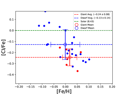
(a) Carbon

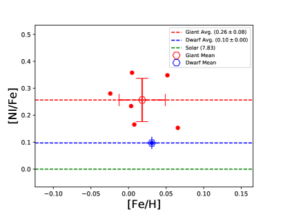
(b) Nitrogen

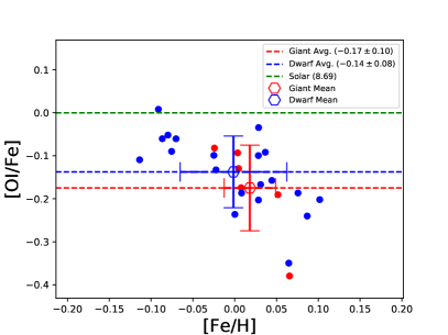
(c) Oxygen

Figure 11: Individual star abundances for C I, N I, and O I. The abundance mean for the dwarf population is designated by the blue hexagon, and the giants in red.

Figure 11 shows the summary results of our C and O light-element measurements. Individual star measurements are compiled in the digital version of Table LABEL:tab:752Abs.

4.3 Light Elements

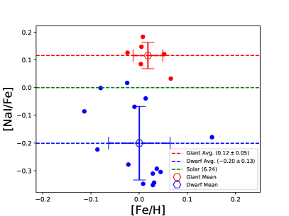
(a) Sodium

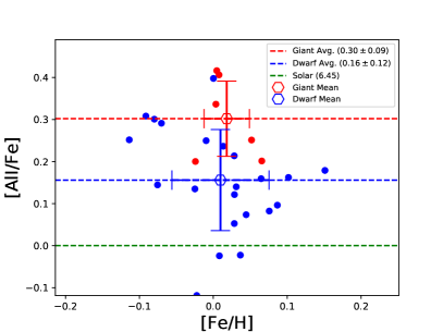
(b) Aluminium

Figure 12: Individual star abundances for the odd-Z light elements, Na I, and Al I. The abundance mean for the dwarf population is designated by the blue hexagon, and the giants in red.

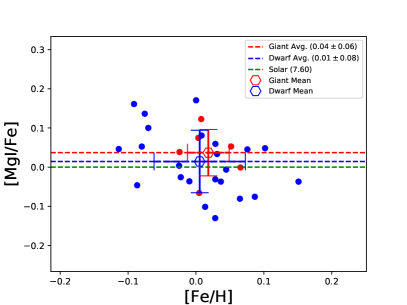
(a) Magnesium

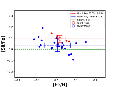
(b) Silicon

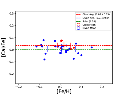
(c) Calcium

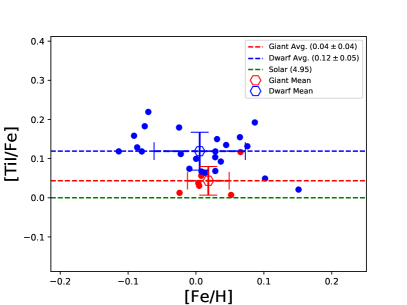
(d) Titanium

Figure 13: Individual star abundances for the alpha-elements, Mg I, Si I, Ca I, and Ti I. The abundance mean for the dwarf population is designated by the blue hexagon, and the giants in red.

The “light” elements, with $11\leq{Z}\leq 22$, provide viable targets for measurement, even with our lowest S/N spectra. Na, Mg, Al, Si, Ca, and Ti all have either a large number of measureable transitions, or strong, well documented features. We find that, within our error margins, the abundance of these elements follow their solar counterparts. We chose to separate the elements into two groups for discussion. Our odd-Z light element sample of Na I and Al I are shown in Figure 12. While both light elements show significant star-to-star variation, Na appears to be enhanced in the giants, while Al is likely unchanged. The “$\alpha$-”, or even-Z elements (Mg I, Si I, Ca I, and Ti I), as shown in Figure 13, potentially show evidence of evolution. Silicon abundance appears to increase, from $0.05\pm 0.05$ in the dwarf population to $0.11\pm 0.02$ in the giants, while Ti appears to decrease ($0.13\pm 0.05$ to $0.06\pm 0.04$). However, both of these changes are within the $1-\sigma$ error bars, and would need more accurate measurements to show a definite trend.

When comparing Na abundances between the dwarf and giant population, we find an increase from [Na/Fe]$=-0.18\pm 0.12$ to $0.13\pm 0.05$. For both dwarf and giant samples, we applied the NLTE Na corrections from Lind et al.  (2011) using the calculator at: http://inspect.coolstars19.com/cp/application.py/A_from_e?element_name=Na Our measured Na increase in the giants is possibly due to the same mechanism as Boesgaard, Roper & Lum (2013) noted in comparing their Praesepe dwarf population with the giants studied by Carrera & Pancino (2011). Specifically, that the enrichment is a result of the NeNa cycle as detailed in Arnould & Mowlavi (1995). As with the O and N enhancement during CNO processing, the ²³Na proton capture has the smallest cross-section, which provides an explanation for our measured enhancement.

Arnould & Mowlavi and Ventura, Carini & D’Antona (2011) also discuss Al enhancement through the MgAl cycle. While Ventura, Carini & D’Antona specifically address the MgAl cycle in AGB stars, the conditions in the core during the “He-flash” can easily reach the necessary conditions for the process to occur. When comparing our dwarf and giant populations, the measured Al abundances differ by less than the star-to-star variance, but possibly show an increase (from dwarfs $0.17\pm 0.11$ to giants $0.32\pm 0.09$). However, we do not measure significant decrease in Mg, the depleted element in the MgAl cycle, between our two populations. As with Boesgaard, Roper & Lum, we may even measure an increase in Mg in the giants. This is not entirely unexpected, as the ${}^{23}Na(p,\gamma)^{24}Mg$ step within the NeNa cycle can provide a “leakage” of Mg, resulting in an abundance increase. Ventura, Carini & D’Antona also state that increases in Si as a result of the MgAl cycle are possible. More than with our Al and Mg measurements, the giant Si abundance shows an increase, corresponding to that expected in Ventura, Carini & D’Antona, but star-to-star variances and the lack of evidence for Mg depletion prevent us from making the definitive statement that the Si increase is a result of such cycling.

Our abundance measures for both Sc II, V I and V II are included in Table LABEL:tab:752Abs, and show consistent measures between the two populations.

4.4 Heavy Elements

We have also included measurements of several elements with $Z\geq 30$. Generally speaking, high-Z elements track slightly above solar ratios. While s-process enhancement of elements with N=50 (Y) and N=80 (Ba, and Ce to a lesser extent) is possible, the availability of neutron flux relies on higher temperature reactions. These reactions, ${}^{13}C(\alpha,n)^{16}O$ and ${}^{22}Ne(\alpha,n)^{25}Mg$, occur at approximately $1.5x10^{8}$ and $3x10^{8}K$, respectively (Kaeppeler et al.  1990) - temperatures which we do not expect our target star cores to reach. While our sample giant stars have not yet reached the Assymptotic Giant Branch (AGB) phase where these reactions could proceed, the He degeneracy fraction prior to the He-flash may allow core temperatures to reach the threshold for these n-generating processes to proceed. However, since we do not measure a significant abundance increase in the end products, O and Mg, of the neutron generating process, we would not expect to see the results from s-processing. Correpondingly, we did not find a significant change in the abundances of the heavy, s-process elements, Y and Ba, and to a lesser extent, Ce, which are included in Table LABEL:tab:752Abs. Our Sm II abundances, at first glance, would indicate a significant decrease in the abundance of the element. However, this does not hold up to scrutiny - the four values from the dwarf population are based on EQW measurements barely above our measurement threshold of 2mÅ. Similar to the weak N I feature, we did produce five additional measurements of Sm abundances, but did not include them due to the EQW measures falling below our 2mÅ minimum threshold for EQW measurements. If we do include these abundances in our dwarf population, the apparent difference between the dwarf and giant population disappears. Therefore, when measuring Sm in this cluster, we would only rely on EQW measures from the giant population, arriving at a cluster value of [Sm/H]=$+0.05\pm 0.03$. Individual star abundance measurements on an element-by-element basis are in the digital version of Table LABEL:tab:752Abs, and the even more detailed individual EQW measures for each line in every star are listed in the included digital material.

5 Summary and Conclusions

Using spectra obtained from public archive data, we have computed atmospheric elemental composition of 23 main sequence stars and 5 red-giant “clump” stars in the open cluster NGC 752. Using an automated process, we determined atmospheric parameters, measured absorption line equivalent widths, and calculated elemental abundances for 25 elements, 7 with multiple ionization states. We enhanced the accuracy of our abundance calculations by using a substantially larger set of line measurements, and an automated measurement process which removed the subjective element from the equivalent width measurement process. This process also performs a line quality assessment, by comparing the abundance calculated from our automated process in a high-resolution solar spectrum, with the “known” values in Asplund et al.  (2009).

Overall, the cluster abundances track closely with their solar counterparts, with very slight enhancement ([X/Fe]$<+0.05$ dex) of most elements, relative to Fe. We find a cluster Fe abundance of $7.49\pm 0.06$ ($[Fe/H]=-0.01\pm 0.06$), with no differences between giant and dwarf, and/or Fe I and Fe II measurements. Similarly, the abundances of the other iron-peak elements follow their solar counterparts, and do not differ between the dwarf and giant populations ([Cr/Fe]$=0.04\pm 0.06$, [Mn/Fe]$=-0.01\pm 0.04$, [Co/Fe]$=0.11\pm 0.07$, and [Ni/Fe]$=-0.02\pm 0.04$).

Since our sample population contained both dwarf and giant stars, we looked for evidence of nucleosynthetic processing, including CNO cycling. We find that C I is slightly depleted ([C/Fe]$=-0.10\pm 0.13$) in the dwarfs, moreso in the giants ($-0.22\pm 0.08$). We measured a N I enhancement in the giant population ($+0.28\pm 0.07$), whereas O I is consistent between the dwarfs and giants ($-0.10\pm 0.08$, and $-0.15\pm 0.07$, respectively). The combination of C depletion with N enhancement, is evidence of CNO cycling during the main-sequence lifetime of the evolved stars.

We also found evidence of the NeNa light element “cycle”. We measured a Na enhancement in the giants ($+0.13\pm 0.05$), and slight depletion in the dwarfs ($-0.18\pm 0.12$). We did not find evidence of the hotter MgAl cycle, as the dwarf and giant populations measured the same Mg and Al abundances (within errors), with only a slight increase in Si (a possible secondary product of the MgAl cycle) abundance.

We find no evidence for enhancement of $\alpha$-elements (O, Mg, Si, Ca, Ti). The group show only slight to no enhancement ($<0.05$ dex) over either solar ratios, or between dwarfs and giants.

We also sampled a number of heavier (Z$\geq 29$) elements. While several had slight abundance differences between dwarfs and giants, we do not attribute it to the “slow” neutron capture process (s-process), due to the lack of enhancement of the two high-Z elements with low cross-sections, Y and Ba, as well as lack of evidence of the requisite neutron-producing reactions.

6 Acknowledgements

We would like to thank Fabio Bresolin, Roberto Mendez, and Rolf-Peter Kudritzki for their questions, feedback and suggestions, which greatly improved the quality of this work.

This research has made use of the Keck Observatory Archive (KOA), which is operated by the W. M. Keck Observatory and the NASA Exoplanet Science Institute (NExScI), under contract with the National Aeronautics and Space Administration.

We are extremely grateful to the principal investigators (PIs) of the original observations of the archived data used in our research: J. Cohen, B.Jones, G. Marcy, and S. Schuler. We also wish to thank the maintainers of the digital online archives for their respective instruments, and the observatories and staff for the archives and instruments. When available, we include any requested attributions, below.

This work has made use of the VALD database, operated at Uppsala University, the Institute of Astronomy RAS in Moscow, and the University of Vienna.

This publication makes use of data products from the Two Micron All Sky Survey, which is a joint project of the University of Massachusetts and the Infrared Processing and Analysis Center/California Institute of Technology, funded by the National Aeronautics and Space Administration and the National Science Foundation.

We acknowledge the ESO’s HARPS and UVES staff and archives for providing our solar calibration spectra.

The National Solar Observatory provided our solar baseline spectrum.

Table 1: NGC 752 Archive Observations

Reference Number			RA (J2000)	Dec (J2000)	Wavelength	S/N		Date of	Observer
Pla.	Hen.	Rohlfs	(hh:mm:ss)	(Deg:mm:ss)	Range (Å)	6200 Å	7800 Å	Obs.	Inits.
Dwarfs
300	—	487	01:55:27	+38:08:32	4350-6860	60	—	2000-10-08	BJ
361	29	310	01:55:44	+37:54:31	4350-6860	50	—	2000-10-08	BJ
391	38	313	01:55:53	+37:49:26	6240-8680	—	70	2000-10-09	BJ
413‡	48	294	01:55:59	+37:40:49	6240-8680	—	70	2000-10-09	BJ
429	54	288	01:56:04	+37:36:42	6240-8680	—	70	2000-10-09	BJ
520	80	290	01:56:23	+37:38:14	5650-8090	150	130	2003-11-02	AB
552‡	87	280	01:56:32	+37:34:33	6240-8680	—	60	2000-10-09	BJ
575	94	303	01:56:36	+37:45:35	6240-8680	—	40	2000-10-09	BJ
699∗	144	437	01:57:04	+38:07:20	4350-6860	70	—	2000-10-08	BJ
					5650-8090	150	130	2003-11-02	AB
701	146	260	01:57:06	+37:50:43	6240-8680	—	60	2000-10-09	BJ
					5650-8090	90	80	2003-11-02	AB
					4000-8490	90	130	2009-08-27	JC
					4000-8490	90	120	2009-08-27	JC
786	183	270	01:57:22	+37:38:21	4350-6860	70	—	2000-10-09	BJ
					4000-8490	90	130	2009-08-27	JC
					4000-8490	80	120	2009-08-27	JC
790	185	—	01:57:24	+37:52:12	5650-8090	160	140	2003-11-02	AB
791	184	434	01:57:24	+38:06:10	5650-8090	150	130	2003-11-02	AB
828	199	266	01:57:34	+37:42:01	6240-8680	70	—	2000-10-09	BJ
859∗∗	207	252	01:57:38	+37:49:44	6240-8680	70	—	2000-10-09	BJ
					4000-8490	110	140	2009-08-27	JC
					4000-8490	70	100	2009-08-27	JC
864	211	430	01:57:39	+38:08:39	6240-8680	—	40	2000-10-09	BJ
					5650-8090	150	130	2003-11-02	AB
889	216	427	01:57:45	+38:11:07	6240-8680	—	30	2000-10-09	BJ
					5650-8090	150	130	2003-11-02	AB
921	229	103	01:57:52	+37:27:46	5650-8090	160	140	2003-11-02	AB
964	244	388	01:58:03	+38:02:30	5650-8090	130	120	2003-11-02	AB
993	256	101	01:58:09	+37:28:36	6240-8680	—	60	2000-10-09	BJ
999	—	107	01:58:11	+37:23:53	6240-8680	—	70	2000-10-09	BJ
1012	—	118	01:58:13	+37:15:20	5650-8090	150	120	2003-11-02	AB
1017	265	240	01:58:16	+37:33:26	6240-8680	—	70	2000-10-09	BJ
1107	298	232	01:58:34	+37:40:19	6240-8680	—	70	2000-10-09	BJ
1270	—	—	01:59:19	+37:49:50	6240-8680	—	70	2000-10-09	BJ
1284‡	—	—	01:59:20	+37:23:23	6240-8680	—	70	2000-10-09	BJ
					4000-8490	100	140	2009-08-27	JC
					4000-8490	110	150	2009-08-27	JC
1365	—	187	01:59:47	+37:49:48	4350-6860	35	—	2000-10-08	BJ
Giants
350	24	25	01:55:40	+37:52:28	3360-8100	55	70	2008-06-20	GM
					3360-8100	160	220	2008-06-22†	GM
356	20	27	01:55:43	+37:37:39	3360-8100	55	60	2008-06-20†	GM
					3360-8100	160	220	2008-06-22	GM
506	29	75	01:56:19	+37:58:02	4690-9140	290	400	2009-10-08	SS
687	—	137	01:57:04	+38:07:57	3360-8100	50	70	2008-06-20	GM
					3360-8100	160	220	2008-06-22	GM
					4690-9140	350	450	2009-10-08	SS
1089	67	295	01:58:30	+37:51:37	3360-8100	50	70	2008-06-20	GM
					4690-9140	290	400	2009-10-08	SS
1172	65	311	01:58:53	+37:48:57	3360-8100	50	80	2008-06-20	GM
* - Possible single-line binary								AB- Boesgaard
$\dagger$ - Possible mis-aligned order fit (see text)								JC- Cohen
$\ddagger$ - Spectroscopic Binary (unused)								BJ- Jones
** - Parallax differential (unused)								GM- Marcy
								SS- Schuler

Table 2: NGC 752 Atmospheric Parameters

PLA #	$T_{eff}$	log g	$\xi$	$min.EQW$
	(K)		(km s-1)	(mÅ)
Dwarfs
300	5650	4.50	2.1	12.5
361	5550	4.55	1.8	8.3
391	5450	4.55	1.8	6.3
429	5250	4.55	1.8	6.5
520	6100	4.40	1.6	2.6
575	5525	4.55	1.8	8.8
699	5875	4.50	1.6	2.7
701	5725	4.45	1.7	1.5*
786	5575	4.50	2.0	1.6*
790	6250	4.35	2.1	3.0
791	6125	4.40	1.8	3.0
828	5425	4.50	1.9	6.3
864	6050	4.45	1.7	3.0
889	6175	4.35	1.7	3.0
921	6100	4.45	1.6	2.7
964	6100	4.45	1.6	3.6
993	5675	4.55	1.4	6.5
999	5750	4.45	1.4	5.8
1012	6275	4.35	1.7	3.3
1017	5775	4.55	1.6	6.0
1107	5750	4.55	1.7	5.6
1270	5575	4.55	1.8	5.6
1365	5825	4.50	1.4	11.2
Giants
350	5000	2.65	1.6	1.9*
356	4950	2.60	1.5	1.9*
506	4975	2.65	1.5	1.1*
687	5000	2.65	1.5	0.7*
1089	5100	2.60	1.5	1.0*
1172	5000	2.55	1.6	4.0
*-Adjusted to minimum of 2.0 mÅ

Table 3: Effective Temperature Comparison

PLA ID	This Work	Hobbs	Bala.	Sest.	Biaz.	Made.	Phot.	Lit. Mean	Delta	Lit. Std
300	5650							n/a	n/a	n/a
350	5000				5006			5006	-6	n/a
356	4950				5017			5017	-67	n/a
361	5550					5537		5537	13	n/a
391	5450					5517		5517	-67	n/a
429	5250					5124		5124	126	n/a
506	4975				5009			5009	-34	n/a
520	6100			6151	5999	6102	6102	6089	12	64
575	5525	5350		5425				5388	138	53
687	5000				5010			5010	-10	n/a
699	5875			5970	5754		5899	5874	1	110
701	5725	5690	5693	5677	5722	5656	5674	5685	40	22
786	5575			5531	5653	5517		5567	8	75
790	6250	6220		6325	5992	6264	6248	6210	40	128
791	6125				6076	6208	6198	6161	-36	73
828	5425							n/a	n/a	n/a
864	6050			6060	6021	6071	6073	6056	-6	24
889	6175			6231	6091	6177	6169	6167	8	58
921	6100	5870	6160	6223	6081	6169	6162	6111	-11	126
964	6100			6102	6048		6059	6070	30	29
993	5675			5611		5593		5602	73	13
999	5750					5728		5728	22	n/a
1012	6275			6282	6217		6212	6237	38	39
1017	5775	5740	5760	5791		5764		5764	11	21
1089	5100				5081			5081	19	n/a
1107	5750			5791		5764		5778	-28	19
1172	5000				4975			4975	25	n/a
1270	5575					5621		5621	-46	n/a
1365	5825			5603	5912	5586		5700	125	184
References:
Hobbs: Hobbs & Pilachowski (1986)
Bala.: Balachandran (1995)
Sest.: Sestito, Randich & Pallavicini (2004)
Biaz.: Biazzo et al.  (2007)
Made.: Maderak et al.  (2013)
Phot.: Photometric value as calculated by Cummings et al.  (2017),
	using photometry from Daniel et al.  (1994).

Table 4: Absorption Line List

	Wavelength	Ex. Pot.
Ion	(Å)	(eV)	$Log(gf)$	Ref.∗
C I	5380.340	7.68	-1.62	58
C I	6587.620	8.53	-1.00	23
C I	7100.130	8.64	-1.02	23
C I	7111.450	8.64	-1.08	23
C I	7113.170	8.65	-0.77	23
C I	7115.170	8.64	-1.47	23, 59
…
*-See Table:LABEL:tab:LineRefs for reference key

Table 5: Absorption Line References

Ref.		Ref.
No.	Reference	No.	Reference
1	Allen & Porto de Mello (2011)	35	Garz (1973)
2	Allende Prieto & Garcia Lopez (1998)	36	Giridhar & Arellano Ferro (1995)
3	Bard, Kock & Kock (1991)	37	Hannaford et al.  (1982)
4	Bard & Kock (1994)	38	Kock & Richter (1968)
5	Beveridge & Sneden (1994)	39	Kramida et al.  (2014)
6	Biemont et al.  (1991)	40	Kroll & Kock (1987)
7	Biemont & Godefroid (1980)	41	Lambert & Warner (1968)
8	Bizzarri et al.  (1993)	42	Lambert & Luck (1978)
9	Blackwell, Shallis & Simmons (1980)a	43	Lawler & Dakin (1989)
10	Blackwell et al.  (1986)a	44	Lawler et al.  (2013)
11	Blackwell et al.  (1986)b	45	Lawler et al.  (2008)
12	Blackwell et al.  (1986)c	46	Lawler, Sneden & Cowan (2015)
13	Blackwell, Menon & Petford (1983)	47	Lawler et al.  (2009)
14	Blackwell et al.  (1982)a	48	Lawler et al.  (2014)
15	Blackwell, Petford & Simmons (1982)d	49	Martin, Fuhr & Wiese (1988)
16	Blackwell et al.  (1976)	50	McWilliam & Rich (1994)
17	Blackwell et al.  (1979)a	51	McWilliam et al.  (1995)
18	Blackwell, Petford & Shallis (1979)b	52	Meylan et al.  (1993)
19	Blackwell et al.  (1980)b	53	Moity (1983)
20	Blackwell et al.  (1982)b	54	Nissen & Schuster (1997)
21	Blackwell et al.  (1982)c	55	O’Brian et al.  (1991)
22	Blackwell, Menon & Petford (1984)	56	Prochaska et al.  (2000)
23	Boesgaard, Roper & Lum (2013)	57	Prochaska et al.  (2000)
24	Booth et al.  (1984)	58	Ramírez & Allende Prieto (2011)
25	Buurman et al.  (1986)	59	Reddy, Giridhar & Lambert (2013)
26	Cardon et al.  (1982)	60	Savanov, Huovelin & Tuominen (1990)
27	Cohen et al.  (2003)	61	Schnabel, Kock & Holweger (1999)
28	Den Hartog et al.  (2014)	62	Smith & Raggett (1981)
29	Den Hartog et al.  (2011)	63	Sobeck, Lawler & Sneden (2007)
30	Edvardsson et al.  (1993)	64	Stephens (1999)
31	Francois (1988)	65	Wickliffe & Lawler (1997)
32	Fry & Carney (1997)	66	Wiese & Martin (1980)
33	Fuhr, Martin & Wiese (1988)	67	Wood et al.  (2013)
34	Fuhrmann, Axer & Gehren (1995)	68	Wood et al.  (2014)

Table 6: Solar absorption line quality evaluation

Ion	Asplund (2009)	$\Delta\leq 0.05$	$\Delta\leq 0.10$	$\Delta\leq 0.20$	$\Delta\leq 0.40$	$\Delta\leq 1.00$	All lines
C I	8.43$\pm$0.05	8.44$\pm$0.02 (3)	8.42$\pm$0.04 (4)	8.41$\pm$0.09 (6)	8.47$\pm$0.13 (8)	8.55$\pm$0.25 (9)	8.55$\pm$0.25 (9)
O I	8.69$\pm$0.05	8.69$\pm$0.02 (2)	8.72$\pm$0.05 (3)	8.77$\pm$0.06 (6)	8.77$\pm$0.06 (6)	8.84$\pm$0.18 (7)	8.84$\pm$0.18 (7)
Na I	6.24$\pm$0.04	6.26$\pm$0.01 (2)	6.26$\pm$0.01 (2)	6.27$\pm$0.08 (5)	6.23$\pm$0.12 (6)	6.36$\pm$0.32 (7)	6.36$\pm$0.32 (7)
Mg I	7.60$\pm$0.04	7.62$\pm$0.02 (6)	7.61$\pm$0.05 (10)	7.60$\pm$0.07 (12)	7.60$\pm$0.07 (12)	7.48$\pm$0.27 (15)	7.20$\pm$0.91 (17)
Al I	6.45$\pm$0.03	6.42$\pm$0.00 (1)	6.41$\pm$0.01 (2)	6.35$\pm$0.06 (4)	6.31$\pm$0.08 (6)	6.31$\pm$0.08 (6)	6.31$\pm$0.08 (6)
Si I	7.51$\pm$0.03	7.53$\pm$0.03 (8)	7.52$\pm$0.05 (16)	7.57$\pm$0.10 (33)	7.59$\pm$0.11 (37)	7.62$\pm$0.15 (40)	7.71$\pm$0.41 (42)
Si II	7.51$\pm$0.03	—	—	7.70$\pm$0.00 (2)	7.70$\pm$0.00 (2)	7.70$\pm$0.00 (2)	7.70$\pm$0.00 (2)
S I	7.12$\pm$0.03	—	—	7.27$\pm$0.00 (1)	7.37$\pm$0.10 (2)	7.37$\pm$0.10 (2)	7.37$\pm$0.10 (2)
Ca I	6.34$\pm$0.04	6.31$\pm$0.01 (3)	6.32$\pm$0.05 (5)	6.32$\pm$0.14 (14)	6.23$\pm$0.21 (29)	6.15$\pm$0.27 (35)	6.15$\pm$0.27 (35)
Sc I	3.15$\pm$0.04	—	3.22$\pm$0.00 (1)	3.19$\pm$0.13 (5)	3.18$\pm$0.19 (7)	3.18$\pm$0.19 (7)	3.18$\pm$0.19 (7)
Sc II	3.15$\pm$0.04	3.14$\pm$0.01 (4)	3.15$\pm$0.05 (7)	3.15$\pm$0.09 (11)	3.16$\pm$0.15 (13)	3.19$\pm$0.18 (14)	3.19$\pm$0.18 (14)
Ti I	4.95$\pm$0.05	4.95$\pm$0.03 (60)	4.94$\pm$0.05 (103)	4.94$\pm$0.10 (166)	4.97$\pm$0.19 (255)	5.09$\pm$0.36 (344)	5.55$\pm$0.96 (471)
Ti II	4.95$\pm$0.05	4.94$\pm$0.03 (9)	4.96$\pm$0.06 (16)	4.97$\pm$0.10 (25)	4.95$\pm$0.21 (41)	5.03$\pm$0.36 (54)	5.13$\pm$0.69 (59)
V I	3.93$\pm$0.08	3.92$\pm$0.02 (24)	3.94$\pm$0.05 (40)	3.95$\pm$0.09 (58)	3.94$\pm$0.12 (64)	3.96$\pm$0.15 (66)	3.99$\pm$0.28 (67)
V II	3.93$\pm$0.08	3.92$\pm$0.00 (1)	3.88$\pm$0.04 (2)	3.86$\pm$0.04 (3)	3.79$\pm$0.13 (4)	3.79$\pm$0.13 (4)	3.79$\pm$0.13 (4)
Cr I	5.64$\pm$0.04	5.63$\pm$0.03 (20)	5.62$\pm$0.06 (46)	5.63$\pm$0.11 (78)	5.63$\pm$0.16 (100)	5.68$\pm$0.33 (130)	5.79$\pm$0.58 (141)
Cr II	5.64$\pm$0.04	5.63$\pm$0.03 (2)	5.64$\pm$0.06 (4)	5.67$\pm$0.10 (7)	5.62$\pm$0.20 (12)	5.58$\pm$0.29 (15)	5.58$\pm$0.29 (15)
Mn I	5.43$\pm$0.05	5.43$\pm$0.02 (5)	5.41$\pm$0.06 (11)	5.36$\pm$0.08 (20)	5.34$\pm$0.09 (23)	5.34$\pm$0.09 (23)	5.41$\pm$0.34 (24)
Fe I	7.50$\pm$0.04	7.49$\pm$0.03 (49)	7.49$\pm$0.05 (79)	7.47$\pm$0.10 (148)	7.39$\pm$0.19 (265)	7.32$\pm$0.30 (355)	7.32$\pm$0.39 (368)
Fe II	7.50$\pm$0.04	7.50$\pm$0.04 (12)	7.49$\pm$0.05 (22)	7.48$\pm$0.09 (35)	7.43$\pm$0.15 (46)	7.37$\pm$0.27 (56)	7.34$\pm$0.32 (58)
Co I	4.99$\pm$0.07	4.99$\pm$0.03 (19)	4.96$\pm$0.05 (33)	4.96$\pm$0.09 (50)	4.99$\pm$0.17 (66)	5.08$\pm$0.37 (92)	5.69$\pm$1.10 (130)
Ni I	6.22$\pm$0.04	6.22$\pm$0.03 (29)	6.23$\pm$0.06 (62)	6.24$\pm$0.10 (97)	6.23$\pm$0.16 (125)	6.22$\pm$0.29 (150)	6.29$\pm$0.51 (158)
Cu I	4.19$\pm$0.04	4.16$\pm$0.00 (1)	4.18$\pm$0.08 (3)	4.18$\pm$0.08 (3)	4.23$\pm$0.12 (4)	4.31$\pm$0.19 (5)	4.31$\pm$0.19 (5)
Zn I	4.56$\pm$0.05	—	4.65$\pm$0.00 (2)	4.67$\pm$0.03 (3)	4.67$\pm$0.03 (3)	4.67$\pm$0.03 (3)	4.67$\pm$0.03 (3)
Y I	2.21$\pm$0.05	—	—	—	2.43$\pm$0.00 (1)	2.63$\pm$0.21 (2)	2.63$\pm$0.21 (2)
Y II	2.21$\pm$0.05	2.20$\pm$0.01 (2)	2.17$\pm$0.04 (3)	2.26$\pm$0.09 (7)	2.34$\pm$0.19 (14)	2.25$\pm$0.29 (16)	2.25$\pm$0.29 (16)
Zr I	2.58$\pm$0.04	2.55$\pm$0.00 (1)	2.59$\pm$0.05 (2)	2.64$\pm$0.11 (6)	2.66$\pm$0.11 (7)	2.66$\pm$0.11 (7)	2.66$\pm$0.11 (7)
Zr II	2.58$\pm$0.04	2.56$\pm$0.00 (1)	2.56$\pm$0.00 (1)	2.56$\pm$0.00 (1)	2.56$\pm$0.00 (1)	2.56$\pm$0.00 (1)	2.56$\pm$0.00 (1)
Ba II	2.18$\pm$0.09	—	—	2.03$\pm$0.04 (2)	2.15$\pm$0.17 (3)	2.04$\pm$0.24 (4)	1.84$\pm$0.46 (5)
Ce II	1.58$\pm$0.04	1.61$\pm$0.01 (3)	1.59$\pm$0.06 (8)	1.61$\pm$0.08 (9)	1.65$\pm$0.15 (14)	1.68$\pm$0.17 (15)	1.93$\pm$1.00 (16)
Pr II	0.72$\pm$0.04	—	—	—	—	1.60$\pm$0.00 (1)	1.60$\pm$0.00 (1)
Nd II	1.42$\pm$0.04	1.42$\pm$0.02 (8)	1.42$\pm$0.03 (10)	1.45$\pm$0.07 (12)	1.47$\pm$0.11 (13)	1.52$\pm$0.20 (14)	1.52$\pm$0.20 (14)
Sm II	0.96$\pm$0.04	0.96$\pm$0.00 (1)	1.02$\pm$0.04 (4)	1.02$\pm$0.04 (4)	1.09$\pm$0.11 (6)	1.15$\pm$0.17 (7)	1.15$\pm$0.17 (7)
Eu II	0.52$\pm$0.04	—	0.45$\pm$0.00 (1)	0.45$\pm$0.00 (1)	0.45$\pm$0.00 (1)	0.71$\pm$0.26 (2)	0.71$\pm$0.26 (2)

Table 7: Elemental Abundances for NGC 752:
Fe I and Fe II abundances are listed on the scale $log_{10}({N(Fe)}/{N(H)})+12.00$ where $log_{10}N(H)$ is set at 12.00, as stated in the text. Listed abundance errors are the star-to-star variations ($\sigma_{var}$) and the atmospheric errors ($\sigma_{atm}$) from Table LABEL:tab:atmErrs. The atmospheric errors for “All Stars” abundances are the mean of the dwarf and giant stars, weighted by population. The “Q.” (quality) score is the average of all measured lines for a given element (see section 3.4). Quality scores for synthesized measurements are listed as “n/a”.

	All Stars					Dwarfs					Giants
Ion	Ab.	$\sigma_{var}$	$\sigma_{atm}$	#	Q.	Ab.	$\sigma_{var}$	$\sigma_{atm}$	#	Q.	Ab.	$\sigma_{var}$	$\sigma_{atm}$	#	Q.
Fe I	7.50	0.06	0.08	29	8.0	7.50	0.07	0.08	23	8.1	7.51	0.03	0.11	6	7.9
Fe II	7.45	0.06	0.06	29	8.5	7.45	0.07	0.05	23	8.6	7.45	0.05	0.10	6	7.8
[C I/Fe]	-0.13	0.13	0.13	27	n/a	-0.10	0.13	0.02	21	0.5	-0.22	0.08	0.02	6	n/a
[N I/Fe]	0.25	0.08	0.01	7	n/a	0.12	n/a	0.08	1	1.0	0.28	0.07	0.00	6	n/a
[O I/Fe]	-0.11	0.08	0.10	26	8.3	-0.10	0.08	0.10	20	8.0	-0.15	0.07	0.11	6	9.1
[Na I/Fe]	-0.09	0.18	0.07	20	8.6	-0.18	0.12	0.06	14	8.0	0.13	0.05	0.09	6	10.0
[Mg I/Fe]	0.04	0.07	0.04	29	9.2	0.03	0.07	0.04	23	9.0	0.05	0.07	0.05	6	9.8
[Al I/Fe]	0.20	0.12	0.06	28	9.9	0.17	0.11	0.05	22	9.8	0.32	0.09	0.08	6	10.0
[Si I/Fe]	0.07	0.05	0.03	29	7.6	0.05	0.05	0.02	23	7.6	0.11	0.02	0.06	6	7.7
[Ca I/Fe]	0.02	0.04	0.10	29	6.6	0.02	0.04	0.09	23	6.4	0.05	0.03	0.12	6	7.2
[Sc II/Fe]	0.00	0.07	0.03	27	8.7	-0.02	0.07	0.02	21	8.9	0.04	0.03	0.08	6	8.0
[Ti I/Fe]	0.11	0.05	0.11	29	8.2	0.13	0.05	0.10	23	8.2	0.06	0.04	0.14	6	8.0
[Ti II/Fe]	0.09	0.10	0.03	27	8.5	0.11	0.11	0.02	21	8.6	0.04	0.05	0.09	6	7.9
[V I/Fe]	0.12	0.09	0.12	20	8.6	0.12	0.10	0.11	14	8.7	0.13	0.05	0.16	6	8.5
[V II/Fe]	0.19	0.12	0.12	17	8.1	0.21	0.12	0.02	11	7.1	0.15	0.10	0.04	6	9.8
[Cr I/Fe]	0.06	0.06	0.08	29	8.3	0.06	0.07	0.08	23	8.4	0.05	0.02	0.09	6	7.9
[Cr II/Fe]	-0.06	0.07	0.09	13	7.9	-0.03	0.07	0.05	7	8.0	-0.10	0.06	0.10	6	7.7
[Mn I/Fe]	-0.01	0.05	0.09	18	7.1	-0.03	0.04	0.08	12	6.7	0.04	0.02	0.11	6	7.8
[Co I/Fe]	0.11	0.07	0.09	29	8.5	0.11	0.08	0.08	23	8.5	0.11	0.04	0.11	6	8.4
[Ni I/Fe]	-0.02	0.04	0.07	29	7.8	-0.03	0.04	0.07	23	7.8	0.00	0.01	0.08	6	7.9
[Cu I/Fe]	-0.06	0.06	0.06	22	7.7	-0.06	0.06	0.06	22	7.7	—	—	—	0	—
[Zn I/Fe]	-0.16	0.11	0.05	20	8.0	-0.21	0.09	0.03	14	8.0	-0.06	0.08	0.14	6	8.0
[Y II/Fe]	0.02	0.13	0.05	20	7.0	0.01	0.15	0.03	14	6.1	0.05	0.07	0.09	6	9.1
[Zr II/Fe]	-0.01	0.15	0.02	10	10.0	0.09	0.17	0.01	4	10.0	-0.08	0.09	0.04	6	10.0
[Ba II/Fe]	-0.14	0.06	0.09	18	6.0	-0.17	0.03	0.09	12	6.0	-0.08	0.07	0.08	6	6.0
[Ce II/Fe]	0.06	0.12	0.04	13	9.2	0.06	0.16	0.02	7	9.5	0.07	0.03	0.06	6	8.8
[Nd II/Fe]	0.22	0.10	0.03	13	9.4	0.27	0.11	0.03	7	9.5	0.15	0.04	0.04	6	9.3
[Sm II/Fe]	0.15	0.12	0.04	10	8.8	0.29	0.06	0.02	4	9.2	0.05	0.03	0.05	6	8.5

Table 8: NGC 752 Atmospheric Errors

Parameter	C I	N I	O I	Na I	Mg I	Al I	Si I	Si II	Ca I	Sc I	Sc II	Ti I	Ti II	V I	V II	Cr I
Dwarfs
$T_{\rm{eff}}+100K$	-0.01	-0.08	-0.10	0.04	0.03	0.05	0.01	-0.10	0.07	0.10	0.00	0.09	-0.01	0.10	-0.01	0.07
$T_{\rm{eff}}-100K$	0.01	0.06	0.10	-0.04	-0.03	-0.05	-0.00	0.10	-0.07	-0.10	-0.00	-0.10	0.02	-0.11	0.01	-0.08
log g+0.02	0.00	0.01	0.01	-0.00	-0.00	0.00	0.00	0.01	-0.00	0.01	0.01	0.00	0.01	0.00	0.01	-0.00
log g-0.02	-0.00	-0.01	-0.01	0.00	0.00	-0.00	-0.00	-0.01	0.00	0.00	-0.01	-0.00	-0.01	-0.00	-0.01	-0.00
$\xi+0.2\rm{km/s}$	-0.00	-0.00	-0.02	-0.01	-0.02	-0.01	-0.02	-0.03	-0.04	0.01	-0.02	-0.01	-0.01	-0.00	-0.00	-0.01
$\xi-0.2\rm{km/s}$	0.00	0.00	0.02	0.02	0.02	0.01	0.02	0.03	0.05	0.01	0.02	0.01	0.01	0.01	0.00	0.02
Dwarf Totals	0.02	0.08	0.10	0.04	0.04	0.05	0.02	0.10	0.09	0.10	0.02	0.10	0.02	0.11	0.02	0.08
Giants
$T_{\rm{eff}}+100K$	-0.02	-0.00	-0.09	0.05	0.04	0.07	-0.02	-0.11	0.08	0.12	-0.01	0.13	-0.01	0.15	-0.03	0.08
$T_{\rm{eff}}-100K$	0.02	0.00	0.11	-0.05	-0.03	-0.06	0.04	0.10	-0.09	-0.13	0.01	-0.13	0.02	-0.15	0.04	-0.09
log g+0.02	0.00	0.00	0.01	-0.00	0.00	0.00	0.00	0.01	-0.00	-0.00	0.01	-0.00	0.01	-0.00	0.01	-0.00
log g-0.02	-0.00	-0.00	-0.01	-0.00	-0.00	0.00	-0.00	-0.01	0.00	0.00	-0.01	0.00	-0.01	0.00	-0.01	0.00
$\xi+0.2\rm{km/s}$	-0.00	-0.00	-0.02	-0.02	-0.03	-0.03	-0.04	-0.05	-0.08	-0.01	-0.06	-0.03	-0.07	-0.03	-0.01	-0.03
$\xi-0.2\rm{km/s}$	0.00	0.00	0.02	0.02	0.04	0.04	0.05	0.05	0.08	0.02	0.07	0.03	0.09	0.03	0.02	0.03
Giant Totals	0.02	0.00	0.11	0.09	0.05	0.08	0.06	0.12	0.12	0.13	0.08	0.14	0.09	0.16	0.04	0.09
Parameter	Cr II	Mn I	Fe I	Fe II	Co I	Ni I	Cu I	Zn I	Y II	Zr I	Zr II	Ba II	Ce II	Nd II	Sm II
Dwarfs
$T_{\rm{eff}}+100K$	-0.03	0.08	0.07	-0.04	0.08	0.06	0.06	-0.00	0.00	0.11	0.00	0.02	0.02	0.02	0.02
$T_{\rm{eff}}-100K$	0.03	-0.06	-0.07	0.04	-0.08	-0.06	-0.04	0.01	-0.00	-0.12	-0.00	-0.03	-0.02	-0.02	-0.02
log g+0.02	0.01	-0.00	0.00	0.01	0.00	0.00	0.00	0.01	0.01	-0.00	0.01	0.01	0.01	0.01	0.01
log g-0.02	-0.01	-0.00	-0.00	-0.01	-0.00	-0.00	-0.00	-0.00	-0.01	0.00	-0.01	-0.01	-0.01	-0.01	-0.01
$\xi+0.2\rm{km/s}$	-0.03	-0.02	-0.03	-0.03	-0.01	-0.03	-0.01	-0.03	-0.02	-0.00	-0.00	-0.07	-0.01	-0.01	-0.00
$\xi-0.2\rm{km/s}$	0.04	0.02	0.03	0.03	0.01	0.03	0.01	0.03	0.03	0.00	0.01	0.08	0.01	0.01	0.01
Dwarf Totals	0.05	0.08	0.08	0.05	0.08	0.07	0.06	0.03	0.03	0.12	0.01	0.09	0.02	0.03	0.02
Giants
$T_{\rm{eff}}+100K$	-0.06	0.10	0.08	-0.07	0.09	0.05	0.05	-0.04	0.00	0.09	-0.01	0.03	0.01	0.02	0.02
$T_{\rm{eff}}-100K$	0.05	-0.09	-0.07	0.08	-0.08	-0.03	-0.03	0.06	0.01	-0.09	0.02	-0.02	-0.01	-0.01	-0.02
log g+0.02	0.00	-0.00	0.00	0.01	0.00	0.00	0.00	0.01	0.01	-0.00	0.01	0.01	0.01	0.01	0.01
log g-0.02	-0.01	0.00	-0.00	-0.01	-0.00	-0.00	-0.00	-0.01	-0.01	0.00	-0.01	-0.01	-0.01	-0.01	-0.01
$\xi+0.2\rm{km/s}$	-0.07	-0.04	-0.07	-0.05	-0.04	-0.06	-0.10	-0.11	-0.07	-0.01	-0.02	-0.07	-0.04	-0.03	-0.03
$\xi-0.2\rm{km/s}$	0.08	0.04	0.08	0.05	0.05	0.07	0.13	0.13	0.09	0.02	0.03	0.07	0.06	0.04	0.04
Giant Totals	0.10	0.11	0.11	0.10	0.10	0.08	0.14	0.14	0.09	0.09	0.04	0.08	0.06	0.04	0.05

		Carrera &	Reddy, Giridhar,
Element/Ion	This work	Pancino	& Lambert
[Fe/H]	$-0.01\pm 0.06$	$+0.08\pm 0.04$	$-0.04\pm 0.03$
[V/H]	$+0.08\pm 0.03$	$+0.09\pm 0.09$	$-0.01\pm 0.05$
[Cr/H]	$+0.01\pm 0.02$	$+0.08\pm 0.01$	$-0.06\pm 0.04$
[Co/H]	$+0.09\pm 0.02$	$+0.09\pm 0.04$	$-0.05\pm 0.02$
[Ni/H]	$-0.01\pm 0.01$	$+0.07\pm 0.03$	$-0.05\pm 0.03$

Table 9: Comparison of Fe-group abundance measurements between Carrera & Pancino (2011) and Reddy, Giridhar & Lambert (2012) and this work.

Figure 2: A example of three spectra spanning the $T_{\rm{eff}}$ range for our sample showing the 6200-6270 Å range used for atmospheric parameter determination. Strong Fe lines are noted.

Figure 3: A sample of three spectra spanning the $T_{\rm{eff}}$ range for our sample showing the “Oxygen triplet” region.

Figure 4: A sample of three spectra spanning the $T_{\rm{eff}}$ range for our sample showing the 7110-7120Åregion used for C I synthesis.

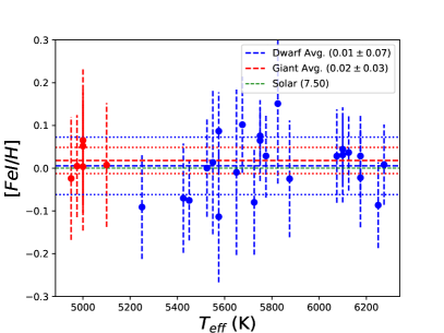
(a)

(b)

(c)

(d)

Figure 9: Individual star abundances for Iron-peak elements: Fe I, Fe II, Cr I, and Ni I. All three iron peak elements were measured at basically solar ([X/Fe]$=0.00$) levels, with no appreciable difference between the dwarf and giant populations. The abundance mean for the dwarf population is designated by the blue points and hexagon (group mean), and the giants in red.

Figure 10: Comparison of elemental abundances as measured in literature (Jofré et al.  2015) and through our process. Points are colored in red (red/pink) or blue (blue/cyan) hues to represent whether the literature value was directly measured (red) or if it was created from the literature value of [Fe/H] by assuming a solar ratio of [X/Fe] and extrapolating a “literature” [X/H] (blue). The lighter saturated colored points (pink/cyan), represent low-metallicity stars ([Fe/H] < -1.50).

References

- Allen & Porto de Mello (2011) Allen, D. M. and Porto de Mello, G. F. 2011, A&AS, 525, A63.
- Allende Prieto & Garcia Lopez (1998) Allende Prieto, C. and Garcia Lopez, R. J. 1998, A&AS, 131, 431.
- Anthony-Twarog et al. (2009) Anthony-Twarog, B. J. et al. 2009, AJ, 138, 1171.
- Arnould & Mowlavi (1995) Arnould, M. and Mowlavi, N. 1995, in Liege International Astrophysical Colloquia, volume 32 of Liege International Astrophysical Colloquia, 17.
- Asplund et al. (2009) Asplund, M. et al. 2009, ARA&A, 47, 481.
- Astropy Collaboration et al. (2013) Astropy Collaboration et al. 2013, A&A, 558, A33.
- Aurière (2003) Aurière, M. 2003, in EAS Publications Series, ed. J. Arnaud and N. Meunier, volume 9 of EAS Publications Series, 105.
- Bagnulo et al. (2003) Bagnulo, S. et al. 2003, The Messenger, 114, 10.
- Balachandran (1995) Balachandran, S. 1995, ApJ, 446, 203.
- Bard, Kock & Kock (1991) Bard, A., Kock, A., and Kock, M. 1991, A&A, 248, 315.
- Bard & Kock (1994) Bard, A. and Kock, M. 1994, A&A, 282, 1014.
- Barlow (2008) Barlow, T. 2000–2008. http://www.astro.caltech.edu/~tb/makee/.
- Bartašiūtė et al. (2007) Bartašiūtė, S. et al. 2007, Baltic Astronomy, 16, 199.
- Beveridge & Sneden (1994) Beveridge, R. C. and Sneden, C. 1994, AJ, 108, 285.
- Biazzo et al. (2007) Biazzo, K. et al. 2007, Astronomische Nachrichten, 328, 938.
- Biemont et al. (1991) Biemont, E. et al. 1991, A&A, 249, 539.
- Biemont & Godefroid (1980) Biemont, E. and Godefroid, M. 1980, A&A, 84, 361.
- Bizzarri et al. (1993) Bizzarri, A. et al. 1993, A&A, 273, 707.
- Blackwell et al. (1986) Blackwell, D. E. et al. 1986a, MNRAS, 220, 549.
- Blackwell et al. (1986) Blackwell, D. E. et al. 1986b, MNRAS, 220, 303.
- Blackwell et al. (1986) Blackwell, D. E. et al. 1986c, MNRAS, 220, 289.
- Blackwell et al. (1979) Blackwell, D. E. et al. 1979, MNRAS, 186, 633.
- Blackwell et al. (1976) Blackwell, D. E. et al. 1976, MNRAS, 177, 219.
- Blackwell, Menon & Petford (1983) Blackwell, D. E., Menon, S. L. R., and Petford, A. D. 1983, MNRAS, 204, 883.
- Blackwell, Menon & Petford (1984) Blackwell, D. E., Menon, S. L. R., and Petford, A. D. 1984, MNRAS, 207, 533.
- Blackwell et al. (1982) Blackwell, D. E. et al. 1982a, MNRAS, 201, 611.
- Blackwell, Petford & Shallis (1979) Blackwell, D. E., Petford, A. D., and Shallis, M. J. 1979, MNRAS, 186, 657.
- Blackwell et al. (1982) Blackwell, D. E. et al. 1982b, MNRAS, 199, 21.
- Blackwell et al. (1980) Blackwell, D. E. et al. 1980, MNRAS, 191, 445.
- Blackwell et al. (1982) Blackwell, D. E. et al. 1982c, MNRAS, 199, 43.
- Blackwell, Petford & Simmons (1982) Blackwell, D. E., Petford, A. D., and Simmons, G. J. 1982, MNRAS, 201, 595.
- Blackwell, Shallis & Simmons (1980) Blackwell, D. E., Shallis, M. J., and Simmons, G. J. 1980, A&A, 81, 340.
- Blanco-Cuaresma et al. (2014) Blanco-Cuaresma, S. et al. 2014a, A&A, 569, A111.
- Blanco-Cuaresma et al. (2014) Blanco-Cuaresma, S. et al. 2014b, A&A, 566, A98.
- Böcek Topcu et al. (2015) Böcek Topcu, G. et al. 2015, MNRAS, 446, 3562.
- Boesgaard, Lum & Deliyannis (2015) Boesgaard, A. M., Lum, M. G., and Deliyannis, C. P. 2015, ApJ, 799, 202.
- Boesgaard et al. (2016) Boesgaard, A. M. et al. 2016, ApJ, 830, 49.
- Boesgaard, Roper & Lum (2013) Boesgaard, A. M., Roper, B. W., and Lum, M. G. 2013, ApJ, 775, 58.
- Boesgaard & Tripicco (1986) Boesgaard, A. M. and Tripicco, M. J. 1986, ApJ, 302, L49.
- Booth et al. (1984) Booth, A. J. et al. 1984, MNRAS, 208, 147.
- Bressan et al. (2012) Bressan, A. et al. 2012, MNRAS, 427, 127.
- Buurman et al. (1986) Buurman, E. P. et al. 1986, A&A, 164, 224.
- Cardon et al. (1982) Cardon, B. L. et al. 1982, ApJ, 260, 395.
- Carraro, Monaco & Villanova (2014) Carraro, G., Monaco, L., and Villanova, S. 2014, A&A, 568, A86.
- Carrera & Pancino (2011) Carrera, R. and Pancino, E. 2011, A&A, 535, A30.
- Casagrande et al. (2010) Casagrande, L. et al. 2010, A&A, 512, A54.
- Castelli & Kurucz (2004) Castelli, F. and Kurucz, R. L. 2004, ArXiv Astrophysics e-prints.
- Castro et al. (2016) Castro, M. et al. 2016, A&A, 590, A94.
- Cohen et al. (2003) Cohen, J. G. et al. 2003, ApJ, 588, 1082.
- Cummings et al. (2017) Cummings, J. D. et al. 2017, AJ, 153, 128.
- Daniel et al. (1994) Daniel, S. et al. 1994, PASP, 106, 281.
- Den Hartog et al. (2011) Den Hartog, E. A. et al. 2011, ApJS, 194, 35.
- Den Hartog et al. (2014) Den Hartog, E. A. et al. 2014, ApJS, 215, 23.
- Donati (2003) Donati, J.-F. 2003, in Solar Polarization, ed. J. Trujillo-Bueno and J. Sanchez Almeida, volume 307 of Astronomical Society of the Pacific Conference Series, 41.
- Edvardsson et al. (1993) Edvardsson, B. et al. 1993, A&A, 275, 101.
- Francois (1988) Francois, P. 1988, A&A, 195, 226.
- Friel et al. (2002) Friel, E. D. et al. 2002, AJ, 124, 2693.
- Fry & Carney (1997) Fry, A. M. and Carney, B. W. 1997, AJ, 113, 1073.
- Fuhr, Martin & Wiese (1988) Fuhr, J. R., Martin, G. A., and Wiese, W. L. 1988, Journal of Physical and Chemical Reference Data, 17.
- Fuhrmann, Axer & Gehren (1995) Fuhrmann, K., Axer, M., and Gehren, T. 1995, A&A, 301, 492.
- Gaia Collaboration et al. (2018) Gaia Collaboration et al. 2018, ArXiv e-prints.
- Garz (1973) Garz, T. 1973, A&A, 26, 471.
- Giridhar & Arellano Ferro (1995) Giridhar, S. and Arellano Ferro, A. 1995, RMXAA, 31, 23.
- Gray & Johanson (1991) Gray, D. F. and Johanson, H. L. 1991, PASP, 103, 439.
- Hannaford et al. (1982) Hannaford, P. et al. 1982, ApJ, 261, 736.
- Hawkins et al. (2016) Hawkins, K. et al. 2016, A&A, 592, A70.
- Heinemann (1926) Heinemann, K. 1926, Astronomische Nachrichten, 227, 193.
- Heiter et al. (2015) Heiter, U. et al. 2015, A&A, 582, A49.
- Hobbs & Pilachowski (1986) Hobbs, L. M. and Pilachowski, C. 1986, ApJ, 309, L17.
- Høg et al. (2000) Høg, E. et al. 2000, A&A, 355, L27.
- Huang et al. (2015) Huang, Y. et al. 2015, MNRAS, 454, 2863.
- Iben (1991) Iben, I. 1991, APJ Suppl, 76, 55.
- Iben (1964) Iben, Jr., I. 1964, ApJ, 140, 1631.
- Jofré et al. (2015) Jofré, P. et al. 2015, A&A, 582, A81.
- Kaeppeler et al. (1990) Kaeppeler, F. et al. 1990, ApJ, 354, 630.
- Kock & Richter (1968) Kock, M. and Richter, J. 1968, ZAp, 69, 180.
- Kramida et al. (2014) Kramida, A. et al. 2014. NIST Atomic Spectra Database (ver. 5.2), [Online]. Available:http://physics.nist.gov/asd [2015, June 1].National Institute of Standards and Technology,Gaithersburg, MD.
- Kroll & Kock (1987) Kroll, S. and Kock, M. 1987, A&AS, 67, 225.
- Lambert & Luck (1978) Lambert, D. L. and Luck, R. E. 1978, MNRAS, 183, 79.
- Lambert & Warner (1968) Lambert, D. L. and Warner, B. 1968, MNRAS, 138, 213.
- Lawler & Dakin (1989) Lawler, J. E. and Dakin, J. T. 1989, Journal of the Optical Society of America B Optical Physics, 6, 1457.
- Lawler et al. (2013) Lawler, J. E. et al. 2013, ApJS, 205(2), 11.
- Lawler, Sneden & Cowan (2015) Lawler, J. E., Sneden, C., and Cowan, J. J. 2015, ApJS, 220(1), 13.
- Lawler et al. (2009) Lawler, J. E. et al. 2009, ApJS, 182, 51.
- Lawler et al. (2008) Lawler, J. E. et al. 2008, ApJS, 178(1), 71.
- Lawler et al. (2014) Lawler, J. E. et al. 2014, ApJS, 215, 20.
- Lind et al. (2011) Lind, K. et al. 2011, A&A, 528, A103.
- Maderak et al. (2013) Maderak, R. M. et al. 2013, AJ, 146, 143.
- Martin, Fuhr & Wiese (1988) Martin, G. A., Fuhr, J. R., and Wiese, W. L. 1988, Atomic transition probabilities. Scandium through Manganese, volume 17, (New York, New York: American Institute of Physics (AIP) and American Chemical Society).
- Mayor et al. (2003) Mayor, M. et al. 2003, The Messenger, 114, 20.
- McWilliam et al. (1995) McWilliam, A. et al. 1995, AJ, 109, 2757.
- McWilliam & Rich (1994) McWilliam, A. and Rich, R. M. 1994, ApJS, 91, 749.
- Meylan et al. (1993) Meylan, T. et al. 1993, ApJS, 85, 163.
- Moity (1983) Moity, J. 1983, A&AS, 52, 37.
- Nissen & Schuster (1997) Nissen, P. E. and Schuster, W. J. 1997, A&A, 326, 751.
- O’Brian et al. (1991) O’Brian, T. R. et al. 1991, Journal of the Optical Society of America B Optical Physics, 8, 1185.
- Pancino et al. (2010) Pancino, E. et al. 2010, A&A, 511, A56.
- Pavlenko et al. (2012) Pavlenko, Y. V. et al. 2012, MNRAS, 422, 542.
- Phelps, Janes & Montgomery (1994) Phelps, R. L., Janes, K. A., and Montgomery, K. A. 1994, AJ, 107, 1079.
- Pilachowski, Saha & Hobbs (1988) Pilachowski, C., Saha, A., and Hobbs, L. M. 1988, PASP, 100, 474.
- Pilachowski & Hobbs (1988) Pilachowski, C. A. and Hobbs, L. M. 1988, PASP, 100, 336.
- Platais (1991) Platais, I. 1991, A&A Suppl, 87, 69.
- Prochaska et al. (2000) Prochaska, J. X. et al. 2000, AJ, 120, 2513.
- Ramírez & Allende Prieto (2011) Ramírez, I. and Allende Prieto, C. 2011, ApJ, 743, 135.
- Ramírez & Meléndez (2005) Ramírez, I. and Meléndez, J. 2005, ApJ, 626, 465.
- Reddy, Giridhar & Lambert (2012) Reddy, A. B. S., Giridhar, S., and Lambert, D. L. 2012, MNRAS, 419, 1350.
- Reddy, Giridhar & Lambert (2013) Reddy, A. B. S., Giridhar, S., and Lambert, D. L. 2013, MNRAS, 431, 3338.
- Rentzsch-Holm (1996) Rentzsch-Holm, I. 1996, A&A, 312, 966.
- Rieke & Lebofsky (1985) Rieke, G. H. and Lebofsky, M. J. 1985, ApJ, 288, 618.
- Rohlfs & Vanysek (1962) Rohlfs, K. and Vanysek, V. 1962, Astronomische Abhandlungen der Hamburger Sternwarte, 5, 341.
- Ryabchikova et al. (2015) Ryabchikova, T. et al. 2015, Phys. Scr, 90(5).
- Salaris et al. (2015) Salaris, M. et al. 2015, A&A, 583, A87.
- Savanov, Huovelin & Tuominen (1990) Savanov, I. S., Huovelin, J., and Tuominen, I. 1990, A&AS, 86, 531.
- Schnabel, Kock & Holweger (1999) Schnabel, R., Kock, M., and Holweger, H. 1999, A&A, 342, 610.
- Sestito, Randich & Pallavicini (2004) Sestito, P., Randich, S., and Pallavicini, R. 2004, A&A, 426, 809.
- Skrutskie et al. (2006) Skrutskie, M. F. et al. 2006, AJ, 131, 1163.
- Smith & Raggett (1981) Smith, G. and Raggett, D. S. J. 1981, Journal of Physics B Atomic Molecular Physics, 14, 4015.
- Sneden (1973) Sneden, C. 1973, ApJ, 184, 839.
- Sneden et al. (2012) Sneden, C. et al. 2012. Astrophysics Source Code Library.
- Sneden et al. (2014) Sneden, C. et al. 2014, ApJS, 214, 26.
- Sobeck, Lawler & Sneden (2007) Sobeck, J. S., Lawler, J. E., and Sneden, C. 2007, ApJ, 667(2), 1267.
- Space Telescope Science Institute (2014) Space Telescope Science Institute 1990–2014. http://www.stsci.edu/institute/software_hardware/stsdas.
- Stephens (1999) Stephens, A. 1999, AJ, 117, 1771.
- Stetson & Pancino (2008) Stetson, P. B. and Pancino, E. 2008, PASP, 120, 1332.
- Takeda (2003) Takeda, Y. 2003, A&A, 402, 343.
- Takeda, Ohkubo & Sadakane (2002) Takeda, Y., Ohkubo, M., and Sadakane, K. 2002, PASJ, 54, 451.
- Twarog et al. (2015) Twarog, B. A. et al. 2015, AJ, 150, 134.
- Ventura, Carini & D’Antona (2011) Ventura, P., Carini, R., and D’Antona, F. 2011, MNRAS, 415, 3865.
- Vogt et al. (1994) Vogt, S. S. et al. 1994, in Instrumentation in Astronomy VIII, ed. D. L. Crawford and E. R. Craine, volume 2198 of Proc. SPIE, 362.
- Wallace et al. (2011) Wallace, L. et al. 2011, ApJS, 195, 6.
- Wenger et al. (2000) Wenger, M. et al. 2000, A&AS, 143, 9.
- Wickliffe & Lawler (1997) Wickliffe, M. E. and Lawler, J. E. 1997, ApJS, 110, 163.
- Wiese & Martin (1980) Wiese, W. L. and Martin, G. A. 1980, Wavelengths and transition probabilities for atoms and atomic ions: Part 2. Transition probabilities, NSRDS-NBS Vol. 68., (Washington D.C.: NSRDS-NBS, US Department of Commerce, National Bureau of Standards).
- Wood et al. (2013) Wood, M. P. et al. 2013, The Astrophysical Journal Supplement Series, 208(2), 27.
- Wood et al. (2014) Wood, M. P. et al. 2014, The Astrophysical Journal Supplement Series, 211(2), 20.