Scaling limits for random triangulations on the torus

Abstract

We study the scaling limit of essentially simple triangulations on the torus. We consider, for every $n\geq 1$, a uniformly random triangulation $G_{n}$ over the set of (appropriately rooted) essentially simple triangulations on the torus with $n$ vertices. We view $G_{n}$ as a metric space by endowing its set of vertices with the graph distance denoted by $d_{G_{n}}$ and show that the random metric space $(V(G_{n}),n^{-1/4}d_{G_{n}})$ converges in distribution in the Gromov–Hausdorff sense when $n$ goes to infinity, at least along subsequences, toward a random metric space. One of the crucial steps in the argument is to construct a simple labeling on the map and show its convergence to an explicit scaling limit. We moreover show that this labeling approximates the distance to the root up to a uniform correction of order $o(n^{1/4})$.

Keywords: random maps, unicellular maps, Schnyder woods, toroidal triangulations

1 Introduction

1.1 Some definitions

Recall that the Hausdorff distance between two non-empty subsets $X$ and $Y$ of a metric space $(M,d)$ is defined as

$$d_{Haus}(X,Y)=\inf\{\epsilon\geq 0:X\subset Y_{\epsilon}\quad\textrm{and}\quad Y\subset X_{\epsilon}\},$$

where $Z_{\epsilon}$ denotes $\{m\in M:d(m,Z)\leq\epsilon\}$. The Gromov-Hausdorff distance between two compact metric spaces $(S,\delta)$ and $(S^{\prime},\delta^{\prime})$ is defined as

$$d_{GH}((S,\delta),(S^{\prime},\delta^{\prime}))=\inf\{d_{Haus}(\varphi(S),\varphi^{\prime}(S^{\prime})\},$$

where the infimum is taken over all isometric embeddings $\varphi:S\rightarrow S"$ and $\varphi^{\prime}:S^{\prime}\rightarrow S"$ of $S$ and $S^{\prime}$ into a common metric space $(S",\delta")$. Note that $d_{GH}((S,\delta),(S^{\prime},\delta^{\prime}))$ is equal to $0$ if and only if the metric spaces $S$ and $S^{\prime}$ are isometric to each other. We refer the reader to e.g. [1, Section 3] for a detailed investigation of the Gromov-Hausdorff distance.

In this paper, we are considering some random graphs seen as random metric spaces and consider their convergence in distribution in the sense of the Gromov-Hausdorff distance. In general, graphs may contain loops and multiple edges. A graph is called simple if it contains no loop nor multiple edges. A graph embedded on a surface is called a map on this surface if all its faces are homeomorphic to open disks. In this paper we consider orientable surface of genus $g$ where the plane is the surface of genus $0$, the torus the surface of genus $1$, etc. For $p\geq 3$, a map is called a $p$-angulation if all its faces have size $p$. For $p=3$ (resp. $p=4$), such maps are respectively called triangulations (resp. quadrangulations).

1.2 Random planar maps

Let us first review some results on random planar maps. Consider a random planar map $G_{n}$ with $n$ vertices which is uniformly distributed over a certain class of planar maps (like planar triangulations, quadrangulations or $p$-angulations). Equip the vertex set $V(G_{n})$ with the graph distance $d_{G_{n}}$. It is known that the diameter of the resulting metric space is of order $n^{1/4}$ (see for example [10] for the case of quadrangulations). Thus one can expect that the rescaled random metric spaces $(V(G_{n}),n^{-1/4}d_{G_{n}})$ converge in distribution as $n$ tends to infinity toward a certain random metric space. In 2006, Schramm [25] suggested to use the notion of Gromov-Hausdorff distance to formalize this question by specifying the topology of this convergence. He was the first to conjecture the existence of a scaling limit for large random planar triangulations. In 2011, Le Gall [17] proved the existence of the scaling limit of the rescaled random metric spaces $(V(G_{n}),n^{-1/4}d_{G_{n}})$ for $p$-angulations when $p=3$, or, $p\geq 4$ and $p$ is even. The case $p=3$ solves the conjecture of Schramm. Miermont [19] gave an alternative proof in the case of quadrangulations $(p=4)$. Addario-Berry and Albenque [1] prove the case $p=3$ for simple triangulations (i.e. triangulations with no loop nor multiple edges). An important aspect of all these results is that, up to a constant rescaling factor, all these classes converge toward the same object called the Brownian map.

It is natural to address the question of the existence of a scaling limit of random maps on higher genus oriented surfaces. Chapuy, Marcus and Schaeffer [9] extended the bijection known for planar bipartite quadrangulations to any oriented surfaces. This led Bettinelli [4] to show that random quadrangulations on oriented surfaces converge in distribution, at least along a subsequence. More formally:

Theorem 1 (Bettinelli [4]).

For $g\geq 1$ and $n\geq 1$, let $G_{n}$ be a uniformly random element of the set of all angle-rooted bipartite quadrangulations with $n$ vertices on the oriented surface of genus $g$. Then, from any increasing sequence of integers, one can extract a subsequence $(n_{k})_{k\geq 0}$ along which the rescaled metric spaces

$$\left(V(G_{n_{k}}),n_{k}^{-1/4}d_{G_{n_{k}}}\right)_{k\geq 0}$$

converge in distribution for the Gromov-Hausdorff distance.

Contrary to the planar case, the uniqueness of the subsequential limit is not proved there. Nevertheless, a phenomenon of universality is expected: it is conjectured that the sequence does converge and that moreover, up to a deterministic multiplicative constant on the distance, the limit is the same for many models of random maps of a given genus. In genus $1$, the conjectured limit is described in [4] and referred to as the toroidal Brownian map.

The present article extends Theorem 1 to the case of (essentially simple) triangulations of the torus. In that respect, it is comparable to the paper of Addario-Berry and Albenque [1] which did the same in the planar setup and thus our work contributes to the understanding of universality for random toroidal maps.

1.3 Main results

A contractible loop is an edge enclosing a region homeomorphic to an open disk. A pair of homotopic multiple edges is a pair of edges that have the same extremities and whose union encloses a region homeomorphic to an open disk. A graph $G$ embedded on the torus is called essentially simple if it has no contractible loop nor homotopic multiple edges. Being essentially simple for a toroidal map is the natural generalization of being simple for a planar map.

In this paper, we distinguish paths and cycles from walks and closed walks as the firsts have no repeated vertices. A triangle of a toroidal map is a closed walk of size $3$ enclosing a region that is homeomorphic to an open disk. This region is called the interior of the triangle. Note that a triangle is not necessarily a face of the map as its interior may be not empty. We say that a triangle is maximal (by inclusion) if its interior is not strictly contained in the interior of another triangle. We define the corners of a triangle as the three angles that appear in the interior of this triangle when its interior is removed (if non empty).

Our main result is the following convergence result:

Theorem 2.

For $n\geq 1$, let $G_{n}$ be a uniformly random element of the set of all essentially simple toroidal triangulations on $n$ vertices that are rooted at a corner of a maximal triangle. Then, from any increasing sequence of integers, one can extract a subsequence $(n_{k})_{k\geq 0}$ along which the rescaled metric spaces

$$\left(V(G_{n_{k}}),n_{k}^{-1/4}d_{G_{n_{k}}}\right)_{k\geq 0}$$

converge in distribution for the Gromov-Hausdorff distance.

Remark 1.

The reason for the particular choice of rooting in Theorem 2 is of a technical nature due to the bijection that we use in Section 2. It is a natural conjecture that compactness, and thus also the existence of subsequential scaling limits, would still hold e.g. for triangulations rooted at a uniformly random angle. This is based on the following reasoning: if the inside of every maximal triangle has diameter of smaller order than $n^{1/4}$, then rooting inside such a triangle rather than at one of its corners would affect distances by a quantity that would be smoothed out by the normalization. On the other hand, having one maximal triangle containing $\alpha n$ vertices has very small probability, because of the relative growths of the number of triangulations of genus $0$ and $1$. The remaining obstruction would be the existence of a maximal triangle with an inside containing much fewer than $n$ vertices but having diameter of order $n^{1/4}$, which would presumably be ruled out by a precise control of the geometry of simple triangulations of genus $0$. This is a possible direction for future work, but we chose not to investigate it further due to the already large size of the present paper.

We also show in an appendix that with high probability, the labeling function that we define as a crucial tool in our argument (see Section 3 for a formal definition) approximates the distance to the root up to a uniform $o(n^{1/4})$ correction (see Theorem 5). Such a comparison estimate is an essential step in proving the uniqueness of the subsequential scaling limit, and thus the convergence, in frameworks similar to that of our main result — see [1] for the case of genus $0$, it is also likely that a similar argument would be applicable to quadrangulations of the torus [5] (those two quantities are actually equal in the case of bipartite quadrangulations on any surface with positive genus, but it seems that a bound of the order $o(n^{1/4})$ is enough).

The overall strategy for the proof of Theorem 2 is the same as in [4], as well as in [17] and [19]: obtain a bijection between maps and simpler combinatorial objects (typically decorated trees), then show the convergence of these objects to a non-trivial continuous random limit from which relevant information can then be extracted about the original model. As a result, most of the structure of the paper is largely inspired by [4] (for the main argument) and [1] (for methods specific to triangulations).

The bijection that we use here is based on a recent generalization of Schnyder woods to higher genus [15, 14, 18]. One issue when going to higher genus is that the set of Schnyder woods of a given triangulation is no longer a single distributive lattice like in the planar case, it is rather a collection of distributive lattices. Nevertheless, it is possible to single out one of these distributive lattices, in the toroidal case, by requiring an extra property, called balanced, that defines a unique minimal element used as a canonical orientation for the toroidal triangulation. The particular properties of this canonical orientation leads to a bijection between essentially simple toroidal triangulation and particular toroidal unicellular maps [12] (a unicellular map is a map with only one face, i.e. the natural generalization of trees when going to higher genus). Then the main difficulty that we have to face is that the metric properties of the initial map are less apparent in the unicellular map than in the planar case or in the bipartite quadrangulations setup.

Structure of the paper

The bijection between toroidal triangulations and particular unicellular maps is presented in Section 2 with some related properties. In Section 3, we define a labeling function of the angles of a unicellular map and prove some relations with the graph distance in the corresponding triangulation. In Section 4 we explain how to decompose the particular unicellular maps given by the bijection into simpler elements with the use of Motzkin paths and well-labeled forests. In Section 5, we review some results on variants of the Brownian motion. Then the proof of Theorem 2 then proceeds in several steps. In Section 6, we study the convergence of the parameters of the discrete map in the scaling limit. In Sections 7, 8 and 9 we review and extend classical convergence results for conditioned random walks and random forests. Finally, in Section 10, we combine the previous ingredients to build the proof of the main theorem. In Appendix A, we exploit the canonical orientation of the triangulation to define rightmost paths and relate them to shortest paths, thus obtaining the announced upper bound on the difference between distances and labels.

This work has been partially supported by the LabEx PERSYVAL-Lab (ANR-11-LABX-0025-01) funded by the French program Investissement d’avenir and the ANR project GATO (ANR-16-CE40-0009-01) funded by the French Agence National de la Recherche.

2 Bijection between toroidal triangulations and unicellular maps

For $n\geq 1$, let $\mathcal{G}(n)$ be the set of essentially simple toroidal triangulations on $n$ vertices that are rooted at a corner of a maximal triangle.

Consider an element $G$ of $\mathcal{G}(n)$. The corner of the maximal triangle where $G$ is rooted is called the root corner. Note that, since $G$ is essentially simple, there is a unique triangle, called the root triangle, whose corner is the root corner (and this root triangle is maximal by assumption). The vertex of the root triangle corresponding to the root corner is called the root vertex. We also define, in a unique way, a particular angle of the map, called the root angle, that is the angle of $G$ that is in the interior of the root triangle, incident to the root vertex and the last one in counterclockwise order around the root vertex. Note that it is possible to retrieve the root corner from the root angle in a unique way (indeed, the root angle defines already one edge of the root triangle and the side of its interior, thus it remains to find the third vertex of the root triangle such that the interior is maximal). Thus rooting $G$ on its root corner or root angle is equivalent. We call root face, the face of $G$ containing the root angle. We introduce in the rest of this section some terminology and results adapted from [12] (see also [18]).

2.1 Toroidal unicellular maps

Recall that a unicellular map is a map with only one face. There are two types of toroidal unicellular maps since two cycles of a toroidal unicellular map may intersect either on a single vertex (square case) or on a path (hexagonal case). On the first row of Figure 1 we have represented these two cases into a square box that is often use to represent a toroidal object (its opposite sides are identified). On the second row of Figure 1 we have represented again these two cases by a square and hexagon by copying some vertices and edges of the map (here again the opposite sides are identified). Depending on what we want to look at we often move from one representation to the other in this paper. We call special the vertices of a toroidal unicellular map that are on all the cycles of the map. Thus the number of special vertices of a square (resp. hexagon) toroidal unicellular map is exactly one (resp. two).

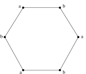
Square case	Hexagonal case

Figure 1: The two types of toroidal unicellular maps with two different representations for each case.

Given a map, we call stem, a half-edge that is added to the map, attached to an angle of a vertex and whose other extremity is dangling in the face incident to this angle.

For $n\geq 1$, let $\mathcal{T}_{r}(n)$ denote the set of toroidal unicellular maps rooted on a particular angle, with exactly $n$ vertices, $n+1$ edges and $2n-1$ stems distributed as follows (see figure 2 for an example in $\mathcal{T}_{r}(7)$ where the root angle is represented with the usual "root" symbol in the whole paper.). The vertex incident to the root angle is called the root vertex. A vertex that is not the root vertex, is incident to exactly $2$ stems if it is not a special vertex, $1$ stem if it is the special vertex of a hexagon and $0$ stem if it is the special vertex of a square. The root vertex is incident to $1$ additional stem, i.e. it is incident to exactly $3$ stems if it is not a special vertex, $2$ stems if it is the special vertex of a hexagon and $1$ stem if it is the special vertex of a square. Moreover, one of the stem incident to the root vertex, called the root stem, is incident to the root angle and just after the root angle in counterclockwise order around the root vertex.

Figure 2: Example of an element of $\mathcal{T}_{r}(7)$.

2.2 Closure procedure

Given an element $T$ of $\mathcal{T}_{r}(n)$, there is a generic way to attach step by step all the dangling extremities of the stems of $T$ to build a toroidal triangulation. Let $T_{0}=T$, and, for $1\leq k\leq 2n-1$, let $T_{k}$ be the map obtained from $T_{k-1}$ by attaching the extremity of a stem to an angle of the map (we explicit below which stems can be attached and how). The special face of $T_{0}$ is its only face. For $1\leq k\leq 2n-1$, the special face of $T_{k}$ is the face on the right of the stem of $T_{k-1}$ that is attached to obtain $T_{k}$ (the stem is by convention oriented from its incident vertex toward its dangling part). For $0\leq k\leq 2n-1$, the border of the special face of $T_{k}$ consists of a sequence of edges and stems. We define an admissible triple as a sequence $(e_{1},e_{2},s)$, appearing in counterclockwise order along the border of the special face of $T_{k}$, such that $e_{1}=(u,v)$ and $e_{2}=(v,w)$ are edges of $T_{k}$ and $s$ is a stem attached to $w$. The closure of this admissible triple consists in attaching $s$ to $u$, so that it creates an edge $(w,u)$ oriented from $w$ to $u$ and so that it creates a triangular face $(u,v,w)$ on its left side. The complete closure of $T$ consists in closing a sequence of admissible triples, i.e. for $1\leq k\leq 2n-1$, the map $T_{k}$ is obtained from $T_{k-1}$ by closing any admissible triple.

Figure 3 is the hexagonal representation of the example of Figure 2 on which a complete closure is performed. We have represented here the unicellular map as an hexagon since it is easier to understand what happen in the unique face of the map. The map obtained by performing the complete closure procedure is the clique on seven vertices $K_{7}$.

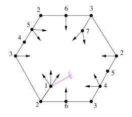
A unicellular map of $\mathcal{T}_{r,s,b}(7)$	The complete closure gives $K_{7}$

Figure 3: Example of the complete closure procedure.

Note that, for $0\leq k\leq 2n-1$, the special face of $T_{k}$ contains all the stems of $T_{k}$. The closure of a stem reduces the number of edges on the border of the special face and the number of stems by $1$. At the beginning, the unicellular map $T_{0}$ has $n+1$ edges and $2n-1$ stems. So along the border of its special face, there are $2n+2$ edges and $2n-1$ stems. Thus there is exactly three more edges than stems on the border of the special face of $T_{0}$ and this is preserved while closing stems. So at each step there is necessarily at least one admissible triple and the sequence $T_{k}$ is well defined. Since the difference of three is preserved, the special face of $T_{2n-2}$ is a quadrangle with exactly one stem. So the attachment of the last stem creates two faces that have size three and at the end $T_{2n-1}$ is a toroidal triangulation. Note that at a given step there might be several admissible triples but their closure are independent and the order in which they are closed does not modify the obtained triangulation $T_{2n-1}$.

When a stem is attached on the root angle, then, by convention, the new root angle is maintained on the right side of the extremity of the stem, i.e. the root angle is maintained in the special face. A particularly important property when attaching stems is when the complete closure procedure described here never wraps over the root angle, i.e. when a stem is attached, the root angle is always on its right side in the special face. The property of never wrapping over the root angle is called safe (an analogous property is sometimes called "balanced" in the planar case but we prefer to keep the word "balanced" for something else in the current paper). Let $\mathcal{T}_{r,s}(n)$ denote the set of elements of $\mathcal{T}_{r}(n)$ that are safe.

Consider an element $T$ of $\mathcal{T}_{r,s}(n)$ with root angle $a_{0}$. Then for $0\leq k\leq 2n-2$, let $s$ be the first stem met while walking counterclockwise from $a_{0}$ in the special face of $T_{k}$. An essential property from [12] is that before $s$, at least two edges are met and thus the last two of these edges form an admissible triple with $s$. So one can attach all the stems of $T$ by starting from the root angle $a_{0}$ and walking along the face of $T$ in counterclockwise order around this face: each time a stem is met, it is attached in order to create a triangular face on its left side. Note that in such a sequence of admissible triples closure, the last stem that is attached is the root stem of $T$.

2.3 Canonical orientation and balanced property

For $n\geq 1$, consider an element $T$ of $\mathcal{T}_{r}(n)$ whose edges and stems are oriented w.r.t. the root angle $a_{0}$ as follows (see Figure 4 that corresponds to the example of Figure 2): the stems are all outgoing, and while walking clockwise around the unique face of $T$ from $a_{0}$, the first time an edge is met, it is oriented counterclockwise w.r.t. the face of $T$. This orientation plays a particular role and is called the canonical orientation of $T$.

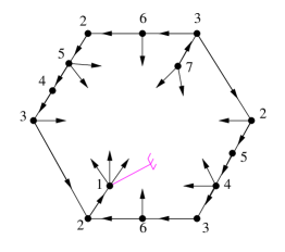
Figure 4: Orientation of the edges and stems of an element of $\mathcal{T}_{r}(7)$.

For a cycle $C$ of $T$, given with a traversal direction, let $\gamma(C)$ be the number of outgoing edges and stems that are incident to the right side of $T$ minus the number of outgoing edges and stems that are incident to its left side. A unicellular map of $\mathcal{T}_{r}(n)$ is said to be balanced if $\gamma(C)=0$ for all its (non-contractible) cycles $C$. Let us call $\mathcal{T}_{r,s,b}(n)$ the set of balanced elements of $\mathcal{T}_{r,s}(n)$.

Figure 4 is an example of an element of $\mathcal{T}_{r,s,b}(7)$. The values $\gamma$ of the cycles of the unicellular map are much more easier to compute on the left representation.

A consequence of [12] (see the proof of Theorem 7 where $\mathcal{T}_{r,s,b}(n)$ is called $\mathcal{U}^{\prime}_{r,b,\gamma_{0}}(n)$ and $\mathcal{G}(n)$ is called $\mathcal{T}^{\prime}_{r}(n)$), is that, for $n\geq 1$, the complete closure procedure is indeed a bijection between elements of $\mathcal{T}_{r,s,b}(n)$ and $\mathcal{G}(n)$, that we denote $\Phi$ in the curent paper:

Theorem 3 ([12]).

For $n\geq 1$, there is a bijection between $\mathcal{T}_{r,s,b}(n)$ and $\mathcal{G}(n)$.

The left of Figure 3 gives an example of a hexagonal unicellular map in $\mathcal{T}_{r,s,b}(7)$. Note that on the right of Figure 3, the face containing the root angle, after the closure procedure, is indeed a maximal triangle, so the obtained triangulation is an element of $\mathcal{G}(7)$ if rooted on the corner of the face corresponding to the root angle.

Given an element $T$ of $\mathcal{T}_{r,s,b}(n)$, the canonical orientation of $T$, defined previously, induces an orientation of the edges of the corresponding triangulation $G$ of $\mathcal{G}(n)$ that is also called the canonical orientation of $G$. Note that in this orientation of $G$, all the vertices have outdegree exactly $3$, we call such an orientation a $3$-orientation. In fact this orientation corresponds to a particular $3$-orientation that is called the minimal balanced Schnyder wood of $G$ w.r.t. to the root face (see [18] for more on Schnyder woods in higher genus). We extend the definition of function $\gamma$ to $G$ by the following. For a cycle $C$ of $G$, given with a traversal direction, let $\gamma(C)$ be the number of outgoing edges that are incident to the right side of $T$ minus the number of outgoing edges that are incident to its left side. As shown in [18], the canonical orientation of $G$ as the particular property that $\gamma(C)=0$ for all its non-contractible cycles $C$, we call this property balanced.

Figure 5, gives the canonical orientation of $K_{7}$ obtained from the canonical orientation of its corresponding element in $\mathcal{T}_{r,s,b}(7)$ after a complete closure procedure.

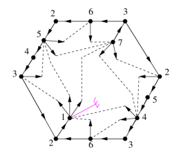
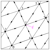
Figure 5: The canonical orientation of $K_{7}$.

2.4 Unrooted unicellular maps

Given an element $T$ of $\mathcal{T}_{r,s,b}(n)$, we have seen that the root stem $s_{0}$ can be the last stem that is attached by the complete closure procedure. Consequently, if one removes the root stem $s_{0}$ from $T$ to obtain an unicellular map $U$ with $n$ vertices, $n+1$ edges and $2n-2$ stems, one can recover the graph $T_{2n-2}$ by applying the closure procedure on $U$.

For $n\geq 1$, let $\mathcal{U}(n)$ denote the set of (non-rooted) toroidal unicellular maps, with exactly $n$ vertices, $n+1$ edges and $2n-2$ stems satisfying the following: a vertex is incident to exactly $2$ stems if it is not a special vertex, $1$ stem if it is the special vertex of a hexagon and $0$ stem if it is the special vertex of a square. Thus, given an element $T$ of $\mathcal{T}_{r}(n)$, the element $U$ obtained from $T$ by removing the root angle and the root stem is an element of $\mathcal{U}(n)$.

Since an element $U$ of $\mathcal{U}(n)$ is non-rooted, it has no "canonical orientation" as define previously for elements of $\mathcal{T}_{r}(n)$. Nevertheless one can still orient all the stems as outgoing and compute $\gamma$ on the cycles of $U$ by considering only its stems in the counting (and not the edges nor the root stem anymore). For a cycle $C$ of $U$, given with a traversal direction, let $\gamma(C)$ be the number of outgoing stems that are incident to the right side of $U$ minus the number of outgoing stems that are incident to its left side. A unicellular map of $\mathcal{U}(n)$ is said to be balanced if $\gamma(C)=0$ for all its (non-contractible) cycles $C$. Let us call $\mathcal{U}_{b}(n)$ the set of elements of $\mathcal{U}(n)$ that are balanced.

As remarked in [12], an interesting property is that an element $U$ of $\mathcal{U}(n)$ is balanced if and only if any element $T$ of $\mathcal{T}_{r}(n)$ obtained from $U$ by adding a root stem anywhere in $U$ is balanced (recall that in $U$ we use the canonical orientation to compute $\gamma$). Moreover, given an element $T$ of $\mathcal{T}_{r,b}(n)$, then the element $U$ of $\mathcal{U}(n)$, obtained by removing the root angle, (the canonical orientation,) and the root stem is balanced.

Figure 6 is the element of $\mathcal{U}_{b}(7)$ corresponding to Figure 4.

Figure 6: Example of an element of $\mathcal{U}_{b}(7)$.

3 Labeling of the angles and distance properties

For $n\geq 1$, let $T$ be an element of $\mathcal{T}_{r,s,b}(n)$, and $G=\Phi(T)$ the corresponding element of $\mathcal{G}(n)$ by Theorem 3. Let $V$ (resp. $E$) denotes the set of vertices (resp. edges) of $G$. Let $a_{0}$ be the root angle of $T$ and $v_{0}$ be its root vertex. We use the same notations for the root angle and vertex of $G$ (while maintaining the root angle on the right side of every stem during the complete closure procedure, as explained in Section 2). In this section, we prove some relations between the graph distance in the triangulation $G$ and a particular labeling of the vertices defined on the unicellular map $T$.

3.1 Definition and properties of the labeling function

Let $\ell=4n+1$ be the number of angles of $T$. We add a special dangling half-edge incident to the root angle of $T$, called the root half-edge (and not considered as a stem). Let $\Gamma$ be the obtained unicellular map. We define the root angle of $\Gamma$ as the angle of $\Gamma$ just after the root half-edge in counterclockwise order around its incident vertex. Let $A=(a_{0},\ldots,a_{\ell})$ be the sequence of consecutive angles of $\Gamma$ in clockwise order around the unique face of $\Gamma$ such that $a_{0}$ is the root angle. Note that $a_{\ell}$ is incident to the root half-edge. For $0\leq i\leq l-1$, two angles $a_{i}$ and $a_{i+1}$ are either consecutive around a stem or consecutive around an edge of $\Gamma$. We define a labeling function $\lambda:A\rightarrow\mathbb{Z}$ as follows. Let $\lambda(a_{0})=3$. For $0\leq i\leq l-1$, let $\lambda(a_{i+1})=\lambda(a_{i})+1$ if $a_{i}$ and $a_{i+1}$ are consecutive around a stem, and let $\lambda(a_{i+1})=\lambda(a_{i})-1$ if they are consecutive around an edge. By definition, the unicellular map $\Gamma$ has $n+1$ edges and $2n-1$ stems. While going clockwise around the unique face of $\Gamma$, each edge is encountered twice, so $\lambda(a_{\ell})=2n-1-2(n+1)+\lambda(a_{0})=0$. Figure 7 gives an example of the labeling function of the unicellular map of Figure 4.

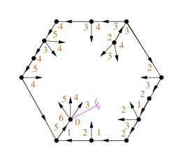
Figure 7: Labeling of the angles of the unicellular map.

Given a stem $s$ of $\Gamma$, we define the label $\lambda(s)$ of $s$ as the label of the angle that is just before $s$ in counterclockwise order around its incident vertex.

The complete closure procedure is formally defined on $T$ but we can consider that it behaves on $\Gamma$ since the presence of the root half-edge in $\Gamma$ does not change the procedure as $T$ is safe (the root half-edge is maintained on the right of every stem during the closure). Let $\Gamma_{0}=\Gamma$, and, for $1\leq k\leq 2n-1$, let $\Gamma_{k}$ be the map obtained from $\Gamma_{k-1}$ by closing an admissible triple of $\Gamma_{k-1}$. By the bijection $\Phi$ we have that $\Gamma_{2n-1}$ is the graph $G$ with an additional dangling half-edge incident to the root angle, we call this graph $G^{+}$. We propagate the labeling $\lambda$ of $\Gamma$ during the closure procedure by the following. For $1\leq k\leq 2n-1$, when the stem $s$ of $\Gamma_{k-1}$ is attached, it splits an angle $a$ of $\Gamma_{k-1}$ into two angles of $\Gamma_{k}$ that both inherit the label of $a$ in $\Gamma_{k-1}$. In other words, the complete closure procedure just splits some angles that keeps the same label on each side of the split. We still note $\lambda$ the labeling of the angles of $\Gamma_{k}$. It is clear that the labeling of $G^{+}=\Gamma_{2n-1}$ that is obtained is independent from the order in which the admissible triples are closed. We denote $\mathcal{A}(i)$ the set of angles of $G^{+}$ which are splited from $a_{i}$ by the complete closure procedure. Note that for all $a\in\mathcal{A}(i)$, we have $\lambda(a)=\lambda(a_{i})$. Given a stem $s$ of $\Gamma$, we denote $a(s)$ the angle of $\Gamma$ corresponding to where $s$ is attached during the complete closure procedure (i.e. $s$ is attached to an angle that comes from some splittings of $a(s)$).

Consider a stem $s$ of $T$. Let $i,j$, be such that $a_{i}$ is the angle just before $s$ in counterclockwise order around its incident vertex and $a_{j}=a(s)$. The fact that $T$ is safe implies that $0\leq i<j\leq\ell$.

Lemma 1.

For $0\leq k\leq 2n-1$, the rules that are used to define the labeling function $\lambda$ are still valid around the special face of $\Gamma_{k}$, i.e. the root angle of $\Gamma_{k}$ is labeled $3$, and while walking clockwise around the special face of $\Gamma_{k}$, the labels are increasing by one around a stem and decreasing by one along an edge until finishing at label $0$ at the last angle.

In particular, for each stem $s$ of $\Gamma$, we have $\lambda(a(s))=\lambda(s)-1$. Moreover, all the angles of $\Gamma$ that appear strictly between $s$ and $a(s)$ in clockwise order along the unique face of $\Gamma$ have labels that are greater or equal to $\lambda(s)$.

Proof.

We prove the first part of the lemma by induction on $k$. Clearly the statement is true for $k=0$ by definition and properties of $\lambda$. Suppose now that for $1\leq k\leq 2n-1$, the statement is true for $\Gamma_{k-1}$. Let $s$ be the stem of $\Gamma_{k-1}$ that is attached to obtained $\Gamma_{k}$. Let $(e_{1},e_{2},s)$ be the admissible triple of $\Gamma_{k-1}$ involving $s$, when $s$ is attached. Let $\alpha_{0},\alpha_{1},\alpha_{2},\alpha_{3}$ be the angles of the special face of $\Gamma_{k-1}$ that appears along the admissible triple $(e_{1},e_{2},s)$, such that $\alpha_{0},s,\alpha_{1},e_{1},\alpha_{2},e_{2},\alpha_{3}$ appears consecutively in clockwise order around the special face. So we have that the dangling part of $s$ is attached to the angle $\alpha_{3}$ to form $\Gamma_{k}$. Since $T$ is safe, the root angle of $\Gamma_{k-1}$ is distinct from $\alpha_{1},\alpha_{2},\alpha_{3}$. So, by induction, the rules of the labeling function applies in $\Gamma_{k-1}$ from $\alpha_{0}$ to $\alpha_{3}$. Thus $\lambda(\alpha_{1})=\lambda(\alpha_{0})+1$, $\lambda(\alpha_{2})=\lambda(\alpha_{1})-1$, $\lambda(\alpha_{3})=\lambda(\alpha_{2})-1$. So $\lambda(\alpha_{3})=\lambda(\alpha_{1})-1$, and the rules still apply in the special face of $\Gamma_{k}$.

A direct consequence of the above paragraph, is that for each stem $s$ of $\Gamma$, we have $\lambda(a(s))=\lambda(s)-1$.

Suppose by contradiction that there is a stem $s$ and an angle of $\Gamma$ that appear strictly between $s$ and $a(s)$ in clockwise order along the unique face of $\Gamma$ whose label is less or equal to $\lambda(a(s))$. We choose such an angle $\alpha$ whose label is minimum. With the same notations of the angles $\alpha_{1},\alpha_{2}$ as above, since $\lambda(\alpha_{2})=\lambda(a(s))+1$ and $\lambda(\alpha_{1})=\lambda(a(s))+2$, we have that neither $\alpha_{1}$ nor $\alpha_{2}$ comes from a splits of $\alpha$. So there exists an admissible triple $s^{\prime}$, closed before $s$ is the complete closure procedure, and whose one of the two internal angles $\alpha^{\prime}_{1},\alpha^{\prime}_{2}$ (with analogous notations as above) is $\alpha$ (or comes from a split of $\alpha$). By the rule of the labeling, we have $\lambda(\alpha)\in\{\lambda(a(s^{\prime}))+1,\lambda(a(s^{\prime}))+2\}$ (depending on which internal angle it is, either $\alpha^{\prime}_{1}$ or $\alpha^{\prime}_{2}$). Thus by minimality of $\alpha$, we have $a(s^{\prime})=a(s)$, but then $\lambda(\alpha)\in\{\lambda(a(s))+1,\lambda(a(s))+2\}$, a contradiction. ∎

Lemma 2.

Consider a (non-contractible) cycle $C$ of $\Gamma$ of length $k$ that does not contain the root vertex. Then there is exactly $k-1$ stems attached to each side of $C$.

Proof.

As explained in Section 2.4, when one remove from $T$ the root stem, the canonical orientation and the root angle, one obtain an element of $\mathcal{U}_{b}(n)$. So we have that the number of stems attached to the left and right side of $C$ are the same. In both cases, whether $\Gamma$ is a square or hexagonal unicellular map, we have that $C$ is incident to exactly $2(k-1)$ stems, so there is exactly $k-1$ stems attached to each side of $C$. ∎

Note that if $v_{0}\in C$ then the conclusion of Lemma 2 is not true since there is an additional stem attached to the root vertex.

Lemma 3.

For $0\leq i\leq\ell-1$, we have $\lambda(a_{i})>0$.

Proof.

Assume that there exists $0\leq i\leq\ell-1$, such that $\lambda(a_{i})\leq 0$. Let $k=\max\left\{0\leq i\leq l-1:\lambda(a_{i})\leq 0\right\}$. If $a_{k}$ and $a_{k+1}$ are consecutive along an edge, then we have $\lambda(a_{k+1})=\lambda(a_{k})-1<0$. If $a_{k}$ and $a_{k+1}$ are separated by a stem, then, by Lemma 1, we have $\lambda(a(s))=\lambda(a_{k})-1$ , so there exists $k^{\prime}>k$ such that $\lambda(a_{k^{\prime}})<0$. In both cases, there is a contradiction to the definition of $k$. ∎

Let $V_{S}$ be the set of special vertices of $\Gamma$ (defined in Section 2). We call proper the edges and vertices of $\Gamma$ that are on at least one cycle of $\Gamma$. Let $V_{P}$ (respectively $E_{P}$) be the set of proper vertices (respectively edges) of $\Gamma$. Note that $V_{S}\subseteq V_{P}$.

We call root path the (unique) shortest path of $\Gamma$ from the root vertex to a proper vertex. Note that the root path might have length $0$ if $v_{0}$ is proper. The sequence of vertices along the root path is denoted $V_{R}=(r_{0},r_{1},...,r_{s})$, with $s\geq 0$, $r_{0}=v_{0}$ and $r_{s}$ is proper. The set of edges of the root path is denoted $E_{R}$. Let $V_{N}=V\setminus(V_{P}\bigcup V_{R})$ be the set of normal vertices of $\Gamma$ and $E_{N}=E\setminus(E_{P}\bigcup E_{R})$ be the set of normal edges of $\Gamma$.

The canonical orientation of $\Gamma$ is the orientation of the edges and stems of $\Gamma$ that corresponds to the canonical orientation of $T$ (the root half edge added has no particular orientation). Consider an edge $e$ of $\Gamma$ with its orientation in the canonical orientation, then by the orientation rule, the angles of $\gamma$ incident to $e$ that are on its right side have greater indices in the set $A$ than the angles that are on its left side, i.e. they are seen after while going in clockwise order around the unique face of $\Gamma$ starting from the root angle.

Lemma 4.

Consider an edge $e=uv$ of $\Gamma$ that is oriented from $u$ to $v$ in the canonical orientation of $\Gamma$. Let $0\leq i<j<\ell$ such that $a_{i},a_{i+1},a_{j},a_{j+1}$ appear in this order in counterclockwise order around $e$ with $a_{i},a_{j+1}$ incident to $v$ and $a_{i+1},a_{j}$ incident to $u$. Then we have the following (see Figure 8): $\lambda(a_{j+1})-\lambda(a_{i})=\begin{cases}0&\text{if }e\in E_{N}\\ -3&\text{if }e\in E_{P}\\ -6&\text{if }e\in E_{R}\end{cases}$ and $\lambda(a_{i+1})-\lambda(a_{j})=\begin{cases}-2&\text{if }e\in E_{N}\\ 1&\text{if }e\in E_{P}\\ 4&\text{if }e\in E_{R}\end{cases}$

Proof.

Note first that by the labeling rule we have $\lambda(a_{i+1})=\lambda(a_{i})-1$ and $\lambda(a_{j+1})=\lambda(a_{j})-1$. So $(\lambda(a_{i+1})-\lambda(a_{j}))+(\lambda(a_{j+1})-\lambda(a_{i}))=-2$.

Suppose first that $e\in E_{N}$. While going clockwise around the unique face of $\Gamma$ starting from $a_{i}$ to $a_{j+1}$, we encounter only normal vertices and edges. So we go around a planar tree whose edges are encountered twice and whose number of stems is equal to twice the number of edges. This implies that $\lambda(a_{j+1})-\lambda(a_{i})=0$ and so $\lambda(a_{i+1})-\lambda(a_{j})=-2$.

The case where $e\in E_{R}$ is quite similar. While going clockwise around the unique face of $\Gamma$ starting from $a_{j}$ to $a_{i+1}$, we are in the same situation as above except that we go over the root vertex. The root vertex is incident to $1$ more stem than normal vertices and there is a jump of $3$ from the label of $a_{\ell}$ to $a_{0}$ around the root vertex. This implies that $\lambda(a_{i+1})-\lambda(a_{j})=4$ and so $\lambda(a_{j+1})-\lambda(a_{i})=-6$.

It only remains to consider the case where $e\in E_{P}$. We suppose here that $\Gamma$ is hexagonal. The case where $\Gamma$ is square can be proved similarly.

The value $\lambda(a_{j+1})-\lambda(a_{i})$ is equal to the number of stems minus the number of edges that are encountered while going clockwise around the unique face of $\Gamma$ starting from $a_{i}$ to $a_{j+1}$, with $i<j$. Each normal edge that is met is encountered twice and the number of stems that are met and attached to normal vertices is equal to exactly twice this number of edges. So there number does not affect the value $\lambda(a_{j+1})-\lambda(a_{i})$. Thus we just have to look at proper edges and stems attached to proper vertices.

Let $s$ be the first special vertex that is encountered. Note that $s$ is encountered twice along the computation and the other special vertex only once. Let $P$ be the unique path of $\Gamma$ between $v$ and $s$ with no special inner vertices. Let $k$ be the length of $P$. All the stems attached to inner vertices of $P$ are encountered exactly once and all the edges of $P$ are encountered exactly twice. Since each inner vertex of $P$ is incident to exactly two stems, and there one more edges in $P$ than inner vertices, this part results in value $-2$ in the computation of $\lambda(a_{{j+1}})-\lambda(a_{i})$.

It remains to look at the part encountered between the two copies of $s$. This corresponds to exactly a cycle $C$ of $\Gamma$ of length $k^{\prime}$, where all its edges and all the stems incident to one of its side are encountered exactly once. Note that $v_{0}$ does not belong to $C$ since $i<j$. Then by Lemma 2, there are exactly $k^{\prime}-1$ stems attached to each side of $C$. So this part results in value $(k^{\prime}-1)-k^{\prime}=-1$ is the computation of $\lambda(a_{{j+1}})-\lambda(a_{i})$.

Finally, in total we obtain $\lambda(a_{{j+1}})-\lambda(a_{i})=-3$ and so $\lambda(a_{i+1})-\lambda(a_{j})=1$. ∎

Figure 8: Variations of the labeling around the three different kind of edges of $\Gamma$.

One can remark on Figure 8 that an incoming edge of $\Gamma$ corresponds to a variation of the labeling in counterclockwise order around its incident vertex that is always $\leq 0$.

By Lemma 4, we can deduce the variation of the labels around the different kind of possible vertices that may appear on $\Gamma$. They are many different such vertices, the $12$ different cases are represented on Figures 9.(a) to ($\ell$). The stems are not represented on the figures, except the root stem, but their number is indicated below each figure. These stems can be incident to any angle of the figures, except the angles incident to the root half-edge that are marked with an empty set. Recall that each of this stem results in a $+1$ in the variation of the labels while going counterclockwise around their incident vertex. The incoming normal edges are not represented either. There can be an arbitrary number of such edges incident to each angle of the figures. By Lemma 4, there is no variation of the labels around them. When $v=v_{0}$, i.e. $v$ is the root vertex, we have represented the root stem and the root half-edge. In this particular case, there is no stem nor incoming normal edges incident to the angles incident to the root half-edge by the safe property.

$v\in V_{N}$	$v\in V_{P}$, $v\notin V_{S}$, $v\notin V_{R}$	$v\in V_{S}$, $v\notin V_{R}$, hexagonal
2 additional stems	2 additional stems	1 additional stem
$M(v)-m(v)=2$	$M(v)-m(v)=3$	$M(v)-m(v)=3$
(a)	(b)	(c)
$v\in V_{S}$, $v\notin V_{R}$, square	$v\in V_{R}$, $v\neq r_{0}$, $v\neq r_{s}$	$v=r_{s}$, $s>0$, $v\notin V_{S}$
0 additional stem	2 additional stems	2 additional stems
$M(v)-m(v)=3$	$M(v)-m(v)=6$	$4\leq M(v)-m(v)\leq 6$
(d)	(e)	(f)
$v=r_{s}$, $s>0$, $v\in V_{S}$, hexagonal	$v=r_{s}$, $s>0$, $v\in V_{S}$, square	$v=v_{0}$, $v\notin V_{P}$
1 additional stem	0 additional stems	2 additional stems
$4\leq M(v)-m(v)\leq 5$	$M(v)-m(v)=4$	$M(v)-m(v)=6$
(g)	(h)	(i)
$v=v_{0}$, $v\in V_{P}$, $v\notin V_{S}$	$v=v_{0}$, $v\in V_{S}$, hexagonal	$v=v_{0}$, $v\in V_{S}$, square
2 additional stems	1 additional stem	0 additional stems
$4\leq M(v)-m(v)\leq 6$	$4\leq M(v)-m(v)\leq 5$	$M(v)-m(v)=4$
(j)	(k)	($\ell$)

Figure 9: Variations of the labeling around the different kind of possible vertices of $\Gamma$.

For each $u\in V$, let $A(u)$ be the set of angles incident to $u$, let $m(u)=\min_{a\in A(u)}\lambda(a)$, and let $M(u)=\max_{a\in A(u)}\lambda(a)$. On Figures 9.(a) to ($\ell$) we have represented the position of the label $M(v)$ and $m(v)$ wherever the missing stems are. We also have given the value of $M(v)-m(v)$ or an inequality on it. This case analysis gives the following lemma :

Lemma 5.

For all $v\in V$, we have $M(v)-m(v)\leq 6$.

From Lemma 5, we obtain the following lemma.

Lemma 6.

For all $\{u,v\}\in E(G)$, we have $|m(u)-m(v)|\leq 7$.

Proof.

Let $e\in E(G)$ with extremities $u$ and $v$. We consider two cases whether $e$ is an edge of $\Gamma$ or not.

• $e$ is an edge of $\Gamma$: While walking clockwise around the special face of $\Gamma$ from the root angle, there is an angle $\alpha$ incident to $u$ and an angle $\beta$ incident to $v$ that appears consecutively. By definition of the labels, we have $\lambda(\beta)=\lambda(\alpha)-1$. Moreover by Lemma 5, we have $m(u)\in\left[\![\lambda(\alpha)-6,\lambda(\alpha)\right]\!]\text{ and }m(v)\in\left[\![\lambda(\beta)-6,\lambda(\beta)\right]\!]$. This implies that $\left|m(u)-m(v)\right|\leq 7$.

• $e$ is not an edge of $\Gamma$: Thus $e$ comes from the attachment of a stem $s$ of $\Gamma$ by the complete closure procedure. W.l.o.g., we may assume that $s$ is incident to $u$. By Lemma 1, we have $\lambda(a(s))=\lambda(s)-1$. By lemma 5, we have $m(u)\in\left[\![\lambda(s)-6,\lambda(s)\right]\!]$ and $m(v)\in\left[\![\lambda(s)-7,\lambda(s)-1\right]\!]$. This implies that $|m(u)-m(v)|\leq 7$.

∎

3.2 Relation with the graph distance

For $(u,v)\in V$, we denoted by $d_{G}(u,v)$ the length (i.e. the number of edges) of a shortest path in $G$ starting at $u$ and ending at $v$.

Given an angle $\alpha$ of $\Gamma$, let $v(\alpha)$ denote the vertex of $\Gamma$ incident to $\alpha$.

Lemma 7.

For all $v\in V$, we have $\frac{m(v)}{7}\leq d_{G}(v_{0},v)\leq m(v)$.

Proof.

We first prove the left inequality. Let $P=(w_{0},w_{1},...,w_{k})$ be a shortest path in $G$ starting at $w_{0}=v$ and ending at $w_{k}=v_{0}$, thus $d_{G}(v_{0},v)=k$. We want to prove that $k\geq\frac{m(v)}{7}$. By Lemma 6, for all $0\leq i\leq k-1$, we have $m(w_{i+1})\geq m(w_{i})-7$. Thus we have $m(w_{k})-m(w_{0})=\sum_{i=0}^{k-1}(m(w_{i+1})-m(w_{i}))\geq-7k$. Moreover $m(w_{k})=m(v_{0})=0$ and $m(w_{0})=m(v)$. This implies that $k\geq\frac{m(v)}{7}$.

We now proof the right inequality. We define a walk $W=(w_{i})_{i\geq 0}$ of $G$, starting at $v$ by the following. Let $w_{0}=v$ and assume that $w_{i}$ is defined for $i\geq 0$. If $w_{i}=v_{0}$, then the procedure stops. If $w_{i}$ is distinct from $v_{0}$, we consider an angle $\alpha$ incident to $w_{i}$ such that $\lambda(\alpha)=m(w_{i})$. Let $\alpha^{\prime}$ be the angle of the unique face of $\Gamma$, just after $\alpha$ in clockwise order around this face. If $\alpha$ and $\alpha^{\prime}$ are separated by a stem $s$, we set $w_{i+1}=v(a(s))$. If $\alpha$ and $\alpha^{\prime}$ are consecutive along an edge of $\Gamma$, we set $w_{i+1}=v(\alpha^{\prime})$. In both cases, we prove that $m(w_{i+1})\leq m(w_{i})-1$. When $\alpha$ and $\alpha^{\prime}$ are separated by a stem $s$, then, by Lemma 1, we have $m(w_{i+1})\leq\lambda(a(s))=\lambda(\alpha)-1=m(w_{i})-1$. When $\alpha$ and $\alpha^{\prime}$ are consecutive along an edge of $\Gamma$, then, by the definition of the labeling function, we have $m(w_{i+1})\leq\lambda(\alpha^{\prime})=\lambda(\alpha)-1=m(w_{i})-1$. So, the sequence $(m(w_{i}))_{i\geq 0}$ is strictly decreasing along the walk $W$. By Lemma 3, the function $m$ is $\geq 0$, and equal to zero only for $v_{0}$. So the procedure ends on $v_{0}$. Let $k$ be the length of $W$, we have $k\leq m(v)$. So finally, we have $d_{G}(v_{0},v)\leq k\leq m(v)$. ∎

Recall that $A=(a_{0},a_{1},...,a_{\ell})$ is the set of angles of $\Gamma$ and for $v\in V$, we have $A(v)$ is the set of angles incident to $v$. For $v\in V$, let $b(v)=\min\{i:a_{i}\in A(v)\}$.

For $v\in V$, we define the sequence $J(v)=({j(i)})_{i\geq 0}$ of elements of $\mathbb{N}$ by the following. Let ${j(0)}={b(v)}$ and assume that ${j(i)}$ is defined for $i\geq 0$. If ${j(i)}=\ell$, then the procedure stops. If ${j(i)}\neq\ell$, then we define ${j(i+1)}$ by the following. If the two consecutive angles $a_{j(i)}$ and $a_{j(i)+1}$ of $A$ are separated by a stem $s$, then let $j(i+1)$ be such that $a_{j(i+1)}=a(s)$. If $a_{j(i)}$ and $a_{j(i)+1}$ are consecutive along an edge of $\Gamma$, then let ${j(i+1)}={j(i)+1}$. Note that in both cases, by Lemma 1 or the labeling rule, we have $\lambda(a_{j(i+1)})=\lambda(a_{j(i)})-1$. So $(\lambda(a_{j(i)}))_{i\geq 0}$ is decreasing by exactly one at each step. Let $k=\lambda(a_{b(v)})$. Then for $i\geq 0$, we have $\lambda(a_{j(i)})=k-i$. Thus the procedure ends on $\ell$ after $k$ steps, i.e. $J(v)=({j(i)})_{0\leq i\leq k}$. Moreover we have that the sequence $J(v)$ is strictly increasing since, as already remarked, by the safe property, a stem $s$ is always attached to an angle with greater index than the index of the angles incident to $s$. We also define the corresponding walk $W_{J}(v)=(v(a_{j(i)}))_{0\leq i\leq k}$ of $G$.

We have the following lemma:

Lemma 8.

Consider $v\in V$ with $k=\lambda(a_{b(v)})$ and $J(v)=({j(i)})_{0\leq i\leq k}$. Then, $k>0$, and for $0\leq i\leq k$, we have $j(i)=\min\{z\geq b(v):\lambda(a_{z})=k-i\}$.

Proof.

First, suppose by contradiction that $k=0$. Then we have ${b(v)}=\ell$, so $v=v_{0}$ and thus ${b(v)}=0$. This contradicts $\ell=4n+1$ and $n\geq 1$. So $k>0$.

Let $y$ be such that $0\leq y<k$. We claim that for all $z$ such that $j(y)\leq z<j(y+1)$, we have $\lambda(a_{z})\geq k-y$. Recall that we have $\lambda(a_{j(y)})=k-y$ so the claim is true for $z=j(y)$. If the two consecutive angles $a_{j(y)}$ and $a_{j(y)+1}$ of $A$ are consecutive along an edge of $\Gamma$, then we are done since ${j(y+1)}={j(y)+1}$. Suppose now that $a_{j(y)}$ and $a_{j(y)+1}$ are separated by a stem $s$, then we have $a_{j(y+1)}=a(s)$. By Lemma 1, for $j(y)<z<j(y+1)$, we have $\lambda(a_{z})\geq\lambda(a_{j(y)})=k-y$. This concludes the proof of the claim.

Let $i$ be such that $0\leq i<k$. So, by the claim applied for $0\leq y\leq i$, we have the following: for $b(v)\leq z<j(i+1)$, we have $\lambda(a_{z})\geq k-i$. Since $\lambda(a_{j(i+1)})=k-i-1$, we have $j(i+1)=\min\{z\geq b(v):\lambda(a_{z})=k-(i+1)\}$. Moreover, we clearly have $j(0)=\min\{z\geq b(v):\lambda(a_{z})=k\}$. ∎

We say that a vertex $v$ is the successor of a vertex $u$ if $b(u)\leq b(v)$ and denote this by $u\preceq v$. Then for all $u,v\in V$, we define

$$\overline{m}(u,v)=\begin{cases}\min\{\lambda(a_{k}):b(u)\leq k\leq b(v)\}&\text{ if }u\preceq v\\ \min\{\lambda(a_{k}):b(v)\leq k\leq b(u)\}&\text{ if }v\preceq u\\ \end{cases}.$$

Lemma 9.

For all $u,v\in V$, we have $d_{G}(u,v)\leq m(u)+m(v)-2\overline{m}(u,v)+14$.

Proof.

By symmetry, we can assume that $u\preceq v$. If $u=v$, then, by Lemma 5, we have $\overline{m}(u,v)\leq m(u)+6$ and the lemma is clear since $d_{G}(u,v)=0$. If $u$ is equal to $v_{0}$, then $\overline{m}(u,v)\leq\lambda(b(v_{0}))=\lambda(a_{0})=3$ and the lemma is clear by Lemma 7. We now assume that $u$ is distinct from $v$ and $v_{0}$. Thus $v$ is also distinct from $v_{0}$ since $u\preceq v$. Then, by Lemma 3, we have $\overline{m}(u,v)>0$.

Let $k=\lambda(b(u))$ and $k^{\prime}=\lambda(b(v))$. Consider the two sequences $J(u)=({j(i)})_{0\leq i\leq k}$ and $J(v)=({j^{\prime}(i)})_{0\leq i\leq k^{\prime}}$. By definition, we have $\overline{m}(u,v)\leq k$ and $\overline{m}(u,v)\leq k^{\prime}$. Moreover we have $\overline{m}(u,v)>0$. Let $t>0$ and $t^{\prime}>0$ be such that $k-t=k^{\prime}-t^{\prime}=\overline{m}(u,v)-1$. By Lemma 8, we have $j(t)=\min\{z\geq b(u):\lambda(a_{z})=k-t\}$ and $j^{\prime}(t^{\prime})=\min\{z\geq b(v):\lambda(a_{z})=k^{\prime}-t^{\prime}\}$. By definition of $\overline{m}(u,v)$, we have $j(t)>b(v)$ and so $j(t)=j^{\prime}(t^{\prime})$. So the two walks $W_{J}(u)$ and $W_{J}(v)$ of $G$ are reaching vertex $v(a_{j(t)})=v(a_{j^{\prime}(t^{\prime})})$ in respectively $t$ and $t^{\prime}$ steps. So $d_{G}(u,v)\leq t+t^{\prime}\leq k+k^{\prime}-2\overline{m}(u,v)+2$.

By Lemma 5, we have $k\leq m(u)+6$ and $k^{\prime}\leq m(v)+6$. So finally we obtain $d_{G}(u,v)\leq m(u)+m(v)-2\overline{m}(u,v)+14$ ∎

4 Decomposition of unicellular maps

In this section we decompose the unicellular map considered in the bijection given by Theorem 3 into simpler objects, namely well-labelled forest and Motzkin paths.

4.1 Forests and well-labelings

We first introduce a formal definition of forest from [20].

Let $\mathbb{N}=\{0,1,2,...\}$ and $\mathbb{N^{*}}=\mathbb{N}\setminus\{0\}$. Let $\mathcal{F}$ be the set of all $n$-uplets of elements of $\mathbb{N^{*}}$ for $n\geq 1$, i.e.:

$$\mathcal{F}=\bigcup_{n=1}^{\infty}\mathbb{(N^{*})}^{n},$$

For $n\geq 1$, if $u\in\mathbb{(N^{*})}^{n}$, we write $|u|=n$. Let $u=u_{1}\,u_{2}\,...\,u_{n}$ and $v=\,v_{1}\,v_{2}\,...\,v_{p}$ be two elements of $\mathcal{F}$, then $u\,v=u_{1}\,u_{2}\,...\,u_{n}\,v_{1}\,v_{2}\,...\,v_{p}$ is the concatenation of $u$ and $v$. If $w=u\,v$ for some $u,v\in\mathcal{F}$, we say $u$ is an ancestor of $w$. In the particular case where $|v|=1$, we say that $u$ is the parent of $w$, denoted by $pa(w)$, and $w$ is a child of $u$.

For $F\subseteq\mathcal{F}$ and $i\geq 1$, we denote $F_{i}=\{u\in F\,:\,|u|=i\}$ and $F_{\geq i}=\{u\in F\,:\,|u|\geq i\}$.

Definition 1.

A forest is a non-empty finite subset $F$ of $\mathcal{F}$ satisfying the following (see example of Figure 10):

1. There exists $t(F)\in\mathbb{N}$ such that $F_{1}=[\![1,t(F)+1]\!]$.

2. If $u\in F_{\geq 2}$, then $pa(u)\in F$.

3. For all $u\in F$, there exists $c_{u}(F)\in\mathbb{N}$ such that: for all $i\in\mathbb{N^{*}}$, we have $u\,i\in F$ if and only if $i\leq c_{u}(F)$.

4. $c_{t(F)+1}(F)=0$.

Given a forest $F\in\mathbb{F}$. The integer $t(F)$ of Definition 1 is called the number of trees of $F$. The set $F_{1}$ is called the set of floors of $F$. For $n\geq 1$, if $u=u_{1}\,u_{2}\,...\,u_{n}$ is an element of $F$, then we denote $fl(u)=u_{1}$. Note that $fl(u)\in F$ by Definition 1 (item 2.). So $fl(u)$ is a floor of the forest that we call the floor of $u$. The set of ancestor of $u$ in $F$ is denoted $A_{u}(F)$. For $1\leq j\leq t(F)$, the $j$-th tree of $F$, denoted by $F^{j}$, is the set of elements of $F$ that have floor $j$. We say that $j$ is the floor of $F^{j}$. For $\rho\in\mathbb{N}$ and $\tau\in\mathbb{N}^{*}$, the set of all forests $F$ with $\tau$ trees and $\rho+\tau+1$ elements is denoted by $\mathbb{F}^{\rho}_{\tau}$.

A plane rooted tree is a connected acyclic graph represented in the plane that is rooted at a particular angle. We represent a forest as a plane rooted tree by the following (see example of Figure 10). The set of vertices are the elements of $F$. The set of oriented edges are the couples $(u,v)$, with $u,v$ in $F$, such that $pa(v)=u$, or there exists $i\in[\![1,t(F)]\!]$ such that $u=i$ and $v=i+1$. The tree is embedded in the plane such that it satisfies the following:

• Around the vertex $1$ appear in counterclockwise order : the root angle, then, if $c_{1}(F)\geq 1$, the vertices $1\,1$ to $1\,c_{1}(F)$, then vertex $2$.

• Around a vertex $i\in[\![2,t(F)]\!]$ appear in counterclockwise order : the vertex $(i-1)$, then, if $c_{i}(F)\geq 1$, the vertices $i\,1$ to $i\,c_{i}(F)$, then vertex $(i+1)$.

• Around a vertex $u\in F_{\geq 2}$ appear in counterclockwise order : the vertex $pa(u)$, then, if $c_{u}(F)\geq 1$, the vertices $u\,1$ to $u\,c_{u}(F)$.

One can recover the set of floors of $F$ from the plane rooted tree by considering, as on figure 10, the left most path starting from the root angle. A vertex which is not a floor, is called a tree-vertex. An edge between two floors is called floor-edge. An edge which is not a floor-edge is called tree-edge

Note that there is indeed a bijection between $\mathbb{F}^{\rho}_{\tau}$, and, plane rooted trees with $\tau+1$ floors and $\rho$ tree-vertices.

\begin{picture}(10342.0,5355.0)(-3098.0,-4051.0)\end{picture}

$F=\{1,11,111,1111,112,2,21,3,31,32,321,4,5,51,511,6,61,611,612,7\}$

Figure 10: Representation of a forest of $\mathbb{F}^{13}_{6}$.

We now equip the considered forest with a label function on the set of vertices.

Definition 2.

A well-labeled forest is a pair $(F,\ell)$, where $F$ is a forest and $\ell:F\rightarrow\mathbb{Z}$ is such that $\ell$ satisfies the following conditions (see example of Figure 11):

1. For all $u\in F_{1}$, we have $\ell(u)=0$

2. For all $u\in F_{2}$, we have $\ell(u)=-1$,

3. For all $u\in F_{\geq 2}$ and $c_{u}(F)\geq 1$, we have $\ell(u)-1\leq\ell(u\,1)\leq\ell(u\,2)\leq\cdots\leq\ell(u\,c_{u}(F))\leq\ell(u)+1$.

The set of all well-labeled forests $(F,\ell)$ such that $F\in\mathbb{F}^{\rho}_{\tau}$ is denoted by $\mathcal{F}^{\rho}_{\tau}$.

\begin{picture}(10152.0,5055.0)(-3098.0,-4051.0)\end{picture}

Figure 11: Example of a well-labeled forest of $\mathcal{F}^{13}_{6}$.

The function $\ell$ of a well-labeled forest $(F,\ell)$ can be represented on the plane rooted tree representing $F$ by adding two stems incident to each tree-vertex of $F$ (see figure 12). A variation into the value $\ell$ of two consecutive children of vertex $u$ indicates the presence of one (or two) stems incident to $u$ in the corresponding angle (assuming that we add two virtual children, one on the right having label $\ell(u)-1$ and one on the left having label $\ell(u)+1$.

Note that there is a bijection between $\mathcal{F}^{\rho}_{\tau}$, and, plane rooted tree with $\tau+1$ floors and $\rho$ tree-vertices each being incident to two additional stems.

\begin{picture}(10321.0,5520.0)(-3098.0,-3759.0)\end{picture}

Figure 12: Representation of the well-labeled forest of Figure 11 by a plane rooted tree with two additional stems incident to each tree-vertex.

We now encode forests and well-labeled forest similarly as in [4]. To do this, we need to define the contour and labeling functions.

Consider a forest $F$ of $\mathbb{F}^{\rho}_{\tau}$.

We define the vertex contour function of $F$ as the function $r_{F}:[\![0,2\rho+\tau]\!]\rightarrow F$, such that $r_{F}(0)=1$ and for $0\leq i<2\rho+\tau$, we have the following:

• If $r_{F}(i)$ have children which do not belong to the set $\{r_{F}(0),\ldots,r_{F}(i-1)\}$, then $r_{F}(i+1)=r_{F}(i)\,j$ where $j=\min\{k\in\mathbb{N}^{*}:r_{F}(i)\,k\notin\{r_{F}(0),\ldots,r_{F}(i-1)\}\}$.

• If all children of $r_{F}(i)$ belong to $\{r_{F}(0),\ldots,r_{F}(i-1)\}$ then, $r_{F}(i+1)=pa(r_{F}(i))$ if $|r_{F}(i)|\geq 2$, and, $r_{F}(i+1)=r_{F}(i)+1$ otherwise

Note that $r_{F}(2\rho+\tau)=\tau+1$ by a simple counting argument.

Unformaly, the vertex contour function of a forest corresponds to a counterclockwise walk around its representation, starting from the root angle. For the example of Figure 10, one obtain the following vertex contour function:

$$\begin{split}r_{F}([\![0,2\rho+\tau]\!])=(&1,11,111,1111,111,11,112,11,1,2,21,2,3,31,3,32,321,32,3,\\ &4,5,51,511,51,5,6,61,611,61,612,61,6,7)\end{split}$$

We now define the contour function of $F$ as the function $C_{F}:[0,2\rho+\tau]\rightarrow\mathbb{R}$ such that for $i\in[\![0,2\rho+\tau]\!]$

$$C_{F}(i)=fl(r_{F}(i))-|r_{F}(i)|.$$

Note that $C_{F}(0)=0$ and $C_{F}(2\rho+\tau)=\tau$.

For example, the contour function of the forest of Figure 10 is:

$$\begin{split}C_{F}([\![0,2\rho+\tau]\!])=(&0,\text{-}1,\text{-}2,\text{-}3,\text{-}2,\text{-}1,\text{-}2,\text{-}1,0,1,0,1,2,1,2,1,0,1,2,\\ &3,4,3,2,3,4,5,4,3,4,3,4,5,6)\end{split}$$

Note that one can recover a forest $F$ from its contour function $C_{F}$.

Now consider $(F,\ell)$ a well-labeled forest with $F\in\mathbb{F}^{\rho}_{\tau}$.

We defined the labeling function of $(F,\ell)$ as the function $L_{(F,\ell)}:[0,2\rho+\tau]\rightarrow\mathbb{R}$ such that for $i\in[\![0,2\rho+\tau]\!]$ by

$$L_{(F,\ell)}(i)=\ell(r_{F}(i)).$$

For example, the labeling function of the well-labeled forest of Figure 11 is:

$$\begin{split}L_{F}([\![0,2\rho+\tau]\!])=(&0,\text{-}1,\text{-}2,\text{-}1,\text{-}2,\text{-}1,\text{-}1,\text{-}1,0,0,\text{-}1,0,0,\text{-}1,0,\text{-}1,\text{-}1,\text{-}1,0,\\ &0,0,\text{-}1,\text{-}2,\text{-}1,0,0,\text{-}1,\text{-}1,\text{-}1,\text{-}1,\text{-}1,0,0)\end{split}$$

Note that one can recover $(F,\ell)$ from the pair $(C_{F},L_{(F,\ell)})$. This pair is called the contour pair of $(F,\ell)$.

4.2 Relation between well-labeled forests and $3$-dominating binary words

In this section, we show how to compute the value of $|\mathcal{F}^{\rho}_{\tau}|$ for $\rho\in\mathbb{N}$ and $\tau\in\mathbb{N}^{*}$.

Consider $b\in\{0,1\}^{p}$. If $b=b_{1}\,\ldots\,b_{p}$, then we define the inverse of $b$ by $b^{-1}=b_{p}\,\ldots\,b_{1}$. For $x\in\{0,1\}$, we denote $|b|_{x}=|\{1\leq i\leq p:b_{i}=x\}|$. We say that $b$ is $k$-dominating, for $k>0$, if for $1\leq i\leq p$, we have $|b_{1}\ldots b_{i}|_{0}>k\,|b_{1}\ldots b_{i}|_{1}$. For example, the sequence $01001$ is not $1$-dominating and the sequence $000011001$ is $1$-dominating but not $2$-dominating. We have the following lemma from [11]:

Lemma 10 ([11]).

Consider $b\in\{0,1\}^{p+q}$ with $|b|_{0}=p$ and $|b|_{1}=q$. For $k\in\mathbb{N}^{*}$, if $p\geq k\,q$, then there exist exactly $p-k\,q$ elements of $\{b_{j}\,b_{j+1}\,...\,b_{p+q}\,b_{1}\,b_{2}\,...\,b_{j-1}:1\leq j\leq p+q\}$ that are $k$-dominating.

The set of elements $b\in\{0,1\}^{p+q}$ with $|b|_{0}=p$ and $|b|_{1}=q$ that are $3$-dominating is denoted $\mathcal{D}_{3,p,q}$. The elements whose inverse is in $\mathcal{D}_{3,p,q}$ are called inverse $3$-dominating binary words and their set is denoted $\mathcal{D}_{3,p,q}^{-1}$

Lemma 11.

There is a bijection between $\mathcal{F}^{\rho}_{\tau}$ and $\mathcal{D}_{3,3\rho+\tau,\rho}^{-1}$.

Proof.

As already mentioned $\mathcal{F}^{\rho}_{\tau}$ is in bijection with plane rooted trees with $\tau$ floors and $\rho$ tree-vertices each being incident to two stems.

Similarly as in [23], we encode these plane rooted trees by the following method. Let $\alpha$ be the (unique) angle of the last vertex of the left most path from the root angle. We walk around the tree starting from the root angle in counterclockwise order, and ending at $\alpha$. We write a $"1"$ when going along an outgoing tree-edge, and a $"0"$ when going along an ingoing tree-edge, or around a stem of $F$, or along an outgoing floor-edge (see Figure 13). By doing so, we obtain an element $b$ of $\{0,1\}^{4\rho+\tau}$ with $|b|_{1}=\rho$ such that $b$ is the inverse of a $3$-dominating word. Indeed, while walking around the tree in reverse order, i.e. starting from $\alpha$, walking in clockwise order around the tree and ending at the root angle, we go along an outgoing tree-edge $e$, and the two stems incident to its terminal vertex before going along this tree-edge $e$ in the other direction. Thus we have seen three $"0"$ before the $"1"$ corresponding to edge $e$. Moreover, this walk starts by going along an ingoing floor-edge, therefore we start with an additional $"0"$. Thus $b^{-1}$ is $3$-dominating so $b\in\mathcal{D}_{3,3\rho+\tau,\rho}^{-1}$. As in [23], one can see that the rooted plane tree can be recovered from $b$. Moreover, it is easy to see that any $b\in\mathcal{D}_{3,3\rho+\tau,\rho}^{-1}$ corresponds to such a tree. So there is a bijection between $\mathcal{F}^{\rho}_{\tau}$ and $\mathcal{D}_{3,3\rho+\tau,\rho}^{-1}$. ∎

\begin{picture}(10398.0,5813.0)(-3098.0,-3759.0)\end{picture}

$\color[rgb]{0,0,1}b=1100100000100000010000100010100000001100000001010001000000$

Figure 13: Encoding a forest with two stem at each tree-vertex.

Lemma 12.

For $\rho\in\mathbb{N}$ and $\tau\in\mathbb{N}^{*}$, we have:

$$|\mathcal{F}^{\rho}_{\tau}|=\frac{\tau}{4\rho+\tau}\begin{pmatrix}4\rho+\tau\\ \rho\end{pmatrix}.$$

Proof.

By Lemma 11, it is suffices to prove that

$$|\mathcal{D}_{3,3\rho+\tau,\rho}|=\frac{\tau}{4\rho+\tau}\begin{pmatrix}4\rho+\tau\\ \rho\end{pmatrix}.$$

The number of elements $b\in\{0,1\}^{4\rho+\tau}$ with $|b|_{0}=3\rho+\tau$ and $|b|_{1}=\rho$ is $\begin{pmatrix}4\rho+\tau\\ \rho\end{pmatrix}$.

By Lemma 10, for each such element $b$, there are exactly $3\rho+\tau-3\rho=\tau$ elements of $\{b_{j}\,b_{j+1}\,...\,b_{4\rho+\tau}\,b_{1}\,b_{2}\,...\,b_{j-1}:1\leq j\leq 4\rho+\tau\}$ that are $3$-dominating. Thus we obtain the result. ∎

4.3 Motzkin paths

A Motzkin path of length $\sigma\in\mathbb{N}$, from $0$ to $\gamma\in\mathbb{Z}$, with $|\gamma|\leq\sigma$, is a sequence of integers $M=(M_{i})_{0\leq i\leq\sigma}$, such that $M_{0}=0$, $M_{\sigma}=\gamma$, and for all $0\leq i\leq\sigma-1$, we have $M_{i+1}-M_{i}\in\{-1,0,1\}$. The set of Motzkin path of length $\sigma$ from $0$ to $\gamma$ is denoted $\mathcal{M}_{\sigma}^{\gamma}$.

An example of a Motzkin path in $\mathcal{M}_{5}^{-2}$ is the following:

$$M=(0,1,0,0,-1,-2)$$ (1)

Consider $M\in\mathcal{M}_{\sigma}^{\gamma}$.

We define the extension of $M$ as a sequence of integers denoted $\widetilde{M}=(\widetilde{M}_{i})_{0\leq i\leq 2\sigma+\gamma}$ and defined by the following. We obtain $\widetilde{M}$ from $M=(M_{0},\ldots,M_{\sigma})$ by considering consecutive values $M_{i},M_{i+1}$, for $0\leq i<\sigma$. When $M_{i+1}=M_{i}$ we add the value $(M_{i}+1)$ between $M_{i}$ and $M_{i+1}$ in the sequence of $\widetilde{M}$. When $M_{i+1}=M_{i}+1$ we add the two values $(M_{i}+1),(M_{i}+2)$ between $M_{i}$ and $M_{i+1}$ in the sequence of $\widetilde{M}$. When $M_{i+1}=M_{i}-1$ we add nothing between $M_{i}$ and $M_{i+1}$ in the sequence of $\widetilde{M}$. So at each step $i$, the number of values that are added to obtain $\widetilde{M}$ is exactly $M_{i+1}-M_{i}+1$. Note that the extension of an element of $\mathcal{M}_{\sigma}^{\gamma}$ is an element of $\mathcal{M}_{2\sigma+\gamma}^{\gamma}$.

With this definition, the extension of the example of Motzkin path $M$ given by (1) is the following element of $\mathcal{M}_{8}^{-2}$ (where added values from $M$ are represented in red):

$$\widetilde{M}=(0,{\color[rgb]{1,0,0}1},{\color[rgb]{1,0,0}2},1,0,{\color[rgb]{1,0,0}1},0,-1,-2)$$ (2)

We also define the inverse of $M$ as a sequence of integers denoted $\underline{M}=((\underline{M})_{i})_{0\leq i\leq\sigma}$ and equal to $(M_{\sigma}-\gamma,M_{\sigma-1}-\gamma,\ldots,M_{0}-\gamma)$. Thus informally, $\underline{M}$ is the Motzkin path obtained by "reading" the variation of $M$ in reverse order. Note that the inverse of an element of $\mathcal{M}_{\sigma}^{\gamma}$ is an element of $\mathcal{M}_{\sigma}^{-\gamma}$.

With this definition, the inverse of the example of Motzkin path $M$ given by (1) is the following element of $\mathcal{M}_{5}^{2}$:

$$\underline{M}=(0,1,2,2,3,2)$$ (3)

Then one can consider the extension of the inverse of $M$, that is defined by the composition of the inverse then the extension of a Motzkin path. It is thus denoted by $\widetilde{(\underline{M})}$ or $\widetilde{\underline{M}}$ for simplicity. Note that the extension of the inverse of an element of $\mathcal{M}_{\sigma}^{\gamma}$ is an element of $\mathcal{M}_{2\sigma-\gamma}^{-\gamma}$.

The extension of the inverse of the example of Motzkin path $M$ given by (1) is thus the extension of the Motzkin path $\underline{M}$ given by (3), and thus the following element of $\mathcal{M}_{12}^{2}$ (where added values from $\underline{M}$ are represented in red):

$$\widetilde{\underline{M}}=(0,{\color[rgb]{1,0,0}1},{\color[rgb]{1,0,0}2},1,{\color[rgb]{1,0,0}2},{\color[rgb]{1,0,0}3},2,{\color[rgb]{1,0,0}3},2,{\color[rgb]{1,0,0}3},{\color[rgb]{1,0,0}4},3,2)$$ (4)

4.4 Decomposition of unicellular maps into well-labeled forests and Motzkin paths

Consider $n\geq 1$, and $U$ an element of $\mathcal{U}(n)$ (or $\mathcal{T}_{r}(n)$). As in Section 3, we call proper the set of vertices of $U$ that are on at least one cycle of $U$. The core $C$ of $U$ is obtained from $U$ by deleting all the vertices that are not proper (and keeping all the stems attached to proper vertices). In $C$, or $U$, we call maximal chain a path $P$ whose extremities are special vertices and all inner vertices of $P$ are not special. Then the kernel $K$ of $U$ is obtained from $C$ by replacing every maximal chain $P$ by an edge (and thus removing the inner vertices and the stems incident to them). Note that we keep the stems incident to special vertices in the kernel.

Let $\mathcal{U}_{r}(n)$ be the set of elements $U$ of $\mathcal{U}(n)$ that are rooted at a half-edge of the kernel that is not a stem. Note that if $U\in\mathcal{U}(n)$ is hexagonal there is $6$ such half-edges, and if $U$ is square there is $4$ such half-edges. Let $\mathcal{U}_{r,b}(n)$ be the set of elements of $\mathcal{U}_{r}(n)$ that are balanced. Finally, let $\mathcal{U}^{H}_{r,b}(n)$, $\mathcal{U}^{S}_{r,b}(n)$, $\mathcal{T}^{H}_{r,s,b}(n)$ and $\mathcal{T}^{S}_{r,s,b}(n)$ be the elements of $\mathcal{U}_{r,b}(n)$ and $\mathcal{T}_{r,s,b}(n)$ that are respectively hexagonal and square.

Next lemma enables to avoid the safe property while studying $\mathcal{T}_{r,s,b}(n)$.

Lemma 13.

There is a bijection between $[\![1,3]\!]\times\mathcal{T}_{r,s,b}(n)$ and

$$([\![1,3]\!]\times\mathcal{U}^{S}_{r,b}(n))\,\bigcup\,([\![1,2]\!]\times\mathcal{U}^{H}_{r,b}(n)).$$

Proof.

Let $Z(n)$ be the set of elements of $\mathcal{T}_{r,s,b}(n)$ that are moreover rooted at a half-edge of the kernel that is not a stem. Let $Z^{H}(n)$ (resp. $Z^{S}(n)$) be the set of elements of $Z$ that are hexagonal (resp. square). Given an element of $\mathcal{T}^{H}_{r,s,b}(n)$, there are $6$ possible such roots. So there is a bijection between $Z^{H}(n)$ and $[\![1,6]\!]\times\mathcal{T}^{H}_{r,s,b}(n)$. Given an element of $\mathcal{T}^{S}_{r,s,b}(n)$, there are $4$ possible roots. So there is a bijection between $Z^{S}(n)$ and $[\![1,4]\!]\times\mathcal{T}^{S}_{r,s,b}(n)$.

Given an element $U$ of $\mathcal{U}_{r,b}(n)$, there are four angles where a root stem can be added to obtain an element of $Z(n)$. Indeed, these four angles corresponds to the four angles remaining in the special face when the complete closure procedure is applied on $U$. So there is a bijection between $Z^{S}(n)$ and $[\![1,4]\!]\times\mathcal{U}^{S}_{r,b}(n)$ and a bijection between $Z^{H}(n)$ and $[\![1,4]\!]\times\mathcal{U}^{H}_{r,b}(n)$. Finally $\mathcal{T}_{r,s,b}(n)=\mathcal{T}^{S}_{r,s,b}(n)\cup\mathcal{T}^{H}_{r,s,b}(n)$ and we obtain the result. ∎

Let $n\geq 1$. There are different possible kernels for element of $\mathcal{U}_{r}(n)$, depending on the position of the possible stems. All the possible kernels of elements of $\mathcal{U}_{r}(n)$ are depicted on Figure 14 where the root half-edge of the kernel is depicted in pink. There are exactly $10$ such possibilities and, for $0\leq k\leq 9$, we say that an element of $\mathcal{U}_{r}(n)$ is of type $k$ if its kernel corresponds to type $k$ of Figure 14. We decompose the elements of $\mathcal{U}_{r,b}(n)$ depending on their types.

	Type $0$
Type $1$	Type $2$	Type $3$
Type $4$	Type $5$	Type $6$
Type $7$	Type $8$	Type $9$

Figure 14: The ten possible types of kernels for an element of $\mathcal{U}_{r}(n)$. The pink half-edge indicates the root half-edge.

Given an element $U\in\mathcal{U}_{r,b}(n)$ of a given type, we decompose it into its core $C$ and a set of forests. We orient and denote the maximal chains of $U$ as on Figure 14. Each of these maximal chain as two sides. For $t=3$ when $U$ is hexagonal and $t=2$ when $U$ is square, we define $2t$ particular angles $\alpha_{1},\ldots,\alpha_{2t}$ of $U$ as depicted on Figure 15 and moreover we set $\alpha_{2t+1}=\alpha_{1}$. Note that the angles $\alpha_{1},\ldots,\alpha_{2t+1}$ are formally defined on $U$ but with a slight abuse of notations, we also consider them to be defined on $C$ (with exactly the same definition as Figure 15).

Figure 15: Definition of the angles $\alpha_{1},\ldots,\alpha_{2t}$.

Let $[\alpha,\beta[$ denote the set of angles of $U$ between $\alpha$ and $\beta$, while walking along the border of the unique face of $U$ in clockwise order, including $\alpha$ and excluding $\beta$. Let $[\alpha,\beta[\cap C$ denote the set of angles of $[\alpha,\beta[$ that are also incident to the core $C$. For $1\leq i\leq t$, let $S_{i}$ (resp. $S_{i+t}$) be the maximal chain $W_{i}$ with all the stems of $U$ that are incident to an angle of $[\alpha_{i},\alpha_{i+1}[\cap C$ (resp. $[\alpha_{i+t},\alpha_{i+t+1}[\cap C$). Then $U$ is decomposed into its core $C$ plus $2t$ parts where the $i$-th part is the part of $U$ “attached to (the right side of) $S_{i}$”. More formally, for $1\leq i\leq t$, the $i$-th part (resp. the $(i+t)$-th part) corresponds to all the components of $U\setminus C$ that are connected to the rest of $U$ via an edge of $U$ that is incident to an angle of $[\alpha_{i},\alpha_{i+1}[\cap C$ (resp. $[\alpha_{i+t},\alpha_{i+t+1}[\cap C$). Each of these $2t$ parts can be represented by one well-labeled forest (see Figure 16 where $S_{i}$ is represented in green): the floor vertices of the forest corresponds to the angles of $C$ in $[\alpha_{i},\alpha_{i+1}[$ and the tree-vertices, tree-edges and stems of the forest represents the part of $U$ attached to $S_{i}$. Thus, the unicellular map $U$ is decomposed into its core $C$ plus $2t$ well-labeled forests $((F_{i},\ell_{i}))_{1\leq i\leq 2t}$. For $1\leq i\leq 2t$, let $\tau_{i}$ be the number of angles $[\alpha_{i},\alpha_{i+1}[\cap C$ and $\rho_{i}$ be the number of vertices of the part of $U$ attached to $S_{i}$. So we have $(F_{i},\ell_{i})\in\mathcal{F}^{\rho_{i}}_{\tau_{i}}$ for $1\leq i\leq 2t$.

Figure 16: The forest attached to $S_{i}$.

We now decompose the core $C$ of $U$.

For $1\leq i\leq t$, we define $R_{i}$ as the maximal chain $W_{i}$ of $U$ with all the stems of $U$ that are incident to an inner vertex of $W_{i}$. Note that the “union” of $S_{i}$ and $S_{i+t}$, almost gives $R_{i}$ except that $R_{i}$ contains no stems incident to special vertices. Then we decompose $C$ into the type of its kernel (see Figure 14) plus $(R_{i})_{1\leq i\leq t}$.

For $1\leq i\leq t$, all the inner vertices of $R_{i}$ are incident to exactly $2$ stems. Let $\gamma_{i}$ be half of the number of stems incident to the right side of $R_{i}$ minus half of the number of stems incident to the left side of $R_{i}$. Note that $\gamma_{i}$ is an integer. Let $\sigma_{i}$ be the number of inner vertices of $R_{i}$.

When $U$ is square, we have $\gamma_{1}=\gamma_{2}=0$ by the balanced property of $U$. In this case, for $1\leq i\leq 2$, the total number of angles of $R_{i}$ and incident to inner vertices of $R_{i}$ is $4\sigma_{i}$. So the number of angles of $R_{i}$ on one of its side and incident to inner vertices is $2\sigma_{i}$. So for $1\leq i\leq 2$, $\tau_{i}=\tau_{i+2}=2\sigma_{i}+1$.

When $U$ is hexagonal, the value of $\gamma_{1}+\gamma_{2}$ and $\gamma_{2}+\gamma_{3}$ is given by the type of $U$ and the fact that $U$ is balanced, see Table 1. As for the square case, we have a relation between $\tau$ and $\sigma$, but this times it depends on the type and of the $\gamma_{i}$’s. For $1\leq i\leq 6$, let $c_{i}\in\{0,1\}$ such that $c_{i}=1$ if and only if there is a stem incident to the angle $\alpha_{i}$. The value of $c_{1},\ldots,c_{6}$ is given in Table 1. For $1\leq i\leq 3$, we have $\tau_{i}=2\sigma_{i}+1+\gamma_{i}+c_{i}$, and $\tau_{3+i}=2\sigma_{i}+1-\gamma_{i}+c_{3+i}$.

	$\gamma_{1}+\gamma_{2}$	$\gamma_{2}+\gamma_{3}$	$c_{1}$	$c_{2}$	$c_{3}$	$c_{4}$	$c_{5}$	$c_{6}$
Type 1	1	0	0	0	0	1	1	0
Type 2	1	1	0	0	0	0	1	1
Type 3	0	0	0	1	0	0	1	0
Type 4	0	-1	0	0	1	1	0	0
Type 5	0	0	0	0	1	0	0	1
Type 6	-1	-1	0	1	1	0	0	0
Type 7	0	0	1	0	0	1	0	0
Type 8	0	1	1	0	0	0	0	1
Type 9	-1	0	1	1	0	0	0	0

Table 1: Values of $\gamma_{1}+\gamma_{2}$, $\gamma_{2}+\gamma_{3}$, $c_{1}$, …, $c_{6}$, depending of the type.

For $1\leq i\leq t$, we represent $R_{i}$ by a Motzkin path $M_{i}$ of length $\sigma_{i}$ from $0$ to $\gamma_{i}$, thus $M_{i}\in\mathcal{M}_{\sigma_{i}}^{\gamma_{i}}$. Two stems on the right (resp. left) side of $R_{i}$ corresponds to a step of $1$ (resp. $-1$) in the Motzkin path. A stem on each side of $R_{i}$ corresponds to a step of $0$ in the Motzkin path.

The path $R_{i}$ corresponding to the example $S_{i}$ of Figure 16 is represented on Figure 17 with the corresponding Motzkin path in $\mathcal{M}_{5}^{-2}$ (from right to left). This Motzkin path is precisely the example given in (1). Note that from Figure 16, the stem that was incident to $\alpha_{i}$ has been removed since $R_{i}$ contains no stems incident to special vertices (the Motzkin path $M_{i}$ represents only the stems incident to inner vertices of $W_{i}$).

Figure 17: The Motzkin path corresponding to $R_{i}$ (from right to left).

Finally, we have a relation between the number of vertices $n$ and the value $\sigma_{i}$ and $\rho_{i}$:

$$n=\rho_{1}+\cdots+\rho_{2t}+\sigma_{1}+\cdots+\sigma_{t}+(t-1)$$

Definition 3.

For $n\geq 1$, let

$$\mathcal{R}^{0}(n)=\bigcup_{\begin{subarray}{c}(\rho_{1},\ldots,\rho_{4})\in\mathbb{N}^{4}\\ (\tau_{1},\ldots,\tau_{4})\in(\mathbb{N}^{*})^{4}\\ (\sigma_{1},\sigma_{2})\in\mathbb{N}^{2}\end{subarray}}\mathcal{F}^{\rho_{1}}_{\tau_{1}}\times\cdots\times\mathcal{F}^{\rho_{4}}_{\tau_{4}}\times\mathcal{M}_{\sigma_{1}}^{0}\times M_{\sigma_{2}}^{0}$$

where

$$n=\rho_{1}+\cdots+\rho_{4}+\sigma_{1}+\sigma_{2}+1$$

$$\textrm{and for }1\leq i\leq 2,\textrm{ we have }\tau_{i}=\tau_{2+i}=2\sigma_{i}+1.$$

Thus, by above discussion, for $n\geq 1$, there is a bijection between the set of (square) unicellular maps $\mathcal{U}^{S}_{r,b}(n)$ and $\mathcal{R}^{0}$.

Definition 4.

For $n\geq 1$ and $1\leq k\leq 9$, let

$$\mathcal{R}^{k}(n)=\bigcup_{\begin{subarray}{c}(\rho_{1},\ldots,\rho_{6})\in\mathbb{N}^{6}\\ (\tau_{1},\ldots,\tau_{6})\in(\mathbb{N}^{*})^{6}\\ (\gamma_{1},\gamma_{2},\gamma_{3})\in\mathbb{Z}^{3}\\ (\sigma_{1},\sigma_{2},\sigma_{3})\in\mathbb{N}^{3}\end{subarray}}\mathcal{F}^{\rho_{1}}_{\tau_{1}}\times\cdots\times\mathcal{F}^{\rho_{6}}_{\tau_{6}}\times\mathcal{M}_{\sigma_{1}}^{\gamma_{1}}\times\mathcal{M}_{\sigma_{2}}^{\gamma_{2}}\times\mathcal{M}_{\sigma_{3}}^{\gamma_{3}}$$

where

$$n=\rho_{1}+\cdots+\rho_{6}+\sigma_{1}+\sigma_{2}+\sigma_{3}+2$$

$$\textrm{for }1\leq i\leq 3\textrm{, we have }\tau_{i}=2\sigma_{i}+1+\gamma_{i}+c_{i}\textrm{ and }\tau_{3+i}=2\sigma_{i}+1-\gamma_{i}+c_{3+i}$$

$$\textrm{for }1\leq i\leq 3\textrm{, we have }|\gamma_{i}|\leq\sigma_{i}$$

$$\textrm{with }\gamma_{1}+\gamma_{2},\gamma_{2}+\gamma_{3},c_{1},\ldots,c_{6}\textrm{ given by line $k$ of Table~{}\ref{tab:gamma}}.$$

Thus, by above discussion, for $n\geq 1$ and $1\leq k\leq 9$, there exists a bijection between elements of $\mathcal{U}^{H}_{r,b}(n)$ with kernel of type k and $\mathcal{R}^{k}(n)$.

So by Lemma 13 we have the following:

Lemma 14.

For $n\geq 1$, there exists a bijection between $[\![1,3]\!]\times\mathcal{T}_{r,s,b}(n)$ and

$$\left([\![1,3]\!]\times\mathcal{R}^{0}(n)\right)\ \bigcup\ \left([\![1,2]\!]\times\bigcup_{1\leq k\leq 9}\mathcal{R}^{k}(n)\right)$$

4.5 Relation with labels of the unicellular map

We use the same notations as in previous section where $U$ is an element of $\mathcal{U}_{r,b}(n)$ that is decomposed into the type $k$ of its kernel, $2t$ well-labeled forests $((F_{i},\ell_{i}))_{1\leq i\leq 2t}$, with $(F_{i},\ell_{i})\in\mathcal{F}^{\rho_{i}}_{\tau_{i}}$, and $t$ Motzkin paths $(M_{i})_{1\leq i\leq t}$, with $M_{i}\in\mathcal{M}_{\sigma_{i}}^{\gamma_{i}}$.

We explain in this section how the well-label forests, the Motzkin paths and the type are linked to the labeling function $\lambda$ defined in Section 3.

As in the proof of Lemma 13, there are four angles of $U$ where a root stem can be added to obtain an element of $\mathcal{T}_{r,s,b}(n)$ from $U$ (after also forgetting the initial root of $U$). Consider one such element $T\in\mathcal{T}_{r,s,b}(n)$. Let $G$ be the image of $T$ by the bijection $\Phi$ of Theorem 3 and $V$ the set of vertices of $G$. Let $\Gamma$ be the unicellular map obtained from $T$ by adding a dangling root half-edge incident to its root angle. Let $\lambda$ be the labeling function of the angles of $\Gamma$ as defined in Section 3. For all $u,v\in V$, let $m(u)$ and $\overline{m}(u,v)$ be defined as in Section 3.

Recall that the labeling function $\lambda$ is defined on the angles of $\Gamma$ by the following: while going clockwise around the unique face of $\Gamma$ starting from the root angle with $\lambda$ equals to $3$, the variation of $\lambda$ is “+1” while going around a stem and “-1” while going along an edge.

Recall that, for $1\leq i\leq t$, the Motzkin path $M_{i}$ is used to represent the part $R_{i}$ of the unicellular map $U$ (see Section 4.4). Consider the extension $\widetilde{M_{i}}$ of $M_{i}$, defined in Section 4.3. Note that $\widetilde{M_{i}}$ can be used to encode the variation of the labels along the path $R_{i}$ between $\alpha_{i}$ (excluded) and $\alpha_{i+1}$ (included) as if we were computing $\lambda$ around $R_{i}$. Figure 18 is an example obtained by superposing the example $R_{i}$ of Figure 17 and the extension of the corresponding Motzkin path given by (2). One can check that, from $\alpha_{i}$ (excluded) to $\alpha_{i+1}$ (included), we get “+1” around a stem and “-1” along an edge, like in the definition of $\lambda$.

Figure 18: The extension of the Motzkin path (from right to left).

Note also that $\widetilde{\underline{M_{i}}}$ encode the variation of the labels along the path $R_{i}$ between $\alpha_{i+t}$ (excluded) and $\alpha_{i+t+1}$ (included). Figure 19 is an example obtained by superposing the example $R_{i}$ of Figure 17 and the extension of the inverse of the corresponding Motzkin path given by (4).

Figure 19: The inverse of the extension of the Motzkin path (from left to right).

For convenience, we define $\widetilde{M_{i}}=\widetilde{\underline{M_{i-t}}}$ for $t+1\leq i\leq 2t$. So the sequence $\widetilde{M_{1}},\ldots,\widetilde{M_{2t}}$ corresponds to the parts of the $R_{i}$ appearing consecutively while going clockwise around the unique face of $U$.

Now we need to extend a bit more $\widetilde{M_{i}}$ so it also encodes $\alpha_{i}$ and a possible stem incident to $\alpha_{i}$. For a Motzkin path $\widetilde{M}\in\mathcal{M}_{2\sigma+\gamma}^{\gamma}$ and $c\in\{0,1\}$, we define the $c$-shift of $\widetilde{M}$ as the following Motzkin path in $\mathcal{M}_{2\sigma+\gamma+c+1}^{\gamma+c-1}$:

$$\widetilde{M}^{c}=\begin{cases}(0,(\widetilde{M})_{1}-1,\ldots,(\widetilde{M})_{2\sigma+\gamma}-1)&\text{ if }c=0\\ (0,1,(\widetilde{M})_{1},\ldots,(\widetilde{M})_{2\sigma+\gamma})&\text{ if }c=1\\ \end{cases}$$

For $1\leq k\leq 9$ and $1\leq i\leq 6$, let $c_{i}(k)$ be the value of $c_{i}$ given by line $k$ of Table 1. We also define $c_{1}(0)=c_{2}(0)=c_{3}(0)=c_{4}(0)=0$. For $t+1\leq i\leq 2t$, let $\gamma_{i}=-\gamma_{i-t}$ and $\sigma_{i}=\sigma_{i-t}$. With these notations, for $1\leq i\leq 2t$, we can consider the Motzkin path $\widetilde{M_{i}}^{c_{i}(k)}$ that is an element of $\mathcal{M}_{\tau_{i}}^{\gamma_{i}+c_{i}(k)-1}$ (see Definitions 3 and 4 for the relation between $\tau$, $\gamma$, $\sigma$, $c$). Now $\widetilde{M_{i}}^{c_{i}(k)}$ encode “completely” $R_{i}$ from $\alpha_{i}$ to $\alpha_{i+1}$ (both included) with also the stems incident to special vertices depending on the type.

Now we explain the links between $\lambda$ and the well-labeled forests. Consider a tree of a well-labeled forest $(F,\ell)$. Figure 20 gives an example represented either with its labels (on the left side) or with its stems (on the right side). Note that it is the first tree of the well-labeled forest of Figures 11 and 12 (i.e. the one on the right).

\begin{picture}(4694.0,4696.0)(4479.0,-3759.0)\end{picture}

\begin{picture}(4694.0,5520.0)(4479.0,-3759.0)\end{picture}

Figure 20: Example of a tree of a well-labeled forest.

If one computes the variation of $\lambda$ on the angles of the tree “above the floor line”. Then one can note that the first angle of each vertex that is encountered receive precisely the label given by the function $\ell$ of $(F,\ell)$. Figure 21, show this computation on the example of Figure 20 where the correspondence with the values of $\ell$ is represented in red.

\begin{picture}(4694.0,5520.0)(4479.0,-3759.0)\end{picture}

Figure 21: Computation of the label $\lambda$ around a tree of a well-labeled forest.

Now with the help of the $c$-shift extensions of Motzkin paths we can encode completely the variation of the labels around the well-labeled forests. For $1\leq i\leq 2t$, consider the vertex contour function $r_{F_{i}}$ and contour pair $(C_{F_{i}},L_{(F_{i},\ell_{i})})$ of $(F_{i},\ell_{i})$. For $0\leq s\leq 2\rho_{i}+\tau_{i}$, let $\overline{C_{F_{i}}}(s)=\max_{x\leq s}C_{F_{i}}(x)$. Note that for $0\leq s\leq 2\rho_{i}+\tau_{i}$ the value of $\overline{C_{F_{i}}}(s)+1$ is the floor of the vertex $r_{F_{i}}(s)$. For $0\leq s\leq 2\rho_{i}+\tau_{i}$, we define

$$S_{i}(s)=L_{(F_{i},\ell_{i})}(s)+\widetilde{M_{i}}^{c_{i}(k)}(\overline{C_{F_{i}}}(s)).$$

With this definition, if one computes the variations of $\lambda$ around $F_{i}$, starting from $\alpha_{i}$ with value $0$, an ending at $\alpha_{i+1}$ then the first angle of each vertex $v$ that is encountered receives the value $S_{i}(t)$ where $t$ is any value $0\leq t\leq 2\rho_{i}+\tau_{i}$ such that $r_{F_{i}}(t)=v$.

For $f,g$ two functions defined on $[\![0,s]\!]$ and $[\![0,s^{\prime}]\!]$ respectively, taking values in $\mathbb{Z}$ and such that $g(0)=0$. We define the concatenation of $f,g$, denoted $f\bullet g$, as the function defined on $[\![0,s+s^{\prime}]\!]$ by the following:

$$(f\bullet g)(i)=\begin{cases}f(i)&\text{ if }0\leq i\leq s\\ f(s)+g(i-s)&\text{ if }s\leq i\leq s+s^{\prime}\end{cases}$$

Let $I=\sum_{1\leq i\leq 2t}(2\rho_{i}+\tau_{i})$. Let $S^{\bullet}=S_{1}\bullet\cdots\bullet S_{2t}$ be the function defined on $[\![0,I]\!]$. Note that $S^{\bullet}(0)=S^{\bullet}(I)=0$. Note also that $I=\sum_{1\leq i\leq 2t}(2\rho_{i}+\tau_{i})=(2n+2)+2\times(\sigma_{1}+\cdots+\sigma_{t})+2\times\mathbbm{1}_{k\neq 0}$.

As in Section 3, we call proper, the vertices of $U$ that are on at least one cycle of $\Gamma$. Let $P$ be the unicellular map obtained from $U$ by removing all the stems that are not incident to proper vertices. We still denote by $\alpha_{1},\ldots,\alpha_{2t}$ the angles of $P$ corresponding to the angles $\alpha_{1},\ldots,\alpha_{2t}$ of $U$. Note that $P$ has precisely $I$ angles. So we see $S^{\bullet}$ as a function from the angles of $P$ to $\mathbb{Z}$ by starting at $\alpha_{1}$ and walking clockwise around the unique face of $P$.

We define the vertex contour function of $P$ as the function $r_{P}:[\![0,I-1]\!]\rightarrow V$ as follows: while walking clockwise around the unique face of $P$, starting at $\alpha_{1}$, let $r_{P}(i)$ denote the $i$-th vertex of $P$ that is encountered.

Recall that for $u\in V$, $m(u)$ is the minimum of the values of $\lambda$ that appears in the angles incident to $u$.

We explain that for $i\in[\![0,I-1]\!]$, $S^{\bullet}(i)$ is almost equal to $m(r_{P}(i))-m(r_{P}(0))$. On one hand, we have explain above that $S^{\bullet}$ almost acts as computing a “variation” of $\lambda$ around $U$ from $\alpha_{1}$. On the other hand the value of $m$ is obtained by computing $\lambda$ around $\Gamma$ from its root angle $a_{0}$. This angle $a_{0}$ can be anywhere in $U$. Since we are considering $m(r_{P}(i))-m(r_{P}(0))$ we have shifted $m$ so its corresponds to “computing $\lambda$ from $\alpha_{1}$. Let $a_{0},a_{1},\ldots,a_{\ell}$ denote the angles of $\Gamma$ as in Section 3. There is a jump of $4$ in the computation of $\lambda$ from $a_{\ell}$ to $a_{1}$. Thus in the “variation” of $\lambda$ computed around the well-labeled forests we can get a $+4$ at some place. Moreover in such computations, we match the computation of $\lambda$ just at the first angle of each vertex that is encountered around the forest. By Lemma 5, it can differ from $m$ by $\pm 6$. Thus in total we have, for $i\in[\![0,I-1]\!]$, $|S^{\bullet}(i)-(m(r_{P}(i))-m(r_{P}(0)))|\leq 4+6+6=16.$

Note that $P$ contains exactly $2\times(\sigma_{1}+\cdots+\sigma_{t})+2\times\mathbbm{1}_{k\neq 0}$ stems. Let $Q$ be the unicellular map obtained from $P$ by removing all its stems. We also denote by $\alpha_{1},\ldots,\alpha_{2t}$ the corresponding angles of $Q$. Note that $Q$ has exactly $2n+2$ angles. We now define the vertex contour function of $Q$ as the function $r_{Q}:[\![0,2n+1]\!]\rightarrow V$ as follows: while walking clockwise around the unique face of $W$, starting at $\alpha_{1}$, let $r_{Q}(i)$ denote the $i$-th vertex of $Q$ that is encountered.

We define the sequence $(S(i))_{0\leq i\leq 2n+1}$ as the sequence that is obtained from $(S^{\bullet}(i))_{0\leq i\leq I}$ by removing all the values of $(S^{\bullet})$ that appear in an angle of $P$ that is just after a stem of $P$ in clockwise order around its incident vertex. So we see $S$ as a function from the angles of $Q$ to $\mathbb{Z}$ by starting at $\alpha_{1}$ and walking clockwise around the unique face of $Q$. We call $S$ the shifted labeling function of the unicellular map $U$.

By above arguments, for $i\in[\![0,2n+1]\!]$, we have

$$|S(i)-(m(r_{Q}(i))-m(r_{Q}(0)))|\leq 16.$$ (5)

We now introduce the following pseudo-distance function. For $i,j\in[\![0,2n+1]\!]$, let

$$d^{o}(i,j)=m(r_{Q}(i))+m(r_{Q}(j))-2\overline{m}(r_{Q}(i),r_{Q}(j))$$

By (5), we obtained the following: for $i,j\in[\![0,2n+1]\!]$,

$$|d^{o}(i,j)-(S(i)+S(j)-2\overline{S}(i,j))|\leq 64$$ (6)

where $\overline{S}(i,j)=\min_{i\leq t\leq j}S(t)$.

5 Some variants of the Brownian motion

We start with a some definitions Let

$$\mathcal{H}=\bigcup_{x\in\mathbb{R}_{+}}C([0,x],\mathbb{R}),$$

where $C([0,x],\mathbb{R})$ is the set of continuous functions from $[0,x]$ to $\mathbb{R}$.

We use the following standard notation: $x\wedge y=\min(x,y)$ for $x,y\in\mathbb{R}^{2}$. For an element $f\in\mathcal{H}$, let $\sigma(f)$ be the only $x$ such that $f\in C([0,x],\mathbb{R})$. Then we define the following metric on $\mathcal{H}$:

$$d_{\mathcal{H}}(f,g)=|\sigma(f)-\sigma(g)|+\sup_{y\geq 0}|f(y\wedge\sigma(f))-g(y\wedge\sigma(g))|.$$

Given a function $f:[0,x]\rightarrow\mathbb{R}$, for $0\leq t\leq x$, let $\overline{f}(t)=\sup_{r\in[0,t]}f(r)$.

Let $p$ (resp. $p_{a}$) denote the density of the standard Gaussian random variable (resp. the centered Gaussian random variable with variance $a$), i.e. for $x\in\mathbb{R}$, $p(x)=\frac{1}{2\pi}e^{\frac{-x^{2}}{2}}$ (resp. $p_{a}(x)=\frac{1}{\sqrt{a}}p(\frac{x}{\sqrt{a}})$). Let $p^{\prime}_{a}$ denotes the derivative of $p_{a}$.

Let $\beta$ be the standard Brownian motion.

Consider $\tau,\rho\in\mathbb{R}^{*}_{+}$. Intuitively, the Brownian bridge $B^{0\rightarrow\tau}_{[0,\rho]}$ is the standard Brownian motion on $[0,\rho]$ conditioned to take value $\tau$ at time $\rho$ and the first-passage Brownian bridge $F^{0\rightarrow\tau}_{[0,\rho]}$ is the Brownian bridge conditioned to take value $\tau$ at time $\rho$ for the first time. Since the probabilities of these conditioning events are equal to $0$, these processes need to be more formally defined. There are many equivalent definitions (see for example [3, 6, 24]) and we use the following one (as explained in [13], lemma $1$).

The Brownian bridge $B^{0\rightarrow\tau}_{[0,\rho]}$ is the unique continuous process $(B_{t})_{t\in[0,\rho]}$ taking value $\tau$ at time $\rho$ and satisfying, for every $\rho^{\prime}\in[0,\rho[$ and every continuous $f:\mathcal{H}\to\mathbb{R}$, the identity

$$\mathbb{E}[f(B|_{[0,\rho^{\prime}]})]=\mathbb{E}\left[f(\beta|_{[0,\rho^{\prime}]})\frac{p_{\rho-\rho^{\prime}}(\tau-\beta_{\rho^{\prime}})}{p_{\rho}(\tau)}\right].$$

Similarly, the first-passage Brownian bridge $F^{0\rightarrow\tau}_{[0,\rho]}$ is the unique continuous process $(F_{t})_{t\in[0,\rho]}$ taking value $\tau$ at time $\rho$ for the first time and satisfying, for every $\rho^{\prime}\in[0,\rho[$ and every continuous function $f:\mathcal{H}\to\mathbb{R}$, the identity

$$\mathbb{E}[f(F|_{[0,\rho^{\prime}]})]=\mathbb{E}\left[f(\beta|_{[0,\rho^{\prime}]})\frac{p^{\prime}_{\rho-\rho^{\prime}}(\tau-\beta_{\rho^{\prime}})}{p^{\prime}_{\rho}(\tau)}{\mathbbm{1}}_{\overline{\beta}_{\rho^{\prime}}<\tau}\right].$$

For convenience we define:

$$\widetilde{F}^{0\rightarrow\tau}_{[0,\rho]}=\frac{1}{2}\left(F^{0\rightarrow\tau}_{[0,\rho]}+\overline{F^{0\rightarrow\tau}_{[0,\rho]}}\right).$$

Given a function $f:[0,\rho]\rightarrow\mathbb{R}$, for $0\leq s\leq t\leq\rho$, let $\check{f}(s,t)=\inf_{r\in[s,t]}\left(\overline{f}(r)-f(r)\right)$.

We now define the Brownian snake’s head driven by a first-passage Brownian bridge. To simplify the notation, let $F$ denote the first-passage Brownian bridge $F^{0\to\tau}_{[0,\rho]}$. The Brownian snake’s head $Z=Z_{[0,\rho]}^{\tau}$ driven by $F$ is, conditionally on $F$, define as the centered Gaussian process satisfying, for $0\leq s\leq t\leq\rho$:

$$\mathop{\mathrm{Cov}}(Z(s),Z(t)){=\check{F}(s,t})$$

We can assume that $Z_{[0,2\rho]}^{\tau}$ is almost surely (a.s.) continuous.

Now, define an equivalence relation as follows: for any $0\leq s\leq t\leq\rho$, we say that $s\sim_{F}t$ if $\check{F}(s,s)=\check{F}(t,t)=\check{F}(s,t)$. Then the Brownian continuum random forest $(\mathcal{T}_{F},d_{\mathcal{T}_{F}})$ is defined as the space $\mathcal{T}_{F}=[0,\rho]/\!\sim_{F}$ equipped with the distance function $d_{\mathcal{T}_{F}}(s,t)=\check{F}(s,s)+\check{F}(t,t)-2\check{F}(s,t)$ for any pair $(s,t)$ such that $0\leq s\leq t\leq 2\rho$.

Remark 2.

Note that if $s\sim_{F}t$ then $\mathbb{E}[(Z^{\tau}_{[0,\rho]}(s)-Z\tau_{[0,\rho]}(t))^{2}]=0$, meaning that as usual $Z^{\tau}_{[0,\rho]}$ can be seen as a continuous Gaussian process defined on $\mathcal{T}_{F}$.

We now give some definitions and results from ([4], see also [22]):

The maximal span of an integer-valued random variable $X$ is the greatest $h\in\mathbb{N}$ for which there exists an integer $a$ such that almost surely $X\in a+h\mathbb{Z}$.

Consider $(X_{i})_{i\geq 0}$ a sequence of independent and identically distributed $i.i.d.$ integer-valued centered random variables with a moment of order $r_{0}$ for some $r_{0}\geq 3$. Let $\eta^{2}=Var(X_{1})$, $h$ be the maximal span of $X_{i}$ and $a$ be the integer such that $a.s.$ $X_{i}\in a+h\mathbb{Z}$. Let $\Sigma_{k}=\sum_{i=0}^{k}X_{i}$ and $Q_{k}(i)=\mathbb{P}(\Sigma_{k}=i)$.

Lemma 15 ([4]).

We have:

$$\sup_{i\in ka+h\mathbb{Z}}\left|\frac{\eta}{h}\sqrt{k}\,Q_{k}(i)-p\left(\frac{i}{\eta\sqrt{k}}\right)\right|=o(k^{-\frac{1}{2}}),$$

and, for all $2\leq r\leq r_{0}$, there exists a constant $C$ such that for all $i\in\mathbb{Z}$ and $k\geq 1$,

$$\left|\frac{\eta}{h}\sqrt{k}\,Q_{k}(i)\right|\leq\frac{C}{1+\left|\frac{i}{\eta\sqrt{k}}\right|^{r}}.$$

Consider $(\rho_{n})\in\mathbb{N}^{\mathbb{N}}$ and $(\tau_{n})\in\mathbb{Z}^{\mathbb{N}}$ two sequences of integers such that there exists $\rho,\tau\in\mathbb{R}_{+}^{*}$ satisfying:

$$\frac{\rho_{n}}{n}\rightarrow\rho\text{ and }\frac{\tau_{n}}{\eta\sqrt{n}}\rightarrow\tau$$

Let $(B_{n}(i))_{0\leq i\leq\rho_{n}}$ be the process whose law is the law of $(\Sigma_{i})_{0\leq i\leq\rho_{n}}$ conditioned on the event

$$\Sigma_{\rho_{n}}=\tau_{n},$$

which we suppose occurs with positive probability.

We write $B_{n}$ the linearly interpolated version of $B_{n}$ and define its rescaled version by:

$$B_{(n)}=\left(\frac{B_{n}(ns)}{\eta\sqrt{n}}\right)_{0\leq s\leq\frac{\rho_{n}}{n}}$$

Lemma 16 ([4]).

There exists an integer $n_{0}\in\mathbb{N}$ such that, for every $2\leq q\leq q_{0}$, there exists a constant $C_{q}$ satisfying, for all $n\geq n_{0}$ and $0\leq s\leq t\leq\frac{\rho_{n}}{n}$,

$$\mathbb{E}[|B_{(n)}(t)-B_{(n)}(s)|^{q}]\leq C_{q}|t-s|^{\frac{q}{2}}.$$

Theorem 4 ([4]).

The process $B_{(n)}$ converges in law toward the process $B^{0\rightarrow\tau}_{[0,\rho]}$, in the space $(\mathcal{H},d_{\mathcal{H}})$, when $n$ goes to infinity.

6 Convergence of the parameters in the decomposition

For all ${n\geq 1}$, consider a random pair $(z_{n},T_{n})$ that is uniformly distributed over the set $[\![1,3]\!]\times\mathcal{T}_{r,s,b}(n)$. Let $(r_{n},R_{n})$ be the image of $(z_{n},T_{n})$ by the bijection of Lemma 14. Let $k_{n}\in[\![0,9]\!]$ be such that $R_{n}\in\mathcal{R}^{k_{n}}(n)$. We have $r_{n}\in[\![1,3]\!]$ if $k_{n}=0$ (i.e. $T_{n}$ is a square) and $r_{n}\in[\![1,2]\!]$ otherwise (i.e. $T_{n}$ is hexagonal). In what follows, we need some rather heavy additional notation, and the cases $k_{n}=0$ and $k_{n}>0$ have to be treated slightly differently, even though the general approach is parallel between both.

If $k_{n}=0$, let $(\rho^{1}_{n},\ldots,\rho^{4}_{n})\in\mathbb{N}^{4}$, $(\tau^{1}_{n},\ldots,\tau^{4}_{n})\in(\mathbb{N}^{*})^{4}$, $(\sigma^{1}_{n},\sigma^{2}_{n})\in\mathbb{N}^{2}$, $((F^{1}_{n},\ell^{1}_{n}),\ldots,(F^{4}_{n},\ell^{4}_{n}))\in\mathcal{F}^{\rho^{1}_{n}}_{\tau^{1}_{n}}\times\cdots\times\mathcal{F}^{\rho^{4}_{n}}_{\tau^{4}_{n}}$ and $(M^{1}_{n},M^{2}_{n})\in\mathcal{M}_{\sigma^{1}_{n}}^{\gamma^{1}_{n}}\times\mathcal{M}_{\sigma^{2}_{n}}^{\gamma^{2}_{n}}$ be such that $R_{n}=((F^{1}_{n},\ell^{1}_{n}),\ldots,(F^{4}_{n},\ell^{4}_{n}),M^{1}_{n},M^{2}_{n})$ (see Definition 3). If $k_{n}\neq 0$, let $(\rho^{1}_{n},\ldots,\rho^{6}_{n})\in\mathbb{N}^{6}$, $(\tau^{1}_{n},\ldots,\tau^{6}_{n})\in(\mathbb{N}^{*})^{6}$, $(\gamma^{1}_{n},\gamma^{2}_{n},\gamma^{3}_{n})\in\mathbb{Z}^{3}$, $(\sigma^{1}_{n},\sigma^{2}_{n},\sigma^{3}_{n})\in\mathbb{N}^{3}$, $((F^{1}_{n},\ell^{1}_{n}),\ldots,(F^{6}_{n},\ell^{6}_{n}))\in\mathcal{F}^{\rho^{1}_{n}}_{\tau^{1}_{n}}\times\cdots\times\mathcal{F}^{\rho^{6}_{n}}_{\tau^{6}_{n}}$, $(M^{1}_{n},M^{2}_{n},M^{3}_{n})\in\mathcal{M}_{\sigma^{1}_{n}}^{\gamma^{1}_{n}}\times\mathcal{M}_{\sigma^{2}_{n}}^{\gamma^{2}_{n}}\times\mathcal{M}_{\sigma^{3}_{n}}^{\gamma^{3}_{n}}$ be such that $R_{n}=((F^{1}_{n},\ell^{1}_{n}),\ldots,(F^{6}_{n},\ell^{6}_{n}),M^{1}_{n},M^{2}_{n},M^{3}_{n})$ (see Definition 4).

We define $t(k)$, for $k\in[\![0,9]\!]$, such that $t(0)=2$ and $t(k)=3$ if $k\in[\![1,9]\!]$. For convenience again, we write $t_{n}$ for $t(k_{n})$.

When $k_{n}=0$, let $\gamma^{1}_{n}=\gamma^{2}_{n}=0$; for $k_{n}\in[\![0,9]\!]$ and $i\in[\![t_{n}+1,2t_{n}]\!]$, let $\gamma^{i}_{n}=-\gamma^{i-t_{n}}_{n}$ and $\sigma^{i}_{n}=\sigma^{i-t_{n}}_{n}$.

We often denote simply by $x$ the vector $(x^{1},\ldots,x^{2t})$; in particular, $\rho_{n}$, $\tau_{n}$, $\gamma_{n}$, $\sigma_{n}$ denote the families $(\rho^{i}_{n})_{1\leq i\leq 2t_{n}}$, $(\tau^{i}_{n})_{1\leq i\leq 2t_{n}}$, $(\gamma^{i}_{n})_{1\leq i\leq 2t_{n}}$, $(\sigma^{i}_{n})_{1\leq i\leq 2t_{n}}$, respectively. For $k\in[\![1,9]\!]$, let $(c^{1}(k),\ldots,c^{6}(k))\in\{0,1\}^{6}$ denote the constants given by line $k$ of Table 1. Moreover, let $c^{1}(0)=\cdots=c^{4}(0)=0$. Let $c(k)=(c^{1}(k),\ldots,c^{t(k)}(k))$. For convenience, we write $c_{n}=c(k_{n})$, i.e. $(c^{1}_{n},\ldots,c^{t_{n}}_{n})=(c^{1}(k_{n}),\ldots,c^{t_{n}}(k_{n}))$.

With these notations, by Definitions 3 and 4, we have the following equality:

$$\tau_{n}=2\sigma_{n}+\gamma_{n}+c_{n}+1.$$ (7)

Conditionally on the vector $(k_{n},\rho_{n},\tau_{n},\gamma_{n},\sigma_{n})$, the forests and paths $F^{1}_{n},\ldots,F^{2t_{n}}_{n},M^{1}_{n},M^{2}_{n},M^{t_{n}}_{n}$ are independent and:

• for every $i\in[\![1,2t_{n}]\!]$, the well-labeled forest $(F^{i}_{n},\ell^{i}_{n})$ is uniformly distributed over the set $\mathcal{F}_{\tau^{i}_{n}}^{\rho^{i}_{n}}$,

• for every $i\in[\![1,t_{n}]\!]$, the Motzkin path $M^{i}_{n}$ is uniformly distributed over the set $\mathcal{M}_{\sigma^{i}_{n}}^{\gamma^{i}_{n}}$.

For every $n>0$, we define the renormalized version $\rho_{(n)},\gamma_{(n)},\sigma_{(n)}$ by letting $\rho_{(n)}=\frac{\rho_{n}}{n}$, $\gamma_{(n)}=(\frac{9}{8n})^{1/4}\gamma_{n}$ and $\sigma_{(n)}=\frac{\sigma_{n}}{\sqrt{2n}}$.

For $k\in\{0,\ldots,9\}$, we repeatedly use two vector spaces in what follows, a “small space” $(\mathbb{R}_{+})^{2t(k)-1}\times\mathbb{R}^{t(k)-2}\times(\mathbb{R}_{+})^{t(k)}$ and a “big space” $(\mathbb{R}_{+})^{2t(k)}\times\mathbb{R}^{2t(k)}\times(\mathbb{R}_{+})^{2t(k)}$, and use the terms “small” and “big” in what follows as shortcuts for these spaces. The small space can be seen as a subspace of the big one by imposing the following relations between coordinates in the big space. Every triple $(\rho,\gamma,\sigma)\in(\mathbb{R}_{+})^{2t(k)-1}\times\mathbb{R}^{t(k)-2}\times(\mathbb{R}_{+})^{t(k)}$ can be extended into a triple in $(\mathbb{R}_{+})^{2t(k)}\times\mathbb{R}^{2t(k)}\times(\mathbb{R}_{+})^{2t(k)}$ by letting:

• $\rho^{2t(k)}=1-\sum_{i=1}^{2t(k)-1}\rho^{i}$

• for $i\in[\![2,2t(k)]\!]$, $\gamma^{i}=(-1)^{i-1}\gamma^{1}$,

• for $i\in[\![t(k)+1,2t(k)]\!]$, $\sigma^{i}=\sigma^{i-t(k)}$,

The idea is that combinatorial constraints coming from our previous constructions will impose these relations on the scaling limits: the natural limit takes place in the big space, but the degrees of freedom correspond to the coordinates in the small space and so will the integration variables in what follows. As a particularly useful notation, we several times extend functions from the small space to the big space, more precisely: if $(\rho,\gamma,\sigma)\in(\mathbb{R}_{+})^{2t(k)-1}\times\mathbb{R}^{t(k)-2}\times(\mathbb{R}_{+})^{t(k)}$ is a point in the small space and $f:(\mathbb{R}_{+})^{2t(k)}\times\mathbb{R}^{2t(k)}\times(\mathbb{R}_{+})^{2t(k)}\to\mathbb{R}$, we denote by $f(\rho,\gamma,\sigma)$ the value of $f$ at the point in the big space obtained by computing the extra coordinates as above.

Now, define a probability measure $\mu$ on the set $\mathcal{L}=\bigcup_{k\in[\![0,9]\!]}\left(\{k\}\times(\mathbb{R}_{+})^{2t(k)}\times\mathbb{R}^{2t(k)}\times(\mathbb{R}_{+})^{2t(k)}\right)$ as follows: for every non-negative measurable function $\varphi$ on $\mathcal{L}$, let

$$\mu(\varphi)= \frac{1}{\Upsilon}\sum_{k=1}^{9}\int_{\mathcal{X}}\left(\mathbbm{1}_{\rho^{6}\geq 0}\times\varphi(k,\rho,\gamma,\sigma)\times\right.$$

$$\left.\prod_{i=1}^{6}\left(\frac{\sigma^{i}}{\sqrt{2}\,\rho^{i}}\times\frac{2}{\sqrt{6\pi\rho^{i}}}\times e^{\frac{-(\sigma^{i})^{2}}{3\rho^{i}}}\times\left(\frac{4}{3}\right)^{c^{i}(k)+1}\right)\times\prod_{i=1}^{3}p_{\sigma^{i}}(\gamma^{i})\right)\mathrm{d}X$$

where like above $(c^{1}(k),\ldots,c^{6}(k))$ is given by line $k$ of Table 1, where $\mathrm{d}X$ is the Lebesgue measure on

$$\mathcal{X}=(\mathbb{R}_{+})^{5}\times\mathbb{R}\times(\mathbb{R}_{+})^{3},$$

and where the renormalization constant

$$\Upsilon=\sum_{k=1}^{9}\int_{\mathcal{X}}\left(\mathbbm{1}_{\rho^{6}\geq 0}\prod_{i=1}^{6}\left(\frac{\sigma^{i}}{\sqrt{2}\,\rho^{i}}\times\frac{2}{\sqrt{6\pi\rho^{i}}}\times e^{\frac{-(\sigma^{i})^{2}}{3\rho^{i}}}\times\left(\frac{4}{3}\right)^{c^{i}(k)+1}\right)\times\prod_{i=1}^{3}p_{\sigma^{i}}(\gamma^{i})\right)\mathrm{d}X$$

is chosen so that $\mu$ has total mass $1$. Note that $\mu$ is supported on a subspace of the big space. The goal of this section is to prove the following convergence result:

Lemma 17.

The law $\mu_{n}$ of the random variable $(k_{n},\rho_{(n)},\gamma_{(n)},\sigma_{(n)})$ converges weakly toward the probability measure $\mu$.

We say that a random, infinite Motzkin path $(M_{i})_{i\geq 0}$ is uniform if its steps are independent and uniformly distributed in $\{-1,0,1\}$ (which means that for every $\sigma>0$, the restricted path $(M_{i})_{0\leq i\leq\sigma}$ is uniformly distributed among Motzkin paths of length $\sigma$). There is a relation between Motzkin paths with prescribed final value and uniform Motzkin paths:

$$|\mathcal{M}_{\sigma}^{\gamma}|=3^{\sigma}\mathbb{P}(M_{\sigma}=\gamma).$$ (8)

Consider $n\geq 1$ and $k\in[\![0,9]\!]$. Let $\mathcal{C}_{n}^{k}\subseteq\mathbb{N}^{2t(k)}\times(\mathbb{N}^{*})^{2t(k)}\times\mathbb{Z}^{2t(k)}\times\mathbb{N}^{2t(k)}$ be the set of t-uples $(\rho,\tau,\gamma,\sigma)$ satisfying the following conditions:

when $$k=0 \gamma^{1}=\gamma^{2}=0;$$: (9)

when $$k\neq 0 \gamma^{1}+\gamma^{2},\gamma^{2}+\gamma^{3},\text{~{}are given by line $k$ of Table~{}\ref{tab:gamma}};$$: (10)

for $$i\in[\![t(k)+1,2t(k)]\!] \gamma^{i}=-\gamma^{i-t(k)}\text{~{}and~{}}\sigma^{i}=\sigma^{i-t(k)};$$: (11)

$$n=\rho^{1}+\cdots+\rho^{2t(k)}+\sigma^{1}+\cdots+\sigma^{t(k)}+t(k)-1$$ (12)

$$\tau=2\sigma+\gamma+c(k)+1$$ (13)

for $$i\in[\![1,2t(k)]\!] |\gamma^{i}|\leq\sigma^{i}.$$: (14)

For $(k,\rho,\tau,\gamma,\sigma)\in[\![0,9]\!]\times\mathcal{C}_{n}^{k}$, we define:

$$\mathbb{P}_{n}(k,\rho,\tau,\gamma,\sigma)=\mathbb{P}\big{(}\left(k_{n},\rho_{n},\tau_{n},\gamma_{n},\sigma_{n})=(k,\rho,\tau,\gamma,\sigma\right)\big{)}$$

Then, by Lemmas 12 and 14, Definitions 3 and 4, Equations (7) and (8), we have:

$$\begin{split}\mathbb{P}_{n}(k,\rho,\tau,\gamma,\sigma)&=\frac{2+\mathbbm{1}_{k=0}}{3|\mathcal{T}_{r,s,b}(n)|}\prod_{i=1}^{2t(k)}|\mathcal{F}^{\rho^{i}}_{\tau^{i}}|\prod_{i=1}^{t(k)}|\mathcal{M}^{\gamma^{i}}_{\sigma^{i}}|\\ &=\frac{2+\mathbbm{1}_{k=0}}{3|\mathcal{T}_{r,s,b}(n)|}\times\prod_{i=1}^{2t(k)}\frac{\tau^{i}}{4\rho^{i}+\tau^{i}}\binom{4\rho^{i}+\tau^{i}}{\rho^{i}}\times\prod_{i=1}^{t(k)}3^{\sigma^{i}}\mathbb{P}(M_{\sigma^{i}}=\gamma^{i})\end{split}$$ (15)

where $(M_{i})_{i\geq 0}$ is a uniform Motzkin path. To get a grasp on this quantity, we now collect a few combinatorial results.

Lemma 18.

For $a,b\in\mathbb{N}$, we have

$$\begin{pmatrix}4a+b\\ a\end{pmatrix}=\begin{pmatrix}4a\\ a\end{pmatrix}\times\left(\frac{4}{3}\right)^{b}\times\frac{\prod_{p=1}^{b}\left(1+\frac{p}{4a}\right)}{\prod_{p=1}^{b}\left(1+\frac{p}{3a}\right)}.$$

Proof.

A straightforward computation shows that

$$\begin{split}\frac{\begin{pmatrix}4a+b\\ a\end{pmatrix}}{\begin{pmatrix}4a\\ a\end{pmatrix}}&=\frac{(4a+b)!}{(a)!\,(3a+b)!}\times\frac{(a)!\,(3a)!}{(4a)!}=\frac{(4a+b)!}{(4a)!}\times\frac{(3a)!}{(3a+b)!}=\frac{\prod_{p=1}^{b}(4a+p)}{\prod_{p=1}^{b}(3a+p)}\\ &=\frac{(4a)^{b}\prod_{p=1}^{b}\left(1+\frac{p}{4a}\right)}{(3a)^{b}\prod_{p=1}^{b}\left(1+\frac{p}{3a}\right)}=\left(\frac{4}{3}\right)^{b}\frac{\prod_{p=1}^{b}\left(1+\frac{p}{4a}\right)}{\prod_{p=1}^{b}\left(1+\frac{p}{3a}\right)}\qed\end{split}$$

By Lemma 18, the binomial term in (15) can be rewritten:

$$\begin{split}\binom{4\rho^{i}+\tau^{i}}{\rho^{i}}&=\binom{4\rho^{i}+2\sigma^{i}+\gamma^{i}+c^{i}(k)+1}{\rho^{i}}\\ &=\binom{4\rho^{i}+2\sigma^{i}+\gamma^{i}}{\rho^{i}}\prod_{p=1}^{c^{i}(k)+1}\frac{4\rho^{i}+2\sigma^{i}+\gamma^{i}+p}{3\rho^{i}+2\sigma^{i}+\gamma^{i}+p}\\ &=\binom{4\rho^{i}}{\rho^{i}}\left(\frac{4}{3}\right)^{2\sigma^{i}+\gamma^{i}}\frac{\prod_{p=1}^{2\sigma^{i}+\gamma^{i}}\left(1+\frac{p}{4\rho^{i}}\right)}{\prod_{p=1}^{2\sigma^{i}+\gamma^{i}}\left(1+\frac{p}{3\rho^{i}}\right)}\prod_{p=1}^{c^{i}(k)+1}\frac{4\rho^{i}+2\sigma^{i}+\gamma^{i}+p}{3\rho^{i}+2\sigma^{i}+\gamma^{i}+p}.\end{split}$$ (16)

For $x\in\mathbb{R}$, let $\left\lfloor x\right\rfloor$ denote the largest integer that is bounded above by $x$.

Lemma 19.

For $(\rho,\gamma,\sigma)\in\mathbb{R}^{*}_{+}\times\mathbb{R}\times\mathbb{R}^{*}_{+}$, as $n$ goes to infinity

$$\frac{\prod_{p=1}^{2\left\lfloor\sqrt{2n}\sigma\right\rfloor+\left\lfloor(8n/9)^{1/4}\gamma\right\rfloor}\left(1+\frac{p}{4\left\lfloor n\rho\right\rfloor}\right)}{\prod_{p=1}^{2\left\lfloor\sqrt{2n}\sigma\right\rfloor+\left\lfloor(8n/9)^{1/4}\gamma\right\rfloor}\left(1+\frac{p}{3\left\lfloor n\rho\right\rfloor}\right)}\to e^{\frac{-\sigma^{2}}{3\rho}}.$$

Proof.

For $n\geq 1$, let $a_{n}$ denote the left-hand term in the statement of the lemma. By Lemma 18, we have:

$$a_{n}=\begin{pmatrix}4\left\lfloor n\rho\right\rfloor+2\left\lfloor\sqrt{2n}\sigma\right\rfloor+\left\lfloor(8n/9)^{1/4}\gamma\right\rfloor\\ \left\lfloor n\rho\right\rfloor\end{pmatrix}\times\left(\frac{3}{4}\right)^{2\left\lfloor\sqrt{2n}\sigma\right\rfloor+\left\lfloor(8n/9)^{1/4}\gamma\right\rfloor}/\begin{pmatrix}4\left\lfloor n\rho\right\rfloor\\ \left\lfloor n\rho\right\rfloor\end{pmatrix}$$

$$=\frac{(4\left\lfloor n\rho\right\rfloor+2\left\lfloor\sqrt{2n}\sigma\right\rfloor+\left\lfloor(8n/9)^{1/4}\gamma\right\rfloor)!\,(3\left\lfloor n\rho\right\rfloor)!}{(3\left\lfloor n\rho\right\rfloor+2\left\lfloor\sqrt{2n}\sigma\right\rfloor+\left\lfloor(8n/9)^{1/4}\gamma\right\rfloor)!\,(4\left\lfloor n\rho\right\rfloor)!}\times\left(\frac{3}{4}\right)^{2\left\lfloor\sqrt{2n}\sigma\right\rfloor+\left\lfloor(8n/9)^{1/4}\gamma\right\rfloor}.$$

Using the Stirling formula, we obtain:

$$a_{n}\sim \frac{(4\left\lfloor n\rho\right\rfloor+2\left\lfloor\sqrt{2n}\sigma\right\rfloor+\left\lfloor(8n/9)^{1/4}\gamma\right\rfloor)^{4\left\lfloor n\rho\right\rfloor+2\left\lfloor\sqrt{2n}\sigma\right\rfloor+\left\lfloor(8n/9)^{1/4}\gamma\right\rfloor}(3\left\lfloor n\rho\right\rfloor)^{3\left\lfloor n\rho\right\rfloor}}{(3\left\lfloor n\rho\right\rfloor+2\left\lfloor\sqrt{2n}\sigma\right\rfloor+\left\lfloor(8n/9)^{1/4}\gamma\right\rfloor)^{3\left\lfloor n\rho\right\rfloor+2\left\lfloor\sqrt{2n}\sigma\right\rfloor+\left\lfloor(8n/9)^{1/4}\gamma\right\rfloor}(4\left\lfloor n\rho\right\rfloor)^{4\left\lfloor n\rho\right\rfloor}}$$

$$\times\left(\frac{3}{4}\right)^{2\left\lfloor\sqrt{2n}\sigma\right\rfloor+\left\lfloor(8n/9)^{1/4}\gamma\right\rfloor}$$

$$\sim \frac{\left(\frac{4\left\lfloor n\rho\right\rfloor+2\left\lfloor\sqrt{2n}\sigma\right\rfloor+\left\lfloor(8n/9)^{1/4}\gamma\right\rfloor}{4\left\lfloor n\rho\right\rfloor}\right)^{4\left\lfloor n\rho\right\rfloor}}{\left(\frac{3\left\lfloor n\rho\right\rfloor+2\left\lfloor\sqrt{2n}\sigma\right\rfloor+\left\lfloor(8n/9)^{1/4}\gamma\right\rfloor}{3\left\lfloor n\rho\right\rfloor}\right)^{3\left\lfloor n\rho\right\rfloor}}$$

$$\times\frac{(4\left\lfloor n\rho\right\rfloor+2\left\lfloor\sqrt{2n}\sigma\right\rfloor+\left\lfloor(8n/9)^{1/4}\gamma\right\rfloor)^{2\left\lfloor\sqrt{2n}\sigma\right\rfloor+\left\lfloor(8n/9)^{1/4}\gamma\right\rfloor}}{\left(3\left\lfloor n\rho\right\rfloor+2\left\lfloor\sqrt{2n}\sigma\right\rfloor+\left\lfloor(8n/9)^{1/4}\gamma\right\rfloor\right)^{2\left\lfloor\sqrt{2n}\sigma\right\rfloor+\left\lfloor(8n/9)^{1/4}\gamma\right\rfloor}}$$

$$\times\left(\frac{3}{4}\right)^{2\left\lfloor\sqrt{2n}\sigma\right\rfloor+\left\lfloor(8n/9)^{1/4}\gamma\right\rfloor}$$

$$\sim \frac{\left(1+\frac{2\left\lfloor\sqrt{2n}\sigma\right\rfloor+\left\lfloor(8n/9)^{1/4}\gamma\right\rfloor}{4\left\lfloor n\rho\right\rfloor}\right)^{4\left\lfloor n\rho\right\rfloor}}{\left(1+\frac{2\left\lfloor\sqrt{2n}\sigma\right\rfloor+\left\lfloor(8n/9)^{1/4}\gamma\right\rfloor}{3\left\lfloor n\rho\right\rfloor}\right)^{3\left\lfloor n\rho\right\rfloor}}\times\frac{\left(1+\frac{2\left\lfloor\sqrt{2n}\sigma\right\rfloor+\left\lfloor(8n/9)^{1/4}\gamma\right\rfloor}{4\left\lfloor n\rho\right\rfloor}\right)^{2\left\lfloor\sqrt{2n}\sigma\right\rfloor+\left\lfloor(8n/9)^{1/4}\gamma\right\rfloor}}{\left(1+\frac{2\left\lfloor\sqrt{2n}\sigma\right\rfloor+\left\lfloor(8n/9)^{1/4}\gamma\right\rfloor}{3[n\rho]}\right)^{2\left\lfloor\sqrt{2n}\sigma\right\rfloor+\left\lfloor(8n/9)^{1/4}\gamma\right\rfloor}}$$

We have the following estimates as $n\rightarrow\infty$:

$$\left(1+\frac{2\left\lfloor\sqrt{2n}\sigma\right\rfloor+\left\lfloor(8n/9)^{1/4}\gamma\right\rfloor}{4\left\lfloor n\rho\right\rfloor}\right)^{4\left\lfloor n\rho\right\rfloor}\sim e^{2\left\lfloor\sqrt{2n}\sigma\right\rfloor+\left\lfloor(8n/9)^{1/4}\gamma\right\rfloor-\sigma^{2}/\rho},$$ (17)

$$\left(1+\frac{2\left\lfloor\sqrt{2n}\sigma\right\rfloor+\left\lfloor(8n/9)^{1/4}\gamma\right\rfloor}{3\left\lfloor n\rho\right\rfloor}\right)^{3\left\lfloor n\rho\right\rfloor}\sim e^{2\left\lfloor\sqrt{2n}\sigma\right\rfloor+\left\lfloor(8n/9)^{1/4}\gamma\right\rfloor-\frac{4\sigma^{2}}{3\rho}},$$ (18)

$$\left(1+\frac{2\left\lfloor\sqrt{2n}\sigma\right\rfloor+\left\lfloor(8n/9)^{1/4}\gamma\right\rfloor}{4\left\lfloor n\rho\right\rfloor}\right)^{2\left\lfloor\sqrt{2n}\sigma\right\rfloor+\left\lfloor(8n/9)^{1/4}\gamma\right\rfloor}\rightarrow e^{2\sigma^{2}/\rho},$$ (19)

$$\left(1+\frac{2\left\lfloor\sqrt{2n}\sigma\right\rfloor+\left\lfloor(8n/9)^{1/4}\gamma\right\rfloor}{3\left\lfloor n\rho\right\rfloor}\right)^{2\left\lfloor\sqrt{2n}\sigma\right\rfloor+\left\lfloor(8n/9)^{1/4}\gamma\right\rfloor}\rightarrow e^{\frac{8\sigma^{2}}{3\rho}}.$$ (20)

Combining these completes the proof. ∎

We are now ready to prove Lemma 17:

Proof of Lemma 17.

Let $\varphi$ be a bounded continuous function on the set $\mathcal{L}$ and define $\mathbb{E}_{n}(\varphi)=\mathbb{E}\left(\varphi(k_{n},\rho_{(n)},\gamma_{(n)},\sigma_{(n)})\right)$. We need to prove that $\mathbb{E}_{n}(\varphi)$ converges toward $\mu(\varphi)$ as $n$ goes to infinity.

Let $n\in\mathbb{N}$. For a given value of $k$, we identify $(\rho,\gamma,\sigma)\in\mathbb{N}^{2t(k)-1}\times\mathbb{Z}^{t(k)-2}\times\mathbb{N}^{t(k)}$ with an element $\mathrm{p}(\rho,\gamma,\sigma)=(\rho,\tau,\gamma,\sigma)$ of $(\mathbb{N}^{2t(k)-1}\times\mathbb{Z})\times(\mathbb{N}^{*})^{2t(k)}\times\mathbb{Z}^{2t(k)}\times\mathbb{N}^{2t(k)}$ by setting the missing coordinates so that they satisfy the conditions (9) to (13). Note that $\rho^{2t(k)}$ depends not only on $n$ and the $\rho^{i}$ for $i\leq 2t(k)-1$ but also on the $\sigma^{i}$. Note also that $\mathrm{p}(\rho,\gamma,\sigma)$ is an element of $\mathcal{C}^{k}_{n}$ provided that the conditions lead to $\rho^{2t(k)}\geq 0$ and for any $i\in[\![1,2t(k)]\!]$ we have $|\gamma^{i}|\leq\sigma^{i}$. By Equations (15) and (16) we have

$$\begin{split}\mathbb{E}_{n}(\varphi)&=\sum_{k=0}^{9}\sum_{(\rho,\tau,\gamma,\sigma)\in\mathcal{C}_{n}^{k}}\left(\mathbb{P}_{n}(k,\rho,\tau,\gamma,\sigma)\,\varphi\left(k,\frac{\rho}{n},\left(\frac{9}{8n}\right)^{1/4}\gamma,\frac{\sigma}{\sqrt{2n}}\right)\right)\\ &=\sum_{k=0}^{9}\frac{2+\mathbbm{1}_{k=0}}{3|\mathcal{T}_{r,s,b}(n)|}\sum_{(\rho,\tau,\gamma,\sigma)\in\mathcal{C}_{n}^{k}}\left(\mathrm{f}(k,\rho,\gamma,\sigma)\times\mathrm{g}(k,\gamma,\sigma)\times\mathrm{h}(k,\rho,\gamma,\sigma)\right)\end{split}$$

where we introduced the functions

$$\mathrm{f}(k,\rho,\gamma,\sigma)=\prod_{i=1}^{2t(k)} \left(\left(\frac{2\sigma^{i}+\gamma^{i}+c^{i}(k)+1}{4\rho^{i}+2\sigma^{i}+\gamma^{i}+c^{i}(k)+1}\right)\binom{4\rho^{i}}{\rho^{i}}\left(\frac{4}{3}\right)^{2\sigma^{i}+\gamma^{i}}\right.$$

$$\left.\frac{\prod_{p=1}^{2\sigma^{i}+\gamma^{i}}\left(1+\frac{p}{4\rho^{i}}\right)}{\prod_{p=1}^{2\sigma^{i}+\gamma^{i}}\left(1+\frac{p}{3\rho^{i}}\right)}\prod_{p=1}^{c^{i}(k)+1}\frac{4\rho^{i}+2\sigma^{i}+\gamma^{i}+p}{3\rho^{i}+2\sigma^{i}+\gamma^{i}+p}\right),$$

$$\mathrm{g}(k,\gamma,\sigma)=\prod_{i=1}^{t(k)}3^{\sigma^{i}}\mathbb{P}(M_{\sigma^{i}}=\gamma^{i}),$$

$$\mathrm{h}(k,\rho,\gamma,\sigma)=\varphi\left(k,\frac{\rho}{n},\left(\frac{9}{8n}\right)^{1/4}\gamma,\frac{\sigma}{\sqrt{2n}}\right).$$

In order to derive the asymptotic behavior of the discrete objects above, we are going to compare discrete sums to integrals. To do that, we need some more notation.

For $k\in[\![0,9]\!]$, $n\geq 0$ and $(\rho,\gamma,\sigma)\in(\mathbb{R}_{+})^{2t(k)-1}\times\mathbb{R}^{t(k)-2}\times(\mathbb{R}_{+})^{t(k)}$, we define $(\lfloor\rho\rfloor,\lfloor\gamma\rfloor,\lfloor\sigma\rfloor)\in(\mathbb{N}^{2t(k)-1}\times\mathbb{Z})\times\mathbb{Z}^{2t(k)}\times\mathbb{N}^{2t(k)}$ by the following. For every $i\in\{1,\ldots,2t(k)-1\}$, let $\lfloor\rho\rfloor^{i}=\lfloor\rho^{i}\rfloor$. If $k\neq 0$, let $\lfloor\gamma\rfloor^{1}=\lfloor\gamma^{1}\rfloor$. For every $i\in\{1,\ldots,t(k)\}$, let $\lfloor\sigma\rfloor^{i}=\lfloor\sigma^{i}\rfloor$. Then we choose $\lfloor\rho\rfloor^{2t(k)}$, $\lfloor\gamma\rfloor^{t(k)-1}$, …,$\lfloor\gamma\rfloor^{2t(k)}$, $\lfloor\sigma\rfloor^{t(k)+1}$, …,$\lfloor\sigma\rfloor^{2t(k)}$ so that $\lfloor\rho\rfloor$, $\lfloor\gamma\rfloor$, $\lfloor\sigma\rfloor$ satisfies the relation  (9), (10), (11), and (12).

Note that the set of all preimages of a given joint integral value for $(\lfloor\rho\rfloor,\lfloor\sigma\rfloor,\lfloor\gamma\rfloor)$ is a unit cube in the “small space”. Note as well that this definition does not coincide with first computing the extra coordinates as before and then taking integral parts coordinatewise on the big space: we choose this particular definition so that the constraints on coordinates match better between the discrete and continuous versions.

Writing the sum over $\mathcal{C}_{n}^{k}$ in the form of an integral, we have:

$$\mathbb{E}_{n}(\varphi)= \sum_{k=0}^{9}\frac{2+\mathbbm{1}_{k=0}}{3|\mathcal{T}_{r,s,b}(n)|}\int_{{X}^{k}}\left(\mathbbm{1}_{\mathcal{E}^{k}_{n}}(\lfloor\rho\rfloor,\lfloor\gamma\rfloor,\lfloor\sigma\rfloor)\times\mathrm{f}(k,\lfloor\rho\rfloor,\lfloor\gamma\rfloor,\lfloor\sigma\rfloor)\right.$$

$$\left.\times\mathrm{g}(k,\lfloor\gamma\rfloor,\lfloor\sigma\rfloor)\times\mathrm{h}(k,\lfloor\rho\rfloor,\lfloor\gamma\rfloor,\lfloor\sigma\rfloor)\right)\mathrm{d}{X}^{k}$$

where $\mathrm{d}{X}^{k}$ is the Lebesgue measure on ${\mathcal{X}}^{k}=(\mathbb{R}_{+})^{2t(k)-1}\times\mathbb{R}^{t(k)-2}\times(\mathbb{R}_{+})^{t(k)}$ and

$${\mathcal{E}}^{k}_{n}= \left\{(\rho,\gamma,\sigma)\in(\mathbb{R}_{+})^{2t(k)-1}\times\mathbb{R}^{t(k)-2}\times(\mathbb{R}_{+})^{t(k)}:\right.$$

$$\left.\lfloor\rho\rfloor^{2t(k)}\geq 0\,\,\text{and}\,\,\forall i\in[\![1,t(k)]\!],\,\,|\gamma^{i}|\leq\sigma^{i}\right\}.$$

We now do a change of variables by setting $\rho^{\prime}=\frac{\rho}{n}$ , $\gamma^{\prime}=(\frac{9}{8n})^{\frac{1}{4}}\gamma$, $\sigma^{\prime}=\frac{\sigma}{\sqrt{2n}}$ (but still write the new variables as $(\rho,\gamma,\sigma)$ below for simpler notation). The change of variables is linear and acts like a multiplication by $n$ on $\rho\in(\mathbb{R}_{+})^{2t(k)-1}$, by $(8n/9)^{1/4}$ on $\gamma\in(\mathbb{R})^{t(k)-2}$ and by $\sqrt{2n}$ on $\sigma\in(\mathbb{R}_{+})^{t(k)}$, so its Jacobian is equal to $n^{2t(k)-1}({8n}/{9})^{(t(k)-2)/4}(\sqrt{2n})^{t(k)}$. Therefore we obtain:

$$\mathbb{E}_{n}(\varphi)= \sum_{k=0}^{9}\frac{2+\mathbbm{1}_{k=0}}{3|\mathcal{T}_{r,s,b}(n)|}\int_{{\mathcal{X}}^{k}}\left(\mathbbm{1}_{\mathcal{E}^{k}_{n}}\left(\lfloor n\rho\rfloor,\left\lfloor(8n/9)^{\frac{1}{4}}\gamma\right\rfloor,\left\lfloor\sqrt{2n}\sigma\right\rfloor\right)\right.$$

$$\left(n^{2t(k)-1}\left(\frac{8n}{9}\right)^{\frac{t(k)-2}{4}}(\sqrt{2n})^{t(k)}\right)$$

$$\times\mathrm{f}\left(k,\lfloor n\rho\rfloor,\left\lfloor(8n/9)^{\frac{1}{4}}\gamma\right\rfloor,\left\lfloor\sqrt{2n}\sigma\right\rfloor\right)$$

$$\times\mathrm{g}\left(k,\left\lfloor(8n/9)^{\frac{1}{4}}\gamma\right\rfloor,\left\lfloor\sqrt{2n}\sigma\right\rfloor\right)$$

$$\left.\times\mathrm{h}\left(k,\lfloor n\rho\rfloor,\lfloor(8n/9)^{\frac{1}{4}}\gamma\rfloor,\lfloor\sqrt{2n}\sigma\rfloor\right)\right)\mathrm{d}{X}^{k}.$$

Note that, for every $k\in[\![0,9]\!]$, due to the way we defined $\lfloor\cdot\rfloor$, we have:

$$\prod_{i=1}^{2t(k)}\left(\frac{4}{3}\right)^{2\left\lfloor\sqrt{2n}\sigma^{i}\right\rfloor+\left\lfloor(8n/9)^{1/4}\gamma^{i}\right\rfloor}\prod_{i=1}^{t(k)}3^{\left\lfloor\sqrt{2n}\sigma^{i}\right\rfloor}$$

$$=\left(\frac{256}{27}\right)^{\sum_{i=1}^{t(k)}\left\lfloor\sqrt{2n}\sigma^{i}\right\rfloor}$$

$$=\left(\frac{256}{27}\right)^{n-\sum_{i=1}^{2t(k)}\left\lfloor n\rho\right\rfloor^{i}-(t(k)-1)}.$$

Hence, we can rewrite $\mathbb{E}_{n}(\varphi)$ as

$$\mathbb{E}_{n}(\varphi)=\sum_{k=0}^{9} \frac{2+\mathbbm{1}_{k=0}}{3|\mathcal{T}_{r,s,b}(n)|}\,n^{\frac{t(k)-3}{2}}\left(\sqrt{2}\right)^{t(k)}\left(\frac{9}{8}\right)^{1/2}\left(\frac{256}{27}\right)^{n-t(k)+1}\int_{{\mathcal{X}}^{k}}$$

$$\Bigg{(}\mathbbm{1}_{\mathcal{E}^{k}_{n}}\left(\lfloor n\rho\rfloor,\left\lfloor(8n/9)^{\frac{1}{4}}\gamma\right\rfloor,\left\lfloor\sqrt{2n}\sigma\right\rfloor\right)$$

$$h\left(k,\lfloor n\rho\rfloor,\lfloor(8n/9)^{\frac{1}{4}}\gamma\rfloor,\lfloor\sqrt{2n}\sigma\rfloor\right)$$

$$\prod_{i=1}^{2t(k)}\left(\left(\sqrt{n}\,\frac{2\left\lfloor\sqrt{2n}\sigma^{i}\right\rfloor+\left\lfloor(8n/9)^{1/4}\gamma^{i}\right\rfloor+c^{i}(k)+1}{4\left\lfloor n\rho^{i}\right\rfloor+2\left\lfloor\sqrt{2n}\sigma^{i}\right\rfloor+\left\lfloor(8n/9)^{1/4}\gamma^{i}\right\rfloor+c^{i}(k)+1}\right)\right.$$

$$\times\sqrt{n}\left(\frac{27}{256}\right)^{\left\lfloor n\rho\right\rfloor^{i}}\binom{4\left\lfloor n\rho^{i}\right\rfloor}{\left\lfloor n\rho^{i}\right\rfloor}$$

$$\times\left(\frac{\prod_{p=1}^{2\left\lfloor\sqrt{2n}\sigma^{i}\right\rfloor+\left\lfloor(8n/9)^{1/4}\gamma^{i}\right\rfloor}(1+\frac{p}{4\left\lfloor n\rho^{i}\right\rfloor})}{\prod_{p=1}^{2\left\lfloor\sqrt{2n}\sigma^{i}\right\rfloor+\left\lfloor(8n/9)^{1/4}\gamma^{i}\right\rfloor}(1+\frac{p}{3\left\lfloor n\rho^{i}\right\rfloor})}\right)$$

$$\left.\times\left(\prod_{p=1}^{c^{i}(k)+1}\frac{4\left\lfloor n\rho^{i}\right\rfloor+2\left\lfloor\sqrt{2n}\sigma^{i}\right\rfloor+\left\lfloor(8n/9)^{1/4}\gamma^{i}\right\rfloor+p}{3\left\lfloor n\rho^{i}\right\rfloor+2\left\lfloor\sqrt{2n}\sigma^{i}\right\rfloor+\left\lfloor(8n/9)^{1/4}\gamma^{i}\right\rfloor+p}\right)\right)$$

$$\left.\times\prod_{i=1}^{t(k)}(8n/9)^{1/4}\mathbb{P}\left(M_{\left\lfloor\sqrt{2n}\sigma^{i}\right\rfloor}=\left\lfloor(8n/9)^{1/4}\gamma^{i}\right\rfloor\right)\right)$$

$$\mathrm{d}X^{k}$$

We are now going to use dominated convergence to show that every integral term appearing in $\mathbb{E}_{n}$ converges. We have the following:

• $\left\lfloor n\rho\right\rfloor^{2t(k)}=n-\sum_{i=1}^{2t(k)-1}\left\lfloor n\rho\right\rfloor^{i}-\sum_{i=1}^{t(k)}\left\lfloor\sqrt{2n}\sigma\right\rfloor^{i}-(t(k)-1)$, and therefore

  $$\frac{\left\lfloor n\rho\right\rfloor^{2t(k)}}{n}=1-\sum_{i=1}^{2t(k)-1}\frac{\left\lfloor n\rho\right\rfloor^{i}}{n}-\sum_{i=1}^{t(k)}\frac{\left\lfloor\sqrt{2n}\sigma\right\rfloor^{i}}{n}-\frac{t(k)-1}{n}\to 1-\sum_{i=1}^{2t(k)-1}\rho^{i}=\rho^{2t(k)}.$$

  On the other hand, for every $i\in[\![1,t(k)]\!]$ we have: $\mathbbm{1}_{\left\{\left|\left\lfloor(8n/9)^{\frac{1}{4}}\gamma^{i}\right\rfloor\right|\leq\left\lfloor\sqrt{2n}\sigma^{i}\right\rfloor\right\}}\to\mathbbm{1}_{\{\sigma^{i}\geq 0\}}$, and hence,

  $$\mathbbm{1}_{\mathcal{E}^{k}_{n}}\left(\lfloor n\rho\rfloor,\left\lfloor(8n/9)^{\frac{1}{4}}\gamma\right\rfloor,\left\lfloor\sqrt{2n}\sigma\right\rfloor\right)\to\mathbbm{1}_{\left\{\rho^{2t(k)}\geq 0\right\}}.$$

• $h\left(k,\lfloor n\rho\rfloor,\lfloor(8n/9)^{\frac{1}{4}}\gamma\rfloor,\lfloor\sqrt{2n}\sigma\rfloor\right)=\varphi\left(k,\frac{\left\lfloor n\rho\right\rfloor}{n},\frac{\left\lfloor(8n/9)^{\frac{1}{4}}\gamma\right\rfloor}{(8n/9)^{\frac{1}{4}}},\frac{\left\lfloor\sqrt{2n}\sigma\right\rfloor}{\sqrt{2n}}\right)\to\varphi\left(k,\rho,\gamma,\sigma\right)$.

• By Lemma 19, we obtain:

  $$\frac{\prod_{p=1}^{2\left\lfloor\sqrt{2n}\sigma^{i}\right\rfloor+\left\lfloor(8n/9)^{1/4}\gamma^{i}\right\rfloor}(1+\frac{p}{4\left\lfloor n\rho^{i}\right\rfloor})}{\prod_{p=1}^{2\left\lfloor\sqrt{2n}\sigma^{i}\right\rfloor+\left\lfloor(8n/9)^{1/4}\gamma^{i}\right\rfloor}(1+\frac{p}{3\left\lfloor n\rho^{i}\right\rfloor})}\longrightarrow e^{\frac{-(\sigma^{i})^{2}}{3\rho^{i}}}.$$

• By Lemma 15 with $(\eta,h)=\left(\sqrt{\frac{2}{3}},1\right)$ , we obtain (with some simple calculus) :

  $$(8n/9)^{1/4}\,\mathbb{P}\left(M_{\left\lfloor\sqrt{2n}\sigma^{i}\right\rfloor}=\left\lfloor(8n/9)^{1/4}\gamma^{i}\right\rfloor\right)\to p_{\sigma^{i}}(\gamma^{i}).$$

• If $\rho^{i}>0$, then

  $$\sqrt{n}\left(\frac{27}{256}\right)^{\left\lfloor n\rho\right\rfloor^{i}}\binom{4\left\lfloor n\rho^{i}\right\rfloor}{\left\lfloor n\rho^{i}\right\rfloor}\to\frac{2}{\sqrt{6\pi\rho^{i}}}.$$

• $\prod_{p=1}^{c^{i}(k)+1}\frac{4\left\lfloor n\rho^{i}\right\rfloor+2\left\lfloor\sqrt{2n}\sigma^{i}\right\rfloor+\left\lfloor(8n/9)^{1/4}\gamma^{i}\right\rfloor+p}{3\left\lfloor n\rho^{i}\right\rfloor+2\left\lfloor\sqrt{2n}\sigma^{i}\right\rfloor+\left\lfloor(8n/9)^{1/4}\gamma^{i}\right\rfloor+p}\longrightarrow\left(\frac{4}{3}\right)^{c^{i}(k)+1}$.

• $\sqrt{n}\,\frac{2\left\lfloor\sqrt{2n}\sigma^{i}\right\rfloor+\left\lfloor(8n/9)^{1/4}\gamma^{i}\right\rfloor+c^{i}(k)+1}{4\left\lfloor n\rho^{i}\right\rfloor+2\left\lfloor\sqrt{2n}\sigma^{i}\right\rfloor+\left\lfloor(8n/9)^{1/4}\gamma^{i}\right\rfloor+c^{i}(k)+1}\longrightarrow\frac{\sigma^{i}}{\sqrt{2}\rho^{i}}$.

It remains to prove domination of the summand, which follow from the following bounds:

• $\left|\varphi\left(k,\frac{\left\lfloor n\rho\right\rfloor}{n},\frac{\left\lfloor(8n/9)^{\frac{1}{4}}\gamma\right\rfloor}{(8n/9)^{\frac{1}{4}}},\frac{\left\lfloor\sqrt{2n}\sigma\right\rfloor}{\sqrt{2n}}\right)\right|\leq\left\|\varphi\right\|_{\infty}$.

• If $\lfloor n\rho^{i}\rfloor=0$, then $\sqrt{n\rho^{i}}<1$. Hence,

  $$\sqrt{n\rho^{i}}\left(\frac{27}{256}\right)^{\lfloor n\rho^{i}\rfloor}\binom{4\left\lfloor n\rho^{i}\right\rfloor}{\left\lfloor n\rho^{i}\right\rfloor}\leq 1.$$

  If on the other hand $\lfloor n\rho^{i}\rfloor>0$, by using Stirling formula, there exists a constant $c$ do not depend on $n,\rho^{i}$ such that:

  $$\sqrt{n}\left(\frac{27}{256}\right)^{\lfloor n\rho^{i}\rfloor}\binom{4\left\lfloor n\rho^{i}\right\rfloor}{\left\lfloor n\rho^{i}\right\rfloor}\leq\frac{c}{\sqrt{\rho^{i}}}.$$

  Let $C=\max\{1,c\}$. For all $n\geq 1$ and $0<\rho^{i}<1$, we obtain:

  $$\sqrt{n}\left(\frac{27}{256}\right)^{\lfloor n\rho^{i}\rfloor}\binom{4\left\lfloor n\rho^{i}\right\rfloor}{\left\lfloor n\rho^{i}\right\rfloor}\leq\frac{C}{\sqrt{\rho^{i}}}.$$

• Since $\left|\left\lfloor(8n/9)^{1/4}\gamma^{i}\right\rfloor\right|\leq\left\lfloor\sqrt{2n}\sigma^{i}\right\rfloor$, $c^{i}(k)\in\{0,1\}$ and $\left\lfloor\sqrt{2n}\sigma^{i}\right\rfloor\geq 1$, we get $c^{i}+1\leq 2\leq 2\left\lfloor\sqrt{2n}\sigma^{i}\right\rfloor$. By using the inequality $\left\lfloor x\right\rfloor^{-1}\leq 2/x$ for all $x\geq 1$ and $|\left\lfloor x\right\rfloor|\leq|x|+1$, then we obtain:

  $$\left|\sqrt{n}\frac{2\left\lfloor\sqrt{2n}\sigma^{i}\right\rfloor+\left\lfloor(8n/9)^{1/4}\gamma^{i}\right\rfloor+c^{i}(k)+1}{4\left\lfloor n\rho^{i}\right\rfloor+2\left\lfloor\sqrt{2n}\sigma^{i}\right\rfloor+\left\lfloor(8n/9)^{1/4}\gamma^{i}\right\rfloor+c^{i}(k)+1}\right|\leq\frac{5\sqrt{2}\sigma^{i}}{2\rho^{i}}.$$

• $\prod_{p=1}^{c^{i}(k)+1}\frac{4\left\lfloor n\rho^{i}\right\rfloor+2\left\lfloor\sqrt{2n}\sigma^{i}\right\rfloor+\left\lfloor(8n/9)^{1/4}\gamma^{i}\right\rfloor+p}{3\left\lfloor n\rho^{i}\right\rfloor+2\left\lfloor\sqrt{2n}\sigma^{i}\right\rfloor+\left\lfloor(8n/9)^{1/4}\gamma^{i}\right\rfloor+p}\leq(\frac{4}{3})^{c^{i}(k)+1}$.

• By using Lemma 15 with $r=2$, there exists $C_{1}\mathbb{R}_{+}$, such that

  $$(8n/9)^{1/4}\mathbb{P}\left(M_{\left\lfloor\sqrt{2n}\sigma^{i}\right\rfloor}=\left\lfloor(8n/9)^{1/4}\gamma^{i}\right\rfloor\right)\leq\frac{C_{1}}{\sqrt{\sigma^{i}}}\left(1+\frac{(\gamma^{i})^{2}}{\sigma^{i}}\right)^{-1}.$$

• For any $p\in\mathbb{N}$, we have $\frac{1+\frac{p+1}{4\left\lfloor n\rho^{i}\right\rfloor}}{1+\frac{p+1}{3\left\lfloor n\rho^{i}\right\rfloor}}\leq\frac{1+\frac{p}{4\left\lfloor n\rho^{i}\right\rfloor}}{1+\frac{p}{3\left\lfloor n\rho^{i}\right\rfloor}}$ and therefore, since $\left|\left\lfloor(8n/9)^{1/4}\gamma^{i}\right\rfloor\right|\leq\left\lfloor\sqrt{2n}\sigma^{i}\right\rfloor$

  $$\frac{\prod_{p=1}^{2\left\lfloor\sqrt{2n}\sigma^{i}\right\rfloor+\left\lfloor(8n/9)^{1/4}\gamma^{i}\right\rfloor}(1+\frac{p}{4\left\lfloor n\rho^{i}\right\rfloor})}{\prod_{p=1}^{2\left\lfloor\sqrt{2n}\sigma^{i}\right\rfloor+\left\lfloor(8n/9)^{1/4}\gamma^{i}\right\rfloor}(1+\frac{p}{3\left\lfloor n\rho^{i}\right\rfloor})}\leq\frac{\prod_{p=\left\lfloor\frac{\sqrt{2n}\sigma^{i}}{2}\right\rfloor}^{\left\lfloor\sqrt{2n}\sigma^{i}\right\rfloor}(1+\frac{p}{4\left\lfloor n\rho^{i}\right\rfloor})}{\prod_{p=\left\lfloor\frac{\sqrt{2n}\sigma^{i}}{2}\right\rfloor}^{\left\lfloor\sqrt{2n}\sigma^{i}\right\rfloor}(1+\frac{p}{3\left\lfloor n\rho^{i}\right\rfloor})}$$

  $$\leq\left(\frac{1+\frac{\left\lfloor\frac{\sqrt{2n}\sigma^{i}}{2}\right\rfloor}{4\left\lfloor n\rho^{i}\right\rfloor}}{1+\frac{\left\lfloor\frac{\sqrt{2n}\sigma^{i}}{2}\right\rfloor}{3\left\lfloor n\rho^{i}\right\rfloor}}\right)^{\left\lfloor\frac{\sqrt{2n}\sigma^{i}}{2}\right\rfloor}\leq e^{\frac{-(\sigma^{i})^{2}}{{24}\rho^{i}}}.$$

By the dominated convergence theorem, the integral in the term of index $k$ in $\mathbb{E}_{n}(\varphi)$ converges to

$$\int_{\mathcal{X}^{k}}$$

$$\left(\mathbbm{1}_{\left\{\rho^{2t(k)}\geq 0\right\}}\varphi(k,\rho,\gamma,\sigma)\times\prod_{i=1}^{2t(k)}\left(\frac{\sigma^{i}}{\sqrt{2}\rho^{i}}\times\frac{2}{\sqrt{6\pi\rho^{i}}}\times e^{\frac{-(\sigma^{i})^{2}}{3\rho^{i}}}\times\left(\frac{4}{3}\right)^{c^{i}(k)+1}\right)\times\prod_{i=1}^{t(k)}p_{\sigma^{i}}(\gamma^{i})\right)\mathrm{d}X^{k}.$$

The term $n^{\frac{t(k)-3}{2}}$ is equal to $n^{-1/2}$ if $k=0$ and $1$ if $k\in[\![1,9]\!]$ (so in the end the case $k=0$ will not contribute).

Choosing $\varphi=1$ provides the estimate

$$|\mathcal{T}_{r,s,b}(n)|\sim 2\,\Upsilon\left(\frac{256}{27}\right)^{n-2}.$$

Finally, we obtain the convergence of $\mathbb{E}_{n}(\varphi)$ to

$$\frac{1}{\Upsilon}\sum_{k=1}^{9}\int_{\mathcal{X}^{k}}$$

$$\left(\mathbbm{1}_{\{\rho^{6}\geq 0\}}\times\varphi(k,\rho,\gamma,\sigma)\times\prod_{i=1}^{6}\frac{\sigma^{i}}{\sqrt{2}\,\rho^{i}}\times\frac{2}{\sqrt{6\pi\rho^{i}}}\times e^{\frac{-(\sigma^{i})^{2}}{3\rho^{i}}}\times\left(\frac{4}{3}\right)^{c^{i}(k)+1}\times\prod_{i=1}^{3}p_{\sigma^{i}}(\gamma^{i})\right)\mathrm{d}X^{k},$$

For $k\in[\![1,9]\!]$, we have $\mathcal{X}^{k}=\mathcal{X}$ which completes the proof of the lemma. ∎

An immediate consequence of Lemma 17 is the following:

Corollary 1.

There exists two constants $c,c^{\prime}\in\mathbb{R}^{*}_{+}$ such that for all $n\geq 1$,

$$c\leq n\times\mathbb{P}\left(\exists i,i^{\prime}\in[\![1,2t_{n}]\!]\,:\,\rho^{i}_{n}=\rho^{i^{\prime}}_{n}\right)\leq c^{\prime},$$

$$c\leq\sqrt{n}\times\mathbb{P}\left(\exists i,i^{\prime}\in[\![1,t_{n}]\!]\,:\,\sigma^{i}_{n}=\sigma^{i^{\prime}}_{n}\right)\leq c^{\prime}.$$

In the proof of Lemma 17 we compute an asymptotic of $\mathcal{T}_{r,s,b}(n)$; by Theorem 3, we obtain a reformulation of the asymptotic of the number of rooted essentially simple triangulations:

Corollary 2.

For $n\geq 1$, the set $\mathcal{G}(n)$ of essentially simple toroidal triangulations on $n$ vertices that are rooted at a corner of a maximal triangle satisfies:

$$|\mathcal{G}(n)|\sim{2\,\Upsilon}\left(\frac{256}{27}\right)^{n-2},$$

where $\Upsilon$ is the constant defined earlier.

It is possible that the formula defining $\Upsilon$ could be amenable to an explicit computation, but we did not manage to find a simple way to do it.

7 Convergence of uniformly random Motzkin paths

Consider $(\sigma_{n})\in(\mathbb{N}^{*})^{\mathbb{N}},(\gamma_{n})\in\mathbb{Z}^{\mathbb{N}}$ such that, there exist $\sigma\in\mathbb{R}^{*}_{+}$ and $\gamma\in\mathbb{R}$ satisfying :

$$\frac{\sigma_{n}}{\sqrt{2n}}\longrightarrow\sigma\text{ and }\left(\frac{9}{8n}\right)^{1/4}\gamma_{n}\rightarrow\gamma.$$

Let $M_{n}$ be a uniformly random element of $\mathcal{M}_{\sigma_{n}}^{\gamma_{n}}$ and let $M_{n}$ also denote its piecewise linear interpolation which is therefore a random element of $\mathcal{H}$. Let $M_{(n)}$ denote the rescaled process defined as:

$$M_{(n)}=\left(\left(\frac{9}{8n}\right)^{1/4}M_{n}(\sqrt{2n}s)\right)_{0\leq s\leq\frac{\sigma_{n}}{\sqrt{2n}}}$$

By Theorem 4 with $(\eta,h)=(\sqrt{\frac{2}{3}},1)$, we have the following:

Lemma 20.

The process $M_{(n)}$ converges in law toward the Brownian bridge $B^{0\rightarrow\gamma}_{[0,\sigma]}$ in the space $(\mathcal{H},d_{\mathcal{H}})$, when $n$ goes to infinity.

Recall from Section 4.3 that $\widetilde{M_{n}}$ is the extension of $M_{n}$ and let $\widetilde{M_{n}}$ also denote its piecewise linear interpolation. When $2\sigma_{n}+\gamma_{n}<2\sqrt{2n}\sigma$, we assume that $\widetilde{M_{n}}$ is extended to take value $\gamma_{n}$ on $[2\sigma_{n}+\gamma_{n},2\sqrt{2n}\sigma]$. Then we define the rescaled versions:

$$\widetilde{M_{(n)}}=\left(\left(\frac{9}{8n}\right)^{1/4}\widetilde{M_{n}}(\sqrt{2n}s)\right)_{0\leq s\leq\max\left(\frac{2\sigma_{n}+\gamma_{n}}{\sqrt{2n}},\,2\sigma\right)}$$

Lemma 21.

The process $\widetilde{M_{(n)}}$ converges in law toward the Brownian bridge $B^{0\rightarrow\gamma}_{[0,2\sigma]}$ in the space $(\mathcal{H},d_{\mathcal{H}})$, when $n$ goes to infinity.

Proof.

Let $t\in[\![0,\sigma_{n}]\!]$. By the construction of $\widetilde{M_{n}}$, we have

$$M_{n}(t)=\widetilde{M_{n}}(2t+M_{n}(t))$$

Let $t,s$ be distinct element of $[\![0,2\sigma_{n}+\gamma_{n}]\!]$. Note that there exist $t_{1},s_{1}$ distinct element of $[\![0,\sigma_{n}]\!]$ such that

$$|t-(2t_{1}+M_{n}(t_{1}))|\leq 2\,\,\,\text{and}\,\,\,|s-(2s_{1}+M_{n}(s_{1}))|\leq 2$$

Therefore, we obtain

$$\begin{split}&\left|\widetilde{M_{n}}(t)-\widetilde{M_{n}}(s)\right|\\ =&\left|\widetilde{M_{n}}(t)-\widetilde{M_{n}}\left(2t_{1}+M_{n}(t_{1})\right)+\widetilde{M_{n}}\left(2t_{1}+M_{n}(t_{1})\right)-\widetilde{M_{n}}\left(2s_{1}+M_{n}(s_{1})\right)\right.\\ &\left.+\widetilde{M_{n}}\left(2s_{1}+M_{n}(s_{1})\right)-\widetilde{M_{n}}(s)\right|\\ \leq&\left|\widetilde{M_{n}}(t)-\widetilde{M_{n}}\left(2t_{1}+M_{n}(t_{1})\right)\right|+\left|\widetilde{M_{n}}\left(2t_{1}+M_{n}(t_{1})\right)-\widetilde{M_{n}}\left(2s_{1}+M_{n}(s_{1})\right)\right|\\ &+\left|\widetilde{M_{n}}\left(2s_{1}+M_{n}(s_{1})\right)-\widetilde{M_{n}}(s)\right|\\ \leq&4+\left|\widetilde{M_{n}}\left(2t_{1}+M_{n}(t_{1})\right)-\widetilde{M_{n}}\left(2s_{1}+M_{n}(s_{1})\right)\right|\\ \leq&4+\left|M_{n}(t_{1})-M_{n}(s_{1})\right|\end{split}$$

The convergence of $M_{(n)}$ by Lemma 20 implies that there exists $\alpha<1/2$ such that

$$\forall\epsilon>0\quad\exists C\quad\forall n\quad\mathbb{P}(\|M_{(n)}\|_{\alpha}\leq C)>1-\epsilon.$$ (21)

Consider $\epsilon>0$. Let $C$ be such that (21) is satisfied.

Conditioned on $\|M_{(n)}\|_{\alpha}\leq C$, we have

$$\begin{split}\left|\widetilde{M_{n}}(t)-\widetilde{M_{n}}(s)\right|\leq 4+C\left(\frac{8n}{9}\right)^{1/4}\left|\frac{t_{1}}{\sqrt{2n}}-\frac{s_{1}}{\sqrt{2n}}\right|^{\alpha}\end{split}$$ (22)

Since $\alpha<1/2$, there exists a constant $C_{1}$ which do not depend on $t_{1}$ and $s_{1}$ such that:

$$4\leq C_{1}\left(\frac{8n}{9}\right)^{1/4}\left|\frac{t_{1}}{\sqrt{2n}}-\frac{s_{1}}{\sqrt{2n}}\right|^{\alpha}$$ (23)

By using (22) and (23), there exists a constant $C_{2}$ such that:

$$\left|\widetilde{M_{n}}(t)-\widetilde{M_{n}}(s)\right|\leq C_{2}\left(\frac{8n}{9}\right)^{1/4}\left|\frac{t_{1}}{\sqrt{2n}}-\frac{s_{1}}{\sqrt{2n}}\right|^{\alpha}$$

Note that $|t_{1}-s_{1}|\leq|t-s|+4\leq 5|t-s|$. So there exist a constant $C_{3}$, such that:

$$\left|\widetilde{M_{(n)}}\left(\frac{t}{\sqrt{2n}}\right)-\widetilde{M_{(n)}}\left(\frac{s}{\sqrt{2n}}\right)\right|\leq C_{3}\left|\frac{t}{\sqrt{2n}}-\frac{s}{\sqrt{2n}}\right|^{\alpha}.$$

This inequality is satisfied for $0\leq x<y\leq\frac{2\sigma_{n}+\tau_{n}}{\sqrt{2n}}$ such that $2nx,2ny\in\mathbb{N}$. It is also satisfied for all $0\leq x<y\leq\frac{2\sigma_{n}+\tau_{n}}{\sqrt{2n}}$ by linear interpolation. So we have:

$$\forall n\quad\mathbb{P}(\|\widetilde{M_{(n)}}\|_{\alpha}\leq C_{3})>1-\epsilon.$$

Therefore the family of laws of $\left(\widetilde{M_{(n)}}\right)_{n\geq 1}$ is tight in the space of probability measures on $\mathcal{H}$.

Let $0\leq t<2\sigma$ and $\epsilon>0$. Since $\frac{2\sigma_{n}+\gamma_{n}}{\sqrt{2n}}$ converge toward $2\sigma$, there exists $N$ such that $t\leq\min_{n\geq N}{\frac{2\sigma_{n}+\gamma_{n}}{\sqrt{2n}}}$. Note that there exists $0\leq s<\sigma$ such that

$$\left|\lfloor\sqrt{2n}t\rfloor-\left(2\lfloor\sqrt{2n}s\rfloor+M_{n}\left(\lfloor\sqrt{2n}s\rfloor\right)\right)\right|\leq 2.$$

Therefore we obtain:

$$\left|\widetilde{M_{n}}\left(\lfloor\sqrt{2n}t\rfloor\right)-\widetilde{M_{n}}\left(2\lfloor\sqrt{2n}s\rfloor+M_{n}\left(\lfloor\sqrt{2n}s\rfloor\right)\right)\right|\leq 2.$$

Since $\widetilde{M_{n}}\left(2\lfloor\sqrt{2n}s\rfloor+M_{n}\left(\lfloor\sqrt{2n}s\rfloor\right)\right)=M_{n}\left(\lfloor\sqrt{2n}s\rfloor\right)$ and $\lfloor\sqrt{2n}s\rfloor=\frac{1}{2}\left(\lfloor\sqrt{2n}t\rfloor-M_{n}\left(\lfloor\sqrt{2n}s\rfloor\right)\right)+e$, with $e=O(1)$. We then obtain:

$$\widetilde{M_{n}}\left(\lfloor\sqrt{2n}t\rfloor\right)=M_{n}\left[\frac{1}{2}\left(\lfloor\sqrt{2n}t\rfloor-M_{n}\left(\lfloor\sqrt{2n}s\rfloor\right)\right)+e\right].$$

Since the family of laws of $(M_{(n)})_{n\geq 1}$ is tight, there exists a constant $c_{1}$ such that

$$\inf_{n\geq N}\mathbb{P}\left(\sup_{k\in[\![0,\sigma_{n}]\!]}\left|M_{n}(k)\right|<c_{1}n^{1/4}\right)\geq 1-\epsilon.$$ (24)

Let $\mathcal{E}_{n}$ the event:

$$\left\{\sup_{k\in[\![0,\sigma_{n}]\!]}\left|M_{n}(k)\right|<c_{1}n^{1/4}\right\}.$$

Now we define a random variable $Y_{n}$ as follows:

$$Y_{n}=M_{n}\left[\frac{1}{2}\left(\lfloor\sqrt{2n}t\rfloor-M_{n}\left(\lfloor\sqrt{2n}s\rfloor\right)\mathbbm{1}_{\mathcal{E}_{n}}\right)+e\right]$$

By Lemma 20, we have $\left(\left(\frac{9}{8n}\right)^{1/4}Y_{n}\right)_{n\geq N}$ converge toward $B^{0\rightarrow\gamma}_{[0,\sigma]}(t/2)$ when $n$ goes to infinity. Let $f$ be a bounded continuous function from $\mathbb{R}$ to $\mathbb{R}$. Thus by (24), there exists $n_{0}\geq N$ such that for all $n\geq n_{0}$:

$$\begin{split}&\left|\mathbb{E}[f(\widetilde{M_{(n)}}(t))]-\mathbb{E}\left[f\left(B^{0\rightarrow\gamma}_{[0,\sigma]}(t/2)\right)\right]\right|\\ &\leq\left|\mathbb{E}[f(\widetilde{M_{(n)}}(t))]-\mathbb{E}\left[f\left(\left(\frac{9}{8n}\right)^{1/4}Y_{n}\right)\right]\right|+\left|\mathbb{E}\left[f\left(\left(\frac{9}{8n}\right)^{1/4}Y_{n}\right)\right]-\mathbb{E}\left[f\left(B^{0\rightarrow\gamma}_{[0,\sigma]}(t/2)\right)\right]\right|\\ &\leq 2\,\mathbb{E}[1-\mathbbm{1}_{\mathcal{E}_{n}}]\,\left\|f\right\|_{\infty}+\epsilon.\\ &\leq(2\left\|f\right\|_{\infty}+1)\epsilon.\end{split}$$

This implies that $\left(\mathbb{E}[f(\widetilde{M_{(n)}}(t))]\right)_{n\geq N}$ converge toward $\mathbb{E}\left[f\left(B^{0\rightarrow\gamma}_{[0,\sigma]}(t/2)\right)\right]$.

We now prove the finite dimensional convergence of $\widetilde{M_{(n)}}$. Let $k\geq 1$ and consider $0\leq t_{1}<t_{2}<...<t_{k}<2\sigma$. Let $N$ such that $t_{k}\leq\min_{n\geq N}{\frac{2\sigma_{n}+\gamma_{n}}{\sqrt{2n}}}$. By above arguments, for $1\leq i\leq k$, we have $(\widetilde{M_{(n)}}(t_{i}))_{n\geq N}$ converge in law toward $B^{0\rightarrow\gamma}_{[0,\sigma]}(t_{i}/2)$
It remains to deal with the point $2\sigma$.

$$\left|\widetilde{M_{(n)}}\left(2\sigma\right)-\gamma\right| =\left|\widetilde{M_{(n)}}\left(2\sigma\wedge\frac{2\sigma_{n}+\gamma_{n}}{\sqrt{2n}}\right)-\gamma\right|$$

$$=\left|\widetilde{M_{(n)}}\left(2\sigma\wedge\frac{2\sigma_{n}+\gamma_{n}}{\sqrt{2n}}\right)-\widetilde{M_{(n)}}\left(\frac{2\sigma_{n}+\gamma_{n}}{\sqrt{2n}}\right)+\widetilde{M_{(n)}}\left(\frac{2\sigma_{n}+\gamma_{n}}{\sqrt{2n}}\right)-\gamma\right|$$

$$\leq\left|\widetilde{M_{(n)}}\left(2\sigma\wedge\frac{2\sigma_{n}+\gamma_{n}}{\sqrt{2n}}\right)-\widetilde{M_{(n)}}\left(\frac{2\sigma_{n}+\gamma_{n}}{\sqrt{2n}}\right)\right|+\left|\gamma_{n}-\gamma\right|$$

Consider $\epsilon>0$. Since the family of laws of $\widetilde{M_{(n)}}$ is tight, there exists $\alpha$ and $C$ such that for all $n$: $\mathbb{P}\left(\|\widetilde{M_{(n)}}\|_{\alpha}\leq C\right)>1-\epsilon$. Condition on the event $\{\|\widetilde{M_{(n)}}\|_{\alpha}\leq C\}$, we have

$$\left|\widetilde{M_{(n)}}\left(2\sigma\wedge\frac{2\sigma_{n}+\gamma_{n}}{2n}\right)-\widetilde{M_{(n)}}\left(\frac{2\sigma_{n}+\gamma_{n}}{2n}\right)\right| \leq C\,\left|2\sigma\wedge\frac{2\sigma_{n}+\gamma_{n}}{\sqrt{2n}}-\frac{2\sigma_{n}+\gamma_{n}}{\sqrt{2n}}\right|^{\alpha}$$

$$\leq C\,\left|2\sigma-\frac{2\sigma_{n}+\gamma_{n}}{\sqrt{2n}}\right|^{\alpha}$$

Since $\frac{2\sigma_{n}+\gamma_{n}}{\sqrt{2n}}\rightarrow 2\sigma$ and $\gamma_{n}\rightarrow\gamma$, for $n$ large enough, we have:

$$\left|\widetilde{M_{(n)}}\left(2\sigma\right)-\gamma\right| \leq\epsilon$$

Therefore we obtain for $n$ large enough:

$$\mathbb{P}\left(\left|\widetilde{M_{(n)}}\left(2\sigma\right)-\gamma\right|>\epsilon\right)\leq\mathbb{P}\left(\|\widetilde{M_{(n)}}\|_{\alpha}>C\right)\leq\epsilon.$$

This implies that $\widetilde{M_{(n)}}\left(2\sigma\right)$ converges in probability toward the deterministic value $\gamma$. So Slutzky’s lemma shows that $\widetilde{M_{(n)}}\left(2\sigma\right)$ converges in law toward $\gamma$. Note that $\left(B^{0\rightarrow\gamma}_{[0,2\sigma]}(t)\right)_{0\leq t\leq 2\sigma}$ and $\left(B^{0\rightarrow\gamma}_{[0,\sigma]}(t/2)\right)_{0\leq t\leq 2\sigma}$ have the same law. Thus we have proved the convergence of the finite-dimensional marginals of $\widetilde{M_{(n)}}$ toward $B^{0\rightarrow\gamma}_{[0,2\sigma]}$. Moreover, $\widetilde{M_{(n)}}$ is tight so Prokhorov’s lemma give the result. ∎

8 Convergence of uniformly random $3$-dominating binary words

Consider $(\rho_{n})\in\mathbb{N}^{\mathbb{N}},(\tau_{n})\in\mathbb{N}^{\mathbb{N}}$ and recall that $\mathcal{D}_{3,3\rho_{n}+\tau_{n},\rho_{n}}^{-1}$ is the set of elements $b\in\{0,1\}^{p+q}$ with $|b|_{0}=3\rho_{n}+\tau_{n}$ and $|b|_{1}=\rho_{n}$ that are inverse of $3$-dominating binary words (see Section 4.2). The goal of this section is to prove the convergence of uniform random elements of the set $\mathcal{D}_{3,3\rho_{n}+\tau_{n},\rho_{n}}^{-1}$, in which we assume that, there exists $\rho,\tau\in\mathbb{R}_{+}$, such that:

$$\rho_{(n)}=\frac{\rho_{n}}{n}\longrightarrow\rho\text{ and }\tau_{(n)}=\frac{\tau_{n}}{\sqrt{n}}\rightarrow\tau.$$

Given a element $b$ of $\mathcal{D}_{3,3\rho_{n}+\tau_{n},\rho_{n}}^{-1}$, we can replace the bits “$1$” by $-3$ and the bits “$0$” by $1$, getting an encoding of a (random) inverse $3$-dominating binary word of length $4\rho_{n}+\tau_{n}$ by a (random) path of the same length $w=(w(0),w(1),...,w(4\rho_{n}+\tau_{n}))$ in $\mathbb{Z}$ such that

$$w(0)=0,w(4\rho_{n}+\tau_{n})=\tau_{n},\overline{w}(4\rho_{n}+\tau_{n})<\tau_{n}\text{ and }w(i+1)-w(i)\in\{-3,1\}(\forall i),$$

where $\overline{w}(t)=\sup_{s<t}w(s)$. If $b$ is uniformly distributed in $\mathcal{D}_{3,3\rho_{n}+\tau_{n},\rho_{n}}^{-1}$, then $w$ is uniformly distributed in the set $\mathcal{P}_{3,3\rho_{n}+\tau_{n},\rho_{n}}$ of all paths of length $4\rho_{n}+\tau_{n}$ starting at $0$, with increments in $\left\{-3,1\right\}$ and taking value $\tau_{n}$ at their last step for the first time.

Let $W_{n}$ be a uniformly random element of $\mathcal{P}_{3,3\rho_{n}+\tau_{n},\rho_{n}}$ and let $W_{n}$ also denote its piecewise linear interpolation which is therefore a random element of $\mathcal{H}$. Let $W_{(n)}$ denote the rescaled process defined as:

$$W_{(n)}=\left(\frac{W_{n}(2ns)}{\sqrt{3n}}\right)_{0\leq s\leq\frac{4\rho_{n}+\tau_{n}}{2n}}$$ (25)

The goal of this section is to prove the following convergence result:

Lemma 22.

The process $W_{(n)}$ converges in law toward the first-passage Brownian bridge $F^{0\rightarrow\tau}_{[0,2\rho]}$ in the space $(\mathcal{H},d_{\mathcal{H}})$, when $n$ goes to infinity.

8.1 Review and generalization of a result of Bertoin, Chaumont and Pitman

We are going to extend a result in [3], showing that its proof is still valid for the case of a random path with increments in $\left\{-3,1\right\}$ as above. Fix two integers $\beta$ and $n$ such that $1\leq\beta\leq n$, and let $(X_{i})_{1\leq i\leq n}$ be a sequence of $i.i.d.$ random variables of law:

$$\mathbb{P}(X_{i}=-3)=\frac{1}{4}\text{ and }\mathbb{P}(X_{i}=1)=\frac{3}{4}.$$

Let $S=(S_{i})_{0\leq i\leq n}$ be the random path started at $0$ and with increments given by the $X_{i}$, conditioned on the event $\{S_{n}=\beta\}$. For any $k=0,1,...,n-1$, define the shifted chain:

$$\theta_{k}(S)_{i}=\begin{cases}S_{i+k}-S_{k}&\text{ if }0\leq i\leq n-k,\\ S_{k+i-n}+S_{n}-S_{k}&\text{ if }n-k\leq i\leq n.\end{cases}$$

For $k=0,1,...,\beta-1$, define the first time at which $S$ reaches its maximum minus $k$ as follows:

$$m_{k}(S)=\inf\left\{i:S_{i}=\max_{0\leq j\leq n}S_{j}-k\right\}.$$

For convenience, we write $\theta_{m_{k}}(S)$ for $\theta_{m_{k}(S)}(S)$ in what follows.

Denote by $\Gamma$ the support of the law of $S$. For every $\gamma\in\Gamma$, define the sequence $\Lambda(s)=(s,\theta_{1}(s),...,\theta_{n-1}(s))$. Let $\overline{\Lambda}(s)$ be the subsequence of the paths in $\Lambda(s)$ which first hit their maximum at time $n$. We need the following lemma.

Lemma 23.

For every $s\in\Gamma$, $\overline{\Lambda}(s)$ contains exactly $\beta$ elements and more precisely:

$$\overline{\Lambda}(s)=\left(\theta_{m_{\beta-1}}(s),...,\theta_{m_{0}}(s)\right).$$

Proof.

One can see that the path $\theta_{m_{k}}(s)$ is contained in $\overline{\Lambda}(s)$ and the cycle lemma gives us that the cardinality of $\overline{\Lambda}(s)$ is exactly $\beta$. ∎

The following is an extension of a result of Bertoin, Chaumont, Pitman [3]:

Lemma 24.

Let $\nu$ be a random variable which is independent of $S$ and uniformly distributed on $\{0,1,...,\beta-1\}$. The chain $\theta_{m_{\nu}}(S)$ has the same law as that of $S$ conditioned on the event $\{m_{0}=n\}$ and independent from $m_{\nu}$.

Proof.

For every bounded function $f$ defined on $\left\{0,1,...,n\right\}$ and every bounded function $F$ defined on $\mathbb{Z}^{n+1}$, we have

$$\mathbb{E}\left[F(\theta_{m_{\nu}}(S))f(m_{\nu})\right]=\sum_{s\in\Gamma}\mathbb{P}(S=s)\frac{1}{\beta}\sum_{j=0}^{\beta-1}F(\theta_{m_{j}}(s))f(m_{j}).$$ (26)

By Lemma 23, we obtain

$$\sum_{j=0}^{\beta-1}F(\theta_{m_{j}}(s))f(m_{j})=\sum_{k=0}^{n-1}F(\theta_{k}(s))f(k){\mathbbm{1}}_{\{m_{0}(\theta_{k}(s))=n\}}.$$

Replacing in (26), we get

$$\mathbb{E}\left[F(\theta_{m_{\nu}}(S))f(m_{\nu})\right]=\frac{n}{\beta}\mathbb{E}\left[F(\theta_{U}(S))f(U){\mathbbm{1}}_{\{m_{0}(\theta_{U}(S))=n\}}\right]$$

where $U$ is uniform on $\{0,1,...,n-1\}$ and independent of $S$. This can be rewritten as

$$\mathbb{E}\left[F(\theta_{m_{\nu}}(S))f(m_{\nu})\right]=\mathbb{E}\left[F(S)|m_{0}(S)=n\right]\mathbb{E}\left[f(U)\right],$$

which concludes the proof of the lemma. ∎

8.2 Convergence to the first-passage Brownian bridge

In this section, we prove Lemma 22. Let $a\in(0,1)$ and let $(X^{a}_{n})_{n\geq 1}$ be a sequence of $i.i.d.$ random variables with distribution $a\delta_{-3}+(1-a)\delta_{1}$ (i.e. whose steps are in $\{-3,1\}$ with probability $a$ for “-3” and $(1-a)$ for “1”). We define $S^{a}_{0}=0$ and $S^{a}_{n}=\sum_{i=1}^{n}X^{a}_{i}$. We begin with the following basic lemma.

Lemma 25.

For all $a\in(0,1)$ and $\rho,\tau\in\mathbb{N}$, we have:

$$\mathcal{L}((S^{a})_{0\leq i\leq 4\rho+\tau}|S^{a}_{4\rho+\tau}=\tau,\overline{S^{a}}_{4\rho+\tau-1}<\tau)=\mathcal{U}(\mathcal{P}_{3,3\rho+\tau,\rho}),$$

where $\overline{S^{a}}_{k}=\max_{0\leq i\leq k}S^{a}_{i}$ and $\mathcal{U}(\mathcal{P}_{3,3\rho+\tau,\rho})$ is the uniform law on $\mathcal{P}_{3,3\rho+\tau,\rho}$.

Proof.

Let $w=(w_{0}=0,w_{1},...,w_{4\rho+\tau}=\tau)\in\mathcal{P}_{3,3\rho+\tau,\rho}$.

$$\mathbb{P}((S^{a})_{0\leq i\leq 4\rho+\tau}=\omega|S^{a}_{4\rho+\tau}=\tau,\overline{S^{a}}_{4\rho+\tau-1}<\tau)=\frac{\left(1-a\right)^{3\rho+\tau}a^{\rho}}{\mathbb{P}(S^{a}_{4\rho+\tau}=\tau,\overline{S^{a}}_{4\rho+\tau-1}<\tau)},$$

which does not depend on $\omega$. This concludes the proof of lemma. ∎

We are now ready to prove Lemma 22:

Proof of Lemma 22.

Let $S_{n}=(S_{n}(i))_{0\leq i\leq 4\rho_{n}+\tau_{n}}$ be the random path started at $0$ and with increments given by the $X_{i}$ (defined in section 8.1). Let $F_{n}$ be the random path $S_{n}$ conditioned to take value $\tau_{n}$ at time $4\rho_{n}+\tau_{n}$ for the first time. Let the same notations $S_{n}$ and $F_{n}$ denote their piecewise linear interpolation which is therefore a random element of $\mathcal{H}$. When $4\rho_{n}+\tau_{n}<4n\rho$, we assume that $F_{n}$ is extended to take value $\tau_{n}$ on $[4\rho_{n}+\tau_{n},4n\rho]$. Let $S_{(n)}$ and $F_{(n)}$ denote the rescaled processes:

$$S_{(n)}=\left(\frac{S_{n}(2ns)}{\sqrt{3n}}\right)_{0\leq s\leq\frac{4\rho_{n}+\tau_{n}}{2n}}$$

$$F_{(n)}=\left(\frac{F_{n}(2ns)}{\sqrt{3n}}\right)_{0\leq s\leq\max(\frac{4\rho_{n}+\tau_{n}}{2n},2\rho)}$$

Let $\mathcal{F}_{i}=\sigma\left\{S_{n}(k),0\leq k\leq i\right\}$ be the natural filtration associated with $S$.

By Lemma 25, the law of $W_{n}$ is the same of $F_{n}$. By Donsker’s theorem and Skorokhod’s theorem, we may assume that as $n\to\infty$, $S_{(n)}$ converges almost surely toward a standard Brownian motion $(\beta_{s})_{0\leq s\leq 2\rho}$ for the uniform topology.

Claim 1.

Suppose $\rho>0$ and consider $0\leq\rho^{\prime}<2\rho$. For $n$ large enough $2n\rho^{\prime}<4\rho_{n}+\tau_{n}$ and $(F_{(n)}(s))_{0\leq s\leq\rho^{\prime}}$ converge in law toward $(F^{0\rightarrow\tau}_{[0,2\rho]})_{0\leq s\leq\rho^{\prime}}$.

Proof.  It is clear that for $n$ large enough we have $2n\rho^{\prime}<4\rho_{n}+\tau_{n}$. Let $f$ be a continuous bounded function from $\mathcal{H}$ to $\mathbb{R}$. We have

$$\mathbb{E}[f((F_{(n)}(s))_{0\leq s\leq\rho^{\prime}})]=$$

$$\mathbb{E}[f((S_{(n)}(s))_{0\leq s\leq\rho^{\prime}})|S_{n}({4\rho_{n}+\tau_{n}})=\tau_{n},\overline{S_{n}}({4\rho_{n}+\tau_{n}-1})<\tau_{n}].$$

By the definition of conditional probability and the fact that $(S_{(n)}(s))_{0\leq s\leq\rho^{\prime}}$ is measurable with respect to $\mathcal{F}_{2n\rho^{\prime}}$, we have:

$$\mathbb{E}[f((F_{(n)}(s))_{0\leq s\leq\rho^{\prime}})]=$$

$$\mathbb{E}\left[f((S_{(n)}(s))_{0\leq s\leq\rho^{\prime}})\frac{\mathbb{P}(S_{n}({4\rho_{n}+\tau_{n}})=\tau_{n},\overline{S_{n}}({4\rho_{n}+\tau_{n}-1})<\tau_{n}|\mathcal{F}_{2n\rho^{\prime}})}{\mathbb{P}(S_{n}({4\rho_{n}+\tau_{n}})=\tau_{n},\overline{S_{n}}({4\rho_{n}+\tau_{n}-1})<\tau_{n})}\right].$$

Recall the notation $Q^{S}_{k}(i)=\mathbb{P}(S_{k}=i)$; by Lemmas 23, we have:

$$\mathbb{P}(S_{n}({4\rho_{n}+\tau_{n}})=\tau_{n},\overline{S_{n}}(4\rho_{n}+\tau_{n}-1)<\tau_{n})=\frac{\tau_{n}}{4\rho_{n}+\tau_{n}}\mathbb{P}(S_{n}({4\rho_{n}+\tau_{n}})=\tau_{n}).$$

Using the Markov property, we obtain, denoting by $T_{n}$ an independent copy of $S_{n}$:

$$\mathbb{P} (S_{n}({4\rho_{n}+\tau_{n}})=\tau_{n},\overline{S_{n}}(4\rho_{n}+\tau_{n}-1)<\tau_{n}|\mathcal{F}_{2n\rho^{\prime}})$$

$$= \mathbb{P}(T_{n}({4\rho_{n}+\tau_{n}-2n\rho^{\prime}})=\tau_{n}-S_{n}({2n\rho^{\prime}}),\overline{T_{n}}({4\rho_{n}+\tau_{n}-2n\rho^{\prime}-1})<\tau_{n}-S_{n}({2n\rho^{\prime}}))$$

$${\mathbbm{1}}_{\overline{S_{n}}({2n\rho^{\prime}})<\tau_{n}}$$

$$= \frac{\tau_{n}-S_{n}({2n\rho^{\prime}})}{4\rho_{n}+\tau_{n}-2n\rho^{\prime}}\mathbb{P}(T_{n}({4\rho_{n}+\tau_{n}-2n\rho^{\prime}})=\tau_{n}-S_{n}({2n\rho^{\prime}})){\mathbbm{1}}_{\overline{S_{n}}({2n\rho^{\prime}})<\tau_{n}}.$$

We now verify that the ratio

$$\frac{\mathbb{P}(S_{n}({4\rho_{n}+\tau_{n}})=\tau_{n},\overline{S_{n}}({4\rho_{n}+\tau_{n}-1})<\tau_{n}|\mathcal{F}_{2n\rho^{\prime}})}{\mathbb{P}(S_{n}({4\rho_{n}+\tau_{n}})=\tau_{n},\overline{S_{n}}({4\rho_{n}+\tau_{n}-1})<\tau_{n})}$$

converges almost surely to $\frac{p^{\prime}_{{{\color[rgb]{0,0,1}2}}\rho-\rho^{\prime}}(\tau-\beta_{\rho^{\prime}})}{p^{\prime}_{2\rho}(\tau)}{\mathbbm{1}}_{\overline{\beta}({\rho^{\prime}})<\tau}$. Indeed, by using the Lemma 15 for the random walk $S$ with $(\eta,h)=(\sqrt{3},4)$, we obtain:

$$\frac{\sqrt{3}}{4}\sqrt{4\rho_{n}+\tau_{n}}\times\mathbb{P}(S_{n}({4\rho_{n}+\tau_{n}})=\tau_{n})\rightarrow p\left(\frac{\tau}{2}\right)\text{ and }$$

$$\frac{\sqrt{3}}{4}\sqrt{4\rho_{n}+\tau_{n}-n\rho^{\prime}}\times\mathbb{P}(T_{n}({4\rho_{n}+\tau_{n}-n\rho^{\prime}})=\tau_{n}-S_{n}({n\rho^{\prime}}))\rightarrow p\left(\frac{\tau-\beta_{\rho^{\prime}}}{\sqrt{{{\color[rgb]{0,0,1}2}}\rho-\rho^{\prime}}}\right).$$

We can see also that:

$$\frac{\tau_{n}-S_{n}({n\rho^{\prime}})}{4\rho_{n}+\tau_{n}-n\rho^{\prime}}\frac{4\rho_{n}+\tau_{n}}{\tau_{n}}\frac{\sqrt{4\rho_{n}+\tau_{n}}}{\sqrt{4\rho_{n}+\tau_{n}-n\rho^{\prime}}}$$

$$=\frac{4\rho_{n}+\tau_{n}}{4\rho_{n}+\tau_{n}-n\rho^{\prime}}\frac{\sqrt{4\rho_{n}+\tau_{n}}}{\tau_{n}}\frac{\tau_{n}-S_{n}({n\rho^{\prime}})}{\sqrt{4\rho_{n}+\tau_{n}-n\rho^{\prime}}}$$

converges toward $\frac{8(\tau-\beta_{\rho^{\prime}})}{\tau({{\color[rgb]{0,0,1}2}}\rho-\rho^{\prime})^{\frac{3}{2}}}$. This implies that

$$\frac{\mathbb{P}(S_{n}({4\rho_{n}+\tau_{n}})=\tau_{n},\overline{S_{n}}(4\rho_{n}+\tau_{n}-1)<\tau_{n}|\mathcal{F}_{n\rho^{\prime}})}{\mathbb{P}(S_{n}({4\rho_{n}+\tau_{n}})=\tau_{n},\overline{S_{n}}(4\rho_{n}+\tau_{n}-1)<\tau_{n})}$$

converges toward $\frac{p^{\prime}_{{{\color[rgb]{0,0,1}2}}\rho-\rho^{\prime}}(\tau-\beta_{\rho^{\prime}})}{p^{\prime}_{\rho}(\tau)}{\mathbbm{1}}_{\overline{\beta}_{\rho^{\prime}}<\tau}$, and the Lemma 15 ensures that this convergence is dominated. So,

$$\mathbb{E}[f((F_{(n)}(s))_{0\leq s\leq\rho^{\prime}})]\rightarrow\mathbb{E}\left[f((\beta_{s})_{0\leq s\leq\rho^{\prime}})\frac{p^{\prime}_{{{\color[rgb]{0,0,1}2}}\rho-\rho^{\prime}}(\tau-\beta_{\rho^{\prime}})}{p^{\prime}_{2\rho}(\tau)}\mathbbm{1}_{\overline{\beta}({\rho^{\prime}})<\tau}\right]$$

$$=\mathbb{E}\left[f\left(\left(F^{0\rightarrow\tau}_{[0,2\rho]}(s)\right)_{0\leq s\leq\rho^{\prime}}\right)\right].$$

$\Diamond$

Claim 2.

There exists a constant $\alpha>0$ such that

$$\forall\epsilon>0\quad\exists C\quad\forall n\quad\mathbb{P}\left(\|F_{(n)}\|_{\alpha}\leq C\right)>1-\epsilon.$$

In particular, the family of laws of $\left(F_{(n)}\right)_{n\geq 1}$ is tight for the space of probability measure on $\mathcal{H}$.

Proof.  For any $\alpha\in(0,1/2)$ and $X=(X(s))_{0\leq s\leq x}\in\mathcal{H}$, we write

$$\left\|X\right\|_{\alpha}=\sup_{0\leq s<t\leq x}\frac{|X(t)-X(s)|}{|t-s|^{\alpha}}$$

its $\alpha$-Holder norm. We prove a stochastic domination of the $\alpha$-Holder norm of $F_{(n)}$ by that of $B_{(n)}$, where $B_{n}$ denotes the random walk $S_{n}$ conditioned to have the appropriate final value $\tau_{n}$ at time $4\rho_{n}+\tau_{n}$ and $B_{(n)}$ is the rescaled version of $B_{n}$. By Lemma 24, we can assume that $F_{n}$ is realized as $\theta_{m_{\nu_{n}}}(B_{n})$ . We consider the following two cases, noticing that

$$\left|F_{(n)}(t)-F_{(n)}(s)\right|=\frac{1}{\sqrt{3n}}\left|\theta_{m_{\nu_{n}}}(B_{n})(2nt)-\theta_{m_{\nu_{n}}}(B_{n})(2ns)\right|.$$

• If $0\leq s\leq t\leq\frac{4\rho_{n}+\tau_{n}}{2n}-\frac{m_{\nu_{n}}(B_{n})}{2n}$, then by the definition of $\theta$, we have:

  $$\theta_{m_{\nu_{n}}}(B_{n})(2nt)=B_{n}(m_{\nu_{n}}(B_{n})+2nt)-B_{n}(m_{\nu_{n}}(B_{n})),$$

  $$\theta_{m_{\nu_{n}}}(B_{n})(2ns)=B_{n}(m_{\nu_{n}}(B_{n})+2ns)-B_{n}(m_{\nu_{n}}(B_{n}))$$

  and we get:

  $$\left|F_{(n)}(t)-F_{(n)}(s)\right|=\frac{1}{\sqrt{3n}}|B_{n}(m_{\nu_{n}}(B_{n})+2nt)-B_{n}(m_{\nu_{n}}(B_{n})+2ns)|$$

  $$=\left|B_{(n)}\left(\frac{m_{\nu_{n}}(B_{n})}{2n}+t\right)-B_{(n)}\left(\frac{m_{\nu_{n}}(B_{n})}{2n}+s\right)\right|\leq\left\|B_{(n)}\right\|_{\alpha}\left|t-s\right|^{\alpha}$$

• If $\frac{4\rho_{n}+\tau_{n}}{2n}-\frac{m_{\nu_{n}}(B_{n})}{2n}\leq s\leq t\leq\frac{4\rho_{n}+\tau_{n}}{2n}$, then by the definition of $\theta$, we have:

  $$\theta_{m_{\nu_{n}}(B_{n})}(B_{n})(2nt)=$$

  $$B_{n}(m_{\nu_{n}}(B_{n})+2nt-(4\rho_{n}+\tau_{n}))-B_{n}(m_{\nu_{n}}(B_{n}))+B_{n}(4\rho_{n}+\tau_{n})),$$

  $$\theta_{m_{\nu_{n}}(B_{n})}(B_{n})(2ns)=$$

  $$B_{n}(m_{\nu_{n}}(B_{n})+2ns-(4\rho_{n}+\tau_{n}))-B_{n}(m_{\nu_{n}}(B_{n}))+B_{n}(4\rho_{n}+\tau_{n})),$$

  and we get:

  $$\left|F_{(n)}(t)-F_{(n)}(s)\right|$$

  $$=\frac{1}{\sqrt{3n}}|B_{n}(m_{\nu_{n}}(B_{n})+2nt-(4\rho_{n}+\tau_{n})))-B_{n}(m_{\nu_{n}}(B_{n})+2ns-(4\rho_{n}+\tau_{n})))|$$

  $$=\left|B_{(n)}\left(\frac{m_{\nu_{n}}(B_{n})}{2n}+t-\frac{(4\rho_{n}+\tau_{n})}{2n}\right)-B_{n}\left(\frac{m_{\nu_{n}}(B_{n})}{2n}+s-\frac{(4\rho_{n}+\tau_{n})}{2n}\right)\right|$$

  $$\leq\left\|B_{(n)}\right\|_{\alpha}\left|t-s\right|^{\alpha}.$$

Using the triangular inequality to deal with the third case, i.e. $0\leq s\leq\frac{4\rho_{n}+\tau_{n}}{2n}-\frac{m_{\nu_{n}}(B_{n})}{2n}\leq t\leq\frac{4\rho_{n}+\tau_{n}}{2n}$, we obtain $\left\|F_{(n)}\right\|_{\alpha}\leq 2\left\|B_{(n)}\right\|_{\alpha}$.

Let $\epsilon>0$, thanks to Lemma 16 and Kolmogorov’s criterion, we can find some constant $C$ such that

$$\sup_{n}\mathbb{P}(\|F_{(n)}\|_{\alpha}>C)<\epsilon.$$

By Ascoli’s theorem, this implies that the laws of $F_{(n)}$’s are tight. $\Diamond$

Claim 1 shows that for any $p\geq 1$ and $0\leq s_{1}<s_{2}\cdots<s_{p}<2\rho$,

$$(F_{(n)}(s_{1}),F_{(n)}(s_{2}),\ldots,F_{(n)}(s_{p}))\rightarrow\left(F^{0\rightarrow\tau}_{[0,2\rho]}(s_{1}),F^{0\rightarrow\tau}_{[0,2\rho]}(s_{2}),\ldots,F^{0\rightarrow\tau}_{[0,2\rho]}(s_{p})\right).$$

It only remain to deal with the point $2\rho$. Consider $\epsilon>0$. By Claim 2, there exists $\alpha$ and $C$ such that for all $n$, we have $\mathbb{P}\left(\left\{\|F_{(n)}\|_{\alpha}\leq C\right\}\right)>1-\epsilon$.

Condition on the event $\left\{\|F_{(n)}\|_{\alpha}\leq C\right\}$, we have

$$\left|F_{(n)}\left(2\rho\wedge\frac{4\rho_{n}+\tau_{n}}{2n}\right)-F_{(n)}\left(\frac{4\rho_{n}+\tau_{n}}{2n}\right)\right| \leq C\,\left|2\rho\wedge\frac{4\rho_{n}+\tau_{n}}{2n}-\frac{4\rho_{n}+\tau_{n}}{2n}\right|^{\alpha}$$

$$\leq C\,\left|2\rho-\frac{4\rho_{n}+\tau_{n}}{2n}\right|^{\alpha}$$

Since $\frac{4\rho_{n}+\tau_{n}}{2n}\rightarrow 2\rho$ and $\tau_{n}\rightarrow\tau$, for $n$ large enough, we have:

$$\left|F_{(n)}\left(2\rho\right)-\tau\right| \leq\epsilon$$

Therefore we obtain for $n$ large enough:

$$\mathbb{P}\left(\left|F_{(n)}\left(2\rho\right)-\tau\right|>\epsilon\right)\leq\mathbb{P}\left(\|F_{(n)}\|_{\alpha}>C\right)\leq\epsilon.$$

This implies that $F_{(n)}\left(2\rho\right)$ converges in probability toward the deterministic value $\tau$. So Slutzky’s lemma shows that $F_{(n)}\left(2\rho\right)$ converges in law toward $\tau$. Thus we have proved the convergence of the finite-dimensional marginals of $F_{(n)}$ toward $\widetilde{F}^{0\rightarrow\tau}_{[0,2\rho]}$. By Lemma 27, $F_{(n)}$ is tight so Prokhorov’s lemma give the result. ∎

9 Convergence of the contour pair of well-labeled forests

Consider $(\rho_{n})\in\mathbb{N}^{\mathbb{N}},(\tau_{n})\in\mathbb{N}^{\mathbb{N}}$ such that, there exists $\rho,\tau\in\mathbb{R}_{+}^{*}$ satisfying:

$$\frac{\rho_{n}}{n}\longrightarrow\rho\text{ and }\frac{\tau_{n}}{\sqrt{n}}\rightarrow\tau.$$

For $n\geq 1$, let $(F_{n},\ell_{n})$ be a random well-labeled forest uniformly distributed in $\mathcal{F}^{\rho_{n}}_{\tau_{n}}$. For convenience, we write $({C}_{n},{L}_{n})$ the contour pair $({C}_{F_{n}},{L}_{(F_{n},\ell_{n})})$ of $(F_{n},\ell_{n})$ (see Section 4.1 for the definitions). Let the same notation $C_{n},L_{n}$ denote its piecewise linear interpolation. When $2\rho_{n}+\tau_{n}<2n\rho$, we assume that $C_{n}$ is extended to take value $\tau_{n}$ on $[2\rho_{n}+\tau_{n},2n\rho]$. Then we define the rescaled versions:

$$C_{(n)}=\left(\frac{C_{n}(2ns)}{\sqrt{3n}}\right)_{0\leq s\leq\max\left(\frac{2\rho_{n}+\tau_{n}}{2n},\rho\right)}\,\,\,\,\text{and}\,\,\,\,L_{(n)}=\left(\frac{L_{n}(2ns)}{n^{1/4}}\right)_{0\leq s\leq\frac{2\rho_{n}+\tau_{n}}{2n}}$$

The goal of this section is to prove the following lemma:

Lemma 26.

In the sense of weak convergence in the space $(\mathcal{H},d_{\mathcal{H}})^{2}$ when $n$ goes to infinity, we have:

$$\left(C_{(n)},L_{(n)}\right)\to\left(\widetilde{F}^{0\rightarrow\tau}_{\left[0,\rho\right]},Z^{\tau}_{[0,\rho]}\right).$$

9.1 Tightness of the contour function

Recall that $\|\cdot\|_{\alpha}$ denotes the $\alpha$-Hölder norm.

Lemma 27 (Tightness of contour function).

There exists a constant $\alpha>0$ such that

$$\forall\epsilon>0\quad\exists C\quad\forall n\quad\mathbb{P}\left(\|C_{(n)}\|_{\alpha}\leq C\right)>1-\epsilon.$$

In particular, the family of laws of $\left(C_{(n)}\right)_{n\geq 1}$ is tight in the space of probability measures on $\mathcal{H}$.

Proof.

By the bijection of Lemma 11 and Section 8, we can consider $W_{n}$ the element of $\mathcal{P}_{3,3\rho_{n}+\tau_{n},\rho_{n}}$ corresponding to $(F_{n},\ell_{n})$. Note that $W_{n}$ is a uniform random element of $\mathcal{P}_{3,3\rho_{n}+\tau_{n},\rho_{n}}$.

The convergence of $W_{(n)}$ (see Lemma 22) implies that:

$$\exists\alpha>0\quad\forall\epsilon>0\quad\exists C\quad\forall n\quad\mathbb{P}(\|W_{(n)}\|_{\alpha}\leq C)>1-\epsilon.$$

Note that an integer $k$ such that $0\leq k\leq{2\rho_{n}+\tau_{n}}$ corresponds to an angle $a(k)$ of the plane rooted tree representing $F$ (see Section 4.1). While encoding $(F,d)$ with a binary word of $\mathcal{D}_{3,3\rho_{n}+\tau_{n},\rho_{n}}^{-1}$ starting from the root angle, we denote $\widetilde{k}$ the number of bits written before reaching angle $a(k)$.

One can check that for all $k,k^{\prime}\in[\![0,{2\rho_{n}+\tau_{n}}]\!]$, we have:

$$|C_{n}(k)-C_{n}(k^{\prime})|\leq|W_{n}(\widetilde{k})-W_{n}(\widetilde{k^{\prime}})|,$$

and

$$|k-k^{\prime}|\leq|\widetilde{k}-\widetilde{k^{\prime}}|\leq 3|k-k^{\prime}|.$$

We use the definition of function $f$ and $r_{F}$ defined in Section 4.1

Consider $0\leq x<y\leq\frac{2\rho_{n}+\tau_{n}}{2n}$ such that $2nx,2ny\in\mathbb{N}$. Let $s=2nx$ and $t=2ny$. It is always possible to choose $u,v\in\mathbb{N}$, such that $s\leq u\leq v\leq t$, and satisfying:

• if $fl(r_{F}(s))\neq fl(r_{F}(t))$, then $r_{F}(u),r_{F}(v)\in F_{1}$, $r_{F}(u)=fl(r_{F}(s))$ and $r_{F}(v)=fl(r_{F}(t))$

• if $fl(r_{F}(s))=fl(r_{F}(t))$, then $u=v$ and $r_{F}(u)$ is the nearest common ancestor of $r_{F}(s)$ and $r_{F}(t)$.

Using the triangular inequality, we get:

$$\begin{split}\left|C_{n}(s)-C_{n}(t)\right|&\leq\left|C_{n}(s)-C_{n}(u)\right|+\left|C_{n}(u)-C_{n}(v)\right|+\left|C_{n}(v)-C_{n}(t)\right|\\ &\leq\left|W_{n}(\widetilde{s})-W_{n}(\widetilde{u})\right|+\left|W_{n}(\widetilde{u})-W_{n}(\widetilde{v})\right|+\left|W_{n}(\widetilde{v})-W_{n}(\widetilde{t})\right|\end{split}$$

We obtain

$$\left|C_{(n)}(x)-C_{(n)}(y)\right|\leq \left|W_{(n)}(\widetilde{s}/2n)-W_{(n)}(\widetilde{u})\right|+\left|W_{(n)}(\widetilde{u})-W_{(n)}(\widetilde{v})\right|$$

$$+\left|W_{(n)}(\widetilde{v})-W_{(n)}(\widetilde{t})\right|$$

$$\leq C(\left|\widetilde{s}/2n-\widetilde{u}\right|^{\alpha}+\left|\widetilde{u}-\widetilde{v}\right|^{\alpha}+\left|\widetilde{v}-\widetilde{t}\right|^{\alpha})$$

$$\leq C\left(\frac{3}{2n}\right)^{\alpha}(\left|{s}-{u}\right|^{\alpha}+\left|{u}-{v}\right|^{\alpha}+\left|{v}-{t}\right|^{\alpha}).$$

Using the inequality $a^{\alpha}+b^{\alpha}+c^{\alpha}\leq 3(a+b+c)^{\alpha}$, we get

$$\left|C_{(n)}(x)-C_{(n)}(y)\right| \leq 3C\left(\frac{3}{2n}\right)^{\alpha}(\left|{s}-{u}\right|+\left|{u}-{v}\right|+\left|{v}-{t}\right|)^{\alpha}$$

$$\leq 3C\left(\frac{3}{2n}\right)^{\alpha}|s-t|^{\alpha}$$

$$\leq 3^{\alpha+1}C|x-y|^{\alpha}$$

This inequality is satisfied for $0\leq x<y\leq\frac{2\rho_{n}+\tau_{n}}{2n}$ such that $2nx,2ny\in\mathbb{N}$. It is also satisfied for all $0\leq x<y\leq\frac{2\rho_{n}+\tau_{n}}{2n}$ by linear interpolation. ∎

9.2 Conditioned Galton-Watson forest

In this section, we introduce the notion of Galton-Watson forest which allows us to present the law of uniform random well-labeled forests.

Let $(F,\ell)$ be a well-labeled forest in $\mathcal{F}^{\rho}_{\tau}$. For convenience, in this section, we extend the function $d$ to the set of tree-edges of $F$ by letting: for all $u\in F$ such that $c_{u}(F)\geq 1$, for all $i\in\{1,\cdots,c_{u}(F)\}$, we define:

$$\ell(\{u,u\,i\})=\ell(u\,i)-\ell(u)$$

Note that the value of $\ell$ on the set of tree-edges of $F$ is sufficient to recover $\ell$.

For $\tau\in\mathbb{N}$, let $\mathbb{F}^{\infty}_{\tau}=\bigcup_{\rho\geq 0}\mathbb{F}^{\rho}_{\tau}$.

Let $G$ be a random variable with geometric law of parameter $3/4$ (i.e. $\mathbb{P}(G=c)=\frac{3}{4}\left(\frac{1}{4}\right)^{c}$ for $c\in\mathbb{N}$). Let $B$ be a random variable with law given by:

$$\mathbb{P}(B=c)=\frac{{\binom{c+2}{2}\,\mathbb{P}(G=c)}}{\mathbb{E}\left[\binom{G+2}{2}\right]},\text{ for }c\in\mathbb{N}.$$

Definition 5.

For $\tau\in\mathbb{N}$, a $\tau$-Galton-Watson forest is a random element $F^{\prime}$ of $\mathbb{F^{\prime}}^{\infty}_{\tau}$ such that, independent for each $u\in F^{\prime}$, we have $c_{u}(F^{\prime})$ has law $G$ if $u$ is a floor and $c_{u}(F^{\prime})$ has law $B$ if $u$ is a tree-vertex.

Let $H$ be a $\tau$-Galton-Watson forest conditioned to have $\rho$ tree-vertices. For each tree-vertex $v$ of $F^{\prime}$, we add two stems incident to $v$, uniformly at random from among the $\binom{c_{v}(F^{\prime})+1}{2}+\binom{c_{v}(F^{\prime})+1}{1}=\binom{c_{v}(F^{\prime})+2}{2}$ possibilities. Let $(H,\ell)$ be the resulting forest of $\mathcal{F}^{\rho}_{\tau}$ (see Section 4.1 for the correspondence between stems and the function $\ell$).

Lemma 28.

$(H,\ell)$ is uniformly distributed over $\mathcal{F}^{\rho}_{\tau}$.

Proof.

Let $(F,\ell^{\prime})\in\mathcal{F}^{\rho}_{\tau}$. For each $1\leq i\leq\tau$, assume that the list of vertices of $F^{i}$ (the $i$-th tree of $F$ as in Section 4.1) in lexicographic order is $v_{i1},v_{i2},...,v_{in_{i}}$. Then $(H,\ell)$ is equal to $(F,\ell^{\prime})$ if and only if all the vertices of $H$ and $F$ have the same number of children and the stems are inserted at the right place to obtain $(H,\ell)$ from $H$. Hence we have:

$$\mathbb{P}((H,\ell)=(F,\ell^{\prime})) \propto\prod_{i=1}^{\tau}\left[\mathbb{P}(G=c_{v_{i1}}(F))\prod_{j=2}^{n_{i}}\frac{\mathbb{P}(B=c_{v_{ij}}(F))}{\binom{c_{v_{ij}}(F)+2}{2}}\right]$$

$$=\prod_{i=1}^{\tau}\left[\mathbb{P}(G=c_{v_{i1}}(F))\prod_{j=2}^{n_{i}}\frac{\binom{c_{v_{ij}}(F)+2}{2}}{\binom{c_{v_{ij}}(F)+2}{2}}\frac{\mathbb{P}(G=c_{v_{ij}}(F))}{\mathbb{E}\left[\binom{G+2}{2}\right]}\right]$$

$$=\frac{3^{\rho+\tau}}{4^{2\rho+\tau}\left(\mathbb{E}\left[\binom{G+2}{2}\right]\right)^{\rho}}.$$

Since the last term does not depend on $(F,\ell^{\prime})$, this concludes the proof of the Lemma. ∎

Definition 6.

Consider $(\rho,\tau)\in\mathbb{N}^{2}$, and $\mu=(\mu_{k})_{k\geq 1}$ where $\mu_{k}$ is a probability measure on $\mathbb{R}^{k}$. Let $LGW(\mu,\rho,\tau)$ be the law of the well-labeled forest $(F,\ell)\in\mathcal{F}^{\rho}_{\tau}$ such that:

• $F$ has the law of the $\tau$-Galton-Watson forest conditioned to have $\rho$ tree vertices,

• Conditionally on $H$, independently for each tree-vertex $v$ of $H$ such that $c_{v}(H)\geq 1$, let $(\ell(\left\{v,v\,j\right\}))_{1\leq j\leq c_{v}(H)}$ be a random vector with law $\mu_{c_{v}(H)}$

Consider $\nu=(\nu_{k})_{k\geq 1}$ where $\nu_{k}$ is the uniform law over non-decreasing vectors $(X_{1},X_{2},...,X_{k})\in\left\{-1,0,1\right\}^{k}$ (i.e. $X_{1}\leq\ldots\leq X_{k}$).

Remark 3.

A consequence of Lemma 28, is that if $(F,\ell)$ is uniformly distributed on $\mathcal{F}^{\rho}_{\tau}$, then the law of $(F,\ell)$ is $LGW(\nu,\rho,\tau)$.

9.3 Symmetrization of a forest

We adapt a notion first applied in the case of plane trees [1] to well-labeled forest. We begin this section with the following definition.

Definition 7.

Let $\mu$ be a probability measure on $\mathbb{R}^{k}$. The symmetrization of $\mu$, denoted by $\widehat{\mu}$, is obtained by uniformly permuting the marginals of $\mu$. In other words, if $(X_{1},X_{2},...,X_{k})$ has law $\mu$, and $\sigma$ is a uniformly random in the set of permutations of $\left\{1,2,...,k\right\}$, then $(X_{\sigma(1)},X_{\sigma(2)},...,X_{\sigma(k)})$ has law $\widehat{\mu}$.

We now describe the symmetrization of $\nu=(\nu_{k})_{k\geq 1}$ where $\nu_{k}$ is the uniform law over non-decreasing vectors of $\left\{-1,0,1\right\}^{k}$ (as in previous section). Assume that $(X_{1},X_{2},...,X_{k})$ has law $\nu_{k}$, and $\bm{\sigma}$ is a uniform random element of the set of permutations of $\left\{1,2,...,k\right\}$. Then, for $x=(x_{1},x_{2},...,x_{k})\in\{-1,0,1\}^{k}$, we have:

$$\begin{split}\widehat{\nu}_{k}\{x\}=\mathbb{P}\left\{(X_{1},X_{2},...,X_{k})=(x_{\bm{\sigma_{x}}(1)},x_{\bm{\sigma_{x}}(2)},...,x_{\bm{\sigma_{x}}(k)})\,;\,\bm{\sigma}^{-1}=\bm{\sigma}_{x}\right\},\end{split}$$

where $\bm{\sigma_{x}}$ is a permutation of $\{1,2,...,k\}$ such that $(x_{\bm{\sigma_{x}}(1)},x_{\bm{\sigma_{x}}(2)},...,x_{\bm{\sigma_{x}}(k)})$ is non-decreasing. Thus, for $x=(x_{1},x_{2},...,x_{k})\in\{-1,0,1\}^{k}$, we have:

$$\begin{split}\widehat{\nu}_{k}\{x\}\propto(n_{-1}(x))!(n_{0}(x))!(n_{1}(x))!,\end{split}$$

where $n_{-1}(x)$, $n_{0}(x),n_{1}(x)$ denotes the number of occurrences of $-1$, $0$, $1$ in $x$, respectively. Note that the marginals of $\widehat{\nu}_{k}$ are not i.i.d, but that each of them has uniform law on $\{-1,0,1\}$.

Let $(F,\ell)$ be a well-labeled forest in $\mathcal{F}_{\tau}^{\rho}$ for $\rho,\tau\in\mathbb{N}$. We define the following set of vectors of permutations:

$$\mathcal{P}(F)=\{(\bm{p}_{v})_{v\in F,\,c_{v}(F)>0}\,:\,\bm{p}_{v}\textrm{ is a permutation of }\left\{1,2,...,c_{v}(F)\right\}\}.$$

The symmetrization of $F$ with respect to $\bm{p}\in\mathcal{P}(F)$ is the forest $F_{\bm{p}}$ obtained from $F$ by permuting the order of the children at each tree-vertex $v$ according to $\bm{p}_{v}$. More formally, we have

$$F_{\bm{p}}=\{\overline{\bm{p}}(v)\,:v\in F\,\},$$

where for $v=v_{1}\,\ldots\,v_{k}$ in $F$, we define

$$\overline{\bm{p}}(v)=v_{1}\,\bm{p}_{v_{1}}(v_{2})\,\bm{p}_{v_{1}v_{2}}(v_{3})...\,\bm{p}_{v_{1}\ldots v_{k-1}}(v_{k}).$$

Note that $F$ and $F_{\bm{p}}$ are isomorphic in terms of (non-embedded) graphs (the image of a vertex $v$ of $F$ is precisely $\overline{\bm{p}}(v)$ in $F_{\bm{p}}$). We now define two variants of labeling function $\ell^{0}_{\bm{p}},\ell^{1}_{\bm{p}}$ of $F_{\bm{p}}$ by the following: for each tree-edge $\left\{u,u\,i\right\}$ of $F$, let

$$\ell^{0}_{\bm{p}}(\overline{\bm{p}}(u),\overline{\bm{p}}(u)i)=\ell(u,ui)$$

$$\ell^{1}_{\bm{p}}(\overline{\bm{p}}(u),\overline{\bm{p}}(ui))=\ell(u,ui).$$

Informally, for $\ell^{1}_{\bm{p}}$, the labels of $F$ are attached to edges during the permutation of the children and for $\ell^{0}_{\bm{p}}$, the labels stay at their initial position and do not move.

The partial symmetrization of $(F,\ell)$ with respect to $\bm{p}\in\mathcal{P}(F)$ is the well-labeled forest $(F_{\bm{p}},\ell^{0}_{\bm{p}})$. The complete symmetrization of $(F,\ell)$ with respect to $\bm{p}\in\mathcal{P}(F)$ is the labeled forest $(F_{\bm{p}},\ell^{1}_{\bm{p}})$. Note that $(F_{\bm{p}},\ell^{1}_{\bm{p}})$ is not necessarily a well-labeled forest.

Lemma 29.

Let $(F,\ell)$ be a random element on $\mathcal{F}_{\tau}^{\rho}$ with law $LGW(\nu,\rho,\tau)$ and $\bm{p}$ be a uniform element on $\mathcal{P}(F)$, then $(F_{\bm{p}},\ell_{\bm{p}}^{0})$ has law $LGW({\nu},\rho,\tau)$ and $(F_{\bm{p}},\ell_{\bm{p}}^{1})$ has law $LGW(\widehat{\nu},\rho,\tau)$.

Proof.

It follows from the branching property of Galton-Watson processes that $F$ and $F_{\bm{p}}$ have the same law. The rest follows from the definitions of $\ell_{\bm{p}}^{0},\ell_{\bm{p}}^{1},\widehat{\nu}$. ∎

Recall some notations from Section 4.1. For $u\in F$, with $|u|\geq 2$, $pa(u)$ denotes the parent of $u$ in $F$. For $u\in F$, $A_{u}(F)$ denotes the set of ancestors of $u$ in $F$. For $u,v\in F$, we say that $v<u$ if $v\in A_{u}(F)$. Similarly, we say that $v\leq u$ if $v\in(A_{u}(F)\cup\{u\})$.

Let $U$ be a set of tree-vertices of $F$. We denote $A_{U}(F)=\cup_{u\in U}A_{u}(F)$. Let $O_{U}(F)$ denote the set of vertices of $F$ that have exactly one child in $A_{U}(F)$. Note that $O_{U}(F)\subseteq A_{U}(F)$. We define $\mathcal{P}_{U}(F)$ as the subset of vectors $\bm{p}$ of $\mathcal{P}(F)$ such that for all $v\in(F\setminus O_{U}(F))$, we have $\bm{p}_{v}$ is equal to identity. For $\bm{p}\in\mathcal{P}_{U}(F)$, we define $\overline{\bm{p}}(U)=\{\overline{\bm{p}}(u)\,:\,u\in U\}$.

Lemma 30.

Let $(F,\ell)$ be a random element on $\mathcal{F}_{\tau}^{\rho}$ with law $LGW(\nu,\rho,\tau)$. Let $k\in[\![0,\rho+\tau+1]\!]$ and $U$ be a set of $k$ independent and uniformly random vertices of $F$. Let $\bm{p}$ be a uniformly random element of $\mathcal{P}_{U}(F)$. Then $(F,\ell,U)$ and $(F_{\bm{p}},\ell^{0}_{\bm{p}},\overline{\bm{p}}(U))$ have the same law.

Proof.

Let $(F^{\prime},\ell^{\prime})\in\mathcal{F}^{\rho}_{\tau}$, $U^{\prime}$ be a set of $k$ vertices of $F^{\prime}$. We have:

$$\mathbb{P}[(F,\ell,U)=(F^{\prime},\ell^{\prime},U^{\prime})]=\mathbb{P}[(F,\ell)=(F^{\prime},\ell^{\prime})]\times\frac{1}{(\rho+\tau+1)^{k}}$$

$$\begin{split}&\mathbb{P}[(F_{\bm{p}},\ell^{0}_{\bm{p}},\overline{\bm{p}}(U))=(F^{\prime},\ell^{\prime},U^{\prime})]\\ &=\sum_{\bm{p^{\prime}}\in\mathcal{P}(F,U)}\left[\mathbb{P}[(F_{\bm{p}},\ell^{0}_{\bm{p}})=(F^{\prime},\ell^{\prime})\,;\,\overline{\bm{p}}(U)=U^{\prime};\,{\bm{p}}={\bm{p^{\prime}}}]\right]\\ &=\sum_{\bm{p^{\prime}}\in\mathcal{P}(F,U)}\left[\mathbb{P}[(F_{\bm{p}},\ell^{0}_{\bm{p}})=(F^{\prime},\ell^{\prime})\,|\,\overline{\bm{p}}(U)=U^{\prime};\,{\bm{p}}={\bm{p^{\prime}}}]\times\mathbb{P}[\overline{\bm{p}}(U)=U^{\prime}|\,{\bm{p}}={\bm{p^{\prime}}}]\times\mathbb{P}[{\bm{p}}={\bm{p^{\prime}}}]\right]\\ \end{split}$$

for all ${\bm{p^{\prime}}\in\mathcal{P}_{U}(F)}$ we have $\mathbb{P}[(F_{\bm{p}},\ell^{0}_{\bm{p}})=(F^{\prime},\ell^{\prime})\,|\,\overline{\bm{p}}(U)=U^{\prime};\,{\bm{p}}={\bm{p^{\prime}}}]=\mathbb{P}[(F,\ell)=(F^{\prime},\ell^{\prime})]$ and

$\mathbb{P}[\overline{\bm{p}}(U)=U^{\prime}|\,{\bm{p}}={\bm{p^{\prime}}}]=\frac{1}{(\rho+\tau+1)^{k}}$ thus we obtain the result. ∎

We obtain the following lemma (similar to [1, Corollary 6.7]).

Lemma 31.

Let $(F,\ell)$ be a random element on $\mathcal{F}_{\tau}^{\rho}$ with law $LGW(\nu,\rho,\tau)$. Let $k\in[\![0,\rho+\tau+1]\!]$ and $U$ be a set of $k$ independent and uniformly random vertices of $F$. Let $(\widehat{F},\widehat{\ell})$ be a random element with law $LGW(\widehat{\nu},\rho,\tau)$. Let $\widehat{U}$ be a set of $k$ independent and uniformly random vertices of $\widehat{F}$. Let $U=\{u_{1},\ldots,u_{k}\}$ and $\widehat{U}=\{\widehat{u}_{1},\ldots,\widehat{u}_{k}\}$ such that $u_{1},\ldots,u_{k}$ and $\widehat{u}_{1},\ldots,\widehat{u}_{k}$ are lexicographically ordered. For $1\leq i\leq k$, let

$$S_{i}=\sum_{\begin{subarray}{c}v\leq u_{i}\\ w\in O_{U}(F)\\ w=pa(v)\end{subarray}}\ell(w,v)$$

$$\widehat{S}_{i}=\sum_{\begin{subarray}{c}v\leq{\widehat{u}_{i}}\\ w\in O_{\widehat{U}}(\widehat{F})\\ w=pa(v)\end{subarray}}\widehat{\ell}(w,v).$$

Then $(|u_{1}|,\ldots,|u_{k}|,S_{1},\ldots,S_{k})$ and $\left(|\widehat{u}_{1}|,\ldots,|\widehat{u}_{k}|,\widehat{S}_{1},\ldots,\widehat{S}_{k}\right)$ have the same law.

Proof.

Let $\bm{p}$ be a uniformly random element of $\mathcal{P}_{U}(F)$ and consider $(F_{\bm{p}},\ell^{0}_{\bm{p}},\overline{\bm{p}}(U))$. For $v\in F_{\geq 2}$, if $\{pa(v),v\}$ is a tree-edge of $F$ such that $pa(v)\in O_{U}(F)$, then the partial symmetrization of $(F,\ell)$ with respect to $\bm{p}$ uniformly permutes the children of $pa(v)$ but the labels are not permuted. Consider two distinct vertices $u,v\in F$ such that $c_{u}(F),c_{v}(F)$ are at least $1$. If $u^{\prime},v^{\prime}$ are children of $u,v$, respectively, then the values of $\ell(u,u^{\prime})$ and $\ell(v,v^{\prime})$ are independent. It follows that the random variables

$$\left\{\ell_{\bm{p}}^{0}(\overline{\bm{p}}(w),\overline{\bm{p}}(v))\,:\,v\in F,w\in O_{U}(F)\,\,\,\text{and}\,\,\,w=pa(v)\right\}$$

are independent and uniformly distributed on $\{-1,0,1\}$.

Thus, by Lemma 30, the random variables

$$\left\{{\ell}(w,v)\,:\,v\in F,w\in O_{U}(F)\,\,\,\text{and}\,\,\,w=pa(v)\right\}$$

are independent and uniformly distributed on $\{-1,0,1\}$.
Finally, the trees $F$ and $\widehat{F}$ have the same law, so $(|u_{1}|,\ldots,|u_{k}|)\overset{(\mathrm{d})}{=}(|\widehat{u}_{1}|,\ldots,|\widehat{u}_{k}|)$. Moreover, by the definition of $\widehat{\nu}$, the random variables

$$\left\{\widehat{\ell}(w,v)\,:\,v\in\widehat{F},w\in O_{\widehat{U}}(\widehat{F})\,\,\,\text{and}\,\,\,w=pa(v)\right\}$$

are independent and uniformly distributed on $\{-1,0,1\}$, and the result follows. ∎

9.4 Tightness of the labeling function of a symmetrized Galton-Watson forest

Recall that $\nu=(\nu_{k})_{k\geq 1}$ where $\nu_{k}$ is the uniform law over non-decreasing vectors of $\left\{-1,0,1\right\}^{k}$ and $\widehat{\nu}$ is the symmetrization of $\nu$ as defined in previous section.

By Remark 3, $(F_{n},\ell_{n})$ is a random element with law $LGW({\nu},\tau_{n},\rho_{n})$. Now consider $(\widehat{F}_{n},\widehat{\ell}_{n})$ a random element with law $LGW(\widehat{\nu},\tau_{n},\rho_{n})$. For convenience, we write $(\widehat{C}_{n},\widehat{L}_{n})$ the contour pair $({C}_{\widehat{F}_{n}},{L}_{(\widehat{F}_{n},\widehat{\ell}_{n})})$ of $(\widehat{F}_{n},\widehat{\ell}_{n})$. As before, we consider that $\widehat{C}_{n}$ and $\widehat{L}_{n}$ are linearly interpolated. We extend $\widehat{C}_{n}$ to be equal to $\tau_{n}$ on $[2\rho_{n}+\tau_{n},2n\rho]$ when $2\rho_{n}+\tau_{n}<2n\rho$. Then we define the rescaled versions:

$$\widehat{C}_{(n)}=\left(\frac{\widehat{C}_{n}(2ns)}{\sqrt{3n}}\right)_{0\leq s\leq\max\left(\frac{2\rho_{n}+\tau_{n}}{2n},\rho\right)}\,\,\,\,\text{and}\,\,\,\,\widehat{L}_{(n)}=\left(\frac{\widehat{L}_{n}(2ns)}{n^{1/4}}\right)_{0\leq s\leq\frac{2\rho_{n}+\tau_{n}}{2n}}$$

The aim of this section is to prove the tightness of the labeling function $\widehat{L}_{(n)}$.

Since $F_{n}$ and $\widehat{F}_{n}$ do not depend on $\nu$ and $\widehat{\nu}$, they have the same law. So the contour functions $\widehat{C}_{n}$ and $C_{n}$ have the same law (but not necessarily $\widehat{L}_{n}$ and $L_{n}$). Thus we can couple the two labeled forests $(\widehat{F}_{n},\widehat{\ell}_{n})$ and $(F_{n},\ell_{n})$ so that $\widehat{C}_{n}=C_{n}$.

We need the following classical inequality:

Lemma 32 (Rosenthal’s inequality, [21]).

For each $p\geq 2$, there exists a constant $C_{p}>0$ such that for $k\geq 1$ we have the following. Consider $X,X_{1},\ldots,X_{k}$ a sequence of $i.i.d.$ centered random variables in $\mathbb{R}$. Let $\Sigma=\sum_{i=1}^{k}X_{i}$. Then:

$$\mathbb{E}(\left|\Sigma\right|^{p})\leq C_{p}\left(k\,\mathbb{E}(\left|X^{p}\right|)+(k\,\mathbb{E}(X^{2}))^{p/2}\right).$$

We now prove the main result of this section:

Lemma 33 (Tightness of the labeling function).

The family of laws of $\left(\widehat{L}_{(n)}\right)_{n\geq 1}$ is tight for the space of probability measure on $\mathcal{H}$.

Proof.

By Lemma 27, there exists a constant $\alpha>0$ such that

$$\forall\epsilon>0\quad\exists C\quad\forall n\quad\mathbb{P}\left(\|C_{(n)}\|_{\alpha}\leq C\right)>1-\epsilon.$$

Let $\epsilon>0$ and $C$ that satisfies the above inequality.

We assume that $C_{(n)}$ is conditioned on $\|C_{(n)}\|_{\alpha}\leq C$.

Let $X$ be uniformly distributed in $\{-1,0,1\}$. Recall that the marginals of $\widehat{\nu}_{k}$ for $k\geq 1$, have the same law as $X$. So for all $a,b\in\widehat{F}$ with $a=p(b)$, we have $\widehat{\ell}_{n}(a,b)$ and $X$ have the same law.

One can check that for all $i,j\in[\![0,{2\rho_{n}+\tau_{n}}]\!]$, with $u=r_{\widehat{F}_{n}}(i)$, $v=r_{\widehat{F}_{n}}(j)$, $u\in A_{v}(\widehat{F}_{n})$, we have:

$$\widehat{L}_{n}(j)-\widehat{L}_{n}(i)=\sum_{\begin{subarray}{c}u<b\leq v\\ a=p(b)\end{subarray}}\widehat{\ell}_{n}(a,b)$$

Let $k=|v|-|u|$. Note that $k=C_{n}(j)-C_{n}(i)$. Then by Lemma 32, we have, for $p\geq 2$, there exists a constant $C_{p}>0$ such that:

$$\mathbb{E}\left(\left|\widehat{L}_{n}(j)-\widehat{L}_{n}(i)\right|^{p}\right) \leq C_{p}\left(k\,\mathbb{E}(\left|X^{p}\right|)+(k\,\mathbb{E}(X^{2}))^{p/2}\right)$$

$$\leq C_{p}\left((C_{n}(j)-C_{n}(i))\,\mathbb{E}(\left|X^{p}\right|)+((C_{n}(j)-C_{n}(i))\,\mathbb{E}(X^{2}))^{p/2}\right)$$

$$\leq C_{p}\,C\,\sqrt{3n}\left(\left|\frac{j-i}{2n}\right|^{\alpha}\,\mathbb{E}(\left|X^{p}\right|)+\left(\left|\frac{j-i}{2n}\right|^{\alpha}\,\mathbb{E}(X^{2})\right)^{p/2}\right)$$

As in the proof of Lemma 27, consider $0\leq x<y\leq\frac{2\rho_{n}+\tau_{n}}{2n}$ such that $2nx,2ny\in\mathbb{N}$. Let $s=2nx$ and $t=2ny$. Let $u=r_{\widehat{F}}(s)$ and $v=r_{\widehat{F}}(t)$. It is always possible to choose $p,q\in\mathbb{N}$, such that $s\leq i\leq j\leq t$, and satisfying:

• if $fl(u)\neq fl(v)$, then $r_{\widehat{F}}(i),r_{\widehat{F}}(j)\in({\widehat{F}})_{1}$, $r_{\widehat{F}}(i)=fl(u)$ and $r_{\widehat{F}}(j)=fl(v)$

• if $fl(u)=fl(v)$, then $i=j$ and $r_{\widehat{F}}(i)$ is the nearest common ancestor of $u$ and $v$.

Note that ${\widehat{L}}_{n}(i)={\widehat{L}}_{n}(j)=0$, so we have:

$$\mathbb{E}\left[\left|{\widehat{L}}_{n}(s)-{\widehat{L}}_{n}(t)\right|^{p}\right]\leq 3^{p}\left(\mathbb{E}\left[\left|{\widehat{L}}_{n}(s)-{\widehat{L}}_{n}(i)\right|^{p}\right]+\mathbb{E}\left[\left|{\widehat{L}}_{n}(i)-{\widehat{L}}_{n}(j)\right|^{p}\right]\right.$$

$$\left.+\mathbb{E}\left[\left|{\widehat{L}}_{n}(j)-{\widehat{L}}_{n}(t)\right|^{p}\right]\right)$$

$$\leq 3^{p}\,C_{p}\,C\,\sqrt{3n}\left(\left|\frac{s-i}{2n}\right|^{\alpha}\,\mathbb{E}\left(\left|X^{p}\right|\right)+\left(\left|\frac{s-i}{2n}\right|^{\alpha}\,\mathbb{E}\left(X^{2}\right)\right)^{p/2}\right.$$

$$+\left.\left|\frac{j-t}{2n}\right|^{\alpha}\,\mathbb{E}\left(\left|X^{p}\right|\right)+\left(\left|\frac{j-t}{2n}\right|^{\alpha}\,\mathbb{E}\left(X^{2}\right)\right)^{p/2}\right)$$

Thus for the rescaled version, we have:

$$\mathbb{E}\left[\left|{\widehat{L}}_{(n)}(x)-{\widehat{L}}_{(n)}(y)\right|^{p}\right]\leq n^{-p/4}3^{p}\,C_{p}\,C\,\sqrt{3n}\left(\left|\frac{s-i}{2n}\right|^{\alpha}\,\mathbb{E}\left(\left|X^{p}\right|\right)+\left(\left|\frac{s-i}{2n}\right|^{\alpha}\,\mathbb{E}\left(X^{2}\right)\right)^{p/2}\right.$$

$$+\left.\left|\frac{j-t}{2n}\right|^{\alpha}\,\mathbb{E}\left(\left|X^{p}\right|\right)+\left(\left|\frac{j-t}{2n}\right|^{\alpha}\,\mathbb{E}\left(X^{2}\right)\right)^{p/2}\right)$$

$$\leq n^{-p/4}3^{p}\,C_{p}\,C\,\sqrt{3n}\left(\left|x-y\right|^{\alpha}\,\mathbb{E}\left(\left|X^{p}\right|\right)+\left(\left|x-y\right|^{\alpha}\,\mathbb{E}\left(X^{2}\right)\right)^{p/2}\right)$$

Consider $p$ such that $p>10$. So we have $n^{-p/4+1/2}\leq 1/n^{2}$. Since $2nx,2ny\in\mathbb{N}$, and $x\neq y$, we have $\left|x-y\right|\geq\frac{1}{2n}$. So $n^{-p/4+1/2}\leq 4\left|x-y\right|^{2}$. Moreover, we have $\left|x-y\right|\leq\frac{2\rho_{n}+\tau_{n}}{2n}$ which converge to $\rho$. So there exists a constant $C^{\prime}$, such that:

$$\mathbb{E}\left[\left|{\widehat{L}}_{(n)}(x)-{\widehat{L}}_{(n)}(y)\right|^{p}\right]\leq C^{\prime}|x-y|^{2}$$

Since $\widehat{L}_{n}$ is linearly interpolated, the above inequality holds for for all $x,y\in\left[0,\frac{2\rho_{n}+\tau_{n}}{2n}\right]$. By Billingsley ([6], Theorem $12.3$), the family of laws of $\left(\widehat{L}_{(n)}\right)_{n\geq 1}$ is tight, which completes the proof of the Lemma. ∎

9.5 Convergence of the contour function

We consider $\widehat{F}_{n}$, $\widehat{\ell}_{n}$ $\widehat{L}_{n}$, $\widehat{L}_{(n)}$ as in previous section.

Here, we prove the convergence of the contour function by using the convergence of uniformly random $3$-dominating binary words from Section 8 and the tightness of ${\widehat{L}}_{(n)}$ from Section 9.4.

We need the following bound:

Lemma 34.

For all $\epsilon>0$, there exists a constant $C$ such that

$$\sup_{n}\ \mathbb{P}\left(\sup_{v\in F_{n}}|\ell_{n}(v)|\geq C\,n^{1/4}\right)<\epsilon.$$

Proof.

For any $\epsilon>0$, by Lemma 33, there exists a constant $C$ such that:

$$\sup_{n}\ \mathbb{P}\left(\sup_{v\in\widehat{F}_{n}}|\widehat{\ell}_{n}(v)|\geq C\,n^{1/4}\right)<\epsilon.$$

Let $\bm{p}$ be a uniform random element of $\mathcal{P}(F_{n})$. Denote by $(\ell_{n})^{1}_{\bm{p}}$ the labeling function of $(F_{n})_{\bm{p}}$ as defined in Section 9.3. For convenience we write $\ell^{\prime}_{n}=(\ell_{n})^{1}_{\bm{p}}$ and $F^{\prime}_{n}=(F_{n})_{\bm{p}}$. Note that for all $v\in F_{n}$, we have $\ell_{n}(v)=\ell^{\prime}_{n}(\overline{\bm{p}}(v))$. Then we have

$$\sup_{v\in F_{n}}|\ell_{n}(v)|=\sup_{v\in F^{\prime}_{n}}|\ell^{\prime}_{n}(v)|.$$

By Lemma 29, we have $(F^{\prime}_{n},\ell^{\prime}_{n})$ has law $LGW(\widehat{\nu},\tau_{n},\rho_{n})$, i.e. $(F^{\prime}_{n},\ell^{\prime}_{n})$ and $(\widehat{F}_{n},\widehat{\ell}_{n})$ have the same law. So

$$\sup_{v\in F_{n}}|\ell_{n}(v)|=\sup_{v\in\widehat{F}_{n}}|\widehat{\ell}_{n}(v)|.$$

This completes the proof of the Lemma. ∎

Lemma 35 (Convergence of contour function).

The process $C_{(n)}$ converges in law toward $\widetilde{F}^{0\rightarrow\tau}_{\left[0,\rho\right]}$ in the space $(\mathcal{H},d_{\mathcal{H}})$, when $n$ goes to infinity.

Remark 4.

Note that the limit in this lemma is indeed $\widetilde{F}^{0\to\tau}_{[0,\rho]}$ and not $F^{0\to\tau}_{[0,\rho]}$ as the corresponding result in [4] would seem to indicate. This is due to the fact that our decomposition of the unicellular map into Motzkin paths and well-labeled forests is not exactly the same as in the case of quadrangulations.

Proof.

Let $f$ be a bounded continuous function from $\mathbb{R}$ to $\mathbb{R}$. Let $0\leq t<\rho$ and $\epsilon>0$. Since $\frac{2\rho_{n}+\tau_{n}}{2n}$ converge toward $\rho$, there exists $N$ such that $t\leq\min_{n\geq N}{\frac{2\rho_{n}+\tau_{n}}{2n}}$. For $n\geq N$, we define

$$T_{n}(t)=\min\left\{k\in[\![0,2\rho_{n}+\tau_{n}]\!]\,:\,r_{F_{n}}(k)=fl(r_{F_{n}}(\lfloor 2nt\rfloor))\right\}.$$

Note that $r_{F_{n}}(T_{n}(t))$ is an integer that we denote by $i_{n}$.

As in the proof of Lemma 27, we consider $W_{n}$ the element of $\mathcal{P}_{3,3\rho_{n}+\tau_{n},\rho_{n}}$ corresponding to $(F_{n},\ell_{n})$. Note that for $k\in[\![0,2\rho_{n}+\tau_{n}]$, such that $r_{F_{n}}(k)$ is a floor of $F_{n}$, we have $C_{n}(k)=W_{n}(2k-r_{F_{n}}(k))$. So in particular:

$$C_{n}(T_{n}(t))=W_{n}(2T_{n}(t)+i_{n}).$$

For convenience, let $j_{n}=L_{n}(\lfloor 2nt\rfloor)$ and $k_{n}=i_{n}-j_{n}+|r_{F_{n}}(\lfloor 2nt\rfloor)|$. Note that we have:

$$C_{n}(\lfloor 2nt\rfloor)-C_{n}(T_{n}(t))=\frac{1}{2}\left(W_{n}(2\lfloor 2nt\rfloor+k_{n})-W_{n}(2T_{n}(t)+i_{n})-j_{n}\right).$$

Thus we have:

$$C_{n}(\lfloor 2nt\rfloor)=\frac{1}{2}\left(W_{n}(2\lfloor 2nt\rfloor+k_{n})+W_{n}(2T_{n}(t)+i_{n})-j_{n}\right).$$

Note that $W_{n}(2T_{n}(t)+i_{n})=\max_{s\leq 2\lfloor 2nt\rfloor+k_{n}}W_{n}(s)$, therefore:

$$C_{n}(\lfloor 2nt\rfloor)=\frac{1}{2}\left(W_{n}(2\lfloor 2nt\rfloor+k_{n})+\max_{s\leq 2\lfloor 2nt\rfloor+k_{n}}W_{n}(s)-j_{n}\right).$$

By Lemma 27, there exists a constant $c_{1}$ such that

$$\inf_{n\geq N}\mathbb{P}\left(\sup_{k\in[\![0,2\rho_{n}+\tau_{n}]\!]}\left|C_{n}(k)\right|<c_{1}n^{1/2}\right)\geq 1-\epsilon.$$ (27)

Moreover, by Lemma 34, there exists a constant $c_{2}$ such that

$$\inf_{n\geq N}\mathbb{P}\left(\sup_{k\in[\![0,2\rho_{n}+\tau_{n}]\!]}\left|L_{n}(k)\right|<c_{2}n^{1/4}\right)\geq 1-\epsilon.$$ (28)

By (27) and (28), there exists a constant $c>0$ such that:

$$\inf_{n\geq N}\mathbb{P}\left(\sup_{k\in[\![0,2\rho_{n}+\tau_{n}]\!]}\left|C_{n}(k)\right|<cn^{1/2}\ ;\ \sup_{k\in[\![0,2\rho_{n}+\tau_{n}]\!]}\left|L_{n}(k)\right|<cn^{1/4}\right)\geq 1-2\epsilon.$$

So we have:

$$\inf_{n\geq N}\mathbb{P}\left(\left|i_{n}\right|\leq c\,n^{1/2},\left|j_{n}\right|\leq c\,n^{1/4},\left|k_{n}\right|\leq c\,n^{1/2}\right)\geq 1-2\epsilon.$$ (29)

Let $\mathcal{E}_{n}$ the event:

$$\left\{\left|i_{n}\right|\leq c\,n^{1/2},\left|j_{n}\right|\leq c\,n^{1/4},\left|k_{n}\right|\leq c\,n^{1/2}\right\}.$$

Now we define a random variable $Y_{n}$ as follows:

$$Y_{n}=\frac{1}{2}\left(W_{n}(2\lfloor 2nt\rfloor+k_{n}\mathbbm{1}_{\mathcal{E}_{n}})+\max_{s\leq 2\lfloor 2nt\rfloor+k_{n}}W_{n}(s)-j_{n}\mathbbm{1}_{\mathcal{E}_{n}}\right).$$

By Lemma 22, we have $\left(\frac{Y_{n}}{\sqrt{3n}}\right)_{n\geq N}$ converge toward $\frac{1}{2}\left(F^{0\rightarrow\tau}_{[0,2\rho]}(2t)+\overline{F^{0\rightarrow\tau}_{[0,2\rho]}}(2t)\right)=\widetilde{F}^{0\rightarrow\tau}_{[0,\rho]}(t)$ when $n$ goes to infinity. Thus by (29), there exists $n_{0}\geq N$ such that for all $n\geq n_{0}$:

$$\begin{split}&\left|\mathbb{E}[f(C_{(n)}(t))]-\mathbb{E}\left[f\left(\widetilde{F}^{0\rightarrow\tau}_{[0,\rho]}(t)\right)\right]\right|\\ &\leq\left|\mathbb{E}[f(C_{(n)}(t))]-\mathbb{E}\left[f\left(\frac{Y_{n}}{\sqrt{3n}}\right)\right]\right|+\left|\mathbb{E}\left[f\left(\frac{Y_{n}}{\sqrt{3n}}\right)\right]-\mathbb{E}\left[f\left(\widetilde{F}^{0\rightarrow\tau}_{[0,\rho]}(t)\right)\right]\right|\\ &\leq 2\,\mathbb{E}[1-\mathbbm{1}_{\mathcal{E}_{n}}]\,\left\|f\right\|_{\infty}+\epsilon.\\ &\leq(4\left\|f\right\|_{\infty}+1)\epsilon.\end{split}$$

This implies that $\left(\mathbb{E}[f(C_{(n)}(t))]\right)_{n\geq N}$ converge toward $\mathbb{E}\left[f\left(\widetilde{F}^{0\rightarrow\tau}_{[0,\rho]}(t)\right)\right]$.

We now prove the finite dimensional convergence of $C_{(n)}$. Let $k\geq 1$ and consider $0\leq t_{1}<t_{2}<...<t_{k}<\rho$. Let $N$ such that $t_{k}\leq\min_{n\geq N}{\frac{2\rho_{n}+\tau_{n}}{2n}}$. By above arguments, for $1\leq i\leq k$, we have $(C_{(n)}(t_{i}))_{n\geq N}$ converge in law toward $\widetilde{F}^{0\rightarrow\tau}_{[0,\rho]}(t_{i})$

It remains to deal with the point $\rho$.

$$\left|C_{(n)}\left(\rho\right)-\tau\right| =\left|C_{(n)}\left(\rho\wedge\frac{2\rho_{n}+\tau_{n}}{2n}\right)-\tau\right|$$

$$=\left|C_{(n)}\left(\rho\wedge\frac{2\rho_{n}+\tau_{n}}{2n}\right)-C_{(n)}\left(\frac{2\rho_{n}+\tau_{n}}{2n}\right)+C_{(n)}\left(\frac{2\rho_{n}+\tau_{n}}{2n}\right)-\tau\right|$$

$$\leq\left|C_{(n)}\left(\rho\wedge\frac{2\rho_{n}+\tau_{n}}{2n}\right)-C_{(n)}\left(\frac{2\rho_{n}+\tau_{n}}{2n}\right)\right|+\left|\tau_{n}-\tau\right|$$

Suppose that

Consider $\epsilon>0$. By Lemma 27, there exists $\alpha$ and $C$ such that for all $n$: $\mathbb{P}\left(\|C_{(n)}\|_{\alpha}\leq C\right)>1-\epsilon$. Condition on the event $\{\|C_{(n)}\|_{\alpha}\leq C\}$, we have

$$\left|C_{(n)}\left(\rho\wedge\frac{2\rho_{n}+\tau_{n}}{2n}\right)-C_{(n)}\left(\frac{2\rho_{n}+\tau_{n}}{2n}\right)\right| \leq C\,\left|\rho\wedge\frac{2\rho_{n}+\tau_{n}}{2n}-\frac{2\rho_{n}+\tau_{n}}{2n}\right|^{\alpha}$$

$$\leq C\,\left|\rho-\frac{2\rho_{n}+\tau_{n}}{2n}\right|^{\alpha}$$

Since $\frac{2\rho_{n}+\tau_{n}}{2n}\rightarrow\rho$ and $\tau_{n}\rightarrow\tau$, for $n$ large enough, we have:

$$\left|C_{(n)}\left(\rho\right)-\tau\right| \leq\epsilon$$

Therefore we obtain for $n$ large enough:

$$\mathbb{P}\left(\left|C_{(n)}\left(\rho\right)-\tau\right|>\epsilon\right)\leq\mathbb{P}\left(\|C_{(n)}\|_{\alpha}>C\right)\leq\epsilon.$$

This implies that $C_{(n)}\left(\rho\right)$ converges in probability toward the deterministic value $\tau$. So Slutzky’s lemma shows that $C_{(n)}\left(\rho\right)$ converges in law toward $\tau$. Thus we have proved the convergence of the finite-dimensional marginals of $C_{(n)}$ toward $\widetilde{F}^{0\rightarrow\tau}_{[0,\rho]}$. By Lemma 27, $C_{(n)}$ is tight so Prokhorov’s lemma give the result. ∎

Remark 5.

In the case when $\tau_{n}=1$ for all $n$, this provides an alternative proof of a particular case of a theorem of Aldous ([2], Theorem $2$).

9.6 Convergence of the contour pair

We consider $F_{n}$, $\ell_{n}$, ${C}_{n}$, ${L}_{n}$, $\widehat{F}_{n}$, $\widehat{\ell}_{n}$, $\widehat{L}_{n}$, as in previous sections.

By Lemma 35, the rescaled contour function $C_{(n)}$ converge. So as in [4, Corollary 16] one obtain the following lemma which proof is omitted:

Lemma 36.

In the sense of weak convergence in the space $(\mathcal{H},d_{\mathcal{H}})^{2}$ when $n$ does to infinity, we have:

$$\left(C_{(n)},\widehat{L}_{(n)}\right)\to\left(\widetilde{F}^{0\rightarrow\tau}_{\left[0,\rho\right]},Z^{\tau}_{[0,\rho]}\right).$$

Lemma 37.

The family of laws of $(L_{(n)})_{n\geq 1}$ is tight in the space of probability measures on $\mathcal{H}$.

Proof.

We prove that for all $\epsilon>0$, there exists $\delta>0$ such that

$$\limsup_{n}\mathbb{P}(\sup_{\left|i-j\right|\leq\delta(2\rho_{n}+\tau_{n})}\left|L_{n}(i)-L_{n}(j)\right|>\epsilon n^{1/4})<\epsilon$$ (30)

For $n\geq 1$, let ${\bm{p}}_{n}$ be a uniformly random element of $\mathcal{P}(F_{n})$ and let $(F^{\prime}_{n},\ell^{\prime}_{n})=((F_{n})_{{\bm{p}}_{n}},(\ell_{n})^{1}_{{\bm{p}}_{n}})$ be the complete symmetrization of $F_{n}$ with respect to ${\bm{p}}_{n}$ (see Section 9.3 for the definition).

By Lemma 36, we have

$$((3n)^{-1/2}{C}_{n},n^{-1/4}\widehat{L}_{n})\to(F^{0\rightarrow\tau}_{\left[0,\rho\right]},Z^{\tau}_{[0,\rho]}).$$ (31)

This implies that for all $\epsilon>0$, there exist $\alpha>0$ and $\beta>0$ such that:

$$\sup_{n}\mathbb{P}\left(\sup_{|i-j|\leq\alpha(2\rho_{n}+\tau_{n})}|\widehat{L}_{n}(i)-\widehat{L}_{n}(j)|>\epsilon n^{1/4}\right)<\epsilon\quad\text{and}$$ (32)

$$\sup_{n}\mathbb{P}\left(\sup_{\begin{subarray}{c}i,j\in[\![0,2\rho_{n}+\tau_{n}]\!]\\ d_{F^{\prime}_{n}}(\overline{\bm{p}}\left(r_{F_{n}}(i)\right),\overline{\bm{p}}\left(r_{F_{n}}(j)\right))\leq\beta n^{1/2}\end{subarray}}|\widehat{L}_{n}(i)-\widehat{L}_{n}(j)|>\epsilon n^{1/4}\right)<\epsilon.$$ (33)

Indeed, the existence of $\alpha$ is a direct consequence of the convergence of the sequence $(n^{-1/4}\hat{L}_{n})$ seen as functions on the integers, while the existence of $\beta$ follows from the continuity of $Z_{[0,\rho]}^{\tau}$ on $\mathcal{T}={\mathcal{T}}_{F_{[0,\rho]}^{0\to\tau}}$ equipped with the distance $d_{\mathcal{T}}$ (see Remark 2 and the paragraphs before it): fix $\epsilon>0$ and $\eta>0$, $n_{0}$ after which $d_{\mathcal{H}}((3n)^{-1/2}C_{n},F_{[0,\rho]}^{0\to\tau})<\eta$ and $d_{\mathcal{H}}(n^{-1/4}\widehat{L}_{n},Z_{0,\rho}^{\tau})<\epsilon/3$ and use the domination of $d_{\mathcal{T}}$ by $d_{F}$ (the limit of $d_{F_{n}}$) to write for $n\geq n_{0}$

$$\sup_{\begin{subarray}{c}i,j\in[\![0,2\rho_{n}+\tau_{n}]\!]\\ d_{F_{n}}(r_{F_{n}}(i),r_{F_{n}}(j))\leq\beta n^{1/2}\end{subarray}}|\widehat{L}_{n}(i)-\widehat{L}_{n}(j)|\leq\frac{2\epsilon}{3}+\sup_{\begin{subarray}{c}u,v\in[0,\rho]\\ d_{\mathcal{T}}(u,v)\leq\beta+2\eta\end{subarray}}|Z_{[0,\rho]}^{\tau}(u)-Z_{[0,\rho]}^{\tau}(v)|$$ (34)

which can be made smaller that $\epsilon$ by choosing $\beta$ and $\eta$ appropriately; the (finitely many) cases $n<n_{0}$ can be taken into account by making $\beta$ even smaller if needed.

Next, one can see that, for all $i,j\in[\![0,2\rho_{n}+\tau_{n}]\!]$:

$$d_{F_{n}}(r_{F_{n}}(i),r_{F_{n}}(j))=d_{{F^{\prime}}_{n}}(\overline{\bm{p}}\left(r_{F_{n}}(i)\right),\overline{\bm{p}}\left(r_{F_{n}}(j)\right)),\text{ and }$$

$$|L_{n}(i)-L_{n}(j)|=|\ell_{n}(r_{F_{n}}(i))-\ell_{n}(r_{F_{n}}(j))|=|\ell^{\prime}_{n}(\overline{\bm{p}}\left(r_{F_{n}}(i)\right))-\ell^{\prime}_{n}(\overline{\bm{p}}\left(r_{F_{n}}(j)\right))|=|\widehat{L}_{n}(i)-\widehat{L}_{n}(j)|.$$

We have for all $n\geq 1$ and $\delta\in[0,1]$:

$$\mathbb{P}\left(\sup_{\begin{subarray}{c}i,j\in[\![0,2\rho_{n}+\tau_{n}]\!]\\ \left|i-j\right|\leq\delta(2\rho_{n}+\tau_{n})\end{subarray}}\left|L_{n}(i)-L_{n}(j)\right|>\epsilon n^{1/4}\right)$$

$$= \mathbb{P}\left(\sup_{\begin{subarray}{c}i,j\in[\![0,2\rho_{n}+\tau_{n}]\!]\\ \left|i-j\right|\leq\delta(2\rho_{n}+\tau_{n})\end{subarray}}|\widehat{L}_{n}(i)-\widehat{L}_{n}(j)|>\epsilon n^{1/4}\right)$$

$$\leq \mathbb{P}\left(\exists i,j:i,j\in[\![0,2\rho_{n}+\tau_{n}]\!]\,,d_{F^{\prime}_{n}}(\overline{\bm{p}}\left(r_{F_{n}}(i)\right),\overline{\bm{p}}\left(r_{F_{n}}(j)\right))\leq\beta n^{1/2},|\widehat{L}_{n}(i)-\widehat{L}_{n}(j)|>\epsilon n^{1/4}\right)$$

$$+\mathbb{P}\left(\exists i,j:i,j\in[\![0,2\rho_{n}+\tau_{n}]\!]\,,\left|i-j\right|\leq\delta(2\rho_{n}+\tau_{n}),d_{F^{\prime}_{n}}(\overline{\bm{p}}\left(r_{F_{n}}(i)\right),\overline{\bm{p}}\left(r_{F_{n}}(j)\right))\geq\beta n^{1/2}\right).$$

$$\leq \epsilon+\mathbb{P}\left(\exists i,j:i,j\in[\![0,2\rho_{n}+\tau_{n}]\!]\,,\left|i-j\right|\leq\delta(2\rho_{n}+\tau_{n}),d_{F_{n}}(r_{F_{n}}(i),r_{F_{n}}(j))\geq\beta n^{1/2}\right).$$

Moreover, we can see that

$$\sup\left\{d_{F_{n}}(r_{F_{n}}(i),r_{F_{n}}(j)):i,j\in[\![0,2\rho_{n}+\tau_{n}]\!]\,,\left|i-j\right|\leq\delta(2\rho_{n}+\tau_{n})\right\}$$

$$\leq 3\sup\left\{\left|C_{n}(i)-C_{n}(j)\right|:i,j\in[\![0,2\rho_{n}+\tau_{n}]\!]\,,\left|i-j\right|\leq\delta(2\rho_{n}+\tau_{n})\right\}$$

$$\leq 3\sqrt{3n}\sup\left\{\left|C_{(n)}(x)-C_{(n)}(y)\right|:x,y\in\left[0,\frac{2\rho_{n}+\tau_{n}}{2n}\right]\,,\left|x-y\right|\leq\delta\frac{2\rho_{n}+\tau_{n}}{2n}\right\}.$$

By Lemma 35, $C_{(n)}$ converges in law toward $\widetilde{F}^{0\rightarrow\tau}_{\left[0,\rho\right]}$. Since $\widetilde{F}_{[0,\rho]}^{0\rightarrow\tau}$ is almost surely continuous on $[0,\rho]$, there exists $\delta$ small enough such that:

$$\sup_{n}\mathbb{P}(\exists i,j:i,j\in[\![0,2\rho_{n}+\tau_{n}]\!]\,,\left|i-j\right|\leq\delta(2\rho_{n}+\tau_{n}),d_{F_{n}}(r_{F_{n}}(i),r_{F_{n}}(j))\geq\beta n^{1/2})<\epsilon.$$

For this $\delta$, we have:

$$\sup_{n}\mathbb{P}\left(\sup_{\begin{subarray}{c}i,j\in[\![0,2\rho_{n}+\tau_{n}]\!]\\ \left|i-j\right|\leq\delta(2\rho_{n}+\tau_{n})\end{subarray}}\left|L_{n}(i)-L_{n}(j)\right|>\epsilon n^{1/4}\right)<2\epsilon,$$

this completes the proof of the Lemma. ∎

Then the proof of Lemma 26 follows from Lemmas 36 and 37 by applying exactly the same steps as in [1]. We omit the details.

10 Convergence of uniformly random toroidal triangulations

In this section, we prove our main theorem. Combining the results of previous sections, we have all the necessary tools to adapt the method of Addario-Berry and Albenque ([1], lemma $6.1$); we extend the arguments of Bettinelli ([4], Theorem $1$) and Le Gall [16] to obtain Theorem 2.

For $n\geq 1$, let $G_{n}$ be a uniformly random element of $\mathcal{G}(n)$. Let $V_{n}$ be the vertex set of $G_{n}$. Recall that $\Phi$ denotes the bijection from $\mathcal{T}_{r,s,b}(n)$ to $\mathcal{G}(n)$ of Theorem 3. Let $T_{n}=\Phi^{-1}(G_{n})$. Therefore $T_{n}$ is a uniformly random element of $\mathcal{T}_{r,s,b}(n)$.

We now consider $t_{n}$ that is uniformly distributed over $[\![1,3]\!]$. So the random pair $(t_{n},T_{n})$ is uniformly distributed over the set $[\![1,3]\!]\times\mathcal{T}_{r,s,b}(n)$. Then we consider $(r_{n},R_{n})$ the image of $(t_{n},T_{n})$ by the bijection of Lemma 14. Let $k_{n}\in[\![0,9]\!]$ be such that $R_{n}\in\mathcal{R}^{k_{n}}(n)$, so that we have $r_{n}\in[\![1,3]\!]$ if $k_{n}=0$ (i.e. $T_{n}$ is a square) and $r_{n}\in[\![1,2]\!]$ otherwise (i.e. $T_{n}$ is hexagonal). By Lemma 17, almost surely $k\neq 0$ so we can consider that $T_{n}$ is always hexagonal.

By the discussion on the decomposition of unicellular map in Section 4.4, the elements of $\cup_{0\leq j\leq 9}\mathcal{R}^{j}(n)$ are in bijection with $\mathcal{U}_{r,b}(n)$. Let $U_{n}$ be the element of $\mathcal{U}_{r,b}(n)$ that is decomposed into $R_{n}$.

As in Section 4.5, we define $Q_{n}$ as the unicellular map obtained from $U_{n}$ by removing all its stems and let $r_{n}=r_{Q_{n}}$ be the vertex contour function of $Q_{n}$.

We define a pseudo-distance $d_{n}$ on $[\![0,2n+1]\!]$ by the following: for $i,j\in[\![0,2n+1]\!]^{2}$, let

$$d_{n}(i,j)=d_{G_{n}}(r_{n}(i),r_{n}(j)).$$

Then we define the associated equivalence relation: for $i,j\in[\![0,2n+1]\!]$, we say that $i\sim_{n}j$ if $d_{n}(i,j)=0$. Thus we can see $d_{n}$ as a metric on $[\![0,2n+1]\!]/\sim_{n}$.

We extend the definition of $d_{n}$ to non-integer values by the following linear interpolation: for $s,t\in[0,2n+1]$, let

$$d_{n}(s,t)=\underline{s}\,\underline{t}d_{n}(\lceil s\rceil,\lceil t\rceil)+\underline{s}\,\overline{t}d_{n}(\lceil s\rceil,\lfloor t\rfloor)+\overline{s}\,\underline{t}d_{n}(\lfloor s\rfloor,\lceil t\rceil)+\overline{s}\,\overline{t}d_{n}(\lfloor s\rfloor,\lfloor t\rfloor),$$

where $\lfloor x\rfloor=\sup\left\{k\in\mathbb{Z}:\,k\leq x\right\}$, $\lceil x\rceil=\lfloor x\rfloor+1$, $\underline{x}=x-\lfloor x\rfloor$ and $\overline{x}=\lceil x\rceil-x$. We define its rescaled version by the following:

$$d_{(n)}=\left(\frac{d_{n}((2n+1)s,(2n+1)t)}{n^{1/4}}\right)_{s,t\in[0,1]^{2}}.$$

Note that the metric space $\left(\frac{1}{2n+1}[\![0,2n+1]\!]/\sim_{n},d_{(n)}\right)$ is isometric to $\left(V_{n},n^{-1/4}d_{G_{n}}\right)$. Therefore we obtain

$$d_{GH}\left(\left(\frac{1}{2n+1}[\![0,2n+1]\!]/\sim_{n},d_{(n)}\right),\left(V_{n},n^{-1/4}d_{G_{n}}\right)\right)=0.$$ (35)

The goal of this section is to prove the following lemma which implies Theorem 2

Lemma 38.

There exists a subsequence $(n_{k})_{k\geq 0}$ and a pseudo-metric $d$ on $[0,1]$ such that

$$\left(\frac{1}{2n_{k}+1}[\![0,2n_{k}+1]\!]/\sim_{n_{k}},d_{(n_{k})}\right)\xrightarrow[k\rightarrow\infty]{{(d)}}\left([0,1]/\sim_{d},d\right)$$

for the Gromov-Hausdorff distance, where for $x,y\in[0,1]^{2}$, we say that $x\sim_{d}y$ if $d(x,y)=0$.

10.1 Convergence of the shifted labeling function of the unicellular map

As in Section 6, let $(\rho^{1}_{n},\ldots,\rho^{6}_{n})\in\mathbb{N}^{6}$, $(\tau^{1}_{n},\ldots,\tau^{6}_{n})\in(\mathbb{N}^{*})^{6}$, $(\gamma^{1}_{n},\gamma^{2}_{n},\gamma^{3}_{n})\in\mathbb{Z}^{3}$, $(\sigma^{1}_{n},\sigma^{2}_{n},\sigma^{3}_{n})\in\mathbb{N}^{3}$, $((F^{1}_{n},\ell^{1}_{n}),\ldots,(F^{6}_{n},\ell^{6}_{n}))\in\mathcal{F}^{\rho^{1}_{n}}_{\tau^{1}_{n}}\times\cdots\times\mathcal{F}^{\rho^{6}_{n}}_{\tau^{6}_{n}}$, $(M^{1}_{n},M^{2}_{n},M^{3}_{n})\in\mathcal{M}_{\sigma^{1}_{n}}^{\gamma^{1}_{n}}\times\mathcal{M}_{\sigma^{2}_{n}}^{\gamma^{2}_{n}}\times\mathcal{M}_{\sigma^{3}_{n}}^{\gamma^{3}_{n}}$ be such that $R_{n}=((F^{1}_{n},\ell^{1}_{n}),\ldots,(F^{6}_{n},\ell^{6}_{n}),M^{1}_{n},M^{2}_{n},M^{3}_{n})$ (see Definition 4). For $i\in[\![4,6]\!]$, let $\gamma^{i}_{n}=-\gamma^{i-3}_{n}$ and $\sigma^{i}_{n}=\sigma^{i-3}_{n}$. Moreover, for every $n>0$, we define the renormalized version $\rho_{(n)},\gamma_{(n)},\sigma_{(n)}$ by letting $\rho_{(n)}=\frac{\rho_{n}}{n}$, $\gamma_{(n)}=(\frac{9}{8n})^{1/4}\gamma_{n}$ and $\sigma_{(n)}=\frac{\sigma_{n}}{\sqrt{2n}}$. For $1\leq k\leq 9$ and $1\leq i\leq 6$, let $c_{i}(k)$ be the value of $c_{i}$ given by line $k$ of Table 1.

As in Section 4.5, we introduce several definitions. For $i\in[\![1,6]\!]$ and $j\in[\![0,2\rho_{n}^{i}+\tau_{n}^{i}]\!]$, we define

$$S_{n}^{i}(j)=L_{(F^{i}_{n},\ell^{i}_{n})}(j)+\widetilde{M_{n}^{i}}^{c_{i}(k_{n})}(\overline{C_{F^{i}_{n}}}(j)),$$

Let $S_{n}^{\bullet}=S_{n}^{1}\bullet\cdots\bullet S_{n}^{6}$. Let $P_{n}$ be the the unicellular map obtained from $U_{n}$ by removing all the stems that are not incident to proper vertices and let $r_{P_{n}}$ be its vertex contour function. We see $S_{n}^{\bullet}$ as a function from the angles of $P_{n}$ to $\mathbb{Z}$

Note that $P_{n}$ contains exactly $2\times(\sigma_{1}+\cdots+\sigma_{3})+2\times\mathbbm{1}_{k\neq 0}$ stems.

We define the sequence $(S_{n}(i))_{0\leq i\leq 2n+1}$ as the sequence that is obtained from $S_{n}^{\bullet}$ by removing all the values that appear in an angle of $P_{n}$ that is just after a stem of $P_{n}$ in clockwise order around its incident vertex. So $S_{n}$ is the shifted labeling function of the unicellular map $U_{n}$ (as defined in Section 4.5) and is seen as a function from the angles of $Q_{n}$ to $\mathbb{Z}$.

We consider that $S_{n}$ is linearly interpolated between its integer values and define its rescaled version:

$${S}_{(n)}=\left(\frac{S_{n}((2n+1)x)}{n^{1/4}}\right)_{0\leq x\leq 1}$$

We have the following lemma

Lemma 39.

$S_{(n)}$ converge in law in the space $(\mathcal{H},d_{\mathcal{H}})$ when $n$ goes to infinity.

Proof.

By Lemma 17, the vector $\left(k_{n},\rho_{(n)},\gamma_{(n)},\sigma_{(n)}\right)$ converges in law toward a random vector $\left(k,\rho,\gamma,\sigma\right)$ whose law is the probability measure $\mu$ of Section 6.

For convenience, for $1\leq i\leq 6$, let $(C_{n}^{i},L_{n}^{i})$ denote the contour pair $(C_{F^{i}_{n}},L_{(F^{i}_{n},\ell^{i}_{n})})$ of the well-labeled forest $(F^{i}_{n},\ell^{i}_{n})$. As usual, $(C_{n}^{i},L_{n}^{i})$ is linearly interpolated and we denote the rescaled version by $(C_{(n)}^{i},L_{(n)}^{i})$ as in Section 9. By Lemma 26, conditionally on $\left(k,\rho,\gamma,\sigma\right)$, we have $(C_{(n)}^{i},L_{(n)}^{i})$ converge in law toward $(C^{i},L^{i})=\left(\widetilde{F}^{0\rightarrow\tau^{i}}_{\left[0,\rho^{i}\right]},Z^{\tau^{i}}_{[0,\rho^{i}]}\right)$.

Similarly as in Section 7 we consider that $\widetilde{{M_{n}^{i}}}$ and $\widetilde{{M_{n}^{i}}}^{c_{i}({k_{n}})}$ are linearly interpolated and we define their rescaled versions:

$$\widetilde{M_{(n)}^{i}}=\left(\left(\frac{9}{8n}\right)^{1/4}\widetilde{M_{n}^{i}}(\sqrt{2n}s)\right)_{0\leq s\leq\frac{2\sigma_{n}^{i}+\gamma_{n}^{i}}{\sqrt{2n}}}$$

$$\widetilde{M_{(n)}^{i}}^{c_{i}({k_{n}})}=\left(\left(\frac{9}{8n}\right)^{1/4}\widetilde{M_{n}^{i}}^{c_{i}({k_{n}})}(\sqrt{2n}s)\right)_{0\leq s\leq\frac{\tau_{n}^{i}}{\sqrt{2n}}}$$

By Lemma 21, $\widetilde{{M_{(n)}^{i}}}$ converges in law toward $\widetilde{{M^{i}}}=B^{0\rightarrow\gamma^{i}}_{[0,2\sigma^{i}]}$ thus $\widetilde{{M_{(n)}^{i}}}^{c_{i}({k_{n}})}$ converge toward the same limit.

Note that the processes $C_{(n)}^{i},L_{(n)}^{i},\widetilde{{M_{(n)}^{i}}}^{c_{i}({k_{n}})}$, for $i\in[\![1,6]\!]$, are independent. Moreover, by Skorokhod’s theorem, we can assume that these convergences hold almost surely.

We consider that $S_{n}^{i}$ is linearly interpolated between its integer values and we define its rescaled version:

$${S}_{(n)}^{i}=\left(\frac{S_{n}^{i}(2ns)}{n^{1/4}}\right)_{0\leq s\leq\frac{2\rho_{n}^{i}+\tau_{n}^{i}}{2n}}.$$

We have

$${S}_{(n)}^{i}(s) =\frac{1}{n^{1/4}}S_{n}^{i}(2ns)$$

$$=\frac{1}{n^{1/4}}L_{n}(2ns)+\frac{1}{n^{1/4}}\widetilde{M_{n}^{i}}^{c_{i}(k_{n})}\left(\overline{C_{n}}(2ns)\right)$$

$$=L_{(n)}(s)+\left(\frac{8}{9}\right)^{1/4}\widetilde{M_{(n)}^{i}}^{c_{i}(k_{n})}\left(\sqrt{\frac{3}{2}}\overline{C_{(n)}}(s)\right)$$

So ${S}_{(n)}^{i}$ converge in law toward a limit ${S}^{i}:[0,\rho^{i}]\rightarrow\mathbb{R}$ in the space $(\mathcal{H},d_{\mathcal{H}})$, where, for $t\in[0,\rho^{i}]$, we have:

$$S^{i}(t)=L^{i}(t)+\left(\frac{8}{9}\right)^{1/4}\widetilde{M^{i}}\left(\sqrt{\frac{3}{2}}\overline{C^{i}}(t)\right)$$

We consider that ${S}^{\bullet}_{n}$ is linearly interpolated between its integer values and we define its rescaled version:

$${S}^{\bullet}_{(n)}=\left(\frac{S^{\bullet}_{n}((2n)s)}{n^{1/4}}\right)_{0\leq s\leq\frac{2n+\sum_{i}\sigma_{i}+4}{2n}}$$

Therefore we have that ${S}^{\bullet}_{(n)}$ converge in law toward ${S}^{\bullet}={S}^{1}\bullet\ldots\bullet{S}^{6}$ in the space $(\mathcal{H},d_{\mathcal{H}})$.

It remains to show the convergence of $S_{(n)}$ given that of $S_{(n)}^{\bullet}$. This is done by noticing that $S_{n}$ is within bounded distance (in the uniform topology on continuous functions) from a time-change of $S_{n}^{\bullet}$, where the time change itself is within $O(\sqrt{n})$ from the identity. This and the tension of both sequences (or a priori bounds on their moduli of continuity) imply that $S_{(n)}$ and $S_{(n)}^{\bullet}$ converge toward the same limit. ∎

10.2 Subsequential convergence of the pseudo-distance function of the unicellular map

We now introduce several definitions similar to those in Section 3. Let $a_{n}^{0}$ be the root angle of $T_{n}$ and $v^{0}_{n}$ be its root vertex. Let $\ell_{n}=4n+1$. Let $\Gamma_{n}$ be the unicellular map obtained from $T_{n}$ by adding a special dangling half-edge, called the root half-edge, incident to the root angle of $T_{n}$. Let $\lambda_{n}$ be the labeling function of th angles of $\Gamma_{n}$ as defined in Section 3. For all $u,v\in V$, let $m(u)$ and $\overline{m}(u,v)$ be defined as in Section 3.

As in Section 4.5, we define the following pseudo-distance: for $i,j\in[\![0,2n+1]\!]$,

$$d_{n}^{o}(i,j)=m_{n}(r_{n}(i))+m_{n}(r_{n}(j))-2\overline{m_{n}}(r_{n}(i),r_{n}(j)).$$

We extend the definition of $d_{n}^{o}$ to non-integer values and define its rescaled version $d_{(n)}^{o}$ as for $d_{n}$.

By Lemma 39, $S_{(n)}$ converge in law toward a limit $S:[0,1]\rightarrow\mathbb{R}$ in the space $(\mathcal{H},d_{\mathcal{H}})$ when $n$ goes to infinity. For $s,t\in[0,1]$, we define:

$$d^{o}(s,t)={S}(s)+{S}(t)-2\min_{x\in[s,t]}S(x).$$

Lemma 40.

$d_{(n)}^{o}$ converges in law toward $d^{o}$ when $n$ goes to infinity.

Proof.

By (6) we have: for $i,j\in[\![0,2n+1]\!]$,

$$|d_{n}^{o}(i,j)-(S_{n}(i)+S_{n}(j)-2\overline{S}_{n}(i,j))|\leq 64$$ (36)

By Lemma 6 for any $i,j\in[\![0,2n+1]\!]$, we have

$$d_{n}^{o}(i+1,j),d_{n}^{o}(i,j+1),d_{n}^{o}(i+1,j+1)\in[\![d_{n}^{o}(i,j)-28,d_{n}^{o}(i,j)+28]\!].$$

Thus, for $s,t\in[0,2n+1]$, we have

$$|d_{n}^{o}(s,t)-d_{n}^{o}(\lfloor s\rfloor,\lfloor t\rfloor)|\leq 28$$

So, for $s,t\in[0,1]^{2}$, we have:

$$\left|d_{(n)}^{o}(s,t)-d_{(n)}^{o}\left(\frac{\lfloor(2n+1)s\rfloor}{2n+1},\frac{\lfloor(2n+1)t\rfloor}{2n+1}\right)\right|\leq\frac{28}{n^{1/4}}$$

Since every vertex is incident to at most two stems and the variation of $S^{\bullet}$ is at most $1$, we have for $s,t\in[0,2n+1]$:

$$|S_{n}(s)-S_{n}(\lfloor s\rfloor)|\leq 3$$

$$|\overline{S}_{n}(s,t)-\overline{S}_{n}(\lfloor s\rfloor,\lfloor t\rfloor)|\leq 6$$

So, for $s,t\in[0,1]^{2}$, we have:

$$\left|S_{(n)}(s)-S_{(n)}\left(\frac{\lfloor(2n+1)s\rfloor}{2n+1}\right)\right|\leq\frac{3}{n^{1/4}}$$

$$\left|\overline{S}_{(n)}(s,t)-\overline{S}_{(n)}\left(\frac{\lfloor(2n+1)s\rfloor}{2n+1},\frac{\lfloor(2n+1)s\rfloor}{2n+1}\right)\right|\leq\frac{6}{n^{1/4}}$$

Then by (36), for $C=28+3+3+2\times 6+64=110$, we have, for all $s,t\in[0,1]^{2}$:

$$|d_{(n)}^{o}(s,t)-(S_{(n)}(s)+S_{(n)}(t)-2\overline{S}_{(n)}(s,t)|\leq\frac{C}{n^{1/4}}.$$ (37)

By Lemma 39, ${S}_{(n)}$ converge in law toward ${S}$ in the space $(\mathcal{H},d_{\mathcal{H}})$. So $d_{(n)}^{o}$ converges in law toward $d^{o}$. ∎

10.3 Convergence for the Gromov-Haussdorf distance

We use the same notations as in previous sections. We first prove the tightness of $d_{(n)}$ and then the convergence for the Gromov-Haussdorf distance.

Lemma 41.

The sequence of the laws of the processes

$$\left(d_{(n)}(s,t)\right)_{0\leq s,t\leq 1}$$

is tight in the space of probability measures on $C([0,1]^{2},\mathbb{R})$.

Proof.

For every $s,s^{\prime},t,t^{\prime}\in[0,1]$, by triangular inequality for $d_{G_{n}}$, we have:

$$d_{(n)}(s,t)\leq d_{(n)}(s,s^{\prime})+d_{(n)}(s^{\prime},t^{\prime})+d_{(n)}(t^{\prime},t)$$

$$d_{(n)}(s^{\prime},t^{\prime})\leq d_{(n)}(s^{\prime},s)+d_{(n)}(s,t)+d_{(n)}(t,t^{\prime})$$

Therefore we obtain:

$$\left|d_{(n)}(s,t)-d_{(n)}(s^{\prime},t^{\prime})\right|\leq d_{(n)}(s,s^{\prime})+d_{(n)}(t,t^{\prime}).$$

By Lemma 9, we have, for $s,t\in[0,1]$

$$d_{(n)}(s,t)\leq d_{(n)}^{o}(s,t)+\frac{14}{n^{1/4}}.$$

So we have:

$$\left|d_{(n)}(s,t)-d_{(n)}(s^{\prime},t^{\prime})\right|\leq d^{o}_{(n)}(s,s^{\prime})+d^{o}_{(n)}(t,t^{\prime})+\frac{28}{n^{1/4}}.$$

Consider $\epsilon,\eta>0$. By Lemma 40, $d_{(n)}^{o}$ converge toward $d^{o}$, so by using Fatou’s lemma, we have for every $\delta>0$,

$$\limsup_{n\rightarrow\infty}\mathbb{P}\left(\sup_{|s-s^{\prime}|\leq\delta}d^{o}_{(n)}(s,s^{\prime})\geq\eta\right)\leq\mathbb{P}\left(\sup_{|s-s^{\prime}|\leq\delta}d^{o}(s,s^{\prime})\geq\eta\right).$$ (38)

Since $d^{o}$ is continuous and null on the diagonal, therefore there exists $\delta_{\epsilon}>0$ such that:

$$\mathbb{P}\left(\sup_{|s-s^{\prime}|\leq\delta_{\epsilon}}d^{o}(s,s^{\prime})\geq\eta\right)\leq\epsilon.$$ (39)

By (38),(39) there exists $n_{0}\in\mathbb{N}$ such that for every $n\geq n_{0}$ we have:

$$\mathbb{P}\left(\sup_{|s-s^{\prime}|\leq\delta_{\epsilon}}d^{o}_{(n)}(s,s^{\prime})\geq\eta\right)\leq\epsilon.$$

By taking $n_{0}$ large enough (if necessary) such that $\frac{28}{n^{1/4}}\leq\eta$, we have for every $n\geq n_{0}$:

$$\mathbb{P}\left(\sup_{|s-s^{\prime}|\leq\delta_{\epsilon};|t-t^{\prime}|\leq\delta_{\epsilon}}\left|d_{(n)}(s,t)-d_{(n)}(s^{\prime},t^{\prime})\right|\geq 3\eta\right)\leq 2\epsilon.$$

By Ascoli’s theorem, this completes the proof of lemma. ∎

We are now able to prove the main result of this section.

Proof of Lemma 38.

By Lemma 41, there exists a subsequence $(n_{k})_{k\geq 0}$ and a function $d\in C([0,1]^{2},\mathbb{R})$ such that

$$d_{(n_{k})}\overset{(d)}{\longrightarrow}d.$$ (40)

By the Skorokhod theorem, we assume that this convergence holds almost surely. As the triangular inequality holds for each $d_{(n)}$ function, the function $d$ also satisfies the triangular inequality. On the other hand, for $s\in[\![0,2n+1]\!]$, note that we have $d_{(n)}(s,s)\leq 1$. So for $x\in[0,1]$, we have $d_{(n)}(x,x)=O(n^{-1/4})$. Therefore the function $d$ is actually a pseudo-metric. For $x,y\in[0,1]^{2}$, we say that $x\sim_{d}y$ if $d(x,y)=0$.

We use the characterization of the Gromov-Hausdorff distance via correspondence. Recall that a correspondence between two metric spaces $(S,\delta)$ and $(S^{\prime},\delta^{\prime})$ is a subset $R\subseteq S\times S^{\prime}$ such that for all $x\in S$, there exists at least one $x^{\prime}\in S^{\prime}$ such that $(x,x^{\prime})\in R$ and vice-versa. The distortion of $R$ is defined by:

$$\mathrm{dis}(R)=\sup\left\{\left|\delta(x,y)-\delta^{\prime}(x^{\prime},y^{\prime})\right|:(x,x^{\prime}),(y,y^{\prime})\in R\right\}.$$

Therefore we have (see [8])

$$d_{GH}((S,\delta),(S^{\prime},\delta^{\prime}))=\frac{1}{2}\inf_{R}\mathrm{dis}(R),$$

where the infimum is taken over all correspondence $R$ between $S$ and $S^{\prime}$.

We define the correspondence $R_{n}$ between $\left(\frac{1}{2n+1}[\![0,2n+1]\!]/\sim_{n},d_{(n)}\right)$ and $\left([0,1]/\sim_{d},d\right)$ as the set

$$R_{n}=\left\{\left(\frac{\pi_{n}\left(\lfloor(2n+1)x\rfloor\right)}{2n+1},\pi(x)\right),x\in[0,1]\right\},$$

where $\pi_{n}$ the canonical projection from $[\![0,2n+1]\!]$ to $[\![0,2n+1]\!]/\sim_{n}$ and $\pi$ is the canonical projection from $[0,1]$ to $[0,1]/\sim_{d}$.

We have

$$\mathrm{dis}(R_{n})=\sup_{0\leq x,y\leq 1}\left|d_{(n)}\left(\frac{\lfloor(2n+1)x\rfloor}{2n+1},\frac{\lfloor(2n+1)y\rfloor}{2n+1}\right)-d(x,y)\right|$$

By (40), we have $\mathrm{dis}(R_{n_{k}})$ converges toward $0$ and thus the following convergence for the Gromov-Hausdorff distance:

$$\left(\frac{1}{2n_{k}+1}[\![0,2n_{k}+1]\!]/\sim_{n_{k}},d_{(n_{k})}\right)\xrightarrow[k\rightarrow\infty]{{(d)}}\left([0,1]/\sim_{d},d\right).$$

∎

Appendix A Approximation of distance by labels

In this appendix, we show that with high probability, the labeling function defined in Section 4.1 approximates the distance to the root up to a uniform $o(n^{1/4})$ correction. As we mentioned in the introduction, we believe that this is an essential step toward proving uniqueness of the subsequential limit in Theorem 2. The proof is quite technical and the estimate itself is not needed in the proof of Theorem 2; since it exploits the same rather involved combinatorial construction, we chose to include it here as an appendix rather than to write it as a separate article.

A.1 Rightmost walks and distance properties

A.1.1 Definition and properties of rightmost walks

We use the same notations as in Sections 2 and 3.

For $n\geq 1$, let $T$ be an element of $\mathcal{T}_{r,s,b}(n)$, and $G=\Phi(T)$ the corresponding element of $\mathcal{G}(n)$. The canonical orientation of $G$ is noted $D_{0}$. Recall that, as already mentioned, every vertex of $G$ as outdegree exactly three in $D_{0}$.

For an (oriented) edge $e$ of $D_{0}$, we define the rightmost walk from $e$ as the sequence of edges starting by following $e$, and at each step taking the rightmost outgoing edge among the three outgoing edges at the current vertex. Note that a rightmost walk is necessarily ending on a periodic closed walk since $G$ is finite.

We have the following essential lemma concerning rightmost walks:

Lemma 42.

For any edge $e$ of $D_{0}$, the ending part of the rightmost walk from $e$ is the root triangle with the interior of the triangle on its right side.

Proof.

The proof is based on results from [18]. Let $e$ be an edge of $D_{0}$. By [18, Lemma 37], i.e. by the balanced property of the orientation $D_{0}$, the end of the rightmost walk from $e$ is a triangle $A$ with the interior of the triangle on its right side. By [18, Lemma 25], i.e. by minimality of the orientation $D_{0}$, the interior of $A$ must contain the root face $f_{0}$ of $G$. The root face is incident to the root triangle $A_{0}$ by definition. Since the outdegree of all the edges is three, a classic counting argument using Euler’s formula gives that all the edges in the interior of $A_{0}$ and incident to it are entering $A_{0}$. So it is not possible that $A$ is entering in the interior of $A_{0}$. Since $f_{0}$ is in the interior of both $A$ and $A_{0}$, we have that the interior of $A$ contains the interior of $A_{0}$. Then by maximality of $A_{0}$, we have that $A=A_{0}$. ∎

By Lemma 42, any rightmost walk visit the root vertex. For an edge $e$ of $D_{0}$, we define the right-to-root walk, noted $W_{R}(e)$, as the subwalk of the rightmost walk started from $e$ that stops at the first visit of the root vertex $v_{0}$.

Recall that, for $0\leq i\leq\ell$, the set $\mathcal{A}(i)$ denote the set of angles of $G^{+}$ which are splited from $a_{i}$ by the complete closure procedure. Let $f$ be the mapping that associate to an angle $\alpha$ of $G^{+}$ the integer $i$ such that $\alpha\in\mathcal{A}(i)$. Let $g$ be the mapping that associate to an angle $\alpha$ of $\Gamma$ the integer $i$ such that $\alpha=a_{i}$.

Depending of the type of the unicellular map, i.e. hexagonal or square, and the fact that $r_{s}$ is special or not, we define three particular angles $x_{1}$, $x_{2}$ and $x_{3}$ of $\Gamma$, as represented on Figure 22. Note that in the particular case where $r_{s}\in S$, we have $x_{1}=x_{2}$. Moreover, let $x_{0}=a_{0}$ and $x_{4}=a_{\ell}$. Then, for $1\leq j\leq 4$, let $X_{j}=\bigcup_{g(x_{j-1})\leq i<g(x_{j})}\mathcal{A}(i)$. Note that $X_{2}=\emptyset$ if $x_{1}=x_{2}$. Thus the set of angles of $G^{+}$ is partitioned into the four sets $X_{1},\ldots,X_{4}$ such that if $\alpha\in X_{i}$ and $\alpha^{\prime}\in X_{j}$, with $i<j$, then $f(\alpha)<f(\alpha^{\prime})$.

Figure 22: Definition of the angles $x_{1}$, $x_{2}$ and $x_{3}$ depending on the type of unicellular map.

The partition $(X_{1},\cdots,X_{4})$ has been defined to satisfied the following property. Consider an edge $e=uv$ of $E_{P}\cup E_{R}$, oriented from $u$ to $v$ in the canonical orientation, with angles $a,a^{\prime}$ of $G^{+}$ incident to $e$ that appears in counterclockwise order around $v$. Then, one can see on Figure 22 that $a\in(X_{1}\cup X_{3})$. Moreover if $a$ in $X_{1}$ (resp. in $X_{3}$), then $a^{\prime}$ is in $X_{2}\cup X_{3}\cup X_{4}$ (resp. in $X_{4}$).

Given an edge $\{u,v\}$ of $G^{+}$, we note $a^{\ell}(u,v)$ (respectively $a^{r}(u,v)$ ) the angle incident to $u$ that is just after $\{u,v\}$ in counterclockwise order (resp clockwise order) around $u$.

Consider $e\in D_{0}$, and $W_{R}(e)$ the right-to-root walk starting from $e$, whose sequence of vertices is $(u_{j})_{0\leq j\leq k}$, with $k>0$. We define two sequence of angles of $G^{+}$ incident to the right side of $W_{R}$. For $0\leq i\leq k-1$, let $\alpha_{i}=a^{r}(u_{i},u_{i+1})$. For $1\leq i\leq k$, let $\beta_{i}=a^{\ell}(u_{i},u_{i-1})$. Note that, for $0<i<k$, we might have $\alpha_{i}=\beta_{i}$ if there is no edges incident to the right side of $W_{R}(e)$ at $u_{i}$.

Lemma 43.

For $0\leq i\leq k-1$, we have $\lambda(\beta_{i+1})-\lambda(\alpha_{i})=-1$. For $1\leq i\leq k-1$, we have $-6\leq\lambda(\alpha_{i})-\lambda(\beta_{i})\leq 0$. Moreover $|\{i\in[\![1,k-1]\!]:\lambda(\alpha_{i})<\lambda(\beta_{i})\}|\leq 2$ and $f(\alpha_{0})<f(\beta_{1})\leq f(\alpha_{1})<\cdots<f(\beta_{k-1})\leq f(\alpha_{k-1})<f(\beta_{k})$.

Proof.

Let $0\leq i\leq k-1$ and consider the edge $\left\{u_{i},u_{i+1}\right\}$. We have $\left\{u_{i},u_{i+1}\right\}$ is either in $E(\Gamma)$ or not. If $\left\{u_{i},u_{i+1}\right\}\notin E(\Gamma)$, let $s$ be a stem such that we attach $s$ to an angle that comes from $a(s)$ to form the edge $\{u_{i},u_{i+1}\}$ of $G$. By Lemma 1, we have $\lambda(\beta_{i+1})=\lambda(a(s))=\lambda(s)-1=\lambda(\alpha_{i})-1$. Moreover since $U$ is safe, we have $f(\beta_{i+1})>f(\alpha_{i})$. If $\left\{u_{i},u_{i+1}\right\}\in E(\Gamma)$, we also have $\lambda(\beta_{i+1})=\lambda(\alpha_{i})-1$ and $f(\beta_{i+1})>f(\alpha_{i})$.

Consider $1\leq i\leq k-1$. By Lemma 5, we have $-6\leq\lambda(\alpha_{i})-\lambda(\beta_{i})$. Let $(\gamma^{i}_{1},\ldots,\gamma^{i}_{p_{i}})$, with $p_{i}\geq 1$, be the set of consecutive angles of $G^{+}$ between $\beta_{i}=\gamma^{i}_{1}$ and $\alpha_{i}=\gamma^{i}_{p_{i}}$ in counterclockwise order around $u_{i}$. Since $W_{R}(e)$ is a right-to-root walk, if $p_{i}>1$, then all the edges that are incident to $u_{i}$ between two consecutive angles $\gamma^{i}_{j}$ and $\gamma^{i}_{j+1}$, with $1\leq j<p$, are entering $u_{i}$. So, by Lemma 4, for $1\leq j<p_{i}$, we have $\lambda(\gamma^{i}_{j+1})-\lambda(\gamma^{i}_{j})\leq 0$. Moreover, we have $\lambda(\gamma^{i}_{j+1})-\lambda(\gamma^{i}_{j})<0$ if and only if the edge entering $u_{i}$ between $\gamma^{i}_{j}$ and $\gamma^{i}_{j+1}$ is in $E_{P}\cup E_{R}$. Thus we have $\lambda(\alpha_{i})-\lambda(\beta_{i})\leq 0$, and, for $1\leq j<p_{i}$, we have $f(\gamma^{i}_{j+1})\geq f(\gamma^{i}_{j})$.

We obtain that the sequence

$$(f_{p})_{0\leq p\leq r}=(f(\alpha_{0}),f(\gamma^{1}_{1}),\ldots,f(\gamma^{1}_{p_{1}}),\ldots,f(\gamma^{k-1}_{1}),\ldots,f(\gamma^{k-1}_{p_{k-1}}),f(\beta_{k}))$$

is increasing and thus $f(\alpha_{0})<f(\beta_{1})\leq f(\alpha_{1})<\cdots<f(\beta_{k-1})\leq f(\alpha_{k-1})<f(\beta_{k})$. This also implies that the sequence $I=(\{i\,:\,f_{p}\in X_{i}\})_{0\leq p\leq r}$ is increasing.

If there is a couple $(i,j)$, with $1\leq i\leq k-1$, and $1\leq j<p_{i}$, such that the edge incident to $\gamma^{i}_{j}$ and $\gamma^{i}_{j+1}$ is in $E_{P}\cup E_{R}$, then either $\gamma^{i}_{j}\in X_{1}$ and $\gamma^{i}_{j+1}\in X_{2}\cup X_{3}\cup X_{4}$, or, $\gamma^{i}_{j}\in X_{3}$ and $\gamma^{i}_{j+1}\in X_{4}$. Since $I$ is increasing, this implies that there is at most two such couples $(i,j)$. So $|\{i\in[1,k-1]:\lambda(\alpha_{i})<\lambda(\beta_{i})\}|\leq 2$. ∎

Lemma 44.

For all $e=uv\in D_{0}$, we have

$$m(u)-18\leq\left|W_{R}(e)\right|\leq m(u)+6.$$

Proof.

By Lemma 43, the sequence $(\lambda(\alpha_{0}),\lambda(\beta_{1}),\lambda(\alpha_{1}),\ldots,\lambda(\beta_{k-1}),\lambda(\alpha_{k-1}),\lambda(\beta_{k}))$ is decreasing by one between $\alpha_{i}$ and $\beta_{i+1}$, for $0\leq i\leq k-1$, it is constant between $\beta_{i}$ and $\alpha_{i}$, for $1\leq i\leq k-1$, except for at most two value $1\leq i\leq k-1$ where it can decrease by at most $6$. So $\lambda(\alpha_{0})-\lambda(\beta_{k})-2\times 6\leq|W_{R}(e)|\leq\lambda(\alpha_{0})-\lambda(\beta_{k})$. By Lemma 5, we have $m(u)\leq\lambda(\alpha_{0})\leq m(u)+6$ and $0\leq\lambda(\beta_{k})\leq 6$. So $m(u)-18\leq\left|W_{R}(e)\right|\leq m(u)+6$. ∎

We define

$$t=\begin{cases}3&\textrm{if $\Gamma$ is hexagonal and $r_{s}\notin S$}\\ 4&\textrm{if $\Gamma$ is hexagonal and $r_{s}\in S$}\\ 4&\textrm{if $\Gamma$ is square and $r_{s}\notin S$}\\ 5&\textrm{if $\Gamma$ is square and $r_{s}\in S$}\\ \end{cases}$$

and $t-1$ particular angles $y_{1},\ldots,y_{t-1}$ of $\Gamma$, as represented on Figure 23. Moreover, let $y_{0}=a_{0}$ and $y_{t}=a_{\ell}$. Then, for $1\leq j\leq t$, let $Y_{j}=\bigcup_{g(y_{j-1})\leq i<g(y_{j})}\mathcal{A}(i)$. Thus the set of angles of $G^{+}$ is partitioned into the $t$ sets $(Y_{1},\cdots,Y_{t})$ such that if $\alpha\in Y_{i}$ and $\alpha^{\prime}\in Y_{j}$, with $i<j$, then $f(\alpha)<f(\alpha^{\prime})$.

Figure 23: Definition of the angles $y_{1},\ldots,y_{t-1}$.

The partition $(Y_{1},\cdots,Y_{t})$ has been defined to satisfied the following property. For any vertex $v$, each set of consecutive angles around $v$ that is delimited by edges of $E_{P}\,\cup\,E_{R}$ lies in a different set $Y_{j}$.

We define the right-to-root path $P_{R}(e)$ starting at $e$ and ending at $v_{0}$, obtained by deleting edges from $W_{R}(e)$ by the following method. We follow $W_{R}(e)$ from $e$, the first time we meet a vertex $v$ that appears twice in the sequence of vertices $(u_{i})_{0\leq i\leq k}$ of $W_{R}(e)$. Let $m=\min\{i\,:\,u_{i}=v\}$ and $M=\max\{i\,:\,u_{i}=v\}$. Then we delete all the edges of $W_{R}(e)$ between $u_{m}$ and $u_{M}$. We repeat the process until reaching $v_{0}$. Note that $P_{R}(e)$ is not “rightmost”. For $e\in D_{0}$, let $h(e)$ be the set of inner vertices of $P_{R}(e)$ that have outgoing edges on the right side of $P_{R}(e)$.

Lemma 45.

$|P_{R}(e)|\leq|W_{R}(e)|\leq|P_{R}(e)|+24$ and $|h(e)|\leq 4$.

Proof.

Consider a vertex $v$ appearing at least twice in the sequence $(u_{i})_{0\leq i\leq k}$. Let $m=\min\{i\,:\,u_{i}=v\}$ and $M=\max\{i\,:\,u_{i}=v\}$. We have $0\leq m<M\leq k$. By Lemma 43, we have $f(\alpha_{m})<f(\beta_{M})$ and $\lambda(\beta_{M})\leq\lambda(\alpha_{m})-(M-m)$. By Lemma 5, we have $\lambda(\alpha_{m})-6\leq\lambda(\beta_{M})$. So $M-m\leq 6$.

Suppose by contradiction that there is $1\leq p\leq t$, such that $\alpha_{m}$ and $\beta_{m}$ are in $Y_{p}$. Then $\alpha$ and $\beta$ lie in the same set of consecutive angles around $v$ delimited by edges of $E_{P}\,\cup\,E_{R}$. Since $f(\alpha_{m})<f(\beta_{M})$, there is no edge of $E_{P}\,\cup\,E_{R}$ incident to $v$ in the counterclockwise sector from $\alpha_{m}$ to $\beta_{M}$. Moreover, all the edges of $E_{N}$ incident to $v$ in this sector are entering $v$. So By Lemma 4, the sequence of labels from $\alpha_{m}$ to $\beta_{M}$ is increasing around $v$ in counterclockwise order. So $\lambda(\alpha_{m})\leq\lambda(\beta_{M})$, a contradiction. So there exists $1\leq p<q\leq t$, such that $\alpha_{m}\in Y_{p}$ and $\beta_{M}\in Y_{q}$.

With the same notations as in Lemma 43, the sequence

$$(f_{p})_{0\leq p\leq r}=(f(\alpha_{0}),f(\gamma^{1}_{1}),\ldots,f(\gamma^{1}_{p_{1}}),\ldots,f(\gamma^{k-1}_{1}),\ldots,f(\gamma^{k-1}_{p_{k-1}}),f(\beta_{k}))$$

is increasing. Thus the sequence $I=(\{i\,:\,f_{p}\in Y_{i}\})_{0\leq p\leq r}$ is increasing.

The path $P_{R}(e)$ is obtained by following $W_{R}(e)$ from $e$, each time we meet a vertex $v$ that appears twice in the sequence of vertices of $W_{R}(e)$, then we delete all the edges of $W_{R}(e)$ between $u_{m}$ and $u_{M}$. Since $M-m\leq 6$, we have deleted at most $6$ edges from $W_{R}(e)$. Since there exists $1\leq p<q\leq t\leq 5$ with $\alpha_{m}\in Y_{p}$ and $\beta_{M}\in Y_{q}$, and the sequence $I$ is increasing, there is at most $4$ such steps of deletions. Thus in total, we have deleted at most $24$ edges to obtained $P_{R}(e)$ from $W_{R}(e)$ and there are at most $4$ inner vertices of $P_{R}(e)$ that have outgoing edges on the right side of $P_{R}(e)$. ∎

Finally we obtain the following lemma by combining Lemmas 44 and 45:

Lemma 46.

For all $e=uv\in D_{0}$, we have

$$m(u)-42\leq\left|P_{R}(e)\right|\leq m(u)+6$$

A.1.2 Relation with shortest paths

Let $e=uv\in D_{0}$. Consider $P_{R}(e)=(u_{0}=u,u_{1}=v,...,u_{k}=v_{0})$ the right-to-root path starting at $e$ and $h(e)$ the set of inner vertices of $P_{R}(e)$ that have outgoing edges on the right side of $P_{R}(e)$. Recall that $|h(e)|\leq 4$ by Lemma 45.

Let $S=(w_{0},w_{1},...,w_{p})$ be a path of $G$ with distinct extremities and meeting $P(e)$ only at $w_{0}$ and $w_{p}$, such that $w_{0}=u_{i}$ and $w_{p}=u_{j}$ for $0\leq i<j\leq k$. Let $C=(w_{0},\ldots,w_{p}=u_{j},\ldots,u_{i})$ be the cycle formed by the union of $S$ and $(u_{i},\ldots,u_{j})$, given with the traversal direction corresponding to $S$ oriented from $w_{0}$ to $w_{p}$.

We say that $S$ leaves $P_{R}(e)$ from the right if $i>0$ and $S$ leaves $P_{R}(e)$ by its right side. Otherwise, we say that $S$ leaves $P_{R}(e)$ from the left. In particular, if $i=0$, then $S$ leaves $P_{R}(e)$ from the left, by convention. Likewise, we say that $S$ enters $P_{R}(e)$ from the right if $j<k$ and $S$ enters $P_{R}(e)$ by its right side. Otherwise, we say that $S$ enters $P_{R}(e)$ from the left. In particular, if $j=k$, then $S$ enters $P_{R}(e)$ from the left, by convention.

We define different possible types for $S$, depending on whether $S$ is leaving/entering on the left or right side of $P_{R}(e)$, whether $C$ is contractible or not, and whether $C$ contains some vertices of $V(e)$ or not. We say that $S$ has type $LR$ (respectively type $RR$, type $RL$, type $LL$) if $S$ leaves $P_{R}(e)$ from the left (respectively right, right, left), enters $P_{R}(e)$ from the right (respectively right, left, left). When $C$ is contractible, we add the subscript $\ell$ or $r$ depending on whether $C$ delimits a region homeomorphic to an open disk on its left or right side. When $C$ is non-contractible, we add the subscript $n$. When $C$ contains some vertices of $h(e)$, we add the superscript $h$. Thus we have define twenty-four types $LR_{\ell}$, $RR_{\ell}$, $RL_{\ell}$, $LL_{\ell}$, $LR_{r}$, $RR_{r}$, $RL_{r}$, $LL_{r}$, $LR_{n}$, $RR_{n}$, $RL_{n}$, $LL_{n}$, $LR_{\ell}^{h}$, $RR_{\ell}^{h}$, $RL_{\ell}^{h}$, $LL_{\ell}^{h}$, $LR_{r}^{h}$, $RR_{r}^{h}$, $RL_{r}^{h}$, $LL_{r}^{h}$, $LR_{n}^{h}$, $RR_{n}^{h}$, $RL_{n}^{h}$, $LL_{n}^{h}$ so that a path $S$ as defined above is of exactly one type.

We show the following inequality between $p$, $i$ and $j$ depending on the type:

Lemma 47.

We have $p\geq j-i+c$ where $c$ is a constant given in Table 2 that depends on the type of $S$.

$LR_{\ell}$	$RR_{\ell}$	$RL_{\ell}$	$LL_{\ell}$	$LR_{r}$	$RR_{r}$	$RL_{r}$	$LL_{r}$	$LR_{n}$	$RR_{n}$	$RL_{n}$	$LL_{n}$
-2	0	-3	-5	4	6	3	1	1	3	0	-2

$LR_{\ell}^{h}$	$RR_{\ell}^{h}$	$RL_{\ell}^{h}$	$LL_{\ell}^{h}$	$LR_{r}^{h}$	$RR_{r}^{h}$	$RL_{r}^{h}$	$LL_{r}^{h}$	$LR_{n}^{h}$	$RR_{n}^{h}$	$RL_{n}^{h}$	$LL_{n}^{h}$
-10	-8	-11	-13	-4	-2	-5	-7	-3	-1	-4	-6

Table 2: Values of $c$ in Lemma 47.

Proof.

Suppose first that $C$ is contractible. Let $R$ be the region homeomorphic to an open disk that is delimited by $C$. Let $t$ be the size of $C$, so $t=j-i+p$. Let $G^{\prime}$ be the planar map formed by all the vertices and edges that lie in $R$ (including its border). Let $n^{\prime},m^{\prime},f^{\prime}$ be the number of vertices, edges, faces of $G^{\prime}$ respectively. By Euler’s formula, we have $n^{\prime}-m^{\prime}+f^{\prime}=2$. All inner faces of $G^{\prime}$ have degree three and its outer face has degree $t$, so $3(f^{\prime}-1)=2m^{\prime}-t$. Let $y$ be the number of edges in the interior of $R$ incident to $C$ and leaving $C$. Since $G$ is $3$-orientation, it follows that $m^{\prime}=3(n^{\prime}-t)+y+t$. So, by combining the three equalities, we have

$$y=t-3$$ (41)

Assume that $S$ is of type $LR_{\ell}$. For $i<m\leq j$, the number of edges that are in the interior of $R$ and leaving $u_{m}$ is $0$. Then we obtain $y\leq 3p-p-1$. By (41), we obtain $p\geq j-i-2$.

Assume that $S$ is of type $RR_{\ell}$. For $i\leq m\leq j$, the number of edges that are in the interior of $R$ and leaving $u_{m}$ is $0$. Then we obtain $y\leq 3(p-1)-p$. By (41), we obtain $p\geq j-i$.

Assume that $S$ is of type $RL_{\ell}$. For $i\leq m<j$, the number of edges that are in the interior of $R$ and leaving $u_{m}$ is $0$. Then we obtain $y\leq 3p-p$. By (41), we obtain $p\geq j-i-3$.

Assume that $S$ is of type $LL_{\ell}$. For $i<m<j$, the number of edges that are in the interior of $R$ and leaving $u_{m}$ is $0$. Then we obtain $y\leq 3(p+1)-p-1$. By (41), we obtain $p\geq j-i-5$.

When $S$ is of type $LR_{\ell}^{h}$, $RR_{\ell}^{h}$, $RL_{\ell}^{h}$, $LL_{\ell}^{h}$. The argument is exactly the same as above except that there might be some vertices of $h(e)$ along $C$. Each such vertex has at most $2$ edges leaving in the interior of $R$ and there is at most $4$ such vertices along $C$. So we obtain a difference of $8$ between the two rows of Table 2 for these cases.

Assume that $S$ is of type $LR_{r}$. For $i<m\leq j$, the number of edges that are in the interior of $R$ and leaving $u_{m}$ is $2$ if $m<j$ and $3$ if $m=j$. Then we obtain $y\geq 2(j-i-1)+3$. By (41), we obtain $p\geq j-i+4$.

Assume that $S$ is of type $RR_{r}$. For $i\leq m\leq j$, the number of edges that are in the interior of $R$ and leaving $u_{m}$ is $2$ if $m<j$ and $3$ if $m=j$. Then we obtain $y\geq 2(j-i)+3$. By (41), we obtain $p\geq j-i+6$.

Assume that $S$ is of type $RL_{r}$. For $i\leq m<j$, the number of edges that are in the interior of $R$ and leaving $u_{m}$ is $2$. Then we obtain $y\geq 2(j-i)$. By (41), we obtain $p\geq j-i+3$.

Assume that $S$ is of type $LL_{r}$. For $i<m<j$, the number of edges that are in the interior of $R$ and leaving $u_{m}$ is $2$. Then we obtain $y\geq 2(j-i-1)$. By (41), we obtain $p\geq j-i+1$.

Again, when $S$ is of type $LR_{r}^{h}$, $RR_{r}^{h}$, $RL_{r}^{h}$, $LL_{r}^{h}$. The argument is exactly the same as above except that there might be some vertices of $h(e)$ along $C$. Each such vertex has at most $2$ edges leaving on the right side of $P_{R}(e)$, i.e. outside $R$, and there is at most $4$ such vertices along $C$. So we obtain a difference of $8$ between the two rows of Table 2 for these cases.

Suppose now that $C$ is non-contractible

Assume that $S$ is of type $LR_{n}$. For $i<m\leq j$, the number of outgoing edges that are incident to $u_{m}$ and leaving $C$ by its right side is equal to $2$ if $m<j$ and $3$ if $m=j$. So the number of edges leaving $C$ by its right is at least $2(j-i-1)+3$. Moreover the number of edges leaving $C$ by its left side is at most $3p-p-1$. Since $D_{0}$ is balanced, we have exactly the same number of outgoing edges incident to each side of $C$. Then we obtain $p\geq j-i+1$.

Assume that $S$ is of type $RR_{n}$. For $i\leq m\leq j$, the number of outgoing edges that are incident to $u_{m}$ and leaving $C$ by its right side is equal to $2$ if $m<j$ and $3$ if $m=j$. So the number of edges leaving $C$ by its right is at least $2(j-i)+3$. Moreover the number of edges leaving $C$ by its left side is at most $3(p-1)-p$. Since $D_{0}$ is balanced, we obtain $p\geq j-i+3$.

Assume that $S$ is of type $RL_{n}$. For $i\leq m<j$, the number of outgoing edges that are incident to $u_{m}$ and leaving $C$ by its right side is equal to $2$. So the number of edges leaving $C$ by its right is at least $2(j-i)$. Moreover the number of edges leaving $C$ by its left side is at most $3p-p$. Since $D_{0}$ is balanced, we obtain $p\geq j-i$.

Assume that $S$ is of type $LL_{n}$. For $i<m<j$, the number of outgoing edges that are incident to $u_{m}$ and leaving $C$ by its right side is equal to $2$. So the number of edges leaving $C$ by its right is at least $2(j-i-1)$. Moreover the number of edges leaving $C$ by its left side is at most $3(p+1)-p-1$. Since $D_{0}$ is balanced, we obtain $p\geq j-i-2$.

Again, when $S$ is of type $LR_{n}^{h}$, $RR_{n}^{h}$, $RL_{n}^{h}$, $LL_{n}^{h}$. The argument is exactly the same as above except that there might be some vertices of $h(e)$ along $C$. There is a division by two in the computation of these cases that results in a difference of $4$ between the two rows of Table 2 for these cases. ∎

Let $Q$ be a shortest path from $u$ to $v_{0}$ that maximizes the number of common edges with $P_{R}(e)$. Subdivide $Q$ into edge-disjoint sub-paths $S_{1},S_{2},...,S_{t}$, each of which meets $P_{R}(e)$ only at its (distinct) endpoints. For $1\leq q\leq t$, note that $S_{q}$ is not necessarily edge-disjoint from $P_{R}(e)$, but if $S_{q}$ share an edge with $P(e)$ then it has length $1$. We assume that $S_{1},S_{2},...,S_{t}$ are ordered so that $Q$ is the concatenation of $S_{1},S_{2},...,S_{t}$, so in particular, $u_{0}$ is the first vertex of $S_{1}$ and $u_{k}$ is the last vertex of $S_{t}$. For $1\leq q\leq t$, note that $S_{q}$ is not necessarily of a type define previously since such a path might starts (resp. ends) at a vertex $u_{i}$ (resp. $u_{j}$) of $P_{R}(e)$ such that $j<i$.

For $i,j$ in $\{0,k\}$, the sub-path of $P_{R}(e)$ between $u_{i}$ and $u_{j}$ is denoted by $P_{R}(e)[i,j]$. Likewise, if $u_{i},u_{j}$ are vertices of $Q$, then the sub-path of $Q$ between $u_{i}$ and $u_{j}$ is denoted by $Q[i,j]$.

Lemma 48.

Consider $1\leq q\leq q+9\leq q^{\prime}\leq t$ such that $S_{q}$ starts at a vertex $u_{i}$, ends at vertex $u_{j}$, with $i<j$, and $(u_{i^{\prime}},u_{j^{\prime}})$ are the extremities of $S_{q^{\prime}}$ with $i^{\prime}\leq j^{\prime}$ (note that $S_{q^{\prime}}$ may starts at $u_{i^{\prime}}$ or $u_{j^{\prime}}$). Then we have $j<i^{\prime}$.

Proof.

Suppose by contradiction that $i^{\prime}\leq j$. Let $q_{1}=\min\{q\in[\![1,t]\!]\ :\textrm{$S_{q}$ starts at $u_{i^{\prime\prime}}$, ends at $u_{j^{\prime\prime}}$ with }i^{\prime\prime}\leq i^{\prime}\leq j^{\prime\prime}\}$. Note that $q_{1}\leq q$. Let $(i_{1},j_{1})$ be such that $S_{q_{1}}$ starts at $u_{i_{1}}$, ends at $u_{j_{1}}$. For $2\leq r\leq 8$, let $q_{r}=q_{1}+r$. Note that $q_{8}<q+9\leq q^{\prime}$. Let $p_{1},\cdots,p_{8}$ be the lengths of $S_{q_{1}},\cdots,S_{q_{8}}$ respectively. By Lemma 47, we have $p_{1}\geq j_{1}-i_{1}-13$. Moreover, we have $|Q[i_{1},i^{\prime}]|\geq p_{1}+\cdots+p_{8}\geq p_{1}+7$. Since $Q$ is a shortest path, we have $|P_{R}(e)[i^{\prime},j_{1}]|\geq|Q[j_{1},i^{\prime}]|\geq p_{2}+\cdots+p_{8}\geq 7$. We obtain the following contradiction:

$$|P_{R}(e)[i_{1},i^{\prime}]|=|P_{R}(e)[i_{1},j_{1}]|-|P_{R}(e)[i^{\prime},j_{1}]|\leq j_{1}-i_{1}-7\leq p_{1}+6\leq|Q[i_{1},i^{\prime}]|-1.$$

∎

For all types $\xi\in\{LR_{\ell},RR_{\ell},RL_{\ell},LL_{\ell},LR_{r},RR_{r},RL_{r},LL_{r},LR_{n},RR_{n},RL_{n},LL_{n}\}$, let $n_{\xi}(Q,e)=|\{j\in\{1,...,t\}:S_{j}\text{ has type }\xi\}|$.

Lemma 49.

$n_{LL_{\ell}}(Q,e)\leq 2$

Proof.

Suppose by contradiction that $n_{LL_{\ell}}(Q,e)\geq 3$. Let $q_{1},q_{2},q_{3}$ be three distinct elements of $\{1,\cdots,t\}$ such that $S_{q_{1}}$, $S_{q_{2}}$ and $S_{q_{3}}$ have type $LL_{\ell}$. For $1\leq r\leq 3$, let $(u_{i_{r}},u_{j_{r}})$, be the extremities of $S_{q_{r}}$, such that $S_{q_{r}}$ starts at $u_{i_{r}}$ and ends at $u_{j_{r}}$. Let $p_{1}$, $p_{2}$ and $p_{3}$ be the length of $S_{q_{1}}$, $S_{q_{2}}$ and $S_{q_{3}}$. We assume, w.l.o.g., that $i_{1}<i_{2}<i_{3}$. Then, one can see that $i_{1}<i_{2}<i_{3}<j_{3}<j_{2}<j_{1}$. By Lemma 47, we have $p_{1}\geq j_{1}-i_{1}-5$. Let $q_{m}=\min\{q_{1},q_{2},q_{3}\}$ and $q_{M}=\max\{q_{1},q_{2},q_{3}\}$. Since $Q$ is a shortest path we have $|P_{R}(e)[i_{1},i_{m}]|+|P_{R}(e)[j_{M},j_{1}]|\geq|Q[i_{m},i_{1}]|+|Q[j_{1},j_{M}]|$. Moreover, whenever $q_{1}=q_{m}$, $q_{1}=q_{M}$ or $q_{m}<q_{1}<q_{M}$, one can check that $|Q[i_{m},i_{1}]|+|Q[j_{1},j_{M}]|\geq 4$. We also have $|Q[i_{m},j_{M}]|\geq p_{1}+p_{2}+p_{3}+2\geq p_{1}+4$.

Then we obtain the following contradiction:

$$|P_{R}(e)[i_{m},j_{M}]| =|P_{R}(e)[i_{1},j_{1}]|-|P_{R}(e)[i_{1},i_{m}]|-|P_{R}(e)[j_{M},j_{1}]|$$

$$\leq(j_{1}-i_{1})-|Q[i_{m},i_{1}]|-|Q[j_{1},j_{M}]|$$

$$\leq(j_{1}-i_{1})-4$$

$$\leq p_{1}+1$$

$$\leq|Q[i_{m},j_{M}]|-3$$

∎

For $1\leq z\leq|h(e)|$, let $t_{z}=min\{q\in[\![1,t]\!]:S_{q}\textrm{ ends at $u_{j}$}\textrm{ with $P_{R}(e)[0,u_{j}]$}\textrm{ contains at least $z$ elements}\textrm{ of $h(e)$}\}$. Let $X=\cup_{1\leq z\leq h(e)}[\![t_{z},t_{z}+18[\![$ and $Y=[\![1,t]\!]\setminus X$ and $Z=[\![1,t]\!]\setminus Y$. So $[\![1,t]\!]$ is partitioned into $Y,Z$. By Lemma 45, we have $h(e)\leq 4$, so $|Z|\leq 4\times 18=72$. Note that $Y$ has been defined so that it satisfies the following by Lemma 48: if $q,q^{\prime}\in[\![1,t]\!]$ are such that $q\in Y$, $q-9\leq q^{\prime}\leq q$, and $S_{q^{\prime}}$ has extremities $(u_{i},u_{j})$, then $P_{R}(e)[i,j]$ contains no vertex of $h(e)$.
For $q\in\{1,...,t\}$, we say that $S_{q}$ has type $h$ if $S_{q}$ is of one of the type $LR_{\ell}^{h},RR_{\ell}^{h},RL_{\ell}^{h},LL_{\ell}^{h},$ $LR_{r}^{h},RR_{r}^{h},RL_{r}^{h},LL_{r}^{h},$ $LR_{n}^{h},RR_{n}^{h},RL_{n}^{h},LL_{n}^{h}$.

Lemma 50.

Consider $q_{1},q_{2}\in Y$, such that $q_{1}<q_{2}$ and $S_{q_{1}},S_{q_{2}}$ are of type $LL_{n}$. If $i_{1},j_{1},i_{2},j_{2}$ are such that $S_{q_{1}}$, $S_{q_{2}}$ have extremities $(u_{i_{1}},u_{j_{1}})$ and $(u_{i_{2}},u_{j_{2}})$ with $i_{1}<j_{1}$ and $i_{2}<j_{2}$, then $j_{1}\leq i_{2}$.

Proof.

Suppose by contradiction that $i_{2}<j_{1}$. Let $p_{1}$, $p_{2}$ be the length of $S_{q_{1}}$ and $S_{q_{2}}$. By Lemma 47, we have $p_{1}\geq j_{1}-i_{1}-2$. Since $q_{1}<q_{2}$ we have $i_{1}\neq j_{2}$, $i_{1}\neq i_{2}$ and $j_{1}\neq j_{2}$. We consider the four following cases: $j_{2}<i_{1}$ or $i_{1}<j_{2}<j_{1}$ or $i_{2}<i_{1}<j_{1}<j_{2}$ or $i_{1}<i_{2}<j_{1}<j_{2}$.

• If $j_{2}<i_{1}$: Let $q_{0}=\max\{q\in[\![1,q_{1}[\![\ :\text{$S_{q}$ starts at $u_{i}$, ends at $u_{j}$ with }i\leq j_{2}\leq j\}$. Let $(u_{i_{0}},u_{j_{0}})$ be the extremities of $S_{q_{0}}$ with $i_{0}\leq j_{2}\leq j_{0}$. Let $p_{0}$ be the length of $S_{q_{0}}$. Since $i_{0}\leq j_{2}\leq j_{0}$, by definition of $Y$ and Lemma 48, we have that $S_{q_{0}}$ is not of type $h$. By Lemma 47, we have $p_{0}\geq j_{0}-i_{0}-5$. Moreover, we have $|Q[i_{0},j_{2}]|\geq p_{0}+p_{1}+p_{2}+1\geq p_{0}+3$. Since $Q$ is a shortest path, we have $|P_{R}(e)[j_{2},j_{0}]|\geq|Q[j_{0},j_{2}]|\geq p_{1}+p_{2}+1\geq 3$. We obtain the following contradiction:

  $$|P_{R}(e)[i_{0},j_{2}]|=|P_{R}(e)[i_{0},j_{0}]|-|P_{R}(e)[j_{2},j_{0}]|\leq j_{0}-i_{0}-3\leq p_{0}+2\leq|Q[i_{0},j_{2}]|-1$$

• If $i_{1}<j_{2}<j_{1}$: We have $|Q[i_{1},j_{2}]|\geq p_{1}+p_{2}+1\geq p_{1}+2$. Since $Q$ is a shortest path, we have $|P_{R}(e)[j_{2},j_{1}]|\geq|Q[j_{1},j_{2}]|\geq 1+p_{2}\geq 2$. We obtain the following contradiction:

  $$|P_{R}(e)[i_{1},j_{2}]|=|P_{R}(e)[i_{1},j_{1}]|-|P_{R}(e)[j_{2},j_{1}]|\leq j_{1}-i_{1}-2\leq p_{1}\leq|Q[i_{1},j_{2}]|-2$$

• If $i_{2}<i_{1}<j_{1}<j_{2}$: Let $q_{0}=\max\{q\in[\![1,q_{1}[\![\ :\text{$S_{q}$ starts at $u_{i}$, ends at $u_{j}$ with }i\leq i_{2}\leq j\}$. Let $(u_{i_{0}},u_{j_{0}})$ be the extremities of $S_{q_{0}}$ with $i_{0}\leq i_{2}\leq j_{0}$. Let $p_{0}$ be the length of $S_{q_{0}}$. Since $i_{0}\leq i_{2}\leq j_{0}$, by definition of $Y$ and Lemma 48, we have that $S_{q_{0}}$ is not of type $h$. We consider two cases depending on whether $j_{2}\leq j_{0}$ or not.

  • $j_{2}\leq j_{0}$: By Lemma 47, we have $p_{0}\geq j_{0}-i_{0}-5$. Moreover, we have $|Q[i_{0},j_{2}]|\geq p_{0}+p_{1}+p_{2}+2\geq p_{0}+4$. Since $Q$ is a shortest path, we have $|P_{R}(e)[j_{0},j_{2}]|\geq p_{1}+p_{2}+2\geq 4$. We obtain the following contradiction:

    $$|P_{R}(e)[i_{0},j_{2}]|=|P_{R}(e)[i_{0},j_{0}]|-|P_{R}(e)[j_{2},j_{0}]|\leq j_{0}-i_{0}-4\leq p_{0}+1$$

    $$\leq|Q[i_{0},j_{2}]|-3$$

  • $j_{0}<j_{2}$: We have $i_{0}<i_{2}<j_{0}<j_{2}$ so one can remark that $S_{q_{0}}$ is not of type $LL_{\ell}$. By Lemma 47, we have $p_{0}\geq j_{0}-i_{0}-3$. Moreover, we have $|Q[i_{0},i_{2}]|\geq p_{0}+p_{1}+1\geq p_{0}+2$. Since $Q$ is a shortest path, we have $|P_{R}(e)[i_{2},j_{0}]|\geq|Q[j_{0},i_{2}]|\geq p_{1}+1\geq 2$. We obtain the following contradiction:

    $$|P_{R}(e)[i_{0},i_{2}]|=|P_{R}(e)[i_{0},j_{0}]|-|P_{R}(e)[i_{2},j_{0}]|\leq j_{0}-i_{0}-2\leq p_{0}+1\leq|Q[i_{0},i_{2}]|-1$$

• $i_{1}<i_{2}<j_{1}<j_{2}$: We have $|Q[i_{1},i_{2}]|\geq p_{1}+1$. Since $Q$ is a shortest path, we have $|P_{R}(e)[i_{2},j_{1}]|\geq|Q[j_{1},i_{2}]|\geq 1$. We obtain the following:

  $$|P_{R}(e)[i_{1},i_{2}]|=|P_{R}(e)[i_{1},j_{1}]|-|P_{R}(e)[i_{2},j_{1}]|\leq j_{1}-i_{1}-1\leq p_{1}+1\leq|Q[i_{1},i_{2}]|$$

  Since $Q$ is a shortest path, we obtain $|P_{R}(e)[i_{1},i_{2}]|=|Q[i_{1},i_{2}]|$. Consider the walk $Q^{\prime}$ obtain by replacing the part $Q[i_{1},i_{2}]$ in $Q$ by $P_{R}(e)[i_{1},i_{2}]$. Thus $Q^{\prime}$ is a walk from $u_{0}$ to $v_{0}$ that have the same length as $Q$, so $Q^{\prime}$ is a shortest path. Moreover $Q^{\prime}$ has strictly more edges of $P_{R}(e)$ than $Q$, a contradiction.

∎

Let $n_{LL_{n}}^{Y}(Q,e)$ be the number of integers in $q\in Y$ such that $S_{q}$ has type $LL_{n}$.

Lemma 51.

$n_{LL_{n}}^{Y}(Q,e)\leq 2$

Proof.

Suppose by contradiction that $n_{LL_{n}}^{Y}(Q,e)\geq 3$. Let $q_{1},q_{2},q_{3}$ be three distinct elements of $Y$ such that $S_{q_{1}}$, $S_{q_{2}}$ and $S_{q_{3}}$ are of type $LL_{n}$ and $q_{1}<q_{2}<q_{3}$. Let $(u_{i_{1}},u_{j_{1}})$, $(u_{i_{2}},u_{j_{2}})$ and $(u_{i_{3}},u_{j_{3}})$ be the extremities of $S_{q_{1}}$, $S_{q_{2}}$ and $S_{q_{3}}$. Then by Lemma 50, we have $i_{1}<j_{1}\leq i_{2}<j_{2}\leq i_{3}<j_{3}$. Let $C_{1}$ (resp. $C_{2}$, $C_{3}$) be the cycle formed by the union of $S_{1}$ (resp. $S_{2}$, $S_{3}$) and $P_{R}(e)[i_{1},j_{1}]$ (resp. $P_{R}(e)[i_{2},j_{2}]$, $P_{R}(e)[i_{3},j_{3}]$). The two non contractible cycle $C_{1}$ and $C_{3}$ are vertex disjoint. Thus we are in the situation of Figure 24, where $C_{1},C_{3}$ are homotopic but with opposite traversal direction. Then the union of $C_{1}$, $C_{3}$ and $P_{R}(e)[j_{1},i_{3}]$ delimit a contractible region whose interior contain all the edges of $S_{2}$. Then $C_{2}$ is contractible, a contradiction. ∎

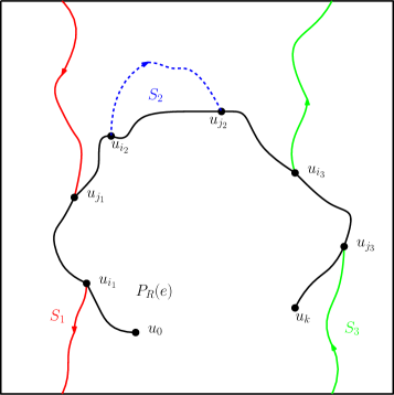
Figure 24: Situation of Lemma 51.

Lemma 52.

$$\left|Q\right|\geq\left|P_{R}(e)\right|-2n_{LR_{\ell}}(Q,e)-3n_{RL_{\ell}}(Q,e)-922.$$

Proof.

By Lemmas 47, we have

$$|Q|=\sum_{q=1}^{t}\left|S_{q}\right|\geq\left|P_{R}(e)\right|-2n_{LR_{\ell}}(Q,e)-3n_{RL_{\ell}}(Q,e)-5n_{LL_{\ell}}(Q,e)-2n_{LL_{n}}^{Y}(Q,e)-{13\times|Z|}.$$

Thus we obtain the lemma by Lemmas 49 and 51 and since $|X|\leq 72$. ∎

Lemma 53.

Consider $q_{1},q_{2}\in Y$, such that $q_{1}\neq q_{2}$ and $S_{q_{1}},S_{q_{2}}$ are both of type $LR_{l}$ or $RL_{\ell}$. If $S_{q_{1}}$, $S_{q_{2}}$ have extremities $(u_{i_{1}},u_{j_{1}})$ and $(u_{i_{2}},u_{j_{2}})$ with $i_{1}<j_{1}$, $i_{2}<j_{2}$ and $i_{1}<i_{2}$, then $q_{1}<q_{2}$.

Proof.

Suppose by contradiction that $q_{1}>q_{2}$. Let $p_{1}$, $p_{2}$ be the length of $S_{q_{1}}$ and $S_{q_{2}}$. By Lemma 47, we have $p_{1}\geq j_{1}-i_{1}-3$ and $p_{2}\geq j_{2}-i_{2}-3$. Since $q_{2}<q_{1}$, we have $i_{2}\neq j_{1}$. We consider the two following cases: $i_{2}<j_{1}$ or $j_{1}<i_{2}$.

• If $i_{2}<j_{1}$: We have $|Q[i_{2},j_{1}]|\geq p_{1}+p_{2}+1\geq p_{2}+2$. Since $Q$ is a shortest path, we have $|P_{R}(e)[j_{1},j_{2}]|\geq|Q[j_{2},j_{1}]|\geq p_{1}+1\geq 2$. We obtain the following contradiction:

  $$|P_{R}(e)[i_{2},j_{1}]|=|P_{R}(e)[i_{2},j_{2}]|-|P_{R}(e)[j_{1},j_{2}]|\leq j_{2}-i_{2}-2\leq p_{2}+1\leq|Q[i_{2},j_{1}]|-1.$$

• If $j_{1}<i_{2}$: Let $q_{0}=\max\{q\in[\![q_{1},q_{2}[\![\ :\text{the extremities }i,j\textrm{ of }S_{q}\textrm{ are such that }i\leq j_{1}\leq j\}$. Let $(u_{i_{0}},u_{j_{0}})$ be the extremities of $S_{q_{0}}$ with $i_{0}\leq j_{1}\leq j_{0}$. Let $p_{0}$ be the length of $S_{q_{0}}$. Since $i_{0}\leq j_{1}\leq j_{0}$, by definition of $Y$ and Lemma 48, we have that $S_{q_{0}}$ is not of type $h$. By Lemma 47, we have $p_{0}\geq j_{0}-i_{0}-5$. Moreover, we have $|Q[i_{0},j_{1}]|\geq p_{0}+p_{1}+p_{2}+1\geq p_{0}+3$. Since $Q$ is a shortest path, we have $|P_{R}(e)[j_{0},j_{1}]|\geq p_{1}+p_{2}+1\geq 3$. We obtain the following contradiction:

  $$|P_{R}(e)[i_{0},j_{1}]|=|P_{R}(e)[i_{0},j_{0}]|-|P_{R}(e)[j_{0},j_{1}]|\leq j_{0}-i_{0}-3\leq p_{0}+2\leq|Q[i_{0},j_{1}]|-1.$$

∎

We now state a lemma which is analogous to Proposition $11$ and Proposition $12$ of [1].

Consider $C$ a contractible cycle of $G$, given with a traversal direction. Then $C$ separates the map $G$ into two regions. We define $V_{\ell}(C)$ (respectively $V_{r}(C)$) the set of vertices lying in the region on the left (resp. right) side of $C$, including $C$. The graphs $G[V_{\ell}(C)]$ and $G[V_{r}(C)]$ denotes the subgraph of $G$ induced by these set of vertices.

Lemma 54.

If $n_{LR_{\ell}}(Q,e)>3$ (resp. $n_{RL_{\ell}}(Q,e)>3$), then there exists a contractible cycle $C$ in $G$, given with a direction of traversal, of length at most $\frac{6|Q|}{n_{LR_{\ell}}(Q,e)-3}+2$ (resp. $\frac{6|Q|}{n_{RL_{\ell}}(Q,e)-3}+3$) such that for all $\iota\in\{\ell,r\}$, we have $\max_{u\in V_{\iota}(C)}m(u)-\min_{u\in V_{\iota}(C)}m(u)$ is at least $\lfloor n_{LR_{\ell}}(Q,e)/3\rfloor-{79}$ (resp. $\lfloor n_{RL_{\ell}}(Q,e)/3\rfloor-{79}$).

Proof.

We prove the lemma for $n_{LR_{\ell}}(Q,e)>3$ (the proof for $n_{RL_{\ell}}(Q,e)>3$ is similar). For $1\leq q\leq t$, let $n_{LR_{\ell}}(q)$ be the number of sub-paths of type $LR_{\ell}$ among $\{S_{1},\cdots,S_{q}\}$. Let $s=\left\lfloor n_{LR_{\ell}}(Q,e)/3\right\rfloor$. Let $Z$ be the set of elements $1\leq q\leq t$, such that $S_{q}$ is of type $LR_{\ell}$ and $s+1\leq n_{LR_{\ell}}(q)\leq 2s$. Let $q^{\star}\in Z$ such that $|S_{q^{\star}}|=\min\{|S_{q}|\,:\,q\in Z\}$. Let $S_{q^{\star}}=(w_{0},...,w_{p})$ with $w_{0}=u_{i}$, $w_{p}=u_{j}$ for some $0\leq i<j\leq k$ and let $C=(w_{0},\ldots,w_{p}=u_{j},\ldots,u_{i})$. Then

$$|Q|\geq s\,p\geq\frac{n_{LR_{\ell}}(Q,e)-3}{3}p$$

By Lemma 47, we have $p\geq j-i-2$. Then $|C|=p+j-i\leq 2p+2\leq\frac{6|Q|}{n_{LR_{\ell}}(Q,e)-3}+2$ edges.

Finally, by Lemma 53, one of $G[V_{\ell}(C)]$ or $G[V_{r}(C)]$ contains all sub-paths of type $LR_{\ell}$ among $(S_{1},\cdots,S_{q^{\star}}){\bigcap\left\{\bigcup_{i\in Y}S_{i}\right\}}$ and the other contains all sub-paths of type $LR_{\ell}$ among $(S_{q\star},\cdots,S_{t}){\bigcap\left\{\bigcup_{i\in Y}S_{i}\right\}}$. Therefore, each of $G[V_{\ell}(C)]$ and $G[V_{r}(C)]$ contains at least $s-18\times 4$ vertices of $P_{R}(e)$. By Lemmas 43 and 5, we obtain $\max_{u\in V_{\iota}(C)}m(u)-\min_{u\in V_{\iota}(C)}m(u)\geq s-72-7$ for all $\iota\in\{\ell,r\}$. ∎

A.2 Approximation of distances by labels

As in Section 10, for $n\geq 1$, let $G_{n}$ be a uniformly random element of $\mathcal{G}(n)$. Let $d_{n}$ denote the graph distance $d_{G_{n}}$. Recall that $\Phi$ denotes the bijection from $\mathcal{T}_{r,s,b}(n)$ to $\mathcal{G}(n)$ of Theorem 3. Let $T_{n}=\Phi^{-1}(G_{n})$. Therefore $T_{n}$ is a uniformly random element of $\mathcal{T}_{r,s,b}(n)$.

We need several definitions similar to Section 3. Let $V_{n}$ be the set of vertices of $T_{n}$. Let $a_{n}^{0}$ be the root angle of $T_{n}$ and $v^{0}_{n}$ be its root vertex. Let $\ell_{n}=4n+1$. We define $\Gamma_{n}$ as the unicellular map obtained from $T_{n}$ by adding a special dangling half-edge, called the root half-edge, incident to the root angle of $T_{n}$. The root angle of $\Gamma_{n}$, still noted $a_{n}^{0}$, is the angle of $\Gamma_{n}$ just after the root half-edge in counterclockwise order around its incident vertex. Let $A_{n}=(a_{n}^{0},\ldots,a_{n}^{\ell})$ be the sequence of consecutive angles of $\Gamma_{n}$ in clockwise order around the unique face of $\Gamma_{n}$ starting from $a_{n}^{0}$. Let $\lambda_{n}$ be the labeling function of $\Gamma_{n}$ as defined in Section 3. For each vertex $u$ of $V_{n}$, let $m_{n}(u)$ be the minimum of the labels incident to $u$.

The main result of this section is the following:

Theorem 5.

For all $\epsilon>0$, we have

$$\lim_{n\rightarrow\infty}\mathbb{P}\left(\exists u\in V_{n}:|d_{n}(u,v_{n}^{0})-m_{n}(u)|>\epsilon\,n^{1/4}\right)=0.$$

Before going into the proof, we need some additional notations. For $0\leq i\leq\ell_{n}$, let $r_{n}(i)$ be the vertex of $V_{n}$ incident to angle $a_{n}^{i}$ (i.e the vertex contour function of $\Gamma$). Given an integer $0\leq i\leq\ell_{n}$ and $\Delta>0$, we denote

$$p_{n}(i,\Delta) =\max(\{0\}\cup\left\{j<i:\left|m_{n}(r_{n}(j))-m_{n}(r_{n}(i))\right|\geq\Delta\right\}),$$

$$q_{n}(i,\Delta) =\min(\{\ell_{n}\}\cup\left\{j>i:\left|m_{n}(r_{n}(j))-m_{n}(r_{n}(i))\right|\geq\Delta\right\})\;\text{and}$$

$$N_{n}(i,\Delta) =|\left\{r_{n}(j):\exists j\in\llbracket p_{n}(i,\Delta),q_{n}(i,\Delta)\rrbracket\right\}|.$$

The proof of the following lemma is omitted, it is almost identical to [1, Lemma $8.2$]:

Lemma 55.

For all $\epsilon>0$ and $\beta>0$, there exists $\alpha>0$ and $n_{0}\in\mathbb{N}$ such that for every $n\geq n_{0}$,

$$\mathbb{P}\left(\inf\left\{N_{n}(i,\beta n^{1/4}):0\leq i\leq 2n+1\right\}\geq\alpha n\right)\geq 1-\epsilon.$$

We are now ready to prove the main theorem of this section.

Proof of Theorem 5.

By Lemma 7, for $n\geq 1$ and $u\in V_{n}$, we have $d_{n}(v_{n}^{0},u)\leq m_{n}(u)$. So it suffices to prove that for all $\epsilon>0$

$$\lim_{n\rightarrow\infty}\mathbb{P}\left(\exists u\in V_{n}:d_{n}(v_{n}^{0},u)<m_{n}(u)-\epsilon\,n^{1/4}\right)=0.$$

This is equivalent to show that for all $\epsilon>0$,

$$\limsup_{n\rightarrow\infty}\mathbb{P}\left(\exists u\in V_{n}:d_{n}(v^{0}_{n},u)<m(u)-15\epsilon n^{1/4}+964\right)\leq 4\epsilon.$$

Denote by $\mathop{\mathrm{diam}}(G_{n})$ the diameter of the graph $G_{n}$. Consider $\epsilon>0$. By Lemma 41, there exists $y>0$ such that $\mathbb{P}\{\mathop{\mathrm{diam}}(G_{n})\geq yn^{1/4}\}<\epsilon$.

Now, assume that there exists $n_{0}\in\mathbb{N}$, such that for all $n\geq n_{0}$, there exists $u_{n}\in V_{n}$ such that $d_{G_{n}}(u_{n},v_{n}^{0})<m(u_{n})-15\epsilon n^{1/4}-964$. Consider the canonical orientation of $G_{n}$ and let $e_{n}$ be an outgoing edge of $u_{n}$. With the notations of Section A.1, let $P_{n}=P_{R}(e_{n})$ be the right-to-root path starting at $e_{n}$. Let $Q_{n}$ be a shortest path from $u_{n}$ to $v_{n}^{0}$ that maximizes the number of common edges with $P_{n}$.

By Lemmas 46 and 52, we have

$$2n_{LR_{\ell}}(Q_{n},e_{n})+3n_{RL_{\ell}}(Q_{n},e_{n})\geq \left|P_{n}\right|-\left|Q_{n}\right|-922$$

$$\geq (m_{n}(u)-42)-(m_{n}(u)-15\epsilon n^{1/4}-964)-922$$

$$\geq 15\epsilon n^{1/4}$$

Thus for $n_{0}$ large enough we have (for each $n\geq n_{0}$) either $n_{LR_{\ell}}(Q_{n},e_{n})\geq\max(3,3\epsilon n^{1/4})$ or $n_{RL_{\ell}}(Q_{n},e_{n})\geq\max(3,3\epsilon n^{1/4})$. We call $B_{n}$ the event $G_{n}$ contains a contractile cycle $C$ of length at most $(2y/\epsilon+4)$, given with a traversal direction, such that for both $\iota\in\{l,r\}$, we have

$$\max_{u\in V_{\iota}(C)}m_{n}(u)-\min_{u\in V_{\iota}(C)}m_{n}(u)\geq\epsilon n^{1/4}-79.$$

We deduce from Lemma 54 that, for $n_{0}$ large enough and all $n\geq n_{0}$, either $\mathop{\mathrm{diam}}(G_{n})\geq yn^{1/4}$ or $B_{n}$ occurs.

Therefore it suffices to prove that

$$\mathbb{P}(B,\mathop{\mathrm{diam}}(G_{n})\leq yn^{1/4})\leq 3\epsilon.$$

Consider $n\geq n_{0}$ such that $B$ occurs. Let $C$ be as in the definition of $B$. Let $F$ be the subgraph of $T_{n}$ induced by $V(G_{n})\setminus V(C)$. Recall that $G_{n}[V_{l}(C)]$ (resp. $G_{n}[V_{r}(C)]$) is the sub-graph of $G_{n}$ induced by $V_{l}(C)$ (resp. $V_{r}(C)$). Then each component of $F$ is contained in $G_{n}[V_{l}(C)]$ or $G_{n}[V_{r}(C)]$. By Lemma 6, for $\{u,v\}\in E(G_{n})$ we have $|m(u)-m(v)|\leq 7$. It follows that, for $\iota\in\{l,r\}$, there exists one component $F_{\iota}$ of $F$ such that

$$\max_{u\in V(F_{\iota})}m_{n}(u)-\min_{u\in V(F_{\iota})}m_{n}(u)\geq\epsilon^{2}n^{1/4}/(2y+4\epsilon)-79.$$

Using again Lemma 6, then for $\iota\in\{l,r\}$, there exists $v_{\iota}\in F_{\iota}$ such that

$$\min_{v\in V(C)}|m(v_{\iota})-m(v)|\geq \left(\frac{\epsilon^{2}n^{1/4}}{2y+4\epsilon}-79\right)\big{/}2-7-(2y/\epsilon+2)\times 7$$

$$\geq\frac{\epsilon^{2}n^{1/4}}{4y+8\epsilon}-19-14y/\epsilon.$$

Now for $\iota\in\{\ell,r\}$, let $j_{\iota}=\inf\{0\leq i\leq\ell_{n}:r_{n}(i)=v_{\iota}\}$. Fix any $\beta\in(0,\epsilon^{2}/(4y+8\epsilon))$. By Lemma 55, there exists $\alpha>0$ such that for $n$ large enough,

$$\mathbb{P}\left(\min\{|N_{n}(j_{\ell},\beta n^{1/4})|,|N_{n}(j_{r},\beta n^{1/4})|\}\leq\alpha n\right)\leq\epsilon.$$

For $n$ sufficiently large, we have $\frac{\epsilon^{2}n^{1/4}}{4y+8\epsilon}-19-14y/\epsilon>\beta n^{1/4}$. Then we have for $\iota\in\{\ell,r\}$, $N(j_{\iota},\beta n^{1/4})\subset V_{\iota}(C)$. It follows that for $n$ large enough,

$$\mathbb{P}(B,\mathop{\mathrm{diam}}(G_{n})\leq yn^{1/4})\leq$$

$$\epsilon+\mathbb{P}\left(\exists C\text{ contractile cycle},|C|\leq 2y/\epsilon+4,\min\{|V_{l}(C)|,|V_{r}(C)|\}\geq\alpha n\right).$$

The event $\{\exists C\text{ contractile cycle},|C|\leq 2y/\epsilon+4,\min\{|V_{l}(C)|,|V_{r}(C)|\}\geq\alpha n\}$ means that $G_{n}$ contains a separating contractile cycle of length at most $2y/\epsilon+4$ that separates $G_{n}$ into two sub-triangulations both of size at least $\alpha n$. It remains to prove that this has probability going to $0$ when $n$ goes to infinity. Let $p_{n,m}$ (resp. $t_{n,m}$) be the number of simple triangulation of an $m$-gon with $n$ inner vertices (resp. the number of essentially simple toroidal maps on the torus with $n$ vertices, such that all faces have size three except one that has size $m$), rooted at a maximal triangle. From previously known estimates, there exist two constants $A_{m}$ (see [7]) and $B_{m}$ (by Corollary 1) such that

$$p_{n,m}\leq A_{m}n^{-5/2}\left(\frac{256}{27}\right)^{n}\quad\text{and}\quad{t}_{n,m}\leq B_{m}\left(\frac{256}{27}\right)^{n}$$

(the upper bound for $p_{n,m}$ estimates the number of arbitrarily rooted triangulations, of which there are more than the type counted by $p_{n,m}$ itself).

Let $\Gamma_{n}$ be the event $G_{n}$ contains a separating contractile cycle of length at most $2y/\epsilon+4$ that separates $G_{n}$ into two sub-triangulations both of size at least $\alpha n$. We have:

$$\mathbb{P}(\Gamma_{n}) \leq\Upsilon^{-1}\left(\frac{256}{27}\right)^{-n}\sum_{k=3}^{\lfloor 2y/\epsilon+4\rfloor}\sum_{\ell=\lfloor\alpha n\rfloor}^{\lfloor(1-\alpha)n\rfloor}p_{\ell,k}{t}_{n-\ell,k}$$

$$\leq\Upsilon^{-1}\left(\frac{256}{27}\right)^{-n}\sum_{k=3}^{\lfloor 2y/\epsilon+4\rfloor}\sum_{\ell=\lfloor\alpha n\rfloor}^{\lfloor(1-\alpha)n\rfloor}A_{k}\ell^{-5/2}\left(\frac{256}{27}\right)^{\ell}B_{k}\left(\frac{256}{27}\right)^{n-\ell}$$

$$\leq\Upsilon^{-1}\sum_{k=3}^{\lfloor 2y/\epsilon+4\rfloor}A_{k}B_{k}\sum_{\ell=\lfloor\alpha n\rfloor}^{\lfloor(1-\alpha)n\rfloor}\ell^{-5/2}\leq\Upsilon^{-1}\sum_{k=3}^{\lfloor 2y/\epsilon+4\rfloor}A_{k}B_{k}\;n\;(\alpha n)^{-5/2}.$$

Therefore $\mathbb{P}(\Gamma_{n})$ converges towards $0$ when $n$ goes to infinity, which concludes the proof of the Theorem. ∎

References

- [1] L. Addario-Berry and M. Albenque, The scaling limit of random simple triangulations and random simple quadrangulations, Annals of Probability, 45 (2017), pp. 2767–2825.
- [2] D. Aldous, The continuum random tree ii: an overview, Stochastic analysis, 167 (1991), pp. 23–70.
- [3] J. Bertoin, L. Chaumont, and J. Pitman, Path transformations of first passage bridges, Electronic Communications in Probability, 8 (2003), pp. 155–166.
- [4] J. Bettinelli, Scaling limits for random quadrangulations of positive genus, Electronic Journal of Probability, 15 (2010), pp. 1594–1644.
- [5] J. Bettinelli and G. Miermont, Personal communication. 2019.
- [6] P. Billingsley, Convergence of probability measures, John Wiley & Sons, 2013.
- [7] W. G. Brown, Enumeration of triangulations of the disk, Proceedings of the London Mathematical Society, 3 (1964), pp. 746–768.
- [8] D. Burago, Y. Burago, I. D. Burago, and S. Ivanov, A course in metric geometry, vol. 33, American Mathematical Soc., 2001.
- [9] G. Chapuy, M. Marcus, and G. Schaeffer, A bijection for rooted maps on orientable surfaces, SIAM Journal on Discrete Mathematics, 23 (2009), pp. 1587–1611.
- [10] P. Chassaing and G. Schaeffer, Random planar lattices and integrated superbrownian excursion, Probability Theory and Related Fields, 128 (2004), pp. 161–212.
- [11] N. Dershowitz and S. Zaks, The cycle lemma and some applications, European Journal of Combinatorics, 11 (1990), pp. 35–40.
- [12] V. Despré, D. Gonçalves, and B. Lévêque, Encoding toroidal triangulations, Discrete & Computational Geometry, 57 (2017), pp. 507–544.
- [13] P. Fitzsimmons, J. Pitman, and M. Yor, Markovian bridges: construction, palm interpretation, and splicing, in Seminar on Stochastic Processes, 1992, Springer, 1993, pp. 101–134.
- [14] D. Gonçalves, K. B. Knauer, and B. Lévêque, Structure of schnyder labelings on orientable surfaces, CoRR, abs/1501.05475 (2015).
- [15] D. Gonçalves and B. Lévêque, Toroidal maps: Schnyder woods, orthogonal surfaces and straight-line representations, Discrete & Computational Geometry, 51 (2014), pp. 67–131.
- [16] J.-F. Le Gall, The topological structure of scaling limits of large planar maps, Inventiones mathematicae, 169 (2007), pp. 621–670.
- [17] J.-F. Le Gall et al., Uniqueness and universality of the brownian map, The Annals of Probability, 41 (2013), pp. 2880–2960.
- [18] B. Lévêque, Generalization of schnyder woods to orientable surfaces and applications, Habilitation manuscript, arXiv:1702.07589, (2017).
- [19] G. Miermont, The brownian map is the scaling limit of uniform random plane quadrangulations, Acta mathematica, 210 (2013), pp. 319–401.
- [20] J. Neveu, Arbres et processus de galton-watson, Ann. Inst. H. Poincaré Probab. Statist, 22 (1986), pp. 199–207.
- [21] V. V. Petrov, Limit theorems of probability theory: sequences of independent random variables, (1995).
- [22] V. V. Petrov, Sums of independent random variables, vol. 82, Springer Science & Business Media, 2012.
- [23] D. Poulalhon and G. Schaeffer, Optimal coding and sampling of triangulations, Algorithmica, 46 (2006), pp. 505–527.
- [24] D. Revuz and M. Yor, Continuous martingales and Brownian motion, vol. 293, Springer Science & Business Media, 2013.
- [25] O. Schramm, Conformally invariant scaling limits, in Proceedings of the International Congress of Mathematicians, Madrid, 2006.