Controlled exploration of chemical space by machine learning of coarse-grained representations

Abstract

The size of chemical compound space is too large to be probed exhaustively. This leads high-throughput protocols to drastically subsample and results in sparse and non-uniform datasets. Rather than arbitrarily selecting compounds, we systematically explore chemical space according to the target property of interest. We first perform importance sampling by introducing a Markov chain Monte Carlo scheme across compounds. We then train a machine learning (ML) model on the sampled data to expand the region of chemical space probed. Our boosting procedure enhances the number of compounds by a factor 2 to 10, enabled by the ML model’s coarse-grained representation, which both simplifies the structure-property relationship and reduces the size of chemical space. The ML model correctly recovers linear relationships between transfer free energies. These linear relationships correspond to features that are global to the dataset, marking the region of chemical space up to which predictions are reliable—a more robust alternative to the predictive variance. Bridging coarse-grained simulations with ML gives rise to an unprecedented database of drug-membrane insertion free energies for 1.3 million compounds.

I Introduction

Computational high-throughput screening ever-increasingly allows the coverage of larger subsets of chemical space. Extracting a property of interest across many compounds helps infer structure-property relationships, of interest both for a better understanding of the physics and chemistry at hand, as well as for materials design Pyzer-Knapp et al. (2015); Jain et al. (2016); Bereau et al. (2016); von Lilienfeld (2018). Recent hardware and algorithmic developments have enabled a number of applications of high-throughput screening in hard condensed matter Curtarolo et al. (2013); Ghiringhelli et al. (2015), while comparatively slower development in soft matter Ferguson (2017); Bereau (2018).

Soft-matter systems hinge on a delicate balance between enthalpic and entropic contributions, requiring proper computational methods to reproduce them faithfully. Physics-based methodologies, in particular molecular dynamics (MD), provide the means to systematically sample the conformational ensemble of complex systems. High-throughput screening using MD presumably involves one simulation per compound. This remains computationally prohibitive at an atomistic resolution.

As an alternative, we recently proposed the use of coarse-grained (CG) models to establish a high-throughput scheme. Coarse-grained models lump several atoms into one bead to decrease the number of degrees of freedom Noid (2013). The computational benefit of a high-throughput coarse-grained (HTCG) framework is two-fold: ($i$) faster sampling of conformational space; but most importantly ($ii$) a significant reduction in the size of chemical space, tied to the transferable nature of the CG model (i.e., a finite set of bead types). Effectively the reduction in chemical space due to coarse-graining still leads to a combinatorial explosion of chemical space, but with a significantly smaller prefactor. This many-to-one mapping is empirically probed by coarse-graining large databases of small molecules—an effort made possible by automated force-field parametrization schemes Bereau and Kremer (2015). Using the CG Martini force field Periole and Marrink (2013), we recently reported the exhaustive characterization of CG compounds made of one and two beads, corresponding to small organic molecules between 30 and 160 Da. Running HTCG for 119 CG compounds enabled the predictions of drug-membrane thermodynamics Menichetti et al. (2017) and permeability Menichetti et al. (2019) for more than $500,000$ small organic molecules.

Pushing further our exploration of chemical space, how do we further diversify the probed chemistry in a systematic manner? Scaling up to larger molecular weight using more CG beads will ultimately lead to a combinatorial explosion: there are already 1,470 linear trimers and 19,306 linear tetramers in Martini. Instead of an exhaustive enumeration, we propose to explore regions of chemical space that are of particular interest. Specifically, rather than following the chemistry we navigate chemical space according to a target property—in this work, the tendency of a small organic molecule to partition at the interface of a phospholipid bilayer.

Akin to importance sampling used extensively to characterize conformational space, we first introduce a Markov chain Monte Carlo (MC) procedure to sample chemical compound space. Our methodology consists of a sequence of compounds where trial alchemical transformations are accepted according to a Metropolis criterion (Fig. 1a). While the acceptance criterion for conformational sampling typically includes the energy of the system, compositional sampling (i.e., across chemical space) means averaging over the environment and thus calls for a free energy. As such, MC moves will push the exploration towards small molecules that increase their stability within a specific condensed-phase environment—algorithmically akin to constant pH simulations Mongan et al. (2004).

In this work we focus on the free-energy difference of transferring a small molecule from the aqueous environment to the lipid-membrane interface (Fig. 1b). The MC acceptance criterion is here dictated by pharmacokinetic considerations: while hydrophobic compounds will more easily permeate through the bilayer Menichetti et al. (2019), they may display poor solubility properties Dahan et al. (2016). Our MC criterion thus aims at balancing the delicate interplay between solubility and permeability.

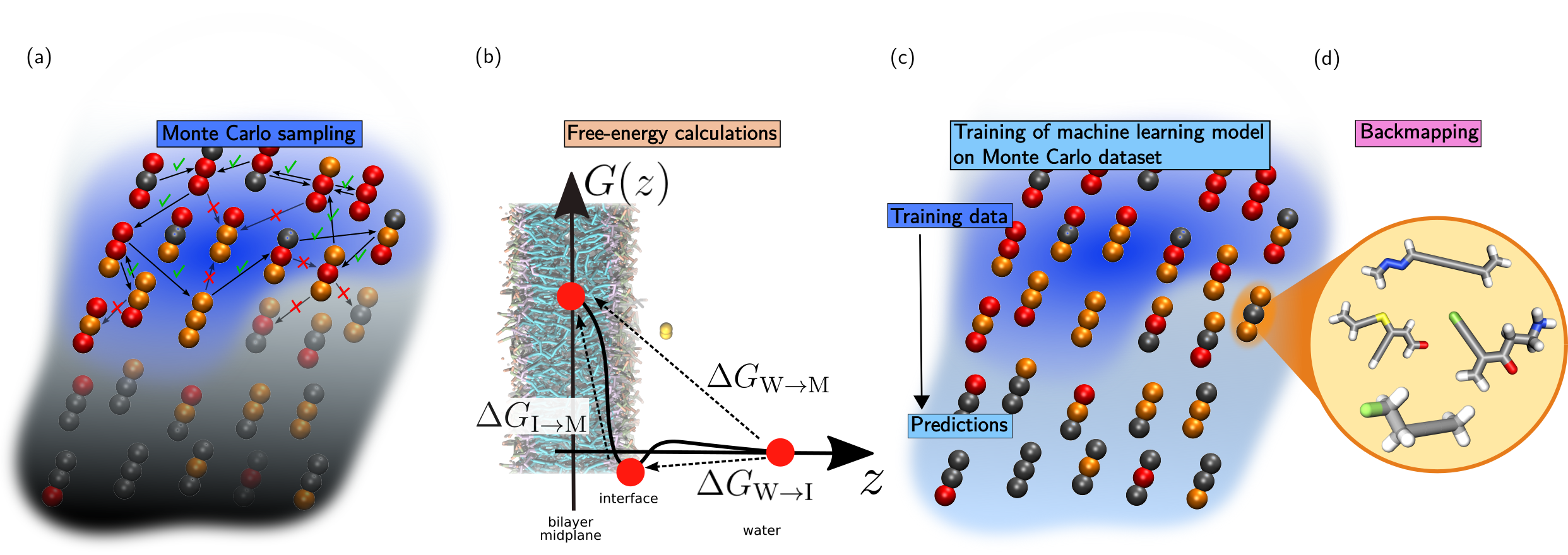
Figure 1: (a) Importance sampling across coarse-grained compounds via a Markov chain Monte Carlo scheme. Only the dark-blue region is sampled. (b) Background: Simulation setup of a solute (yellow) partitioning between water (not shown) and the lipid membrane. Foreground: Potential of mean force along the normal of the bilayer, $G(z)$, and definition of the three transfer free energies of interest between the three state points (red circles): bilayer midplane (“M”), membrane-water interface (“I”), and bulk water (“W”). (c) The MC-sampled free energies (dark-blue region) form the training set for a machine learning model, used to predict a larger subset of compounds (light-blue region). (d) Each coarse-grained compound represents a large number of small molecules.

To further boost the size of chemical space that is probed, we further predict a more extended subset of compounds that were not sampled by using machine learning (ML; see Fig. 1c) Rasmussen (2004). Despite known limited capabilities to extrapolate beyond the training set, we observe remarkable accuracy for the predicted compounds. This excellent transferability can be associated to a simplified learning procedure at the CG resolution: structure-property relationships are easier to establish Menichetti et al. (2019) and compound similarity is compressed due to the reduction of chemical space. The range of reliable predictions is made clear by means of the ML model satisfying linear thermodynamic relations across compounds Menichetti et al. (2017)—a more robust confidence metric compared to the predictive variance. The CG results are then systematically backmapped (Fig. 1d) to yield an unprecedentedly-large database of free energies.

II Methods

II.1 Coarse-grained simulations

MD simulations of the Martini force field Periole and Marrink (2013) were performed in Gromacs 5.1. The integration time-step was $\delta t=0.02~{}\tau$, where $\tau$ is the model’s natural unit of time. Control over the system temperature and pressure ($T=300~{}K$ and $P=1$ bar) was obtained by means of a velocity rescaling thermostat Bussi et al. (2007) and a Parrinello-Rahman barostat Parrinello and Rahman (1981), with coupling constants $\tau_{T}=~{}\tau$ and $\tau_{P}=12~{}\tau$. Bulk simulations consisted of $N_{\textup{W}}=450$ and $N_{\textup{O}}=336$ water and octane molecules, where the latter was employed as a proxy for the hydrophobic core of the bilayer Menichetti et al. (2017). As for interfacial simulations, a membrane of $36~{}\text{nm}^{2}$ containing $N_{\textup{L}}=128$ 1,2-dioleoyl-sn-glycero-3-phosphocholine (DOPC) lipids (64 per layer) and $N_{\textup{W}}^{\prime}=1890$ water molecules was generated by means of the Insane building tool Wassenaar et al. (2015), and subsequently minimized, heated up, and equilibrated. In all simulations containing water molecules we added an additional $10\%$ of antifreeze particles.

II.2 Free-energy calculations

Water/interface and interface/membrane transfer free energies $\Delta G_{\textup{W}\rightarrow\textup{I}}$ and $\Delta G_{\textup{I}\rightarrow\textup{M}}$ for all compounds investigated in this work were obtained from alchemical transformations, in analogy with Ref. Menichetti et al. (2017). This construction is based on the relation linking the transfer free energies of two compounds $A$ and $B$ ($\Delta G^{A}_{\textup{W}\rightarrow\textup{I}}$, $\Delta G^{B}_{\textup{W}\rightarrow\textup{I}}$ and $\Delta G^{A}_{\textup{I}\rightarrow\textup{M}}$, $\Delta G^{B}_{\textup{I}\rightarrow\textup{M}}$) to the free energies of alchemically transforming $A$ into $B$ in the three fixed environments, $\Delta G^{A\rightarrow B}_{\textup{I}}$, $\Delta G^{A\rightarrow B}_{\textup{W}}$ and $\Delta G^{A\rightarrow B}_{\textup{M}}$

$$\Delta G^{B}_{\textup{W}\rightarrow\textup{I}}=\Delta G^{A}_{\textup{W}\rightarrow\textup{I}}+(\Delta G^{A\rightarrow B}_{\textup{I}}-\Delta G^{A\rightarrow B}_{\textup{W}}),$$

$$\Delta G^{B}_{\textup{I}\rightarrow\textup{M}}=\Delta G^{A}_{\textup{I}\rightarrow\textup{M}}+(\Delta G^{A\rightarrow B}_{\textup{M}}-\Delta G^{A\rightarrow B}_{\textup{I}}).$$ (1)

$\Delta G^{A\rightarrow B}_{\textup{I}}$, $\Delta G^{A\rightarrow B}_{\textup{W}}$, and $\Delta G^{A\rightarrow B}_{\textup{M}}$ were determined by means of separate MD simulations at the interface, in bulk water, and in bulk octane. For the calculation of each $\Delta G^{A\rightarrow B}_{i}$, $i={\textup{I}},{\textup{W}},{\textup{M}}$ we relied on the multistate Bennett acceptance ratio (MBAR) Shirts and Chodera (2008); Klimovich et al. (2015), in which free-energy differences are obtained by combining together the results from simulations that sample the statistical ensemble of a set of interpolating Hamiltonians $H(\lambda)$, $\lambda\in[0,1]$, with $H(0)=H_{A}$ and $H(1)=H_{B}$. We employed 24 evenly spaced $\lambda$-values for each alchemical transformation and in each environment (interface, water, octane). The production time for each $\lambda$ point was $4\cdot 10^{4}~{}\tau$ at the interface and $2\cdot 10^{4}~{}\tau$ in bulk environments. To calculate $\Delta G^{A\rightarrow B}_{\textup{I}}$ we added a harmonic potential with $k=240~{}{\rm kcal}\,{\rm mol}^{-1}\,{\rm nm}^{-2}$ between the compound’s center of mass and the bilayer midplane at a distance $\bar{z}=1.5~{}{\rm nm}$, to account for the spatial localization of the interface. The value of $\bar{z}$ was fixed by analyzing the potential of mean force $G(z)$ (see Fig. 1b) for the insertion of various solutes that preferentially sit near the lipid headgroups in a DOPC bilayer Menichetti et al. (2017). The minimum of these profiles was found to be located at $\bar{z}\approx 1.8~{}{\rm nm}$ irrespective of the compound’s chemical detail, suggesting that the location of the dip is largely determined by the membrane environment. In this work, we corrected $\bar{z}$ to account for the horizontal shift in the potentials of mean force generated by the additional bead of the Martini DOPC model originally employed in Ref. Menichetti et al., 2017 Menichetti et al. (2018).

We further emphasize that we only restrained the compound’s center of mass, while the orientation of the linear molecule with respect to the bilayer normal was left unbiased. Notably, we do expect (and observed) compounds to display very different preferential orientations—from parallel to perpendicular with respect to the bilayer normal. There are two reasons motivating our choice: ($i$) the CG simulations efficiently explore conformational space anyway, such that this degree of freedom is relatively easily sampled; and ($ii$) the information between interpolating Hamiltonians that are simulated during an alchemical transformation are efficiently exchanged thanks to the MBAR method. The small corrections operated during the thermodynamic-cycle optimization we apply a posteriori attest of our assumptions.

II.3 Monte Carlo sampling

We perform a stochastic exploration of the chemical space of CG linear trimers and tetramers through the generation of Markovian sequences of compounds. Given the last compound $A$ of a sequence, the new compound $B$ is proposed by randomly selecting a bead of $A$ and changing its type. The move from $A$ to $B$ is then accepted with probability

$$P_{A\rightarrow B}=\min\left\{1,\exp\left[-\beta(\Delta G^{B}_{\textup{W}\rightarrow\textup{I}}-\Delta G^{A}_{\textup{W}\rightarrow\textup{I}})\right]\right\},$$ (2)

where $\Delta G^{A}_{\textup{W}\rightarrow\textup{I}}$ and $\Delta G^{B}_{\textup{W}\rightarrow\textup{I}}$ are the water/interface transfer free energies of $A$ and $B$, respectively. $P_{A\rightarrow B}$ aims at driving the Monte Carlo sampling towards compounds that favor partitioning at the membrane interface (Fig. 1b). This is significantly different from optimizing $\Delta G_{\textup{W}\rightarrow\textup{M}}$, because those would likely be poorly soluble in an aqueous environment Dahan et al. (2016).

While in this work we set $\beta=1/k_{\mathrm{B}}T$, we stress that $\beta$ can in principle be chosen independently of the system temperature. The free-energy difference in Eq. 2 is derived from the alchemical free-energy differences of transforming $A$ into $B$ in the three fixed environments $\Delta G^{A\rightarrow B}_{i},~{}i=\textup{W, I, M}$ (first relation in Eq. 1), which we compute from MD simulations.

We generated up to five independent Markovian sequences in parallel, each starting from a different initial compound. To avoid recalculating alchemical transformations already visited, we stored the history of calculations and looked up previously-calculated values when available.

II.4 Thermodynamic-cycle optimization

By combining together the results of all independent Markovian sequences, the outcome of our Monte Carlo sampling consists of an alchemical network. Each node of the network represents a compound, and an edge connecting two nodes $A$ and $B$ corresponds to an alchemical transformation that was sampled via an MD simulation, see Fig. 2. Each edge is characterized by the free-energy differences $\Delta G^{A\rightarrow B}_{\textup{i}}$ in the three fixed environments, $i=\textup{W, I, M}$. The network representation was created with NetworkX Hagberg et al. (2008) and visualized with Gephi Bastian et al. (2009).

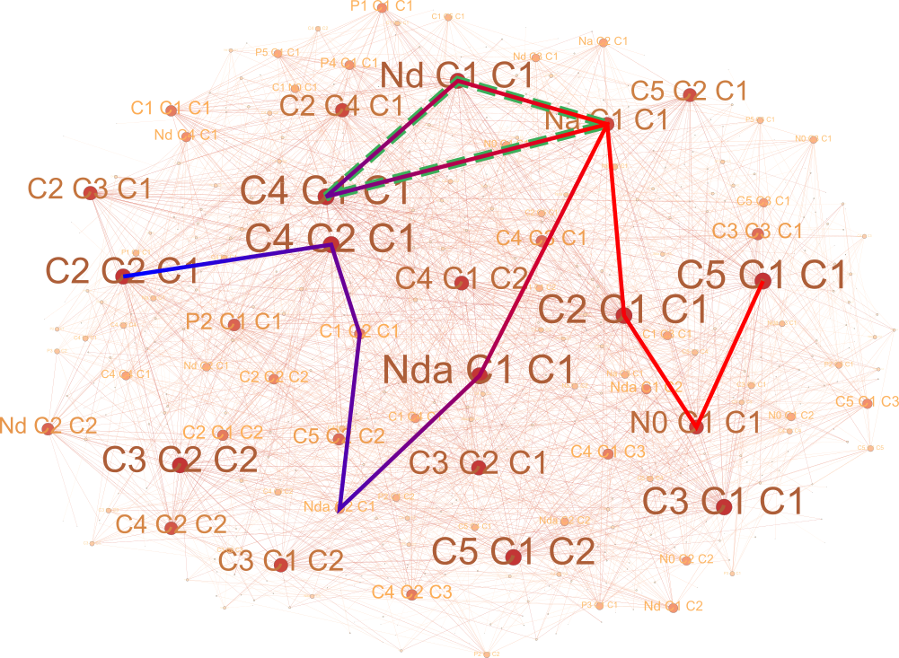
Figure 2: Network of CG compounds, each denoted by its set of Martini bead types. Their size is proportional to the number of edges. The blue-to-red path illustrates a sequence of accepted compounds sampled from the Monte Carlo scheme. The dashed, green triangle denotes a closed path in compound space. Sampling all of its three branches closes the thermodynamic cycle, used as constraint to further refine each free energy.

For each environment, the net free-energy difference along any closed cycle in the network must be zero (as shown in green in Fig. 2), by virtue of a free energy being a state function. We thus enforced this thermodynamic condition to optimize the set of free-energy differences calculated from MD simulations. We employed the algorithm proposed by Paton Paton (1969) to identify the cycle basis that spans the alchemical network, i.e., each cycle in the network can be obtained as a sum of the $N_{C}$ basis cycles. We denote the MD free-energy differences involved in at least one basis cycle by $\Delta G^{j}_{i},~{}j=1,..,N_{G},~{}i=\textup{W, I, M}$, while nodes connected to only a single edge cannot be taken into account. For each environment, we optimized the set of free energies $\Delta\hat{G}^{j}_{i}$ by minimizing the loss function

$$\mathcal{L}_{i}=\sum_{j=1}^{N_{G}}(\Delta G^{j}_{i}-\Delta\hat{G}^{j}_{i})^{2}+\sum_{k=1}^{N_{c}}\omega\Big{(}\sum_{j\in k}(-1)^{s_{j,k}}\Delta\hat{G}^{j}_{i}\Big{)}^{2}.$$ (3)

While the first term ensures that the optimized free-energy differences $\Delta\hat{G}^{j}_{\textup{i}}$ remain close to the MD simulation results, the second term ($\omega=10.0$) penalizes deviations from zero for each thermodynamic cycle within a basis cycle. The exponent $s_{j,k}$ controls the sign of the free-energy difference in the cycle, taking values of $0$ or $1$. To minimize the cost functions, we employed the Broyden-Fletcher-Goldfarb-Shanno method (BFGS) Avriel (2003) (see Figs. S1 and S4 for trimers and tetramers, respectively).

II.5 Machine learning

We use kernel ridge regression Rasmussen (2004), where the prediction of target property $p({\bf x})$ for sample ${\bf x}$ is expressed as a linear combination of kernel evaluations across the training points ${\bf x}^{*}_{i}$

$$p({\bf x})=\sum_{i}\alpha_{i}K({\bf x}^{*}_{i},{\bf x}).$$ (4)

The kernel consists of a similarity measure between two samples

$$K({\bf x},{\bf x}^{\prime})=\exp\left(-\frac{||{\bf x}-{\bf x}^{\prime}||_{1}}{\sigma}\right),$$ (5)

which corresponds to a Laplace kernel with a city-block metric (i.e., $L_{1}$-norm), and $\sigma$ is a hyperparameter. The representation ${\bf x}$ corresponds to the vector of water/octanol partitioning free energies of each bead—it is described more extensively in the Results. The optimization of the weights $\alpha$ consists of solving for the samples in the training with an additional regularization term $\lambda$: ${\bf\alpha}=({\bf K}+\lambda\mathrm{I})^{-1}{\bf p}$. The confidence of the prediction is estimated using the predictive variance

$$\epsilon={\bf K}^{**}-({\bf K}^{*})^{T}({\bf K}+\lambda{\bf I})^{-1}{\bf K}^{*},$$ (6)

where ${\bf K}^{**}$ and ${\bf K}^{*}$ represent the kernel matrix of training with training and training with test datasets, respectively Rasmussen (2004). The two hyperparameters $\sigma$ and $\lambda$ were optimized by a grid search, yielding $\sigma=100$ and $\lambda=10^{-4}$. Learning curves are shown in Figs. S2 and S5 for trimers and tetramers, respectively.

III Results

We consider the insertion of a small molecule across a single-component phospholipid membrane made of 1,2-dioleoyl-sn-glycero-3-phosphocholine (DOPC) solvated in water. The insertion of a drug is monitored along the collective variable, $z$, normal distance to the bilayer midplane (Fig. 1b). We focus on three thermodynamic state points of the small molecule: the bilayer midplane (“M”), the membrane-water interface (“I”), and bulk water (“W”). We link these quantities in terms of transfer free energies, e.g., $\Delta G_{\textup{W}\rightarrow\textup{M}}$ denotes the transfer free energy of the small molecule from water to the bilayer midplane.

III.1 Importance sampling

We ran MC simulations across CG linear trimers and tetramers (results for tetramers are shown in the SI), randomly changing a bead type, calculating the relative free energy difference between old and new compound in the three different environments, and accepting the trial compound using a Metropolis criterion on the water/interface transfer free energy $\Delta G_{\textup{W}\rightarrow\textup{I}}$ (Fig. 1a and Eq. 2). This criterion aims at selecting compounds that favor partitioning at the water/membrane interface.

The MC algorithm yielded an acceptance ratio of 0.2. While initially most trial compounds contributed to expand the database, the sampling scheme quickly reached a stable regime where roughly half of the compounds had already been previously visited. Because each free-energy calculation is expensive, we avoid recalculating identical alchemical transformations to help efficiently converge the protocol.

To monitor and control the possible accumulation of statistical error during the MC chain of alchemical transformations, we optimized the network of sampled free energies—i.e., the one obtained by combining together the results of all independent MC sequences—according to thermodynamic constraints (Sec. II.4). A short MC sequence of accepted compounds is shown in Fig. 2. We display the sequence within the network of sampled compounds, each node being represented by the set of Martini bead types involved. We find a large number of closed paths within this network: since the free energy is a state function, the closed path represents a thermodynamic cycle—it must sum up to zero. We thus enforced this condition on the whole set of basis cycle in the network and for each of the three environments to determine a set of optimized free-energy differences, at the same time pushing the optimized values to remain close to MD simulation results, see Eq. 3. We stress that many free energies are involved in multiple basis cycles, enhancing the robustness of the optimization by combining constraints.

The outcome of the optimization for both trimers and tetramers is presented in the supporting information (Fig. S1 and S4, respectively). We found small modifications of the free energies calculated via MD simulations to be sufficient to virtually enforce a zero net free energy over the whole set of basis cycles. Aggregate changes along cycles never exceeded 0.2, 0.1, and 0.01 kcal/mol at the interface, in water, and in the membrane core.

Any cycle in the network can be written as a combination of basis cycles. As such, the condition enforced in the optimization offers free-energy differences between two compounds to be calculated along any path connecting them in the network. This highlights the robustness of our optimization scheme and hinders a significant accumulation of errors in the relative free energies along a sequence of compounds.

By combining together the results for the three thermodynamic environments through Eq. 1, we thereby obtain an optimized network of compounds whose edges feature relative transfer free energies $\Delta G_{\textup{W}\rightarrow\textup{I}}$ and $\Delta G_{\textup{I}\rightarrow\textup{M}}$ between the two connecting nodes. Relative free energies can be summed up to trace the total change in free energy during a path. This only leaves us to determine the absolute transfer free energies $\Delta G_{\textup{W}\rightarrow\textup{I}}$ and $\Delta G_{\textup{I}\rightarrow\textup{M}}$ for an arbitrary starting compound. These transfer free energies were extracted from the potential of mean force, $G(z)$ (Fig. 1b), calculated following the simulation protocol described in Ref. Menichetti et al., 2017. A number of reference PMFs for trimers and tetramers were calculated. The lack of compounding of the statistical errors, as evidenced by our thermodynamic-cycle optimizations, and the sufficient number of MC cycles make the choice of reference compounds insignificant.

III.2 Machine learning

The ML models used here infer the relationship between the CG composition of a compound and its various transfer free energies. A key component of an efficient ML model is its representation Huang and Von Lilienfeld (2016). It should include enough information to distinguish a compound’s chemical composition and geometry, as well as encode the physics relevant to the target property Faber et al. (2018). Because the CG compounds all consist of beads arranged linearly and equidistant, we have found that encoding the geometry had no benefit to the learning (data not shown). Instead we simply encode the water/octanol partitioning of each bead, yielding for linear trimers ${\bf x}=\left(\Delta G_{\textup{W}\rightarrow\textup{Ol}}^{(1)},\Delta G_{\textup{W}\rightarrow\textup{Ol}}^{(2)},\Delta G_{\textup{W}\rightarrow\textup{Ol}}^{(3)}\right).$ Reference values for $\Delta G_{\textup{W}\rightarrow\textup{Ol}}^{(i)}$ were extracted from alchemical transformations of each bead type between the two bulk environments Bereau and Kremer (2015). Note that while the problem we consider in this work contains reflection symmetry for the compounds (i.e., $ABC$ is equivalent to $CBA$), we did not need to encode this in the representation. Instead we sorted the bead arrangement when generating compounds for the importance sampling and machine learning.

When trained on most of the MC-sampled data, we obtained out-of-sample mean absolute errors (MAE) as low as 0.2 kcal/mol for $\Delta G_{\textup{W}\rightarrow\textup{I}}$ and $\Delta G_{\textup{I}\rightarrow\textup{M}}$, on par with the statistical error of the alchemical transformations (see Fig. S2). Remarkably, the prediction of $\Delta G_{\textup{W}\rightarrow\textup{M}}$ converges to an MAE lower than 0.05 kcal/mol, illustrative of the strong correlation between water/octanol and water/membrane free energies in Martini Menichetti et al. (2017). For all three quantities we monitor a correlation coefficient above 97%, indicating excellent performance.

Next, we train our ML model on the entire dataset of MC-sampled compounds. We use this model to predict all other CG linear trimers—a similar protocol was applied to tetramers. Because of the importance-sampling scheme, the predicted compounds will typically feature different characteristics, e.g., more polar compounds that would preferably stay in the aqueous phase. As such the ML model is technically extrapolating outside of the training set. As a measure of homogeneity between training and validation sets, Fig. 3 displays the distributions of confidence intervals (see Methods) between out-of-sample predictions and the expansion of the dataset. While we find significant overlap between the MC and ML distributions for trimers, we observe larger deviations in the case of tetramers.

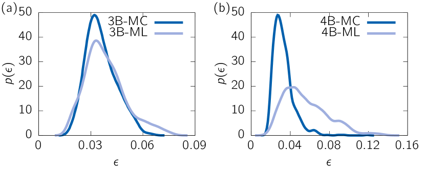
Figure 3: Distribution functions of confidence intervals, $p(\epsilon)$ (see Methods for definition), for both the out-of-sample predictions within the MC-sampled compounds and the ML-predicted compounds. (a) Trimers and (b) tetramers.

The extrapolation can also be seen in the projections of predicted transfer free energies, highlighting distinct coverages of sampled and predicted trimer compounds (Fig. 4). However, the main panels (a) and (b) display notable linear relations between transfer free energies—similar behavior is found for tetramers (Fig. S3). Importantly, similar linear relations had already been observed for CG unimers and dimers, highlighting thermodynamic relations for the transfer between different effective bulk environments Menichetti et al. (2017). We also argue that the ML models do not simply learn linear features, since we optimize independent models for the different predicted transfer free energies. The linear behavior displayed across both sampled and predicted compounds testifies to the robustness of the ML model, despite the extrapolation.

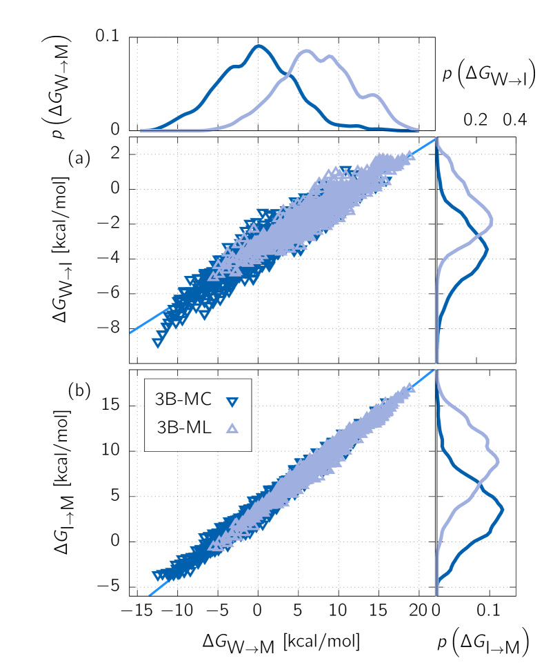
Figure 4: (a) Transfer free energies from water to interface $\Delta G_{\textup{W}\rightarrow\textup{I}}$ as a function of the compound’s water/membrane partitioning free energy, $\Delta G_{\textup{W}\rightarrow\textup{M}}$. The dark and light blue points depict corresponding quantities for trimers estimated from MC sampling (3B-MC) and the ML predictions (3B-ML), respectively. Linear fits highlight the molecular-weight dependence. (b) Transfer free energies from the interface to the membrane $\Delta G_{\textup{I}\rightarrow\textup{M}}$ as a function of the compound’s water/membrane partitioning free energy, $\Delta G_{\textup{W}\rightarrow\textup{M}}$. The coverages are projected down along a single variable on the sides. Error bars for 3B-MC are on par with the datapoint sizes (not shown).

The ML predictions also offer higher accuracy compared to simple linear fits: We selected a small set of 50 reference compounds spanning the entire dataset and measured the performance of the ML predictions and linear regression. The deviation of both predictions against reference alchemical transformations for each compound is shown in Fig. 5, displaying predictions for $\Delta G_{\textup{W}\rightarrow\textup{I}}$ and $\Delta G_{\textup{W}\rightarrow\textup{M}}$. We find a mean-absolute error (MAE) of 0.3 and 0.5 kcal/mol for the ML and linear fit, respectively. The linear regressions display equal but opposite errors between $\Delta G_{\textup{W}\rightarrow\textup{I}}$ and $\Delta G_{\textup{W}\rightarrow\textup{M}}$, by construction. The compounds are sorted according to the ML deviation of $\Delta G_{\textup{W}\rightarrow\textup{I}}$. Interestingly, this ranking of compounds shows no clear pattern: for instance, it only correlates weakly with hydrophobicity (21%). On the other hand hydrophobicity correlates much more strongly with the predictive variance (50%). While the latter naturally stems from the representation, the absence of correlation between ML deviation and hydrophobicity points at a more complex structure of the interpolation space (i.e., the CG chemical space)—a feature that will only worsen when learning atomistic compounds. Complementary information can be further probed from Fig. 5 by comparing the ML deviations between $\Delta G_{\textup{W}\rightarrow\textup{I}}$ and $\Delta G_{\textup{I}\rightarrow\textup{M}}$: we observe a correlation coefficient of 63% between the unsigned prediction errors. Training two independent ML models on identical subsets of chemical space leads to large correlations, further emphasizing the predominance of the interpolation space over the target property when learning.

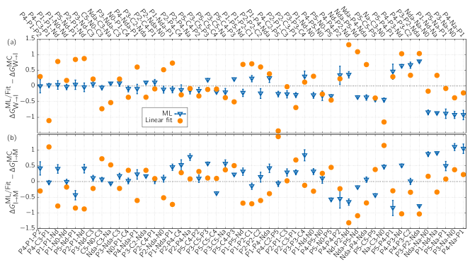
Figure 5: Deviations of the ML and linear-fit (“Fit”) predictions from reference alchemical transformations (“MC”) for (a) $\Delta G_{\textup{W}\rightarrow\textup{I}}$ and (b) $\Delta G_{\textup{I}\rightarrow\textup{M}}$. Error bars for the ML model display the 95% confidence intervals form the predictive variance. Compounds are sorted according to the ML prediction error for $\Delta G_{\textup{W}\rightarrow\textup{I}}$. Free energies displayed in units of kcal/mol.

A systematic coarse-graining of compounds in the GDB Fink and Reymond (2007) using Auto-Martini Bereau and Kremer (2015) was performed to identify small organic molecules that map to CG linear trimers. The algorithm is deterministic, such that it leads to a unique mapping from molecule to CG representation. We identified 1.36 million compounds, for which we can associate all three transfer free energies, $\Delta G_{\textup{W}\rightarrow\textup{M}}$, $\Delta G_{\textup{W}\rightarrow\textup{I}}$, and $\Delta G_{\textup{I}\rightarrow\textup{M}}$. We note that the sampled and predicted CG representations amount to similar numbers of compounds, such that the ML boosting introduced here offers an additional 0.8 million compounds to the database. The database is provided as supporting material for further data analysis.

IV Conclusions

The overwhelming size of chemical space naturally calls for statistical techniques to analyze it. A variety of data-driven methods such as quantitative structure-property relationships (QSPR) and ML models at large have been applied to chemical space Rupp et al. (2012); Faber et al. (2016); Bartók et al. (2017); Zhang et al. (2017). While sparse databases easily lead to overfitting Swift and Amaro (2013), a dense coverage can offer unprecedented insight Ramakrishnan et al. (2014). Here we rely on tools from statistical physics to ease the exploration of chemical space: the application of importance sampling guides us toward the subset of molecules that enhances a desired thermodynamic property. This approach is similar to recent generative ML models Sanchez-Lengeling and Aspuru-Guzik (2018), but without the a priori requirement for labeled training data.

In this work, we provide estimates of different transfer free energies (e.g., from water to the membrane interface, $\Delta G_{\textup{W}\rightarrow\textup{I}}$) for a large number of CG compounds. The combination of alchemical transformations with MC sampling motivates the calculation of free energies relative to the previous compound (e.g., $\Delta G^{A\rightarrow B}_{\textup{I}}$). Estimating the stability of compound $C_{i}$, sampled at the $i$-th step of an MC procedure, requires the summation of all previous free-energy contributions, all the way to the initial compound, for which we computed absolute free energies from umbrella sampling. Because each step in the MC procedure involves a free energy, there is a statistical error that is compounded during this reconstruction. We can take advantage of thermodynamic cycles to measure deviations from a net free energy of zero in a closed loop, and thus estimate this compounding of errors. Remarkably, we find deviations that are much smaller than the estimated statistical error of the alchemical transformations. This illustrates the robustness of estimating free energies at high throughput using an MC scheme.

A conceptually-appealing strategy to expand the MC-sampled distribution is through an ML model. Effectively we train an ML model on the MC samples and further boost the database with additional ML predictions. Unfortunately, the limited extrapolation behavior of kernel models means that accurate predictions can only be made for compounds similar to the training set. How similar is often difficult to estimate a priori. Similarity metrics are often based at the level of the ML’s input space—here the molecular representation. In Fig. 3 we used the predictive variance as a metric for the query sample’s distance to the training set Rasmussen (2004).

Beyond similarity in the ML’s input space via the predictive variance, we also consider the target properties directly. Our physical understanding of the problem offers a clear requirement on the transfer free energies, through the linear relationships shown in Fig. 4 Menichetti et al. (2017). As such, the thermodynamics of the system impose a physically-motivated constraint on the predictions. Rather than specific to each prediction, this constraint is global to the ensemble of data points. Satisfying it grounds our predictions within the physics of the problem, ensuring that we accurately expand the database.

Remarkably, we find that we can significantly expand our database—doubling it for trimers and a factor of 10 for tetramers (see SI)—while retaining accurate transfer free energies. Unlike conventional atomistic representations Faber et al. (2017), our ML model is encoded using a CG representation, such that compounds need only be similar at the CG level. This CG similarity is strongly compressed because ($i$) coarse-graining reduces the size of chemical space Menichetti et al. (2017), but also ($ii$) of a more straightforward structure-property link Menichetti et al. (2019). The latter is embodied by the additive contribution of bulk partitioning free energies for each bead, efficiently learning the molecular transfer free energy in more complex environments. All in all, backmapping (Fig. 1d) significantly amplifies the additional region of chemical space reached by the ML model. Our work highlights appealing aspects of bridging physics-based methodologies and coarse-grained modeling together with machine learning, offering increased robustness and transferability to explore significantly broader regions of chemical space.

V Supporting Information

The attached supporting information contains additional details on the optimization of thermodynamic cycles; the learning curves of the machine learning model; and results on linear tetramers. In addition, we provide databases for the transfer free energies of all trimers and tetramers, as well as atomistic-resolution compounds that map to trimers in a repository Hoffmann et al. (2019).

References

- Pyzer-Knapp et al. (2015) E. O. Pyzer-Knapp, C. Suh, R. Gómez-Bombarelli, J. Aguilera-Iparraguirre, and A. Aspuru-Guzik, Annual Review of Materials Research 45, 195 (2015).
- Jain et al. (2016) A. Jain, Y. Shin, and K. A. Persson, Nature Reviews Materials 1, 15004 (2016).
- Bereau et al. (2016) T. Bereau, D. Andrienko, and K. Kremer, APL Materials 4, 6391 (2016).
- von Lilienfeld (2018) O. A. von Lilienfeld, Angewandte Chemie International Edition 57, 4164 (2018).
- Curtarolo et al. (2013) S. Curtarolo, G. L. Hart, M. B. Nardelli, N. Mingo, S. Sanvito, and O. Levy, Nature materials 12, 191 (2013).
- Ghiringhelli et al. (2015) L. M. Ghiringhelli, J. Vybiral, S. V. Levchenko, C. Draxl, and M. Scheffler, Physical review letters 114, 105503 (2015).
- Ferguson (2017) A. L. Ferguson, Journal of Physics: Condensed Matter 30, 043002 (2017).
- Bereau (2018) T. Bereau, “Data-driven methods in multiscale modeling of soft matter,” in Handbook of Materials Modeling: Methods: Theory and Modeling, edited by W. Andreoni and S. Yip (Springer, 2018) pp. 1–12.
- Noid (2013) W. G. Noid, J. Chem. Phys. 139, 090901 (2013).
- Bereau and Kremer (2015) T. Bereau and K. Kremer, J. Chem. Theory Comput. 11, 2783 (2015).
- Periole and Marrink (2013) X. Periole and S.-J. Marrink, in Biomolecular Simulations (Springer, 2013) pp. 533–565.
- Menichetti et al. (2017) R. Menichetti, K. H. Kanekal, K. Kremer, and T. Bereau, The Journal of Chemical Physics 147, 125101 (2017).
- Menichetti et al. (2019) R. Menichetti, K. H. Kanekal, and T. Bereau, ACS Central Science 5, 290 (2019).
- Mongan et al. (2004) J. Mongan, D. A. Case, and J. A. McCammon, Journal of computational chemistry 25, 2038 (2004).
- Dahan et al. (2016) A. Dahan, A. Beig, D. Lindley, and J. M. Miller, Advanced drug delivery reviews 101, 99 (2016).
- Rasmussen (2004) C. E. Rasmussen, in Advanced lectures on machine learning (Springer, 2004) pp. 63–71.
- Bussi et al. (2007) G. Bussi, D. Donadio, and M. Parrinello, J. Chem. Phys. 126, 014101 (2007).
- Parrinello and Rahman (1981) M. Parrinello and A. Rahman, J. Appl. Phys. 52, 7182 (1981).
- Wassenaar et al. (2015) T. A. Wassenaar, H. I. Ingølfsson, R. A. Böckmann, D. P. Tieleman, and S. J. Marrink, J. Chem. Theory Comput. 11, 2144 (2015).
- Shirts and Chodera (2008) M. R. Shirts and J. D. Chodera, J. Chem. Phys. 129, 124105 (2008).
- Klimovich et al. (2015) P. V. Klimovich, M. R. Shirts, and D. L. Mobley, Journal of computer-aided molecular design 29, 397 (2015).
- Menichetti et al. (2018) R. Menichetti, K. Kremer, and T. Bereau, Biochemical and biophysical research communications 498, 282 (2018).
- Hagberg et al. (2008) A. Hagberg, P. Swart, and D. S Chult, Exploring network structure, dynamics, and function using NetworkX, Tech. Rep. (Los Alamos National Lab.(LANL), Los Alamos, NM (United States), 2008).
- Bastian et al. (2009) M. Bastian, S. Heymann, and M. Jacomy, in Third international AAAI conference on weblogs and social media (2009).
- Paton (1969) K. Paton, Communications of the ACM 12, 514 (1969).
- Avriel (2003) M. Avriel, Nonlinear programming: analysis and methods (Courier Corporation, 2003).
- Huang and Von Lilienfeld (2016) B. Huang and O. A. Von Lilienfeld, “Communication: Understanding molecular representations in machine learning: The role of uniqueness and target similarity,” (2016).
- Faber et al. (2018) F. A. Faber, A. S. Christensen, B. Huang, and O. A. von Lilienfeld, The Journal of Chemical Physics 148, 241717 (2018).
- Fink and Reymond (2007) T. Fink and J.-L. Reymond, J. Chem. Inf. Model. 47, 342 (2007).
- Rupp et al. (2012) M. Rupp, A. Tkatchenko, K.-R. Müller, and O. A. von Lilienfeld, Physical review letters 108, 058301 (2012).
- Faber et al. (2016) F. A. Faber, A. Lindmaa, O. A. von Lilienfeld, and R. Armiento, Physical review letters 117, 135502 (2016).
- Bartók et al. (2017) A. P. Bartók, S. De, C. Poelking, N. Bernstein, J. R. Kermode, G. Csányi, and M. Ceriotti, Science advances 3, e1701816 (2017).
- Zhang et al. (2017) L. Zhang, J. Tan, D. Han, and H. Zhu, Drug discovery today 22, 1680 (2017).
- Swift and Amaro (2013) R. V. Swift and R. E. Amaro, Chemical biology & drug design 81, 61 (2013).
- Ramakrishnan et al. (2014) R. Ramakrishnan, P. O. Dral, M. Rupp, and O. A. von Lilienfeld, Scientific data 1, 140022 (2014).
- Sanchez-Lengeling and Aspuru-Guzik (2018) B. Sanchez-Lengeling and A. Aspuru-Guzik, Science 361, 360 (2018).
- Faber et al. (2017) F. A. Faber, L. Hutchison, B. Huang, J. Gilmer, S. S. Schoenholz, G. E. Dahl, O. Vinyals, S. Kearnes, P. F. Riley, and O. A. von Lilienfeld, Journal of chemical theory and computation 13, 5255 (2017).
- Hoffmann et al. (2019) C. Hoffmann, R. Menichetti, K. H. Kanekal, and T. Bereau, “Drug-membrane transfer free energies for coarse-grained trimers and tetramers,” http://doi.org/10.5281/zenodo.2630488 (2019).