The Phase Space of $k$-Essence $f(R)$ Gravity Theory

Abstract

Among the remaining viable theories that can successfully describe the late-time era is the $k$-Essence theory and in this work we study in detail the phase space of $k$-Essence $f(R)$ gravity in vacuum. This theory can describe in a viable way the inflationary era too, so we shall study the phase space in detail, since this investigation may reveal general properties regarding the inflationary attractors. By appropriately choosing the dimensionless variables corresponding to the cosmological system, we shall construct an autonomous dynamical system, and we find the fixed points of the system. We focus on quasi-de Sitter attractors, but also to radiation and matter domination attractors, and study their stability. As we demonstrate, the phase space is mathematically rich since it contains stable manifold and unstable manifold. With regard to the inflationary attractors, these exist and become asymptotically unstable, a feature which we interpret as a strong hint that the theory has an inherent mechanism for graceful exit from inflation. We describe in full detail the underlying mathematical structures that control the instability of the inflationary attractors, and also we also address the same problem for radiation and matter domination attractors. The whole study is performed for both canonical and phantom scalar fields, and as we demonstrate, the canonical scalar $k$-Essence theory is structurally more appealing in comparison to the phantom theory, a result also demonstrated in the related literature on $k$-Essence $f(R)$ gravity.

I Introduction

The latest Planck constraints on cosmological parameters Aghanim:2018eyx , in conjunction with the striking observation of gravitational waves coming from binary neutron stars merging GBM:2017lvd , have significantly narrowed down the available models for the description of the late-time acceleration era, first observed in the late 90’s. Although most modified gravity models still can describe the late-time era in a concrete and viable way (see Nojiri:2017ncd ; Nojiri:2010wj ; Nojiri:2006ri ; Capozziello:2011et ; Capozziello:2010zz ; delaCruzDombriz:2012xy ; Olmo:2011uz for reviews), it is still important to have alternative descriptions that may generate a viable phenomenology. Among the remaining viable models that can describe the dark energy era, are the so-called $k$-Essence models Nojiri:2019dqc ; Chiba:1999ka ; ArmendarizPicon:2000dh ; ArmendarizPicon:1999rj ; Matsumoto:2010uv ; ArmendarizPicon:2000ah ; Chiba:2002mw ; Malquarti:2003nn ; Malquarti:2003hn ; Chimento:2003zf ; Chimento:2003ta ; Scherrer:2004au ; Aguirregabiria:2004te ; ArmendarizPicon:2005nz ; Abramo:2005be ; Rendall:2005fv ; Bruneton:2006gf ; dePutter:2007ny ; Babichev:2007dw ; Deffayet:2011gz ; Kan:2018odq that can also describe concretely the inflationary era. It is of crucial importance to find a model that can describe in a unified way the dark energy era and the inflationary era. In Ref. Nojiri:2019dqc such a theoretical framework was given in terms of $k$-Essence $f(R)$ gravity, and it was demonstrated that a viable inflationary era may be generated.

However, the results of Ref. Nojiri:2019dqc were strongly dependent on the specific model studied, and the true structure of the cosmological solutions must be further revealed. To this end in this work we shall study the full phase space of the $k$-Essence $f(R)$ gravity theory, using a simple $k$-Essence model. In order to do so we shall construct an autonomous dynamical system from the $k$-Essence $f(R)$ gravity theory, find the fixed points of the cosmological system and study their stability. We shall focus on cosmologies with physical interest, and particularly, quasi-de Sitter fixed points, matter domination and radiation domination fixed points. The dynamical system approach is a very rigid and formal way to extract interesting information about the dynamical evolution of the system and is very frequently used in cosmology Odintsov:2018zai ; Oikonomou:2019boy ; Odintsov:2018uaw ; Odintsov:2018awm ; Odintsov:2019ofr ; Boehmer:2014vea ; Bohmer:2010re ; Goheer:2007wu ; Leon:2014yua ; Guo:2013swa ; Leon:2010pu ; deSouza:2007zpn ; Giacomini:2017yuk ; Kofinas:2014aka ; Leon:2012mt ; Gonzalez:2006cj ; Alho:2016gzi ; Biswas:2015cva ; Muller:2014qja ; Mirza:2014nfa ; Rippl:1995bg ; Ivanov:2011vy ; Khurshudyan:2016qox ; Boko:2016mwr ; Odintsov:2017icc ; Granda:2017dlx ; Landim:2016gpz ; Landim:2015uda ; Landim:2016dxh ; Bari:2018edl ; Chakraborty:2018bxh ; Ganiou:2018dta ; Shah:2018qkh ; Oikonomou:2017ppp ; Odintsov:2017tbc ; Dutta:2017fjw ; Odintsov:2015wwp ; Kleidis:2018cdx .

In brief the results of our analysis are quite interesting since the vacuum $f(R)$ gravity phase space is strongly stable having stable quasi-de Sitter attractors, while the $k$-Essence $f(R)$ gravity has instabilities. Particularly, the phase space of the $k$-Essence $f(R)$ gravity has stable inflationary attractors, which asymptotically become unstable due to the existence of unstable manifolds in the phase space. Eventually, the unstable manifolds destabilize the dynamical system, and from a physical point of view this can be viewed as graceful exit from inflation. Similar results hold true for the radiation and matter domination fixed points. It is notable that we performed the analysis assuming that the scalar kinetic term corresponds to canonical scalar fields and to phantom scalar fields, with the canonical $k$-Essence theory showing the most physically appealing features. In addition, we find quite intriguing substructures in the phase space, of lower dimension in comparison to the original phase space. These substructures control eventually the stability of the dynamical system, these are the origin of stability. Finally, we also examine in brief the case that no scalar kinetic term is included, and similar results are found.

This paper is organized as follows: In section II we present in brief the essential features of the $k$-Essence $f(R)$ gravity model. In section III we construct the autonomous dynamical system of the $k$-Essence $f(R)$ gravity theory, by appropriately choosing the phase space variables, and we discuss when this dynamical system is strictly autonomous. In section IV we investigate in detail the phase space structure for $k$-Essence models with canonical or phantom scalar field kinetic term, while in section V, we study the phase space of the theory in the absence of a scalar field kinetic term. The conclusions along with a detailed discussion on the results, are presented in the end of the paper.

II The $k$-Essence $f(R)$ Gravity Theoretical Framework

The $k$-Essence $f(R)$ gravity theoretical framework belongs to the general $\tilde{f}(R,\phi,X)$ theory which has the following gravitational action,

$$S=\int d^{4}x\sqrt{-g}\big{(}\tilde{f}(R,\phi,X)+\mathcal{L}_{matter}\big{)}\,,$$ (1)

where $g^{\mu\nu}$ is the metric and $\sqrt{-g}$ its determinant. Also $R=g^{\mu\nu}R_{\mu\nu}$ is the Ricci scalar and $X=\dfrac{1}{2}\partial_{\mu}\phi\partial^{\mu}\phi$ is the kinetic term of the scalar field. Finally $\mathcal{L}_{matter}$ stands for the Lagrangian density of the matter fields. In our case we shall assume later on that no matter fields are present, so we will consider the vacuum case $\mathcal{L}_{matter}=0$.

For the $k$-Essence model we shall consider, the generalized function $\tilde{f}$ in the action has the following form,

$$\tilde{f}(R,\phi,X)=\dfrac{1}{2\kappa^{2}}f(R)+c_{1}X+G_{1}X^{2}\,;$$ (2)

this case leads to a specific category of $k$-Essence models, to which we shall refer to as “Model I” hereafter. Notice that depending on whether $c_{1}=1$ or $c_{1}=-1$, Model I describes a phantom scalar field or a canonical field respectively.

II.1 Equations of Motion of the $k$-Essence $f(R)$ Gravity Theory

Regardless of the specific form of $\tilde{f}(R,\phi,X)$ and the coupling (or non-coupling) of the kinetic $X$ term to the Ricci curvature, the equations of motion of the theory are derived, as usually, by varying the gravitational action of Eq. (1) with respect to the metric tensor, $g^{\mu\nu}$ and to the scalar field, $\phi$. The former case yields the field equations for the geometry of the spacetime, that is the generalized Einstein field equations, while the latter yields the evolution of the scalar field. We consider a flat Friedmann-Robertson-Walker (FRW) metric of the form,

$$ds^{2}=-dt^{2}+a(t)^{2}\sum_{1}^{3}(dx^{i})^{2}\,,$$ (3)

where $a(t)$ is the scale factor, and thus $H(t)=\dfrac{\dot{a}}{a}$ is the Hubble rate, and also we shall assume that no matter fields are present, so $\mathcal{L}_{matter}=0$.

Varying the gravitational action with respect to the metric tensor, we obtain,

$$-\dfrac{1}{2}\big{(}\tilde{f}(R)-R\tilde{F}(R)\big{)}-\dfrac{\kappa^{2}}{2}\tilde{f}_{X}\dot{\phi}^{2}-3H\dot{\tilde{F}}(R)=3H^{2}\tilde{F}(R)\,,$$

where $\tilde{F}(R)=\dfrac{\partial\tilde{f}}{\partial R}$ and $\tilde{f}_{X}=\dfrac{\partial\tilde{f}}{\partial X}$. As a result, since,

$$\ddot{\tilde{F}}(R)=-\dfrac{1}{2}\tilde{f}(R)+\tilde{F}(R)\Big{(}\dfrac{R}{2}-H^{2}\Big{)}-2H\dot{\tilde{F}}(R)\,,$$

the field equations for the $f(R)-X$ theory become

$$\ddot{\tilde{F}}(R)-H\dot{\tilde{F}}(R)-\dfrac{\kappa^{2}}{2}\tilde{f}_{X}\dot{\phi}^{2}=0\,.$$ (4)

Varying the gravitational action with respect to the scalar field, we obtain,

$$\dfrac{1}{a^{3}}\big{(}a^{3}\tilde{f}_{X}\dot{\phi}\big{)}^{\cdot}+\tilde{f}_{\phi}=0\,,$$

where $\tilde{f}_{\phi}=\dfrac{\partial\tilde{f}}{\partial\phi}$. Hence, the equation of motion for the scalar field is,

$$\tilde{f}_{X}\big{(}\ddot{\phi}+3H\dot{\phi}\big{)}+\dot{\tilde{f}}_{X}\dot{\phi}+\tilde{f}_{\phi}=0\,.$$ (5)

We can now specify the equations of motion for Model I given in Eq. (2). Since $\tilde{f}_{I}(R,\phi,X)=\dfrac{1}{2\kappa^{2}}f(R)+c_{1}X+G_{1}X^{2}$, we have,

$$\tilde{F}_{I}(R)=\dfrac{\partial\tilde{f}_{I}}{\partial R}=\dfrac{1}{2\kappa^{2}}F(R)\;\;\,,\;\;\;\tilde{f}_{I,\phi}=\dfrac{\partial\tilde{f}_{I}}{\partial\phi}=0\;\;\text{and}\;\;\;\tilde{f}_{I,X}=\dfrac{\partial\tilde{f}_{I}}{\partial X}=c_{1}+2G_{1}X\,.$$

where $c_{1}$ and $G_{1}$ are constants and can be viewed as free parameters for the models. Concerning $c_{1}$, its sign can indicate the type of scalar field cosmologies used, with $c_{1}=-1$ describing a canonical scalar field, while $c_{1}=1$ describing phantom scalar fields, and $c_{1}=0$ denoting the absence of a kinetic term, which is physically unmotivated, though we will examine this case as well. Consequently, the field equation becomes,

$$\ddot{F}(R)-H\dot{F}(R)-\kappa^{4}\dot{\phi}^{2}\big{(}c_{1}+2G_{1}X\big{)}=0\,,$$ (6)

and the evolution of the scalar field,

$$\big{(}c_{1}+2G_{1}X\big{)}\big{(}\ddot{\phi}+3H\dot{\phi})+2G_{1}\dot{X}\dot{\phi}=0\,.$$ (7)

Having the equations of motion at hand, we can introduce several dimensionless dynamical variables, and we shall construct an autonomous dynamical system, the phase space of which we shall extensively study.

III Setting up the Dynamical Model

In order to examine the cosmological implications and behavior of Model I (2), we shall investigate the mathematical structure of its phase space. In order to do so, we need to introduce appropriate dimensionless phase space variables which will constitute an autonomous dynamical system. Taking into account that in a flat FRW spacetime, we have,

$$R =6\dot{H}+12H^{2}\;\;\;\text{and}\;\;\;\dot{R}=24\dot{H}H+6\ddot{H}$$ (8)

$$X =-\dfrac{1}{2}\dot{\phi}^{2}\;\;\;\text{and}\;\;\;\dot{X}=-\dot{\phi}\ddot{\phi}\;\,,$$ (9)

we define the following five dimensionless phase space variables,

$$x_{1}=-\dfrac{\dot{F}}{HF}\;\;\,,\;\;\;x_{2}=-\dfrac{f}{6H^{2}F}\;\;\,,\;\;\;x_{3}=\dfrac{R}{6H^{2}}\;\;\,,\;\;\;x_{4}=\kappa^{2}\dot{\phi}\;\;\;\text{and}\;\;\;x_{5}=\dfrac{1}{\kappa^{2}H^{2}F}\,.$$ (10)

The first three of these variables are typical and have been defined as such in many similar $f(R)$ gravity phase space studies Odintsov:2017tbc , however the variables $x_{4}$ and $x_{5}$, are needed only in the $k$-Essence $f(R)$ gravity case. Their evolution will be studied by using the $e$-foldings number, $N$, defined as follows,

$$N=\int_{t_{in}}^{t_{fin}}H(t)dt\,,$$ (11)

where $t_{in}$ and $t_{fin}$ the initial and final time instances. The derivatives in respect to the $e$-foldings number are derived from the derivatives with respect to time, by using,

$$\dfrac{d}{dN}=\dfrac{1}{H}\dfrac{d}{dt}\,,\;\;\;\;\;\dfrac{d^{2}}{dN^{2}}=\dfrac{1}{H}\Big{(}\dfrac{d^{2}}{dt^{2}}-\dfrac{\dot{H}}{H}\dfrac{d}{dt}\Big{)}\,.$$

The equations governing the evolution of the five variables with respect to the $e$-foldings number are given from the equations of motion, expressed in terms of these variables.

Specifically, the evolution of $x_{1}$ with respect to the $e$-foldings number is given as,

$$\dfrac{dx_{1}}{dN}=\dfrac{1}{H}\dot{x}_{1}=-\dfrac{1}{H^{2}}\Bigg{(}\dfrac{\ddot{F}}{F}-\dfrac{\dot{H}}{H}\dfrac{\dot{F}}{F}-\Big{(}\dfrac{\dot{F}}{F}\Big{)}^{2}\Bigg{)}\,,$$ (12)

where, from the field equation (Eq. (6)), we derived,

$$-\dfrac{\ddot{F}}{H^{2}F}=-\dfrac{\dot{F}}{HF}-\dfrac{\kappa^{2}\dot{\phi}^{2}}{2H^{2}F}\big{(}c_{1}-G_{1}\dot{\phi}^{2}\big{)}=x_{1}-\dfrac{c_{1}-f_{D}x_{4}^{2}}{2}x_{4}^{2}x_{5}\,,$$

where $f_{D}=\dfrac{G_{1}}{\kappa^{4}}$ so that it becomes dimensionless, and also we used the definition of the variables,

$$\dfrac{\dot{H}}{H^{3}}\dfrac{\dot{F}}{F}=-x_{1}(x_{3}-2)\,,\;\;\;\;\;\;\Big{(}\dfrac{\dot{F}}{HF}\Big{)}^{2}=-x_{1}^{2}\,.$$

Consequently, the differential equation describing the evolution of $x_{1}$ is equal to,

$$\dfrac{dx_{1}}{dN}=-4+3x_{1}+x_{1}^{2}-x_{1}x_{3}+2x_{3}-\dfrac{c_{1}-f_{D}x_{4}^{2}}{2}x_{4}^{2}x_{5}\,.$$ (13)

The evolution of $x_{2}$ with respect to the $e$-foldings number is given as,

$$\dfrac{dx_{2}}{dN}=\dfrac{1}{H}\dot{x}_{2}=\dfrac{f}{6H^{3}F}\Big{(}-\dfrac{\dot{f}}{f}+\dfrac{\dot{H}}{H}+\dfrac{\dot{H}}{H}\Big{)}\,,$$ (14)

where, we used the definition of the phase space variables,

$$-\dfrac{\dot{f}}{6H^{3}F} =-\dfrac{\dot{R}}{6H^{3}}=-4(x_{3}-2)-m\;\;\,,$$

$$\frac{f}{6H^{2}F}\dfrac{\dot{H}}{H^{2}} =-2x_{2}(x_{3}-2)\,,\;\;\;\;\;\;\dfrac{f}{6H^{2}F}\dfrac{\dot{F}}{HF}=-x_{1}x_{2}\,,$$

where $m=-\dfrac{\ddot{H}}{H^{3}}$ is a dynamical variable of crucial importance. In our study, the dynamical system we shall derive will be autonomous only in the case that the variable $m$ is constant. Thus, the resulting differential equation describing the evolution of the variable $x_{2}$ is the following,

$$\dfrac{dx_{2}}{dN}=8-m+4x_{2}-4x_{3}+x_{1}x_{2}-2x_{2}x_{3}\,.$$ (15)

Accordingly, the evolution of $x_{3}$ with respect to the $e$-foldings number is given as follows,

$$\dfrac{dx_{3}}{dN}=\dfrac{1}{H}\dot{x}_{3}=\dfrac{R}{6H^{3}}\Big{(}\dfrac{\dot{R}}{R}-\dfrac{\dot{H}}{H}\Big{)}\,,$$ (16)

From the definition of the phase space variables, we obtain,

$$\dfrac{\dot{R}}{6H^{3}}=4\dfrac{\dot{H}}{H^{2}}+\dfrac{\ddot{H}}{H^{3}}=4(x_{3}-2)-m\;\;\;\text{and}\;\;\;\dfrac{R}{6H^{2}}\dfrac{\dot{H}}{H^{2}}=x_{3}(x_{3}-2)\,.$$

Consequently, the third differential equation is,

$$\dfrac{dx_{3}}{dN}=-8-m+8x_{3}-2x_{3}^{2}\,.$$ (17)

We should notice that this differential equation is independent from the rest, since the evolution of $x_{3}$ depends only on the variable itself and the parameter $m$. We will show later that this differential equation can be solved analytically for constant $m$.

The evolution of $x_{4}$ depends strongly on the value of the parameter $c_{1}$, in such a way that the differential equation governing the evolution has a completely different form when $c_{1}=0$. The evolution is given by,

$$\dfrac{dx_{4}}{dN}=\dfrac{1}{H}\dot{x_{4}}=\dfrac{\kappa^{2}\ddot{\phi}}{H}\,.$$ (18)

The second temporal derivative of the scalar field $\phi$ is derived from the equation of motion for the respective field, namely Eq. (7), whose form changes drastically with $c_{1}=0$. To demonstrate this, we substitute $X=-\dfrac{1}{2}\dot{\phi}^{2}$ and $\dot{X}=-\dot{\phi}\ddot{\phi}$ in Eq. (7) and solve it with respect to $\ddot{\phi}$, obtaining,

$$\ddot{\phi}=-3H\dot{\phi}\dfrac{c_{1}-f_{D}\kappa^{4}\dot{\phi}^{2}}{c_{1}-3f_{D}\kappa^{4}\dot{\phi}^{2}}\,.$$ (19)

When $c_{1}=0$, this expression is simplified to

$$\ddot{\phi}=-H\dot{\phi}\,.$$ (20)

In effect, we should consider two distinct forms of Model I, hereafter called “Model I$\alpha$” and “Model I$\beta$”, with the first describing the case $c_{1}\neq 0$ and the second describing the case $c_{1}=0$. The specific forms of the fourth differential equation are given below:

• For $c_{1}\neq 0$, the differential equation describing the evolution of the phase space variable $x_{4}$ becomes,

  $$\dfrac{dx_{4}}{dN}=\dfrac{3}{3f_{D}x_{4}^{2}-c_{1}}\big{(}x_{4}-x_{4}^{3}\big{)}\,.$$ (21)

  This differential equation resembles a non-linear oscillation, multiplied with a damping term. Similar to Eq. (17), the differential equation (21) is independent from all the other phase space variables and can be analytically integrated, as we will show shortly.

• For $c_{1}=0$, the differential equation describing the evolution of the phase space variable $x_{4}$ becomes,

  $$\dfrac{dx_{4}}{dN}=-x_{4}\,.$$ (22)

  This differential equation leads to a simple exponential evolution. Obviously, it is also independent and analytically integrated.

Finally, the evolution of the variable $x_{5}$ is given as,

$$\dfrac{dx_{5}}{dN}=\dfrac{1}{H}\dot{x}_{5}=-\dfrac{1}{\kappa^{2}H^{3}H}\Big{(}\dfrac{\dot{F}}{F}-2\dfrac{\dot{H}}{H}\Big{)}\,.$$ (23)

From the definition of the phase space variables, we may transform it to

$$\dfrac{dx_{5}}{dN}=\big{(}4-x_{1}+2x_{3}\big{)}x_{5}\,.$$ (24)

In conclusion, the dynamical system of the $k$-Essence $f(R)$ gravity model (2) corresponding to $c_{1}=-1$ and $c_{1}=1$ is the following,

$$\dfrac{dx_{1}}{dN}=-4+3x_{1}+x_{1}^{2}-x_{1}x_{3}+2x_{3}-\dfrac{c_{1}-f_{D}x_{4}^{2}}{2}x_{4}^{2}x_{5}\,,$$ (25)

$$\dfrac{dx_{2}}{dN}=8-m+4x_{2}-4x_{3}+x_{1}x_{2}-2x_{2}x_{3}\,,$$

$$\dfrac{dx_{3}}{dN}=-8-m+8x_{3}-2x_{3}^{2}\,,$$

$$\dfrac{dx_{4}}{dN}=\dfrac{3}{3f_{D}x_{4}^{2}-c_{1}}\big{(}x_{4}-x_{4}^{3}\big{)}\,,$$

$$\dfrac{dx_{5}}{dN}=\dfrac{1}{H}\dot{x}_{5}=\big{(}4-x_{1}+2x_{3}\big{)}x_{5}\,.$$

while the one corresponding to $c_{1}=0$ is equal to,

$$\dfrac{dx_{1}}{dN}=-4+3x_{1}+x_{1}^{2}-x_{1}x_{3}+2x_{3}-\dfrac{c_{1}-f_{D}x_{4}^{2}}{2}x_{4}^{2}x_{5}\,,$$ (26)

$$\dfrac{dx_{2}}{dN}=8-m+4x_{2}-4x_{3}+x_{1}x_{2}-2x_{2}x_{3}\,,$$

$$\dfrac{dx_{3}}{dN}=-8-m+8x_{3}-2x_{3}^{2}\,,$$

$$\dfrac{dx_{4}}{dN}=-x_{4}\,,$$

$$\dfrac{dx_{5}}{dN}=\dfrac{1}{H}\dot{x}_{5}=\big{(}4-x_{1}+2x_{3}\big{)}x_{5}\,.$$

In the following sections we shall extensively study the above dynamical systems in detail.

III.1 Friedmann Constraint and the Effective Equation of State

Considering all ingredients of the Universe as homogeneous ideal fluids, we may write down an effective equation of state (EoS) as follows,

$$w_{eff}=\dfrac{P}{\rho}\,,$$

where $\rho$ is the energy density of the matter fields and $P$ is the corresponding isotropic pressure. The effective barotrobic index, $w_{eff}$, is equal to,

$$w_{eff}=-1-\dfrac{2}{3}\dfrac{\dot{H}}{H^{2}}\,.$$ (27)

Given that the Ricci scalar in a FRW space time is $R=6\dot{H}+12H^{2}$, and, from the definitions of the phase space variables, $x_{3}=\dfrac{R}{6H^{2}}=\dfrac{\dot{H}}{H^{2}}+2$, we have

$$w_{eff}=-\dfrac{1}{3}(2x_{3}-1)\,.$$ (28)

The effective equation of state must be satisfied by all the fixed points of the dynamical systems (25) and (26), if these fixed points are physical.

By looking Eq. (28), it is apparent that $x_{3}$ determines the value of the EoS parameter $w_{eff}$ in the following way,

• If the Universe is in a de Sitter expansion phase, so that $w_{eff}=-1$, then $x_{3}=2$.

• If the Universe is dominated by effective curvature, so that $w_{eff}=-\dfrac{1}{3}$, then $x_{3}=1$.

• If the Universe is dominated by a pressure-free non-relativistic fluid (dust) so that $w_{eff}=0$, which corresponds to the matter-dominated era, then $x_{3}=\dfrac{1}{2}$.

• If the Universe is dominated by a relativistic fluids that $w_{eff}=\dfrac{1}{3}$, resulting to the radiation-dominated era, than $x_{3}=0$.

• If the Universe is dominated by stiff matter so that $w_{eff}=1$, then $x_{3}=-1$.

Another important relation that needs to be fulfilled by the model is the Friedman constraint, derived from the Friedman equation. Writing down the Friedman equation as,

$$-\dfrac{\dot{F}}{HF}-\dfrac{f}{6H^{2}F}+\dfrac{R}{6H^{2}}-\dfrac{\kappa^{2}}{2}\dfrac{f_{X}\dot{\phi}}{3H^{2}F}=1\,,$$ (29)

where the first three terms correspond to the curvature and the fourth to the scalar field, and by using the definition of the phase space variables, we obtain,

$$x_{1}+x_{2}+x_{3}-\dfrac{f_{X}}{6}x_{4}^{2}x_{5}=1\,.$$ (30)

Apparently, the constraint depends on the form of $\tilde{f}_{I}$. Since $f_{X}=c_{1}+2G_{1}X=c_{1}-f_{D}x_{4}^{2}$ and $c_{1}$ may come with two distinct versions of Model I, we have the following two cases:

• When $c_{1}\neq 0$, so we refer to Model I$\alpha$, then $f_{X}=c_{1}-f_{D}x_{4}^{2}$. The Friedman constraint for Model I$\alpha$ is the following,

  $$x_{1}+x_{2}+x_{3}-\dfrac{c_{1}-f_{D}x_{4}^{2}}{6}x_{4}^{2}x_{5}=1\,.$$ (31)

• In the special case of $c_{1}=0$, when we refer to Model I$\beta$, then $f_{X}=-f_{D}x_{4}^{2}$. Hence, the Friedman constraint for Model I$\beta$ becomes,

  $$x_{1}+x_{2}+x_{3}+\dfrac{f_{D}}{6}x_{4}^{4}x_{5}=1\,.$$ (32)

Having the above at hand, in the next sections we proceed to the analysis of the phase space structure for the $k$-Essence $f(R)$ gravity models we discussed in the previous sections.

As for parameter $m$, given the fact that it is merely the ratio of the second derivative over the cube of the Hubble rate, it is subject to the specific nature of the spacetime, that is of the specific nature of its matter content. Consequently, the values of $m$ are also very specific, if this is considered to be constant, which is our case. If we consider the three major phases of cosmic evolution, namely the quasi-de Sitter expansion, the matter-dominated era and the radiation-dominated era, we know that the Hubble rate has specific functional forms. Specifically, in the case of quasi-de Sitter expansion, and $H(t)=H_{0}-H_{i}t$, thus $m=0$. In the case of matter domination, $H(t)=\dfrac{2}{3t}$, and thus $m=-\dfrac{9}{2}$ and in the case of radiation domination, $H(t)=\dfrac{1}{2t}$, and thus $m=-8$. These values of $m$ are the values with major cosmological interest, hence the only values to be used hereafter.

III.2 Integrability of the Differential Equations for $x_{3}$ and $x_{4}$

As we noted earlier, two of the differential equations composing the dynamical systems (25) and (26), namely Eqs. (17) and (21) for Model I$\alpha$ and Eqs. (17) and (22) for Model I$\beta$, are independent from the other three, meaning that they do not contain any other phase space variables. Consequently, these first-order differential equations can be solved independently from the other, and it proves that these can be solved analytically. The independence of these equations, and by extent of the behavior of these two phase space variables, as well as the analytical solutions derived from them, can in fact explain the symmetries we observe later in the corresponding values of $x_{3}$ and $x_{4}$ in the equilibria, for all the cases we shall study (for any value of $m$ and $f_{D}$). They can also explain the stability properties these equilibrium values have, and the corresponding behavior of these variables independently of the others.

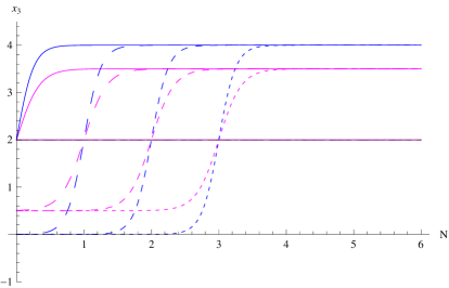
Figure 1: Analytical solutions derived for the differential equation (17) for different initial values (solid curves correspond to $N_{0}=0$, while thinner dashing corresponds to greater $N_{0}>0$), for $m=0$ (purple curves), $m=-\frac{9}{2}$ (magenta curves) and $m=-8$ (blue curves). The fast convergence to some equilibrium value is easily observable within 5 to 6 $e$-foldings.

Beginning with Eq. (17), the analytical solution is

$$x_{3}(N)=2-\dfrac{\sqrt{-2m}}{2}\tan\big{(}\sqrt{-2m}(N-N_{0})\big{)}\,,$$ (33)

where $N_{0}$ the e-foldings number corresponding to the initial time, i.e. the integration constant of Eq. (11) -usually chosen to be $N_{0}=0$ for simplicity, in the case of inflationary evolutions, since $t_{in}=t_{Pl}\simeq 5.39\;10^{-44}$ the initial moment for inflation. Assuming that $m=$constant, the differential equation (17) has no equilibrium points for $m>0$, and has one stable equilibrium point for $m=0$, $x_{3}^{*}=2$, and two equilibrium points for $m<0$, namely, $x_{3}^{*}=2\pm\dfrac{\sqrt{-2m}}{2}$. Of the two, $x_{3}^{*}<2$ is the unstable and $x_{3}^{*}>2$ is the stable equilibrium point. As a result, the analytical solutions for $m=0$ are $x_{3}=2$ for any $N$, and for $m<0$, the solutions converge rather fast to $x_{3}^{*}=2+\dfrac{\sqrt{-2m}}{2}$, with the rate of convergence depending on the initial conditions, typically on $N_{0}$. In Fig. 1 we have plotted the behavior of the variable $x_{3}$ for various values of the parameter $m$, namely for $m=0$ (quasi-de Sitter cosmologies), $m=-9/2$ (matter domination cosmology) and $m=-8$ (radiation domination cosmology).

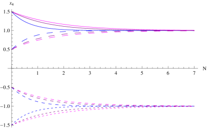
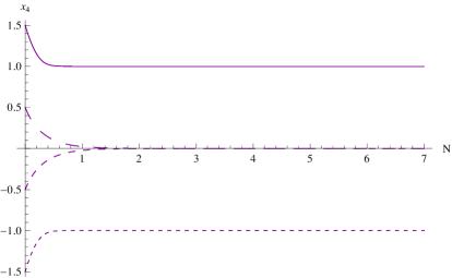
Figure 2: Analytical solutions derived for the differential equation (21) for different initial values (solid curves correspond to $N_{0}=0$, while thinner dashing corresponds to greater $N_{0}>0$), for $m=0$ (purple curves), $m=-\dfrac{9}{2}$ (magenta curves) and $m=-8$ (blue curves), and for both cases ($c_{1}=-1$ on the left, and $c_{1}=1$ on the right). The fast convergence is easily observable within $5$ to $6$ e-foldings.

As for Eq. (22), the solution is,

$$x_{4}=x_{4}(0)e^{-N}\,,$$ (34)

where $x_{4}(0)$ determined by the initial conditions. This solution converges asymptotically, though rapidly to $x_{4}^{*}=0$, which is proved to be the equilibrium value for $c_{1}=0$. It is remarkable that this convergence does not depend on any other parameter.

Finally, the analytical solution of the Eq. (21) is generally derived by means of inverse functions, so it is not possible to present it in closed form. It is however easy to plot it and extract the general behavior, and in Fig. 2 we present the behavior of $x_{4}$ for various $m$ and $c_{1}$. What is interesting about it, is that Eq. (21) has three equilibrium points, $x_{4}^{*}=0$, $x_{4}^{*}=-1$ and $x_{4}^{*}=-1$, with the first being unstable, and the other two stable for $c_{1}=-1$, while all are stable for $c_{1}=1$. Consequently, for $c_{1}=-1$ (canonical scalar cosmologies), the solutions with positive initial values converge rather fast to $x_{4}^{*}=1$ and those with negative initial values converge equally fast to $x_{4}^{*}=-1$. For $c_{1}=-1$ (cosmologies with canonical scalar fields), the solutions with initial values larger than unity converge to $x_{4}^{*}=1$, those with initial values smaller than $-1$ converge to $x_{4}^{*}=-1$ and, finally, those with initial values in the interval $[-1,1]$ converge to $x_{4}^{*}=0$. The rate of the convergence in any of these cases, depends on the choice of $f_{D}$. In Fig. 2 we present the behavior of the variable $x_{4}$ for various values of the parameter $m$ and $c_{1}$.

III.3 The three free parameters

One small comment is needed for the free parameters of the two models. Apart from $c_{1}$ that is inherent from the original theory, two more are included, defined as,

$$m=-\dfrac{\ddot{H}}{H^{3}}\,,\;\;\;\;\;\;f_{D}=\dfrac{G_{1}}{\kappa^{4}}\,.$$ (35)

Generally, the existence of one free parameter means that the corresponding dynamical system might pass through a number of bifurcations, accordingly to its dependence on this free parameter. The existence of more than one could make the situation far more complicated, with many more bifurcations occurring as different values can be assigned to all the free parameters. This essentially means that the structure of the phase space, and consequently the behavior of the system, may change. The existence of fixed points is questioned, their stability might be altered, attractors can appear and disappear, even chaotic behavior may arise.

Hopefully, in our case things are quite simpler, since our three free parameters are not so arbitrarily chosen actually. Due to the role they play in the model under study, they can be given very specific values. As a result, the parameter space is contained and certain aspects of the bifurcation analysis are similar. More specifically, $c_{1}$ can take just two values for Model I$\alpha$, that are $-1$ and $1$, and only one for Model I$\beta$, that is $0$; the reasons for this have been already explained earlier.

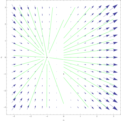
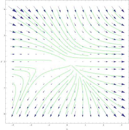
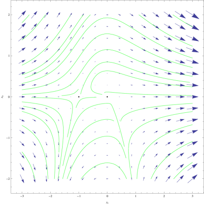
Figure 3: Several 2-d intersections of the phase space along the $x_{1}$ direction, for $c_{1}=-1$, $m=0$, $f_{D}=1$ and $x_{3}=2$. Blue arrows stand for the vector field, green curves for different solutions and black spots for viable equilibrium points.

The values for the parameter $m$ that will concern as were given earlier, which are $m=0$, $m=-9/2$ and $m=-8$ corresponding to quasi-de Sitter, matter domination and radiation domination cosmologies respectively. Finally, concerning the third parameter, $f_{D}$, no value specification is needed beforehand. It will prove that all values of $f_{D}>\dfrac{1}{3}$ are capable of securing at least one stable manifold in the phase space, thus ensuring some sort of stability. Given that the Friedman constraint must be fulfilled, a relation between the other two parameters and $f_{D}$ is given for each of the two distinct models.

IV The Phase Space of the Model I$\alpha$

Let us begin by examining the phase space of Model I$\alpha$, referring to a canonical scalar cosmology. The dynamical system is composed of Eqs. (13, 15, 17, 21 and 24) and it is subjected to constraint (31) and the effective barotropic index of Eq. (28). The qualitative examination of the phase space consists mainly of the location and characterization of the equilibrium points in the phase space.

In the course of this -and the next section- we shall refer to the vector field defined by differential equations (13), (15), (17), (21) and (24) as $\vec{V}(x_{1},x_{2},x_{3},x_{4},x_{5})$.

IV.1 Stability and Viability of the Equilibrium Points

Setting $\vec{V}(x_{1},x_{2},x_{3},x_{4},x_{5})=0$, we analytically derive sixteen critical points, many of them however come along with complex value in some of their coordinates. This complexity is mainly attributed to the parameter $m$, out of which we understand that the system is subject to a number of bifurcations, mainly due to the parameter $m$ shifting from positive to negative values.

If $m>0$, then all the critical points contain at least one complex value, so none of them can be an equilibrium point; this is not really a problem, since $m>0$ does not yield physically meaningful solutions. On the other hand, if $m=0$, then none of the critical points has a complex value and thus they all may be equilibrium points, however, only six of them exist due to coincidences. These eight equilibria are characterized by high degeneracy due to $m=0$ being the transcritical value in this bifurcation, and hence the eight equilibrium points exist in a transitionary state. Finally, if $m<0$, then six of the equilibrium points have complex values, hence the remaining ten are equilibrium points.

The value of $c_{1}$ does not play any role in the number of equilibrium points existing, neither does the value of $f_{D}$. However, either of them may alter the stability of the equilibria, by altering the eigenvalues of the linearized system which is,

$$\small\begin{pmatrix}\dfrac{d\xi_{1}}{dN}\\ \dfrac{d\xi_{2}}{dN}\\ \dfrac{d\xi_{3}}{dN}\\ \dfrac{d\xi_{4}}{dN}\\ \dfrac{d\xi_{5}}{dN}\end{pmatrix}=\begin{pmatrix}2x_{1}^{*}-x_{3}^{*}+3&0&2-x_{1}^{*}&x_{4}^{*}\left(2f_{D}(x_{4}^{*})^{2}-c_{1}\right)x_{5}^{*}&\dfrac{1}{2}x_{4}^{*\;2}\left(f_{D}x_{4}^{*\;2}-c_{1}\right)\\ x_{2}^{*}&x_{1}^{*}-2x_{3}^{*}+4&-2(x_{2}^{*}+2)&0&0\\ 0&0&8-4x_{3}^{*}&0&0\\ 0&0&0&-\dfrac{3\left(-3c_{1}x_{4}^{*\;2}+3f_{D}\left(x_{4}^{*\;2}+1\right)x_{4}^{*\;2}+c_{1}\right)}{\left(c_{1}-3f_{D}x_{4}^{*\;2}\right)^{2}}&0\\ -x_{5}^{*}&0&-2x_{5}^{*}&0&-x_{1}^{*}-2x_{3}^{*}+4\end{pmatrix}\begin{pmatrix}\xi_{1}\\ \xi_{2}\\ \xi_{3}\\ \xi_{4}\\ \xi_{5}\end{pmatrix}\,,$$ (36)

where $\{x_{i}^{*}\}$ indicate the values of the phase space variables in an equilibrium point and $\{\xi_{i}\}$ denote small linear perturbations of the phase space variables around them. It is proved, that in order to ensure structural stability for almost every equilibrium point, meaning at least one stable manifold, or at least one eigenvalue with negative real part in the linearized system, $f_{D}$ must have a lower boundary, respective to the $c_{1}$ value. Since $c_{1}$ may take only two possible values, $c_{1}=-1$ and $c_{1}=1$ respectively, $f_{D}$ has two lower boundaries arising from the first eigenvalue of Eqs. (36). These are

• For $c_{1}=-1$, that is in the case of canonical scalar field, $f_{D}>\dfrac{1}{3}$.

• For $c_{1}=1$, that is in the case of phantom scalar fields, $f_{D}>-\dfrac{1}{3}$.

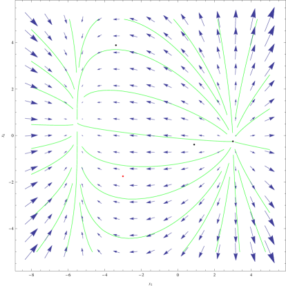
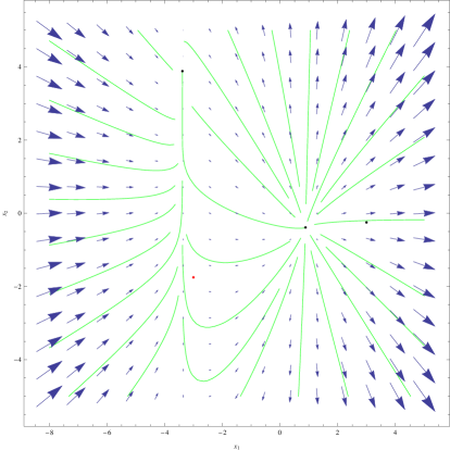
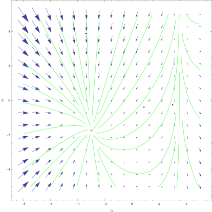
Figure 4: Several $x_{1}$-$x_{2}$ intersections of the phase space, for $c_{1}=-1$, $m=-\dfrac{9}{2}$, $f_{D}=3$ and $x_{4}=-1$. The first two plots correspond to $x_{3}=\dfrac{1}{2}$ (viable cosmological solutions), while the third correspond to $x_{3}=-\dfrac{7}{2}$ (non-viable cosmological solution). Blue arrows stand for the vector field, green curves for different solutions, black spots for viable equilibrium points and red spots for non-viable equilibrium points.

Furthermore, the values of $c_{1}$ and $f_{D}$ must also fulfill a specific relationship, in order to secure the viability of the majority of the equilibrium points, as the latter is encoded in the fulfillment of the Friedmann constraint, given in Eq. (31), and the effective equation of state, in Eq. (28). Beginning from the latter, we may easily rule out any equilibrium point that has a non-matching value for $x_{3}$. In that case, considering $m\leq 0$, only eight equilibrium points are deemed viable, regardless of the values of $c_{1}$ and $f_{D}$. Moving onto the fulfillment of the former, we demand that the Friedmann constraint is fulfilled by the eight equilibrium points at any case and for any possible value of $c_{1}$, $m$ and $f_{D}$ parameters. Thus we derive the following equation

$$f_{D}=1+6\dfrac{1-x_{1}^{*}-x_{2}^{*}-x_{3}^{*}}{x_{4}^{*\;4}x_{5}^{*}}=\dfrac{\left(3c_{1}\sqrt{-2m}+4m\right)}{\left(3\sqrt{-2m}+4m\right)}$$ (37)

taking into account the ruling out of two equilibria due to the effective equation of state for $m<0$. From Eq. (37), we are able to predetermine the value of the last parameter, $f_{D}$, for the specific values of the utilized for the other two, $c_{1}$ and $m$. However $c_{1}=1$ is obviously a pole for $f_{D}$, so in the cases of phantom scalar fields, $f_{D}$ is considered as a free parameter, chosen as $f_{D}=\dfrac{1}{2}$ for simplicity and without any lack of generality.

IV.1.1 Quasi-de Sitter Evolution for $c_{1}=-1$ and $m=0$

Given $c_{1}=-1$ and $m=0$, Eq. (37) is indeterminate, thus $f_{D}$ is indeed a free parameter. We assume that $f_{D}=1$ for any necessary calculation, without any lack of generality. Thus, the six equilibrium points are the following

$$\begin{split}&P_{1}(0,-1,2,-1,0)\;\;\;\,,\;\;\;P_{2}(0,-1,2,0,0)\;\;\;\,,\;\;\;P_{3}(0,-1,2,1,0)\;\;\,,\\ &P_{4}(-1,0,2,-1,0)\;\;\;\,,\;\;\;P_{5}(-1,0,2,0,0)\;\;\;\text{and}\;\;\;P_{6}(-1,0,2,1,0)\;\,.\end{split}$$ (38)

It is easy to check that all of them fulfill $w_{eff}=-1$ and the Friedmann constraint, thus all six of them are viable as cosmological attractor solutions.

Calculating the eigenvalues of the linearized system for these six equilibria, we come to the conclusion that five out of the six are structurally stable and more importantly asymptotically unstable, due to the presence of both positive and negative eigenvalues, with the sixth being the source of instability. Furthermore, the presence of at least one zero eigenvalue in each of them deems them as irregular and degenerate, a reasonable conclusion due to the transitional value of $m$ in the bifurcation precess (from positive $m$’s, where no equilibria exist, to negative $m$’s, where multiple equilibria arise).

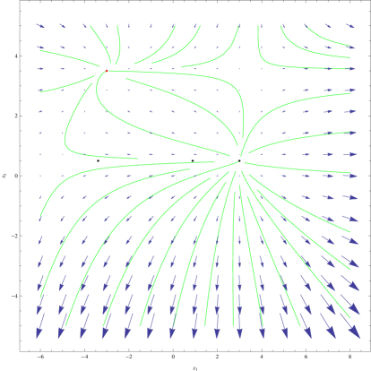
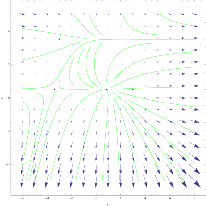
Figure 5: 2-d intersections of the phase space along the $x_{1}$ direction, for $c_{1}=-1$, $m=-\dfrac{9}{2}$, $f_{D}=3$ and $x_{4}=-1$; Both plots correspond to $x_{3}=\dfrac{1}{2}$ (viable cosmological solutions). Blue arrows stand for the vector field, green curves for different solutions, black spots for viable equilibrium points and red spots for non-viable equilibrium points.

More specifically:

• The $P_{1}$ and $P_{3}$ equilibrium points have one stable manifold in the direction of $v_{4}=(0,0,0,1,0)$, and one unstable in the direction of $v_{1,2}=(-1,1,0,0,0)$; the remaining three are transitionary.

• The $P_{2}$ equilibrium point has two unstable manifolds in the directions $v_{1,2}=(-1,1,0,0,0)$ and $v_{4}=(0,0,0,1,0)$; the remaining three are transitionary.

• The $P_{4}$ and $P_{6}$ equilibrium point have three stable manifolds in the directions $v_{1}=(1,0,0,0,0)$, $v_{2}=(0,1,0,0,0)$ and $v_{4}=(0,0,0,1,0)$, and one unstable in the direction of $v_{1,5}=\Big{(}\dfrac{1}{2},0,0,0,1\Big{)}$. The remaining one is transitionary. The stability in the directions $v_{1}$ and $v_{2}$ is degenerate, due to equal eigenvalues.

• The $P_{5}$ equilibrium point has two stable manifolds with degenerate stability, in the directions $v_{1}=(1,0,0,0,0)$ and $v_{2}=(0,1,0,0,0)$, and two unstable, $v_{4}=(0,0,0,1,0)$ and $v_{5}=(0,0,0,0,-1)$ and the remaining one is transitionary.

In Fig. 3, we present the behavior of the phase space variables close to the equilibrium points. It is easy to see that the attainment of an equilibrium is usually only along one or two dimensions of the phase space, or depends strongly on the initial conditions. Generally, the system seems to expand along the directions $x_{1}$ and $x_{5}$, exponentially leading these variables to infinity (or minus infinity).

The presence of asymptotic instability in the dynamical system, after some quasi-de Sitter attractors are reached, is particularly physically appealing. This is due to the fact that inflationary attractors are reached, and then the phase space structure of the $k$-Essence $f(R)$ gravity reaches some unstable manifolds (certain directions in the phase space), leading to the conclusion that the inflationary attractors become destabilized. This can be viewed as an inherent mechanism for graceful exit from inflation in the $k$-Essence $f(R)$ gravity theory. Thus combining the present results with those of Ref. Nojiri:2019dqc which indicated compatibility of $k$-Essence $f(R)$ gravity theory with the latest Planck data, this makes the theory particularly useful for describing inflationary dynamics.

IV.1.2 Matter-dominated Era: The Case $c_{1}=-1$ and $m=-\dfrac{9}{2}$

Let us focus in the case of having canonical scalar fields and matter domination cosmology, which is achieved by choosing $c_{1}=-1$ and $m=-\dfrac{9}{2}$. In effect, Eq. (37) yields $f_{D}=3$ so that the Friedmann constraint will be satisfied at least for those equilibria yielding $w_{eff}=0$. The ten equilibrium points in this case read,

$$\begin{split}&P_{1}\Big{(}3,-\dfrac{1}{4},\dfrac{1}{2},-1,-\dfrac{27}{4}\Big{)}\;\;\,,\;\;P_{2}\Big{(}-3,-\dfrac{7}{4},\dfrac{7}{2},-1,-\dfrac{27}{4}\Big{)}\;\;\;\,,\;\;\;P_{3}\Big{(}3,-\dfrac{1}{4},\dfrac{1}{2},1,-\dfrac{27}{4}\Big{)}\;\;\,,\;\;P_{4}\Big{(}-3,-\dfrac{7}{4},\dfrac{7}{2},1,-\dfrac{27}{4}\Big{)}\;\;\,,\\ &P_{5}\Big{(}-\dfrac{5+\sqrt{73}}{4},\dfrac{7+\sqrt{73}}{4},\dfrac{1}{2},-1,0\Big{)}\;\;\,,\;\;P_{6}\Big{(}-\dfrac{5+\sqrt{73}}{4},\dfrac{7+\sqrt{73}}{4},\dfrac{1}{2},0,0\Big{)}\;\;\,,\;\;P_{7}\Big{(}-\dfrac{5+\sqrt{73}}{4},\dfrac{7+\sqrt{73}}{4},\dfrac{1}{2},1,0\Big{)}\;\;\,,\\ &P_{8}\Big{(}-\dfrac{5-\sqrt{73}}{4},\dfrac{7-\sqrt{73}}{4},\dfrac{1}{2},-1,0\Big{)}\;\;\,,\;\;P_{9}\Big{(}-\dfrac{5-\sqrt{73}}{4},\dfrac{7-\sqrt{73}}{4},\dfrac{1}{2},0,0\Big{)}\;\;\text{and}\;\;P_{10}\Big{(}-\dfrac{5-\sqrt{73}}{4},\dfrac{7-\sqrt{73}}{4},\dfrac{1}{2},1,0\Big{)}\;\;\,.\end{split}$$ (39)

We can easily check that points $P_{2}$ and $P_{4}$ yield $w_{eff}=-2$ and do not satisfy the Friedmann constraint of Eq. (31). As a result, they correspond to non-viable cosmologies, however all other equilibrium points yield $w_{eff}=0$ and satisfy the Friedmann constraint.

In order to account for the stability of the equilibrium points, we calculate the eigenvalues of the linearized system (Eq. (36)). Again, all points but one turn to be structurally stable and asymptotically unstable, with at least one unstable manifold. The tenth point is proved unstable. More analytically,

• Points $P_{1}$ and $P_{3}$ have two stable and three unstable manifolds; two of the three unstable manifolds are degenerate due to the equality of the corresponding eigenvalues.

• Non-viable points $P_{2}$ and $P_{4}$ have four stable manifolds and one unstable; two of the four stable manifolds are degenerate as the equality of the corresponding eigenvalues suggest.

• Points $P_{5}$ and $P_{7}$ have three stable manifolds, in the directions of $v_{1,2}=(-1,1,0,0,0)$, $v_{2}=(0,1,0,0,0)$ and $v_{4}=(0,0,0,1,0)$, and two unstable.

• Point $P_{6}$ has two stable manifolds, in the directions of $v_{1,2}=(-1,1,0,0,0)$ and $v_{2}=(0,1,0,0,0)$, and three unstable manifolds.

• Points $P_{8}$ and $P_{10}$ have one stable manifold, in the direction of $v_{4}=(0,0,0,1,0)$, and four unstable manifolds.

• Point $P_{9}$ has five unstable manifolds, being an unstable node.

This behavior can partly be seen in Fig. 5 where we present the phase space structure in terms of some of the phase space variables.

IV.1.3 Radiation Dominated Era: The Case $c_{1}=-1$ and $m=-8$

Now let us consider the radiation domination cosmologies, in which case $m=-8$ and let us also investigate the case $c_{1}=-1$ which corresponds to canonical scalar fields. For $c_{1}=-1$ and $m=-8$, Eq. (37) yields $f_{D}=\dfrac{11}{5}$ so that the Friedmann constraint will be satisfied at least for those equilibria yielding $w_{eff}=\dfrac{1}{3}$. The ten equilibrium points in this case read,

$$\begin{split}&P_{1}(4,0,0,-1,-15)\;\;\;\,,\;\;\;P_{2}(-4,-2,4,-1,-15)\;\;\;\,,\;\;\;P_{3}(4,0,0,1,-15)\;\;\;\,,\;\;\;P_{4}(-4,-2,4,1,-15)\;\;\,,\\ &P_{5}(-4,5,0,-1,0)\;\;\;\,,\;\;\;P_{6}(-4,5,0,0,0)\;\;\;\,,\;\;\;P_{7}(-4,5,0,1,0)\;\;\,,\\ &P_{8}(1,0,0,0,-1,0)\;\;\;\,,\;\;\;P_{9}(1,0,0,0,0,0)\;\;\;\text{and}\;\;\;P_{10}(1,0,0,0,1,0)\,.\end{split}$$ (40)

We can easily check that points $P_{2}$ and $P_{4}$ yield $w_{eff}=-\dfrac{7}{3}$ and do not satisfy the Friedmann constraint of Eq. (31). As a result, they correspond to non-viable cosmologies. All other equilibrium points yield $w_{eff}=\dfrac{1}{3}$ and satisfy the Friedmann constraint.

As for the stability of the equilibrium points, the eigenvalues of the linearized system (Eq. (36)) for each of them reveal a complex and unstable nature, similar to the previous case. All points are accompanied by at least one unstable manifold and those providing the greater stability (four stable and one unstable manifolds) are the non-viable two, $P_{2}$ and $P_{4}$. More specifically,

• Points $P_{1}$ and $P_{3}$ have two stable and three unstable manifolds; two of the three unstable manifolds are degenerate due to the equality of the corresponding eigenvalues.

• Points $P_{2}$ and $P_{4}$ have four stable and one unstable manifolds; two of the four stable manifolds are degenerate as the equality of the corresponding eigenvalues suggest.

• Points $P_{5}$ and $P_{7}$ have two stable manifolds, in the directions $v_{1,2}=(-1,1,0,0,0)$ and $v_{4}=(0,0,0,1,0)$, and two degenerate unstable manifolds; they also have a transitionary one.

• Point $P_{6}$ has one stable manifold, in the direction $v_{1,2}=(-1,1,0,0,0)$ and three unstable, two of which are degenerate since their corresponding eigenvalues are equal; it also has a transitionary manifold corresponding to a zero eigenvalue.

• Points $P_{8}$ and $P_{10}$ have one stable manifold, in the direction $v_{4}=(0,0,0,1,0)$, and four unstable; two of the four unstable are degenerate, due to the equality of the corresponding eigenvalues.

• Point $P_{9}$ has five unstable manifolds, four of whom are pairwise degenerate, being a degenerate unstable node.

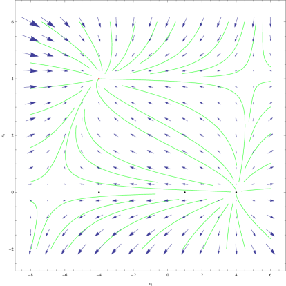
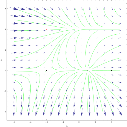
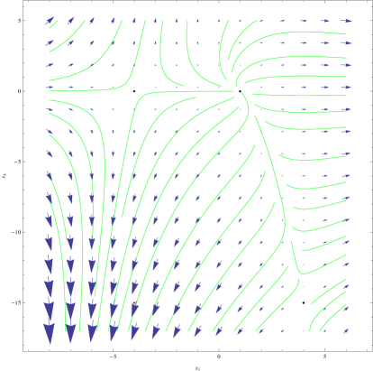
Figure 6: 2-d intersections of the phase space along the $x_{1}$ direction, for $c_{1}=-1$, $m=-8$, $f_{D}=3$. Blue arrows stand for the vector field, green curves for different solutions, black spots for viable equilibrium points and red spots for non-viable equilibrium points.

In Fig. 6 we present the behavior of some phase space variables, for $c_{1}=-1$, $m=-8$, $f_{D}=3$. It can be seen that the phase space has attractors, which eventually become destabilized.

IV.1.4 Quasi-de Sitter Evolution with Phantom Scalar Fields: The Case $c_{1}=1$ and $m=0$

Let us now consider quasi-de Sitter cosmologies, accompanied by phantom scalar fields. In this case $c_{1}=1$, the parameter $f_{D}$ is not determined by Eq. (37) and chosen as $f_{D}=\dfrac{1}{2}$; this value is sustained for all phantom scalar field cases. The six equilibrium points of the system when $c_{1}=1$ and $m=0$ are,

$$\begin{split}&P_{1}(0,-1,2,-1,0)\;\;\;\,,\;\;\;P_{2}(0,-1,2,0,0)\;\;\;\,,\;\;\;P_{3}(0,-1,2,1,0)\;\;\,,\\ &P_{4}(-1,0,2,-1,0)\;\;\;\,,\;\;\;P_{5}(-1,0,2,0,0)\;\;\;\text{and}\;\;\;P_{6}(-1,0,2,1,0)\,.\end{split}$$ (41)

The Friedmann constraint of Eq. (31) is generally satisfied and so is the effective equation of state, yielding $w_{eff}=-1$, in contrast to the phantom case, where some equilibria where unphysical.

Much similarly to the respective phantom scalar case studied earlier, the majority of the manifolds around the equilibrium points are transitionary, since $m=0$ is the indicative value for the bifurcation and the turning point for the sign of the eigenvalues. Furthermore, no clear stability is established for any point, with at least one unstable manifold being present in every one. Specifically,

• Points $P_{1}$, $P_{2}$ and $P_{3}$ have one stable manifold, in the direction of $v_{4}=(0,0,0,1,0)$, and one unstable, in the direction of $v_{1,2}=(-1,1,0,0,0)$; the remaining three are transitionary due to the zero corresponding eigenvalues.

• Points $P_{4}$, $P_{5}$ and $P_{6}$ have three stable manifolds, in the directions $v_{1}=(1,0,0,0,0)$ , $v_{2}=(0,1,0,0,0)$ and $v_{4}=(0,0,0,1,0)$, and one unstable manifold; the remaining one is accompanied by a zero eigenvalue, thus being transitionary.

The result is intriguing, since it seems that the canonical $k$-Essence $f(R)$ gravity theory is more physically appealing in comparison to the phantom scalar $k$-Essence $f(R)$ gravity. This result is of particular interest since it is aligned with the results of Ref. Nojiri:2019dqc indicating the same result, that the canonical scalar $k$-Essence $f(R)$ gravity is compatible with the Planck data, without extreme fine-tuning. In Fig. 7 we plot the behavior of several phase space variables for $c_{1}=1$, $m=0$, $f_{D}=\dfrac{1}{2}$. The instability we mentioned above is apparent in all plots.

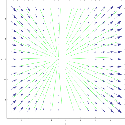
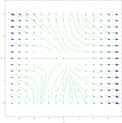
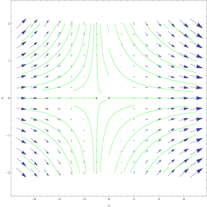
Figure 7: 2-d intersections of the phase space along the $x_{1}$ direction, for $c_{1}=1$, $m=0$, $f_{D}=\dfrac{1}{2}$ and $x_{3}=2$ (left and right plot), $x_{4}=-1$. Blue arrows stand for the vector field, green curves for different solutions and black spots for viable equilibrium points.

IV.1.5 Matter-dominated era with Phantom fields: $c_{1}=1$ and $m=-\dfrac{9}{2}$

Let us now consider matter dominated cosmologies with phantom scalar fields, so in this case $c_{1}=1$, $m=-\dfrac{9}{2}$ and $f_{D}=\dfrac{1}{2}$. The corresponding equilibrium points become ten and are the following,

$$\begin{split}&P_{1}\Big{(}3,-\dfrac{1}{4},\dfrac{1}{2},-1,18\Big{)}\;\;\,,\;\;P_{2}\Big{(}-3,-\dfrac{7}{4},\dfrac{7}{2},-1,18\Big{)}\;\;\;\,,\;\;\;P_{3}\Big{(}3,-\dfrac{1}{4},\dfrac{1}{2},1,18\Big{)}\;\;\,,\;\;P_{4}\Big{(}-3,-\dfrac{7}{4},\dfrac{7}{2},1,18\Big{)}\;\;\,,\\ &P_{5}\Big{(}-\dfrac{5+\sqrt{73}}{4},\dfrac{7+\sqrt{73}}{4},\dfrac{1}{2},-1,0\Big{)}\;\;\,,\;\;P_{6}\Big{(}-\dfrac{5+\sqrt{73}}{4},\dfrac{7+\sqrt{73}}{4},\dfrac{1}{2},0,0\Big{)}\;\;\,,\;\;P_{7}\Big{(}-\dfrac{5+\sqrt{73}}{4},\dfrac{7+\sqrt{73}}{4},\dfrac{1}{2},1,0\Big{)}\;\;\,,\\ &P_{8}\Big{(}-\dfrac{5-\sqrt{73}}{4},\dfrac{7-\sqrt{73}}{4},\dfrac{1}{2},-1,0\Big{)}\;\;\,,\;\;P_{9}\Big{(}-\dfrac{5-\sqrt{73}}{4},\dfrac{7-\sqrt{73}}{4},\dfrac{1}{2},0,0\Big{)}\;\;\text{and}\;\;P_{10}\Big{(}-\dfrac{5-\sqrt{73}}{4},\dfrac{7-\sqrt{73}}{4},\dfrac{1}{2},1,0\Big{)}\;\;\,.\end{split}$$ (42)

Of all of them, only five are viable, satisfying both the Friedmann constraint, Eq. (31), and the effective equation of state, Eq. (28). Points $P_{1}$ and $P_{3}$ satisfy the constraint, but yield $w_{eff}=-\dfrac{7}{3}$, while point $P_{7}$ satisfies the equation of state, but not the Friedman constraint. Finally points $P_{2}$ and $P_{4}$ satisfy neither constraint.

Concerning their stability, we again derive the eigenvalues of the linearized system of Eq. (36), and our analysis indicates that,

• Points $P_{1}$ and $P_{3}$ have two stable and three unstable manifolds; two of the latter are degenerate due to the equality of the corresponding eigenvalues.

• Points $P_{2}$ and $P_{4}$ have four stable and one unstable manifolds; two of the former are degenerate as the equality of the corresponding eigenvalues suggest.

• Points $P_{5}$ and $P_{7}$ have three stable manifolds, in the directions $v_{1,2}=(-1,1,0,0,0)$, $v_{2}=(0,1,0,0,0)$ and $v_{4}=(0,0,0,1,0)$, and two unstable.

• Point $P_{6}$ has four stable manifolds, in the directions $v_{1,2}=(-1,1,0,0,0)$, $v_{2}=(0,1,0,0,0)$, $v_{4}=(0,0,0,1,0)$ and $v_{5}=(0,0,0,0,1)$, and one unstable.

• Points $P_{8}$, $P_{9}$ and $P_{10}$ have one stable manifold, in the direction $v_{4}=(0,0,0,1,0)$, and four unstable manifolds.

The structure of the space is depicted in Fig. 8 for some of the phase space variables, for $c_{1}=1$, $m=-\dfrac{9}{2}$, $f_{D}=\dfrac{1}{2}$. In this case too, structural instabilities occur in the phase space, and this is a generic feature of the phantom scalar field $k$-Essence gravity.

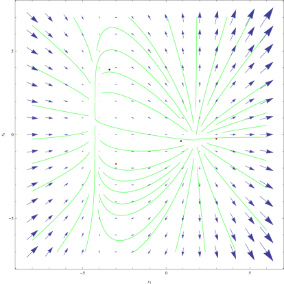
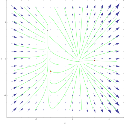
Figure 8: 2-d intersections of the phase space along the $x_{1}$ direction, for $c_{1}=1$, $m=-\dfrac{9}{2}$, $f_{D}=\dfrac{1}{2}$ and $x_{3}=\dfrac{1}{2}$ (corresponding to physically viable cosmological solutions). Blue arrows stand for the vector field, green curves for different solutions, black spots for viable equilibrium points and crimson and red spots for non-viable equilibrium points.

IV.1.6 Radiation Dominated Era with Phantom Scalar Fields: The Case $c_{1}=1$ and $m=-8$

Let us finally consider the case where phantom scalar fields are considered for radiation dominated cosmologies, in which case $c_{1}=1$, $m=-8$ and $f_{D}=\dfrac{1}{2}$. Our analysis indicates that the following ten equilibrium points exist,

$$\begin{split}&P_{1}(4,0,0,-1,32)\;\;\;\,,\;\;\;P_{2}(-4,-2,4,-1,32)\;\;\;\,,\;\;\;P_{3}(4,0,0,1,32)\;\;\;\,,\;\;\;P_{4}(-4,-2,4,1,32)\;\;\,,\\ &P_{5}(-4,5,0,-1,0)\;\;\;\,,\;\;\;P_{6}(-4,5,0,0,0)\;\;\;\,,\;\;\;P_{7}(-4,5,0,1,0)\;\;\,,\\ &P_{8}(1,0,0,0,-1,0)\;\;\;\,,\;\;\;P_{9}(1,0,0,0,0,0)\;\;\;\text{and}\;\;\;P_{10}(1,0,0,0,1,0)\,.\end{split}$$ (43)

Of these ten, the six satisfy both the Friedmann constraint of Eq. (31) and the effective equation of state (Eq. (28)), yielding $w_{eff}=0$, meaning that the phantom fields do not affect relativistic matter either. However, though points $P_{1}$ and $P_{3}$ yield $w_{eff}=-\dfrac{1}{3}$, they do not satisfy the constraint. Finally points $P_{2}$ and $P_{4}$ do satisfy neither of the constraints.

As for their stability, we may again check the eigenvalues of the linearized system of Eq. (36), and obtain the following results:

• Points $P_{1}$ and $P_{3}$ have two stable and three unstable manifolds; two of the latter are degenerate since the corresponding eigenvalues are equal.

• Points $P_{2}$ and $P_{4}$ have four stable and one unstable manifolds; of the former, two are degenerate as their equal eigenvalues suggest.

• Points $P_{5}$, $P_{6}$ and $P_{7}$ have two stable manifolds, in the directions $v_{1,2}=(-1,1,0,0,0)$ and $v_{4}=(0,0,0,1,0)$, and two degenerate unstable manifolds, due to the equality of their eigenvalues; the remaining one is transitionary, as the zero eigenvalue suggest.

• Points $P_{8}$, $P_{9}$ and $P_{10}$ have one stable manifold, in the direction $v_{4}=(0,0,0,1,0)$ and four unstable; two of the latter are proved degenerate due to the equality of the corresponding eigenvalues.

The above results can be clearly seen in Fig. 9, for $c_{1}=1$, $m=-8$, $f_{D}=\dfrac{1}{2}$.

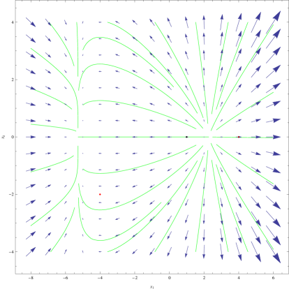
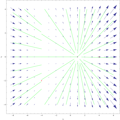
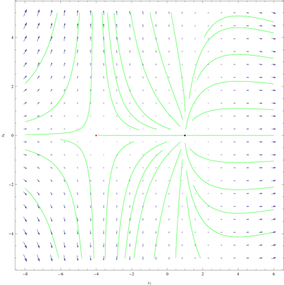
Figure 9: Several $x_{1}$-$x_{2}$ intersections of the phase space, for $c_{1}=1$, $m=-8$ and $f_{D}=\dfrac{1}{2}$. Blue arrows stand for the vector field, green curves for different solutions, black spots for viable equilibrium points and crimson and red spots for non-viable equilibrium points.

IV.2 A Possible $2-d$ Attractor

Very important information about a dynamical system arise from the divergence of its vector field, $\vec{V}(x_{1},x_{2},x_{3},x_{4},x_{5})$, which for the model at hand is equal to,

$$\vec{\nabla}\vec{V}=13+2x_{1}-9x_{3}+\dfrac{1}{f_{D}}\Big{(}-1-\dfrac{c_{1}-3f_{D}}{c_{1}-3f_{D}x_{4}^{2}}+\dfrac{2c_{1}(c_{1}-3f_{D})}{(c_{1}-3f_{D}x_{4}^{2})^{2}}\Big{)}\,.$$ (44)

Generally, a dynamical system is explosive if $\vec{\nabla}\vec{V}>0$, conservative if $\vec{\nabla}\vec{V}=0$, or dissipative if $\vec{\nabla}\vec{V}<0$, meaning that supervolumes of initial values are increasing, non-changing, or decreasing over time, respectively. In our case, the sign of the divergence of the flow changes, which means that the system is neither explosive, neither conservative, nor dissipative, but rather a mixture of all these depending on the phase space where the flow operates on the initial values.

According to the Poincaré-Bendixon theorem, the change of sign of the flow of a dynamical system indicates the existence of an attractor or a repeller in the phase, such as a stable or unstable limit cycle. The case of our dynamical system is similar, since the flow, $\vec{\nabla}\vec{V}$ turns zero along a specific three-dimensional curve, which is defined as follows,

$$x_{4}^{2}=\dfrac{3f_{D}+c_{1}\big{(}2f_{D}(13+2x_{1}-9x_{3})-3\big{)}-\sqrt{(3f_{D}-c_{1})\big{[}3f_{D}+c_{1}\big{(}3f_{D}-9+c_{1}(13+2x_{1}-9x_{3})\big{)}\big{]}}}{6f_{D}\big{(}f_{D}(13+2x_{1}-9x_{3})-1\big{)}}\,,$$ (45)

which is valid only when,

$$x{1}\neq\dfrac{9f_{D}x_{3}-13f_{D}+1}{2f_{D}}\,.$$

The curve defined in Eq. (45) can be further specified as follows:

• It becomes $x_{4}^{2}=\dfrac{-2\left(\sqrt{-4x_{1}+18x_{3}-23}+5\right)-2x_{1}+9x_{3}}{6x_{1}-27x_{3}+36}$ in the case of quasi-de Sitter expansion ($f_{D}=1$) and when a canonical scalar field is present ($c_{1}=-1$). The quantity on the right-hand side is generally real and positive for $x_{1}>\dfrac{1}{2}(9x_{3}-16)$, so $x_{4}$ takes realistic values across this curve. However, this curve is not proved to be an invariant under the flow of the system, thus it can not be categorized as an attractor.

• It becomes $x_{4}^{2}=-\dfrac{\sqrt{15}\sqrt{-8x_{1}+36x_{3}-49}+6x_{1}-27x_{3}+33}{9(6x_{1}-27x_{3}+38)}$ in the case of matter domination ($f_{D}=3$) and canonical scalar field ($c_{1}=-1$). Again, the quantity on the right-hand side is generally positive, so $x_{4}$ takes realistic values across the curve, for $x_{1}>\dfrac{1}{2}(9x_{3}-16)$.

• It becomes $x_{4}^{2}=-\dfrac{5\left(\sqrt{19}\sqrt{-88x_{1}+396x_{3}-533}+22x_{1}-99x_{3}+119\right)}{33(22x_{1}-99x_{3}+138)}$ in the case of radiation domination $\big{(}f_{D}=-\dfrac{11}{5}\big{)}$ and canonical scalar ($c_{1}=-1$). Once more, the quantity on the right-hand side is generally positive, so $x_{4}$ takes realistic values across the curve, for $x_{1}>\dfrac{1}{2}(9x_{3}-16)$.

• It becomes $x_{4}^{2}=\dfrac{-\sqrt{16x_{1}-72x_{3}+89}+4x_{1}-18x_{3}+23}{6x_{1}-27x_{3}+33}$ in the case of phantom scalar fields ($c_{1}=1$ and $f_{D}=\dfrac{1}{2}$). Here, the quantity on the right-hand side is generally negative, so $x_{4}$ would take non-realistic complex values across the curve. As a result, the attractor cannot exist in the case of phantom scalar fields.

The above results indicate that canonical $k$-Essence $f(R)$ gravity has more appealing physical features quantified in the presence of attractors in the phase space, for quite general values of the free parameters.

IV.3 Possible Issues in the Model

Before moving onto Model I$\beta$, we are bound to discuss a couple of issues arising for Model I$\alpha$, that lead to mathematically inconsistent or physically non-viable situations.

IV.3.1 Infinities for $c_{1}=1$

Beginning from Eq. (21), we can clearly see the existence of poles for $x_{4}^{2}=\pm\dfrac{c_{1}}{3f_{D}}$ and eventually for,

$$x_{4}=\pm\sqrt{\dfrac{c_{1}}{3f_{D}}}\,.$$ (46)

Of course, these poles are purely imaginary for $c_{1}=-1$ and are not so important in the case of canonical scalar fields. However, assuming $c_{1}=1$ and consequently $f_{D}>\dfrac{1}{3}$, the poles are purely real and appear as two straight hyperplanes along the phase space, in the form of,

$$x_{4}=\pm\sqrt{\dfrac{2}{3}}\,,$$

assuming $f_{D}=\dfrac{1}{2}$ as we did in the visualization of the vector field and the trajectories in the phase space. Close to these hyperplanes, the derivative of $x_{4}$ tends to infinity, and in effect the values of $x_{4}$ change rapidly towards infinity (or minus infinity) as well. This behavior is not natural and splits the phase space in three discrete and isolated subspaces, each of which has a specific sink. Any initial values of $x_{4}>\sqrt{\dfrac{2}{3}}$ tends to $x_{4}^{*}=1$ and those with initial values for $x_{4}<-\sqrt{\dfrac{2}{3}}$ tend to $x_{4}^{*}=-1$, while the initial conditions in $-\sqrt{\dfrac{2}{3}}<x_{4}<\sqrt{\dfrac{2}{3}}$ tend to $x_{4}^{*}=0$. As a result, when a phantom scalar field is present in contrast to the canonical scalar case, the state variable $x_{4}$ may tend to zero through a stable manifold . This indicates that $\dot{\phi}=0$, hence that the scalar field remains constant over time, is a stable solution for our model. This once more indicates the problematic physical situation that arises in the case where phantom scalars are used. This was also demonstrated in Ref. Nojiri:2019dqc where the phantom scalar $k$-Essence $f(R)$ gravity theory had to be extremely fine tuned in order for it to be viable and compatible with the Planck data.

V The Phase Space of the Model I$\beta$

Now let us turn our focus on the model I$\beta$, and we shall examine the phase space structure in the case $c_{1}=0$. The dynamical system describing such a cosmology is composed of Eqs. (13, 15, 17, 22 and 24) and it is subjected to constraint (32) and the effective barotropic index of Eq. (28).

This system is similar to the previous, with only one differential equation being altered namely Eq. (22), and some terms being simplified, due to $c_{1}=0$. As a result, many of our previous statements (e.g. the integrability of Eq. (17)) are still valid. However, some aspects of the system are different, since this version is much simpler, for example the number of critical points is reduced from sixteen to four.

V.1 Stability of the Equilibrium Points

Now let us investigate the stability of the fixed points by using an alternative approach by utilizing divergence field $\vec{V}(x_{1},x_{2},x_{3},x_{4},x_{5})$. Setting $\vec{V}(x_{1},x_{2},x_{3},x_{4},x_{5})=0$, we analytically derive four critical points, whose coordinates are functions of $m$. Consequently, the equilibria of the system are subjected to bifurcation, depending on the values of parameters $m$. More specifically, the four critical points have complex coordinates for $m>0$, so none of them is an equilibrium point, and two of them arise with real coordinates for $m\leq 0$, so these two are equilibrium points. Both of these equilibria fulfill both the Friedmann constraint (Eq. (32) and the effective equation of state, for each specific $m$, thus both equilibria are viable cosmological solutions. Since $m>0$ does not correspond to solutions with physical meaning, we shall remain with $m\leq 0$ and study the three cases with realistic behavior, with $m=0$ for the quasi-de Sitter expansion, $m=-\dfrac{9}{2}$ for the matter domination, and $m=-8$ for the radiation domination.

The linearized system around a miscellaneous equilibrium point $\{x_{i}^{*}\}$ is given as,

$$\small\begin{pmatrix}\dfrac{d\xi_{1}}{dN}\\ \dfrac{d\xi_{2}}{dN}\\ \dfrac{d\xi_{3}}{dN}\\ \dfrac{d\xi_{4}}{dN}\\ \dfrac{d\xi_{5}}{dN}\end{pmatrix}=\begin{pmatrix}2x_{1}^{*}-x_{3}^{*}+3&0&2-x_{1}^{*}&2f_{D}x_{4}^{3\;*}x_{5}^{*}&\dfrac{f_{D}x_{4}^{4\;*}}{2}\\ x_{2}^{*}&x_{1}^{*}-2x_{3}^{*}+4&-2(x_{2}^{*}+2)&0&0\\ 0&0&8-4x_{3}^{*}&0&0\\ 0&0&0&-1&0\\ -x_{5}^{*}&0&-2x_{5}^{*}&0&-x_{1}^{*}-2x_{3}^{*}+4\\ \end{pmatrix}\begin{pmatrix}\xi_{1}\\ \xi_{2}\\ \xi_{3}\\ \xi_{4}\\ \xi_{5}\end{pmatrix}\,,$$ (47)

where $\xi_{i}$ the linear perturbations of the phase space variables, $x_{i}$ around the equilibrium point.

Unlike the previous case, the $f_{D}$ parameter is not determined from the value of $m$ via the constraint. Thus it can be taken as a free parameter. Furthermore, the coordinates of the equilibrium points do not depending on $f_{D}$, and it is removed from the linearized system (since $x_{4}^{*}=x_{5}^{*}=0$) and by extent to the eigenvalues and eigenvectors of it close to the equilibrium points. For simplicity, and without any loss of generality, we set $f_{D}=1$ for any numerical calculation or plot we are about to conduct.

For a quasi-de Sitter evolution, $m=0$, so we may derive the following two equilibrium points,

$$P_{1}(-1,0,2,0,0)\;\;\;\text{and}\;\;\;P_{2}(0,-1,2,0,0)\,.$$ (48)

Using the linearized system from Eq. (47), we may reach to the following structure:

• Point $P_{1}$ has three degenerate stable manifolds, in the directions $v_{1}=(1,0,0,0,0)$, $v_{2}=(0,1,0,0,0)$ and $v_{4}=(0,0,0,1,0)$, and one unstable manifold, in the direction $v_{5}=(0,0,0,0,1)$; the remaining manifold, in direction $v_{1,2,3}=(-3,4,-1,0,0)$ is central transitionary, since the corresponding eigenvalue is zero.

• Point $P_{2}$ has one stable manifold, in direction $v_{4}=(0,0,0,1,0)$, and one unstable manifold, in the direction $v_{1,2}=(-1,1,0,0,0)$; the remaining three manifolds are central transitionary, since their eigenvalues equal zero.

In the same way, for the matter dominated era, in which case $m=-\dfrac{9}{2}$, the equilibrium points become,

Given $m=-\dfrac{9}{2}$, the equilibrium points become,

$$P_{1}\Big{(}-\dfrac{5+\sqrt{73}}{4},\dfrac{7+\sqrt{73}}{4},\dfrac{1}{2},0,0\Big{)}\;\;\;\text{and}\;\;\;P_{2}\Big{(}-\dfrac{5-\sqrt{73}}{4},\dfrac{7-\sqrt{73}}{4},\dfrac{1}{2},0,0\Big{)}\,.$$ (49)

From the linearized system from Eq. (47), we obtain the eigenvalues of each. Then the stability structure of the fixed points are as follows,

• Point $P_{1}$ has three stable manifolds, in the directions $v_{1,2}=(-1,1,0,0,0)$, $v_{2}=(0,1,0,0,0)$ and $v_{4}=(0,0,0,1,0)$, and two unstable manifolds.

• Point $P_{2}$ has two stable manifolds, in directions $v_{4}=(0,0,0,1,0)$ and $v_{5}=(0,0,0,0,1)$, and three unstable manifolds.

Finally, for the radiation domination era, given $m=-8$, the equilibrium points are,

$$P_{1}(-4,5,0,0,0)\;\;\;\text{and}\;\;\;P_{2}(1,0,0,0,0)\,.$$ (50)

From the linearized system from Eq. (47), the stability of each is obtained as follows,

• Point $P_{1}$ has two degenerate stable manifolds, in the directions $v_{1,2}=(-1,1,0,0,0)$ and $v_{2}=(0,1,0,0,0)$, and two degenerate unstable manifolds; the remaining one yields a zero eigenvalue, being a central transitionary.

• Point $P_{2}$ has one stable manifold, in directions $v_{4}=(0,0,0,1,0)$, and four unstable manifolds; two of the latter have equal eigenvalues, being degenerate.

Thus in the $c_{1}=0$ case, certainly the phase space contains some stable attractors, and an interesting property of the phase space is analyzed in the next section.

V.2 A $1-d$ attractor

As in the previous model, the flow of the system, defined as $\vec{\nabla}\vec{V}$ does not maintain its sign, thus it is impossible to define the system as conservative, dissipative or explosive. More specifically,

$$\vec{\nabla}\vec{V}=18+2x_{1}-9x_{3}\,,$$ (51)

that changes sign astride a straight hypersurface. It is very interesting that the flow of the system does not depend on the variables $x_{2}$, $x_{4}$ and $x_{5}$ and on the parameters $m$ and $f_{D}$, thus the line is not subject to bifurcations as the position and stability of the equilibrium points do. Demanding that $\vec{\nabla}\vec{V}=0$, we find that the equation of this hypersurface (actually it is a line) is as follows,

$$x_{1}=-\dfrac{9}{2}(2-x_{3})\,.$$ (52)

This supersurface is fully determined as a function of the $e$-foldings number, $N$, since $x_{3}$ is given as an analytic solution of Eq. (17). Thus, Eq. (52) provides us with an analytic solution for $x_{1}$ as well, in the form,

$$x_{1}(N)=-7-\dfrac{9\sqrt{-2m}}{4}\tan\big{(}\sqrt{-2m}(N-N_{0})\big{)}\,.$$ (53)

Solutions of Eq. (13) are thus driven by solutions of Eq. (17), and by extent they are attracted towards the value,

$$x_{1}^{\star}=-\dfrac{9\sqrt{2m}}{4}\tan\left(\sqrt{2m}\right)\,.$$ (54)

This values does not correspond to an equilibrium point, except for the quasi-de Sitter evolution case ($m=0$). Several analytic solutions of Eq. (13) that correspond to the $1-d$ attractor existing for $c_{1}=0$ are presented in Fig. 10.

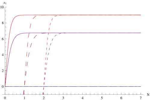
Figure 10: Analytic solutions of Eq. (13) that correspond to the $1-d$ attractor existing for $c_{1}=0$. Blue curves stand for $m=0$, purple curves for $m=-\dfrac{9}{2}$ and red ones for $m=-8$; the solid curves denote initial conditions for $N_{0}=0$, while dashing becomes thinner as $N_{0}>0$ grows.

One should also give notice to the strong intermingling of the $f(R)$ function and its rate of change, $\dot{f}(R)$, with the curvature. If we substitute the variables $x_{1}$ and $x_{3}$ from their definitions (Eq. (10), to the Eq. (52), we obtain the following relation

$$\dfrac{\dot{f}}{f}=\dfrac{R}{6H}-9H\,.$$ (55)

Thus even the case $c_{1}=0$ provides us with a rich phase space structure, although this case is less physically interesting in comparison to the other two cases analyzed in the previous sections.

VI Conclusions and Discussion of the Results

In this paper we thoroughly examined the phase space of a simple $k$-Essence $f(R)$ gravity theory. We studied both the cases that the $k$-Essence field consists of a phantom or a canonical scalar field. We analyzed two models focusing on cosmological solutions with physical interest and we emphasized our study on finding physically interesting fixed points in the theory. After appropriately choosing the phase space variables, we constructed an autonomous dynamical system, with the only deviation from being autonomous contained in the parameter $m=-\frac{\ddot{H}}{H^{3}}$. It turned out that for cosmologically interesting cases, the parameter $m$ takes constant values, and the dynamical system is rendered autonomous. Specifically for $m=0$ it describes a quasi-de Sitter cosmology, for $m=-\frac{9}{2}$ it describes a matter dominated cosmology and finally for $m=-8$ it describes a radiation domination era.

Proceeding to the analysis of the dynamical system, we isolated three major cases, identified as $c_{1}=-1$ which corresponds to a canonical scalar field, $c_{1}=0$, which implies the absence of a kinetic term for the scalar field, and $c_{1}=1$ which corresponds to phantom field cosmologies. These total nine physical situations can be studied as different static versions of a specific system. However, they can be studied as three different systems (concerning the values of $c_{1}$) that are subject to a bifurcation (concerning the values of $m$). In this sense, we may extracted some interesting results, summarized below.

First of all, given that $c_{1}=-1$ or $c_{1}=1$, the bifurcation of $m$ from positive values to zero creates six equilibrium points, and from zero to negative values to further four; two of these four in the cases of canonical scalar fields, and all four in the cases of phantom fields, are non-viable equilibria, since they do not fulfill the Friedmann constraint and/or the effective equation of state for the specific matter fields content. Furthermore, the appearance of equilibrium points occurs in such a way that specific symmetries are present and easily observed in the values of $x_{1}$ and $x_{2}$ phase space variables, even more in the values of $x_{4}$ and $x_{5}$ phase space variables. Taking into account the definitions of the phase space variables, the symmetries observed in $x_{1}$ and $x_{2}$ are symmetries concerning the specific form of the $f(R)$ function; on the other side, the symmetries observed in $x_{4}$ correspond to the behavior of the scalar field, $\phi$. Finally, $x_{5}$ has a usual equilibrium value at zero, which denotes an infinite rate of increase (or decrease) for either the Hubble rate, or the $f(R)$ function. Intriguingly enough, the equilibrium points for which $x_{5}^{*}\neq 0$ are usually the non-viable points for $m<0$. Furthermore, two of these are always found asymptotically stable in four directions. The equilibria for which $x_{5}^{*}=0$ are usually found to be asymptotically unstable, at least in directions such as $x_{5}$. This is the main source of instability in the quasi-de Sitter case and quantifies mathematically the ability of the present theory to generate the graceful exit from inflation.

The four emerging (and partially non-viable) equilibrium points are conceived as two pairs, mirrored on $x_{4}=0$, which denotes the constancy of the scalar field, since four of their coordinates are exactly the same and the fifth (the $x_{4}^{*}$) takes respectively the values $-1$ and $1$. In fact the stability of two mirrors the stability of the other two, qualitatively (the number of stable manifolds) and quantitatively (the direction of the stable and unstable manifolds). The stability of each isolated equilibrium is generally preserved through the bifurcations, with one important note: moving from $m=0$ to $m<0$, the number of central transitionary manifolds decreases and stable manifolds replace them.

The remaining six (always viable) equilibrium points can also be perceived as two groups of three, mirrored on $x_{4}=0$, with all other coordinates being equal (in each group), and $x_{4}$ taking the values $-1$, $0$ and $1$. The stability of each group seems correlated, with points with relatively more stable manifolds being grouped together and those with fewer stable manifolds alike. In the same manner, the equilibria of a group with $x_{4}^{*}=0$ are proved to be relatively more unstable that the other two. This peculiar symmetry reveals a fundamental problem in the case of $\phi=\text{const.}$, that repels solutions towards $x_{4}^{*}=-1$ or $x_{4}^{*}=1$. The gradual disappearance of central transitionary manifolds as $m$ moves from zero to negative values is observed here as well. Following the typical scheme for the evolution of the Universe, some of the central manifolds are preserved when $m=-8$ (radiation-dominated era) but are completely absent for $m=-\dfrac{9}{2}$, proving that the values of parameter $m$ are not decreasing linearly and uniformly.

Given the degenerate case of $c_{1}=0$, the number of equilibrium points is narrowed down to only two. Here $x_{4}^{*}=x_{5}^{*}=0$ always. Still, both equilibria are proved viable according to the Friedmann constraint and the effective equation of state. The two equilibrium points generally preserve their stable manifolds as the values of $m$ move from $0$ to $-\dfrac{9}{2}$ and $-8$. The first of these points for which $x_{1}^{*}<x_{2}^{*}$, has more stable manifolds. Once more, the transition from $m=0$ to $m=-8$ does not completely transform the central transitionary manifolds to stable ones, as it happens when $m=-8$ changes to $m=-\dfrac{9}{2}$. The standard model for cosmic evolution is somehow present in this phase transition, concerning the stability of the equilibria.

Second, a possible attractor appears in all three major cases. For $c_{1}=0$ the attractor is a 1-d hypersurface, that connects the $x_{1}$ and $x_{3}$ phase space variables and does not depend on any parameter values. When $c_{1}=-1$ or $c_{1}=1$, the attractor is a 1-d hypersurface, that connects the $x_{1}$, $x_{3}$ and $x_{4}$ phase space variables and depends strongly on the choice of $f_{D}$ and $c_{1}$. However, its complexity is such that its existence is not guaranteed. Interestingly, in any of the above cases the possible attractor connects the rate of change of the $f(R)$ function (from the $x_{1}$ variable) to the curvature scalar $R$ (from the $x_{3}$ variable) and to the rate of change of the scalar field (from the $x_{4}$ variable). However, the two of these variables do not only correspond to specific symmetries in the model, as observed in the equilibrium points, but also determine the effective equation of state and the Friedmann constraint respectively. Furthermore, their dynamical equations are separated from the other variables in a certain way, leading to their integrability and triviality.

Finally, if we observe this separation of Eqs. (17) and (21 or 22) from the other three and analyze their integrability, we come to the easy result that both $x_{3}$ and $x_{4}$, or with other words the scalar curvature and the rate of change of the scalar field, are trivially and independently evolving towards an equilibrium value. As long as the scalar field is concerned, the attained equilibrium value(s) are normal and correspond to viable cosmological solutions. When the scalar curvature is taken into account, we observe that aside from the case of quasi-de Sitter evolution, the equilibrium attained does not correspond to the barotropic index of the specific matter fields content, and thus relates to non-viable cosmological solutions.

As a consequence of the above, the system is characterized by two extremely different states. On the one hand, an asymptotic instability is observed in almost every equilibrium point that was noted. This instability is further amplified, if we take into consideration that the greater stability resolves around non-viable cosmological solutions. Concerning quasi-de Sitter fixed points, this asymptotical instability after an attractor is reached, may be viewed as an inherent mechanism for graceful exit in the $k$-Essence $f(R)$ gravity theory.

On the other hand, a high degeneracy is easy to be noted, given the fact that many equilibrium points emerge, and have specific symmetries in their coordinates, as well as the eigenvalues and eigenvectors of the linear perturbations, that characterize their stability. Also two of the dynamical equations are separated from the rest and integrated, resulting to trivial solutions for $x_{3}$ and $x_{4}$. The third state variable, $x_{1}$, is (in some cases) strongly interconnected with the $x_{3}$ and $x_{4}$ via an attractor, and thus its behavior is analytically traced and found diverging from the noted equilibria (viable or not). Finally, many of the stable or unstable manifolds around the equilibrium points are proved degenerate.

A possible resolution of this degeneracy would be the transformation of the system into another and the subsequent reduction of its dimensions from five to four, or ever three. This would expel the degeneracy and would give us a clearer picture for the general behavior of the system, under the aforementioned bifurcations. However, the fundamental instabilities of the system are not expected to alter following such a transformation. This issue is more probably an issue of the theoretical framework out of which the models were derived, rather than of the specific dynamical system, indicating for the quasi-de Sitter fixed points that the final attractors are unstable asymptotically and thus this is a strong hint that the theory possesses an internal structure that allows a graceful exit from inflation.

References

- (1) N. Aghanim et al. [Planck Collaboration], arXiv:1807.06209 [astro-ph.CO].
- (2) B. P. Abbott et al. [LIGO Scientific and Virgo and Fermi GBM and INTEGRAL and IceCube and IPN and Insight-Hxmt and ANTARES and Swift and Dark Energy Camera GW-EM and DES and DLT40 and GRAWITA and Fermi-LAT and ATCA and ASKAP and OzGrav and DWF (Deeper Wider Faster Program) and AST3 and CAASTRO and VINROUGE and MASTER and J-GEM and GROWTH and JAGWAR and CaltechNRAO and TTU-NRAO and NuSTAR and Pan-STARRS and KU and Nordic Optical Telescope and ePESSTO and GROND and Texas Tech University and TOROS and BOOTES and MWA and CALET and IKI-GW Follow-up and H.E.S.S. and LOFAR and LWA and HAWC and Pierre Auger and ALMA and Pi of Sky and DFN and ATLAS Telescopes and High Time Resolution Universe Survey and RIMAS and RATIR and SKA South Africa/MeerKAT Collaborations and AstroSat Cadmium Zinc Telluride Imager Team and AGILE Team and 1M2H Team and Las Cumbres Observatory Group and MAXI Team and TZAC Consortium and SALT Group and Euro VLBI Team and Chandra Team at McGill University], Astrophys. J. 848 (2017) no.2, L12 doi:10.3847/2041-8213/aa91c9 [arXiv:1710.05833 [astro-ph.HE]].
- (3) S. Nojiri, S. D. Odintsov and V. K. Oikonomou, Phys. Rept. 692 (2017) 1 doi:10.1016/j.physrep.2017.06.001 [arXiv:1705.11098 [gr-qc]].
- (4) S. Nojiri and S. D. Odintsov, Phys. Rept. 505 (2011) 59 doi:10.1016/j.physrep.2011.04.001 [arXiv:1011.0544 [gr-qc]].
- (5) S. Nojiri and S. D. Odintsov, eConf C 0602061 (2006) 06 [Int. J. Geom. Meth. Mod. Phys. 4 (2007) 115] doi:10.1142/S0219887807001928 [hep-th/0601213].
- (6) S. Capozziello and M. De Laurentis, Phys. Rept. 509 (2011) 167 doi:10.1016/j.physrep.2011.09.003 [arXiv:1108.6266 [gr-qc]].
- (7) V. Faraoni and S. Capozziello, Fundam. Theor. Phys. 170 (2010). doi:10.1007/978-94-007-0165-6
- (8) A. de la Cruz-Dombriz and D. Saez-Gomez, Entropy 14 (2012) 1717 doi:10.3390/e14091717 [arXiv:1207.2663 [gr-qc]].
- (9) G. J. Olmo, Int. J. Mod. Phys. D 20 (2011) 413 doi:10.1142/S0218271811018925 [arXiv:1101.3864 [gr-qc]].
- (10) S. Nojiri, S. D. Odintsov and V. K. Oikonomou, Nucl. Phys. B 941 (2019) 11 doi:10.1016/j.nuclphysb.2019.02.008 [arXiv:1902.03669 [gr-qc]].
- (11) T. Chiba, T. Okabe and M. Yamaguchi, Phys. Rev. D 62 (2000) 023511 doi:10.1103/PhysRevD.62.023511 [astro-ph/9912463].
- (12) C. Armendariz-Picon, V. F. Mukhanov and P. J. Steinhardt, Phys. Rev. Lett. 85 (2000) 4438 doi:10.1103/PhysRevLett.85.4438 [astro-ph/0004134].
- (13) C. Armendariz-Picon, T. Damour and V. F. Mukhanov, Phys. Lett. B 458 (1999) 209 doi:10.1016/S0370-2693(99)00603-6 [hep-th/9904075].
- (14) J. Matsumoto and S. Nojiri, Phys. Lett. B 687 (2010) 236 doi:10.1016/j.physletb.2010.03.030 [arXiv:1001.0220 [hep-th]].
- (15) C. Armendariz-Picon, V. F. Mukhanov and P. J. Steinhardt, Phys. Rev. D 63 (2001) 103510 doi:10.1103/PhysRevD.63.103510 [astro-ph/0006373].
- (16) T. Chiba, Phys. Rev. D 66 (2002) 063514 doi:10.1103/PhysRevD.66.063514 [astro-ph/0206298].
- (17) M. Malquarti, E. J. Copeland, A. R. Liddle and M. Trodden, Phys. Rev. D 67 (2003) 123503 doi:10.1103/PhysRevD.67.123503 [astro-ph/0302279].
- (18) M. Malquarti, E. J. Copeland and A. R. Liddle, Phys. Rev. D 68 (2003) 023512 doi:10.1103/PhysRevD.68.023512 [astro-ph/0304277].
- (19) L. P. Chimento and A. Feinstein, Mod. Phys. Lett. A 19 (2004) 761 doi:10.1142/S0217732304013507 [astro-ph/0305007].
- (20) L. P. Chimento, Phys. Rev. D 69 (2004) 123517 doi:10.1103/PhysRevD.69.123517 [astro-ph/0311613].
- (21) R. J. Scherrer, Phys. Rev. Lett. 93 (2004) 011301 doi:10.1103/PhysRevLett.93.011301 [astro-ph/0402316].
- (22) J. M. Aguirregabiria, L. P. Chimento and R. Lazkoz, Phys. Rev. D 70 (2004) 023509 doi:10.1103/PhysRevD.70.023509 [astro-ph/0403157].
- (23) C. Armendariz-Picon and E. A. Lim, JCAP 0508 (2005) 007 doi:10.1088/1475-7516/2005/08/007 [astro-ph/0505207].
- (24) L. R. Abramo and N. Pinto-Neto, Phys. Rev. D 73 (2006) 063522 doi:10.1103/PhysRevD.73.063522 [astro-ph/0511562].
- (25) A. D. Rendall, Class. Quant. Grav. 23 (2006) 1557 doi:10.1088/0264-9381/23/5/008 [gr-qc/0511158].
- (26) J. P. Bruneton, Phys. Rev. D 75 (2007) 085013 doi:10.1103/PhysRevD.75.085013 [gr-qc/0607055].
- (27) R. de Putter and E. V. Linder, Astropart. Phys. 28 (2007) 263 doi:10.1016/j.astropartphys.2007.05.011 [arXiv:0705.0400 [astro-ph]].
- (28) E. Babichev, V. Mukhanov and A. Vikman, JHEP 0802 (2008) 101 doi:10.1088/1126-6708/2008/02/101 [arXiv:0708.0561 [hep-th]].
- (29) C. Deffayet, X. Gao, D. A. Steer and G. Zahariade, Phys. Rev. D 84 (2011) 064039 doi:10.1103/PhysRevD.84.064039 [arXiv:1103.3260 [hep-th]].
- (30) N. Kan, K. Shiraishi and M. Yashiki, arXiv:1811.11967 [gr-qc].
- (31) S. D. Odintsov and V. K. Oikonomou, arXiv:1810.03575 [gr-qc].
- (32) V. K. Oikonomou, arXiv:1905.00826 [gr-qc].
- (33) S. D. Odintsov and V. K. Oikonomou, Phys. Rev. D 98 (2018) no.2, 024013 doi:10.1103/PhysRevD.98.024013 [arXiv:1806.07295 [gr-qc]].
- (34) S. D. Odintsov and V. K. Oikonomou, Phys. Rev. D 97 (2018) no.12, 124042 doi:10.1103/PhysRevD.97.124042 [arXiv:1806.01588 [gr-qc]].
- (35) S. D. Odintsov and V. K. Oikonomou, arXiv:1902.01422 [gr-qc].
- (36) C. G. Boehmer and N. Chan, doi:10.1142/9781786341044.0004 arXiv:1409.5585 [gr-qc].
- (37) C. G. Boehmer, T. Harko and S. V. Sabau, Adv. Theor. Math. Phys. 16 (2012) no.4, 1145 doi:10.4310/ATMP.2012.v16.n4.a2 [arXiv:1010.5464 [math-ph]].
- (38) N. Goheer, J. A. Leach and P. K. S. Dunsby, Class. Quant. Grav. 24 (2007) 5689 doi:10.1088/0264-9381/24/22/026 [arXiv:0710.0814 [gr-qc]].
- (39) G. Leon and E. N. Saridakis, JCAP 1504 (2015) no.04, 031 doi:10.1088/1475-7516/2015/04/031 [arXiv:1501.00488 [gr-qc]].
- (40) J. Q. Guo and A. V. Frolov, Phys. Rev. D 88 (2013) no.12, 124036 doi:10.1103/PhysRevD.88.124036 [arXiv:1305.7290 [astro-ph.CO]].
- (41) G. Leon and E. N. Saridakis, Class. Quant. Grav. 28 (2011) 065008 doi:10.1088/0264-9381/28/6/065008 [arXiv:1007.3956 [gr-qc]].
- (42) J. C. C. de Souza and V. Faraoni, Class. Quant. Grav. 24 (2007) 3637 doi:10.1088/0264-9381/24/14/006 [arXiv:0706.1223 [gr-qc]].
- (43) A. Giacomini, S. Jamal, G. Leon, A. Paliathanasis and J. Saavedra, Phys. Rev. D 95 (2017) no.12, 124060 doi:10.1103/PhysRevD.95.124060 [arXiv:1703.05860 [gr-qc]].
- (44) G. Kofinas, G. Leon and E. N. Saridakis, Class. Quant. Grav. 31 (2014) 175011 doi:10.1088/0264-9381/31/17/175011 [arXiv:1404.7100 [gr-qc]].
- (45) G. Leon and E. N. Saridakis, JCAP 1303 (2013) 025 doi:10.1088/1475-7516/2013/03/025 [arXiv:1211.3088 [astro-ph.CO]].
- (46) T. Gonzalez, G. Leon and I. Quiros, Class. Quant. Grav. 23 (2006) 3165 doi:10.1088/0264-9381/23/9/025 [astro-ph/0702227].
- (47) A. Alho, S. Carloni and C. Uggla, JCAP 1608 (2016) no.08, 064 doi:10.1088/1475-7516/2016/08/064 [arXiv:1607.05715 [gr-qc]].
- (48) S. K. Biswas and S. Chakraborty, Int. J. Mod. Phys. D 24 (2015) no.07, 1550046 doi:10.1142/S0218271815500467 [arXiv:1504.02431 [gr-qc]].
- (49) D. Muller, V. C. de Andrade, C. Maia, M. J. Reboucas and A. F. F. Teixeira, Eur. Phys. J. C 75 (2015) no.1, 13 doi:10.1140/epjc/s10052-014-3227-2 [arXiv:1405.0768 [astro-ph.CO]].
- (50) B. Mirza and F. Oboudiat, Int. J. Geom. Meth. Mod. Phys. 13 (2016) no.09, 1650108 doi:10.1142/S0219887816501085 [arXiv:1412.6640 [gr-qc]].
- (51) S. Rippl, H. van Elst, R. K. Tavakol and D. Taylor, Gen. Rel. Grav. 28 (1996) 193 doi:10.1007/BF02105423 [gr-qc/9511010].
- (52) M. M. Ivanov and A. V. Toporensky, Grav. Cosmol. 18 (2012) 43 doi:10.1134/S0202289312010100 [arXiv:1106.5179 [gr-qc]].
- (53) M. Khurshudyan, Int. J. Geom. Meth. Mod. Phys. 14 (2016) no.03, 1750041. doi:10.1142/S0219887817500414
- (54) R. D. Boko, M. J. S. Houndjo and J. Tossa, Int. J. Mod. Phys. D 25 (2016) no.10, 1650098 doi:10.1142/S021827181650098X [arXiv:1605.03404 [gr-qc]].
- (55) S. D. Odintsov, V. K. Oikonomou and P. V. Tretyakov, Phys. Rev. D 96 (2017) no.4, 044022 doi:10.1103/PhysRevD.96.044022 [arXiv:1707.08661 [gr-qc]].
- (56) L. N. Granda and D. F. Jimenez, arXiv:1710.07273 [gr-qc].
- (57) F. F. Bernardi and R. G. Landim, Eur. Phys. J. C 77 (2017) no.5, 290 doi:10.1140/epjc/s10052-017-4858-x [arXiv:1607.03506 [gr-qc]].
- (58) R. C. G. Landim, Eur. Phys. J. C 76 (2016) no.1, 31 doi:10.1140/epjc/s10052-016-3894-2 [arXiv:1507.00902 [gr-qc]].
- (59) R. C. G. Landim, Eur. Phys. J. C 76 (2016) no.9, 480 doi:10.1140/epjc/s10052-016-4328-x [arXiv:1605.03550 [hep-th]].
- (60) P. Bari, K. Bhattacharya and S. Chakraborty, arXiv:1805.06673 [gr-qc].
- (61) S. Chakraborty, arXiv:1805.03237 [gr-qc].
- (62) M. G. Ganiou, P. H. Logbo, M. J. S. Houndjo and J. Tossa, arXiv:1805.00332 [gr-qc].
- (63) P. Shah, G. C. Samanta and S. Capozziello, arXiv:1803.09247 [gr-qc].
- (64) V. K. Oikonomou, Int. J. Mod. Phys. D 27 (2018) no.05, 1850059 doi:10.1142/S0218271818500591 [arXiv:1711.03389 [gr-qc]].
- (65) S. D. Odintsov and V. K. Oikonomou, Phys. Rev. D 96 (2017) no.10, 104049 doi:10.1103/PhysRevD.96.104049 [arXiv:1711.02230 [gr-qc]].
- (66) J. Dutta, W. Khyllep, E. N. Saridakis, N. Tamanini and S. Vagnozzi, JCAP 1802 (2018) 041 doi:10.1088/1475-7516/2018/02/041 [arXiv:1711.07290 [gr-qc]].
- (67) S. D. Odintsov and V. K. Oikonomou, Phys. Rev. D 93 (2016) no.2, 023517 doi:10.1103/PhysRevD.93.023517 [arXiv:1511.04559 [gr-qc]].
- (68) K. Kleidis and V. K. Oikonomou, Int. J. Geom. Meth. Mod. Phys. 15 (2018) no.12, 1850212 doi:10.1142/S0219887818502122 [arXiv:1808.04674 [gr-qc]].