Orb5: a global electromagnetic gyrokinetic code using the PIC approach in toroidal geometry

Abstract

This paper presents the current state of the global gyrokinetic code Orb5 as an update of the previous reference [Jolliet et al., Comp. Phys. Commun. 177 409 (2007)]. The Orb5 code solves the electromagnetic Vlasov-Maxwell system of equations using a PIC scheme and also includes collisions and strong flows. The code assumes multiple gyrokinetic ion species at all wavelengths for the polarization density and drift-kinetic electrons. Variants of the physical model can be selected for electrons such as assuming an adiabatic response or a “hybrid” model in which passing electrons are assumed adiabatic and trapped electrons are drift-kinetic. A Fourier filter as well as various control variates and noise reduction techniques enable simulations with good signal-to-noise ratios at a limited numerical cost. They are completed with different momentum and zonal flow-conserving heat sources allowing for temperature-gradient and flux-driven simulations. The code, which runs on both CPUs and GPUs, is well benchmarked against other similar codes and analytical predictions, and shows good scalability up to thousands of nodes.

1 Introduction

Understanding the critical phenomena limiting the performance of magnetic confinement devices is crucial to achieve a commercially viable fusion energy production. Among them, microinstabilities play a key role as they are closely linked to the tokamak confinement properties. For example, turbulent transport induced by microinstabilities mainly governs the heat and particle losses in toroidally confined plasmas. Another important issue is the interaction between waves and energetic particles produced by the fusion process or resulting from the application of heating by neutral beam injection (NBI) or ion cyclotron range of frequencies (ICRF). In this case, the energetic particles interact with the bulk plasma and destabilize various eigenmodes of the shear Alfvén wave such as toroidal Alfvén eigenmodes (TAE) or the energetic particle modes (EPM), which deteriorate the confinement properties.

It is shown both experimentally [1, 2] and theoretically [3] that these drift-wave-type microinstabilities as well as Alfvén eigenmodes [4, 5] have a low frequency compared to the ion gyro frequency of strongly magnetized plasmas and are of small amplitude in the core region compared to the background quantities. This motivates the use of gyrokinetic theory [6, 7] which retains a kinetic description of the problem while reducing the numerical cost for solving the equations by removing the fast gyro angle dependence of the system in a consistent way and thus reducing the phase space dimensionality from 6D to 5D.

Among the three main numerical approaches used to solve the gyrokinetic equations [8]: Lagrangian [9, 10, 11, 12, 13, 14, 15], Eulerian [16, 17, 18, 19, 20, 21], and Semi-Lagrangian [22], the Lagrangian particle-in-cell (PIC) scheme [23] was the first introduced in the context of gyrokinetic simulations [24]. It consists of initially sampling the phase space using numerical particles, also called markers, that represent a portion of the phase space and following their orbit in the 5D space.

The Orb5 code is a nonlinear global PIC code used for solving the gyrokinetic Vlasov-Maxwell system accounting for the presence of collisions and sources. It is based on a 3D finite element representation of the fields using B-spline basis functions up to third order. It uses toroidal magnetic coordinates and a field-aligned Fourier filter which drastically reduces particle noise. Originally presented in [25] and further developed in [9] for the electrostatic (ES) and collisionless limit, the Orb5 code has since undergone a substantial amount of additions. Those improvements are targeting the physical models, with e.g. drift-kinetic electron dynamics, electromagnetic (EM) perturbations [26], multiple gyrokinetic ion species, inter and intraspecies collisions [27], hybrid electron model [28, 29], removal of the long wavelength approximation [30], various heating sources [31, 32] and strong flows [33], and the numerical side with e.g. the enhanced control variate [34, 35, 36], and, more recently, the mixed-representation “pullback” scheme [37] resolving the so-called cancellation problem for EM simulations, various noise control operators (generalized moment-conserving Krook operator [31], coarse graining [38], and quadtree [39]), and a thorough refactoring with multithreading using OpenMP and OpenACC which will be detailed in a separate publication. The aim of this paper is to review these improvements, and present the current status of the code and illustrate its performance and capabilities with a few significant results.

The present paper is organized as follows. Section 2 presents the gyrokinetic model implemented in Orb5. Section 3 describes the numerical implementation of the gyrokinetic equations as well as the numerical methods used in the code. The parallel efficiency and a few illustrative, physically relevant simulation results are presented in Section 4. Finally, Section 5 presents the conclusions and future work.

2 Gyrokinetic model

2.1 Magnetic geometry, coordinate system, and normalization

The background fields of a tokamak are usually approximated as axisymmetric. A general axisymmetric magnetic field in the nested-flux-surface region may be expressed as

$$\bm{B}(\psi)=F(\psi){\bm{\nabla}}\varphi+{\bm{\nabla}}\psi\wedge{\bm{\nabla}}\varphi,$$ (1)

where $F(\psi)$ is the poloidal current flux function, $\psi$ is the poloidal magnetic flux and $\varphi$ is the toroidal angle. The Orb5 code uses ideal-MHD equilibria, solution of the Grad-Shafranov equation, that are produced by the CHEASE code [40]. It can also use an analytical ad-hoc magnetic equilibrium comprising circular concentric magnetic surfaces.

A straight-field-line coordinate system is used in Orb5. The magnetic surfaces are labeled by $s=\sqrt{\psi/\psi_{\text{edge}}}$ where $\psi_{\text{edge}}$ is the value of $\psi$ at the radial edge, the toroidal angle is $\varphi$, and the poloidal angle is defined by

$$\theta^{\star}=\frac{1}{q(s)}\int^{\theta}_{0}\frac{\bm{B}\cdot{\bm{\nabla}}\varphi}{\bm{B}\cdot{\bm{\nabla}}\theta^{\prime}}{\rm d}\theta^{\prime},$$ (2)

where $q(s)$ is the safety factor profile and $\theta$ is the geometric poloidal angle.

All the physical quantities in Orb5 are normalized according to four reference parameters; these normalizations are used internally and in the code output. The reference quantities are the ion mass $m_{\text{i}}$, the ion charge $q_{\text{i}}=eZ_{\text{i}}$ with $e$ being the elementary charge and $Z_{\text{i}}$ the ion atomic number, the magnetic field amplitude at the magnetic axis $B_{0}$, and the electron temperature $T_{\text{e}}(s_{0})$ at a reference magnetic surface $s_{0}$. Note that for simulations with multiple ion species, the user must define a reference ion species for the normalization. Derived units are then defined with respect to these four parameters: time is in units of the inverse of the ion cyclotron frequency $\Omega_{\text{ci}}=q_{\text{i}}B_{0}/m_{\text{i}}c$ with $c$ the speed of light in vacuum (CGS units are used in this paper), velocities are normalized to the ion sound velocity $c_{s}=\sqrt{eT_{\text{e}}(s_{0})/m_{\text{i}}}$, lengths are given in units of the ion sound Larmor radius $\rho_{s}=c_{s}/\Omega_{\text{ci}}$, and the densities are normalized to the volume averaged density $\bar{n}$. These reference quantities are then used to construct normalizations for other quantities in the code such as the electrostatic potential, various fluxes, etc.

2.2 GK Equations for fields and particles

The gyrokinetic Vlasov-Maxwell model implemented in Orb5 is derived from variational principles [41, 42] which have some advantages with respect to the models implemented in other gyrokinetic codes which are derived outside of a structural framework. The first advantage is the possibility to include all necessary approximations into the expression of the action before deriving the equations of motion. The second advantage consists of the possibility to consistently derive exactly conserved quantities, corresponding to the model, such as the energy. In the Orb5 code these quantities are then used for diagnostics and the verification of the quality of the simulations. Finally, the variational formulation directly provides the weak form of gyrokinetic Poisson and Ampère equations suitable for a finite element discretization.

The choice of the ordering plays a crucial role in defining the complexity of the gyrokinetic model, and in particular the nonlinear terms which are taken into account. The gyrokinetic variational principle corresponding to the Orb5 model is established according to the specific gyrokinetic ordering suitable for numerical implementation. In particular, it means that all the geometrical effects due to the non-uniformity of the background magnetic field are considered one order smaller than the relative fluctuations of the electromagnetic fields. To quantify that statement, we define the magnetic field geometry-related small parameter $\epsilon_{B}=\rho_{\mathrm{th}}/L_{B}$, where $\rho_{\mathrm{th}}$ is the thermal Larmor radius of the particle and $L_{B}=|\bm{\nabla}B/B|^{-1}$ sets up the length scale of the background magnetic field variation. The electromagnetic-fluctuations-related small parameter is defined by $\epsilon_{\delta}\sim|\bm{B}_{1}|/B\sim c|\bm{E}_{1\perp}|/(Bv_{\mathrm{th}})\sim\left(k_{\perp}\rho_{\mathrm{th}}\right)\ e\phi_{1}/T_{\text{i}}\equiv\epsilon_{\perp}e\phi_{1}/T_{\text{i}}$, where $\bm{E}$ is the electric field, $v_{\mathrm{th}}$ is the thermal velocity, $k_{\perp}$ is the wave number perpendicular to the magnetic field $B$ the amplitude of the background magnetic field, $\phi_{1}$ is the perturbed electrostatic potential, $T_{\text{i}}$ is the ion temperature, the subscript 1 refers to the fluctuating part of the corresponding fields and the subscript $\perp$ represents the component perpendicular to the magnetic field line. The parameter $\epsilon_{\perp}$ allows the distinction between the gyrokinetic theory with $\epsilon_{\perp}\sim\mathcal{O}(1)$ and the drift-kinetic theory with $\epsilon_{\perp}\ll 1$. Both type of models are implemented in the code Orb5.

As shown in [42, 43] the ordering $\epsilon_{B}=\epsilon_{\delta}^{2}$ corresponds to gyrokinetic models implemented in most global codes. In particular, it has been demonstrated that the Orb5 equations can be derived via variational calculation from the second order with respect to the parameter $\epsilon_{\delta}$ field-particle Lagrangian. Below we present the variational framework and summarize the main gyrokinetic equations resulting from the variational derivation.

The expression of the action functional leading to the Orb5 code gyrokinetic Maxwell-Vlasov equations containing first order geometric corrections, i.e. $\mathcal{O}(\epsilon_{B})$ terms, and the electromagnetic corrections up to the second order, i.e. $\mathcal{O}(\epsilon_{\delta}^{2})$ terms, is given by:

$$\mathcal{A}=\int_{t_{0}}^{t_{1}}\ {{\rm d}t}\ \mathcal{L} = \sum_{s}\int{{\rm d}t}\ {\rm d}\Omega\left(\frac{q_{s}}{c}\bm{A}^{*}\cdot\dot{\bm{X}}+\frac{m_{s}c}{q_{s}}\mu\dot{\theta}-H_{0}\right)\ f_{s}$$

$$- \epsilon_{\delta}\sum_{s\neq\text{e}}\int{{\rm d}t}\ {\rm d}\Omega\ H_{1}\ f_{s}-\epsilon_{\delta}\int{{\rm d}t}\ {\rm d}\Omega\ H_{1}^{\mathrm{dk}}f_{\text{e}}$$

$$- \epsilon_{\delta}^{2}\sum_{s\neq\text{e}}\int\ {{\rm d}t}\ {\rm d}\Omega\ H_{2}f_{\text{eq,s}}-\alpha\epsilon_{\delta}^{2}\int{{\rm d}t}\ {\rm d}\Omega\ H_{2}^{\mathrm{dk}}\ f_{\text{eq,e}}-\alpha\epsilon_{\delta}^{2}\int\ {{\rm d}t}\ {\rm d}V\ \frac{\left|\bm{\nabla}_{\perp}A_{1\|}\right|^{2}}{8\pi},$$

where $\alpha=0$ corresponds to the electrostatic model and $\alpha=1$ to the electromagnetic model, ${\rm d}\Omega={\rm d}V{\rm d}W$ with ${\rm d}V=d^{3}{\bm{X}}$ and ${\rm d}W=B_{\|}^{*}{\rm d}\mu\ {\rm d}p_{z}$ represents the infinitesimal volume of the reduced (gyrocenter) phase space, $B_{\|}^{*}$ is defined as the parallel component of the symplectic magnetic field $\bm{B}^{*}=\bm{\nabla}\times{\bm{A}}^{*}$ with ${\bm{A}}^{*}={\bm{A}}+(c/q_{s})\ p_{z}\widehat{\bm{b}}$ being the symplectic magnetic potential and $\widehat{\bm{b}}$ being the unit vector parallel to the magnetic field line. The action is derived using the $p_{z}$ formulation in which we define the reduced gyrocenter position $\bm{X}$, the canonical gyrocenter momentum $p_{z}=m_{s}v_{\|}+\alpha\ \epsilon_{\delta}(q_{s}/c)A_{1\|}$ with the parallel velocity $v_{\|}$, the magnetic moment $\mu$ and the fast gyro angle $\theta$. The sums are made over all the species $s$ except for the second and third sums where the electrons are excluded because they are treated as drift-kinetic. The first and the second terms of the gyrokinetic action are gyrocenter contributions and the last term is a contribution from the perturbed magnetic field.

Before presenting the equations of motion implemented in Orb5, we discuss all necessary approximations included in the gyrokinetic action given by Eq. (2.2). The first three terms of the action involves the full distribution functions $f_{s}$, while the fourth and fifth terms, involving the nonlinear Hamiltonian $H_{2}$, involve equilibrium distribution functions $f_{\text{eq},s}$, which are by definition invariant under the unperturbed Hamiltonian dynamics, i.e. they satisfy the condition $\{f_{\text{eq},s},H_{0}\}=0$. This approximation brings several simplifications in the model. First, it results in the linearization of the gyrokinetic Poisson and Ampère equations. Second, it simplifies the gyrokinetic Vlasov equation by excluding some nonlinear terms from the gyrocenter characteristics associated with the Hamiltonian $H_{2}$.

The gyrocenter model is fixed via the Hamiltonians $H_{0}$ (non-perturbed dynamics), $H_{1}$ (linear gyrocenter dynamics), $H_{1}^{\mathrm{dk}}$ (linear drift-kinetic dynamics for electrons), and $H_{2}$ (nonlinear second order gyrocenter dynamics). The choice of the linear $H_{1}$, $H_{1}^{\mathrm{dk}}$ and nonlinear Hamiltonians $H_{2}$ determines the expressions for the gyrokinetic charge and current in the reduced Poisson and Ampère equations. In this section we present the general electromagnetic model of the Orb5 code. For further options and approximations implemented on the level of the reduced particle dynamics, see the sections below.

Concerning the field part of gyrokinetic action, three approximations have been made. First of all, the quasi-neutrality approximation, which allows one to neglect the perturbed electric field energy $-\epsilon_{\delta}^{2}\int\ {{\rm d}t}\ {\rm d}V\ \left|\bm{E}_{1}\right|^{2}/8\pi$. The second approximation consists in neglecting the magnetic compressibility of perturbations with $B_{1\|}=\epsilon_{\delta}|\bm{B}_{1\perp}|$, i.e. the parallel component of the perturbed magnetic field is neglected and only the perpendicular part of the perturbed magnetic field $\bm{B}_{1\perp}=\widehat{\bm{b}}\times\bm{\nabla}A_{1\|}$, associated with $A_{1\|}$, is implemented. Finally, due to the chosen ordering, the background component of the magnetic field can be excluded from the Maxwell part of the gyrokinetic action.

The background Hamiltonian contains information about the kinetic energy of a charged particle moving in a magnetic field with amplitude $B$:

$$H_{0}=\frac{p_{z}^{2}}{2m_{s}}+\mu B.$$ (4)

The linearized Hamiltonian model for ions is given by the gyroaveraged linear electromagnetic potential:

$$H_{1}=q_{s}\left\langle\phi_{1}-\alpha A_{1\|}\frac{p_{z}}{m_{s}c}\right\rangle,$$ (5)

where $\left\langle\dots\right\rangle$ is the gyroaveraging operator. The gyroaveraging is removed from the linear Hamiltonian model for the electrons which are considered as drift-kinetic:

$$H_{1}^{\mathrm{dk}}=-e\left(\phi_{1}(\bm{X})-\alpha A_{1\|}(\bm{X})\frac{p_{\text{z}}}{m_{\text{e}}c}\right).$$ (6)

The nonlinear Hamiltonian model which contains all orders in finite Larmor radius (FLR) in its electrostatic part and up to second order FLR terms in its electromagnetic part is considered for ions only:

$$H_{2} = -\frac{q_{s}^{2}}{2B}\frac{\partial}{\partial\mu}\left\langle\widetilde{\phi}_{1}\left({\bm{X}+\bm{\rho}_{0}}\right)^{2}\right\rangle$$

$$+ \alpha\frac{q_{s}^{2}}{2m_{s}c^{2}}\left[A_{1{\|}}(\bm{X})^{2}+m_{s}\left(\frac{c}{q_{s}}\right)^{2}\frac{\mu}{B}A_{1\|}(\bm{X})\bm{\nabla}_{\perp}^{2}A_{1\|}\left(\bm{X}\right)\right],$$

where $\widetilde{\phi}_{1}$ represents the fluctuating part of a perturbed electrostatic potential and $\bm{\rho}_{0}$ is the lowest order guiding-center displacement. Finally the second order Hamiltonian for the electrons contains the first FLR correction to the electromagnetic potential only:

$$H_{2}^{\mathrm{dk}}=\alpha\frac{e^{2}}{2m_{\text{e}}c^{2}}\ A_{1{\|}}(\bm{X})^{2}.$$

2.2.1 Quasineutrality and Ampère equations

The corresponding quasineutrality equation in a weak form is derived from the gyrokinetic action, Eq. (2.2):

$$\sum_{s\neq\text{e}}\mathcal{Q}_{s\text{}}^{\text{gyr}}+\mathcal{Q}_{\text{e}}^{\text{dk}}=\sum_{s\neq\text{e}}\mathcal{Q}_{s\text{}}^{\text{pol}},$$ (8)

$$\mathcal{Q}_{s\text{}}^{\text{gyr}}=\int{\rm d}\Omega\ f_{s}\ q_{s}\left\langle\widehat{\phi}_{1}\right\rangle,$$ (9)

$$\mathcal{Q}_{\text{e}}^{\text{dk}}=-\int{\rm d}\Omega\ f_{\text{e}}\ e\,\widehat{\phi}_{1}(\bm{X}),$$ (10)

$$\mathcal{Q}_{s\text{}}^{\text{pol}}=\epsilon_{\delta}\int{\rm d}\Omega\ f_{\text{eq},s}\ \frac{q_{s}^{2}}{B}\frac{\partial}{\partial\mu}\left(\left\langle\phi_{1}\widehat{\phi}_{1}\right\rangle-\Big{\langle}\phi_{1}\Big{\rangle}\left\langle\widehat{\phi}_{1}\right\rangle\right),$$ (11)

where $\widehat{\phi}_{1}$ represents an arbitrary test function, which can be a B-spline of a required order for the finite element discretization. On the left-hand side of the equation, $\mathcal{Q}_{s\text{}}^{\text{gyr}}$ is associated with the gyro-charge of the ions, $\mathcal{Q}_{\text{e}}^{\text{dk}}$ with the drift-kinetic charge of the electrons and on the right-hand side, $\mathcal{Q}_{s\text{}}^{\text{pol}}$ is associated with the linear ion polarization charge. Note that due to the drift-kinetic approximation used for the electrons, there is no linear contribution to the polarization density from the electron species.

Similarly, the Ampère equation issued from the variational principle is given by

$$0= - \epsilon_{\delta}\int\frac{{\rm d}V}{4\pi}\ \bm{\nabla}_{\perp}A_{1\|}\cdot\bm{\nabla}_{\perp}\widehat{A}_{1\|}+\sum_{s\neq\text{e}}\int\ {\rm d}\Omega\ f_{s}\ \frac{q_{s}p_{z}}{m_{s}c}\left\langle\widehat{A}_{1\|}\right\rangle-\int\ {\rm d}\Omega\ f_{\text{e}}\ \frac{e\,p_{z}}{m_{\text{e}}c}\ \widehat{A}_{1\|}$$

$$- \epsilon_{\delta}\int{\rm d}\Omega\ f_{\text{eq,e}}\ \left(\frac{e^{2}}{m_{\text{e}}c^{2}}A_{1\|}\widehat{A}_{1\|}\right)$$

$$- \sum_{s\neq\text{e}}\epsilon_{\delta}\int{\rm d}\Omega\ f_{\text{eq},s}\ \left[\frac{q_{s}^{2}}{m_{s}c^{2}}A_{1\|}\widehat{A}_{1\|}+\frac{\mu}{2B}\left(A_{1\|}\bm{\nabla}_{\perp}^{2}\widehat{A}_{1\|}+\widehat{A}_{1\|}\bm{\nabla}_{\perp}^{2}A_{1\|}\right)\right],$$

for all test functions $\widehat{A}_{1\|}$.

2.2.2 Nonlinear gyrokinetic Vlasov equation

The gyrokinetic Vlasov equation for the distribution function $f_{s}$ of each species $s$ is reconstructed from the linearized gyrocenter characteristics according to the approximations performed on the action functional given by Eq. (2.2):

$$0=\frac{{\rm d}f_{s}}{{\rm d}t}=\frac{\partial f_{s}}{\partial t}+\dot{\bm{X}}\cdot\bm{\nabla}f_{s}+\dot{p_{z}}\frac{\partial f_{s}}{\partial p_{z}},$$ (13)

where the gyrocenter characteristics depend on the linearized Hamiltonian model:

$$\dot{\bm{X}} =\frac{c\widehat{\bm{b}}}{q_{s}B_{\|}^{*}}\times\bm{\nabla}H+\frac{\partial H}{\partial{{p}_{z}}}\frac{\bm{B}^{*}}{B_{\|}^{*}},$$ (14)

$$\dot{p}_{z} =-\frac{\bm{B}^{*}}{B_{\|}^{*}}\cdot\bm{\nabla}H,$$ (15)

with $H=H_{0}+\epsilon_{\delta}H_{1}$, where $H_{0}$ is a Hamiltonian corresponding to the non perturbed guiding-center dynamics given by Eq. (4) and $H_{1}$ corresponds to the first order gyrocenter contributions given by Eq. (5).

For the ordering considered above, the characteristics become:

$$\dot{\bm{X}} =\frac{c\widehat{\bm{b}}}{q_{s}B_{\|}^{*}}\times\bm{\nabla}\left[\mu B+\epsilon_{\delta}q_{s}\left(\left\langle\phi_{1}\right\rangle-\alpha\frac{p_{z}}{m_{s}}\left\langle A_{1\|}\right\rangle\right)\right]+\frac{\bm{B}^{*}}{B_{\|}^{*}}\left(\frac{p_{z}}{m_{s}}-\epsilon_{\delta}\alpha\frac{q_{s}}{m_{s}}\left\langle A_{1\|}\right\rangle\right),$$ (16)

$$\dot{p}_{\text{z}} =-\frac{\bm{B}^{*}}{B_{\|}^{*}}\cdot\bm{\nabla}\left[\mu B+\epsilon_{\delta}q_{s}\left(\left\langle\phi_{1}\right\rangle-\alpha\frac{p_{z}}{m_{s}}\left\langle A_{1\|}\right\rangle\right)\right],$$ (17)

which can be written in a different form to make the usual drift velocities appear:

$$\dot{\bm{X}}= \frac{p_{z}}{m_{s}}\widehat{\bm{b}}-\frac{c\,p_{z}^{2}}{q_{s}m_{s}}\frac{1}{B^{*}_{\|}}\left[\widehat{\bm{b}}\times\left(\widehat{\bm{b}}\times\frac{\bm{\nabla}\times{\bm{B}}}{B}\right)\right]+\frac{c}{q_{s}B^{*}_{\|}}\left(\mu B+\frac{p_{z}^{2}}{m_{s}}\right)\widehat{\bm{b}}\times\frac{\bm{\nabla}B}{B}$$ (18)

$$+\epsilon_{\delta}\frac{c}{B^{*}_{\|}}\widehat{\bm{b}}\times{\bm{\nabla}}\left(\left\langle\phi_{1}\right\rangle-\alpha\frac{p_{z}}{m_{s}}\left\langle A_{1\|}\right\rangle\right)+\epsilon_{\delta}\alpha\frac{c\,p_{z}}{m_{s}B^{*}_{\|}}\left\langle A_{1\|}\right\rangle{\bm{\kappa}}-\epsilon_{\delta}\alpha\frac{q_{s}}{m_{s}}\left\langle A_{1\|}\right\rangle\widehat{\bm{b}}$$

$$\equiv {\bm{v}_{\|}}+{\bm{v}_{\text{D}}}+{\bm{v}_{{\bm{\nabla}}B}}+{\bm{v}_{\text{C}}}+{\bm{v}_{E\times B}}+{\bm{v}_{A_{\|}}},$$ (19)

where $\bm{\kappa}$ is the curvature vector

$$\bm{\kappa}=\widehat{\bm{b}}\times\left[\widehat{\bm{b}}\times\frac{\bm{\nabla}\times\bm{B}}{B}\right]+\frac{\bm{\nabla}{\bm{B}}\times\widehat{\bm{b}}}{B}.$$ (20)

The first term of the equation is the parallel velocity ${\bm{v}_{\|}}$, the second is the diamagnetic drift ${\bm{v}_{\text{D}}}$, the third term can be separated in the $\bm{\nabla}B$ drift ${\bm{v}}_{{\bm{\nabla}}B}$ and curvature drift ${\bm{v}_{\text{C}}}$, the fourth is the $E\times B$ drift ${\bm{v}_{E\times B}}$, and the last two terms are labeled as ${\bm{v}_{A_{\|}}}$. Similarly, the same procedure can be applied to the $p_{z}$ characteristic:

$$\dot{p_{z}}= \mu B\,{{\bm{\nabla}}}\cdot{\bm{B}}-\frac{c\,p_{z}\mu}{q_{s}B^{*}_{\|}}\left[\widehat{\bm{b}}\times\left(\widehat{\bm{b}}\times\frac{{{\bm{\nabla}}}\times{\bm{B}}}{B}\right)\right]\cdot{\bm{\nabla}}B$$ (21)

$$-\epsilon_{\delta}{\bm{\nabla}}\left(\left\langle\phi_{1}\right\rangle-\alpha\frac{p_{z}}{m_{s}}\left\langle A_{1\|}\right\rangle\right)\cdot\left(q_{s}\widehat{\bm{b}}+\frac{c\,p_{z}}{B^{*}_{\|}}\bm{\kappa}\right)$$ (22)

$$\equiv -\frac{m_{s}}{p_{z}}\left({\bm{v}_{\|}}+{\bm{v}_{\text{D}}}+{\bm{v}_{\text{C}}}\right)\cdot{\bm{\nabla}}\left(\mu B+\epsilon_{\delta}q_{s}\left\langle\phi_{1}\right\rangle-\epsilon_{\delta}\alpha\frac{p_{z}}{m_{s}}\left\langle A_{1\|}\right\rangle\right).$$ (23)

In the Orb5 gyrokinetic model, different additional approximations can be made on the total time derivative operator introduced in Eq. (13): the linear and/or neoclassical limits. To this end, the characteristic equations (16) and (17) are slightly modified. In the linear limit, all the perturbed terms, proportional to $\epsilon_{\delta}$, are neglected leading to:

$$\dot{\bm{X}}^{\text{lin}} ={\bm{v}_{\|}}+{\bm{v}_{\text{D}}}+{\bm{v}_{{\bm{\nabla}}B}}+{\bm{v}_{\text{C}}},$$ (24)

$$\dot{p}_{z}^{\text{lin}} =-\mu\frac{m_{s}}{p_{z}}\left({\bm{v}_{\|}}+{\bm{v}_{\text{D}}}+{\bm{v}_{\text{C}}}\right)\cdot{\bm{\nabla}}B.$$ (25)

The neoclassical limit is made neglecting the electromagnetic fields and assuming small banana widths as compared to the characteristic lengths of the system which leads to neglecting all drift velocities compared to the parallel drift velocity:

$$\dot{\bm{X}}^{\text{neo}} ={\bm{v}_{\|}},$$ (26)

$$\dot{p}_{z}^{\text{neo}} =-\mu\frac{m_{s}}{p_{z}}{\bm{v}_{\|}}\cdot{\bm{\nabla}}B.$$ (27)

2.3 Variants of the physical models

In this section, we present the different variants of the physical model presented above that are available in the Orb5 code. Usually, each variant can be obtained in the framework of the variational formulation by changing the $H_{0}$, $H_{1}$ and $H_{2}$ Hamiltonians according to the corresponding approximations. This is the case for the long-wavelength approximated electromagnetic model as well as the electrostatic models with a Padé approximation and a strong background flow. For the adiabatic electron model, an external coupling of the gyrokinetic equations with a fluid polarization density of the electrons is assumed. Including this model into the general framework requires some additional approximations on the field term of the field-particles Lagrangian given by Eq. (2.2). Note that these models are not necessarily mutually exclusive and a summary of the different possible combinations will be presented at the end of the section.

2.3.1 Long wavelength approximation

This approximation is obtained by replacing the second order nonlinear Hamiltonian $H_{2}$ given by Eq. (2.2) in the gyrokinetic Lagrangian, Eq. (2.2), by the nonlinear Hamiltonian model [43] containing FLR expansions up to the second order for both its electrostatic and electromagnetic parts:

$$H_{2}^{\mathrm{FLR}}=-\frac{m_{s}c^{2}}{2B^{2}}\left|\bm{\nabla}_{\perp}\phi_{1}\left({\bm{X}}\right)\right|^{2}+\alpha\frac{q_{s}^{2}}{2m_{s}c^{2}}\left[A_{1{\|}}(\bm{X})^{2}+m_{s}\left(\frac{c}{q_{s}}\right)^{2}\frac{\mu}{B}A_{1\|}\bm{\nabla}_{\perp}^{2}A_{1\|}\left(\bm{X}\right)\right].$$ (28)

This changes only the term associated with the polarization charge of the quasineutrality equation, Eq. (8), so that Eq. (11) is replaced with

$$\mathcal{Q}_{s\text{,LWA}}^{\text{pol}}=\epsilon_{\delta}\int{\rm d}\Omega\ f_{\text{eq},s}\ \frac{m_{s}c^{2}}{B^{2}}\bm{\nabla}_{\perp}\phi_{1}\cdot\bm{\nabla}_{\perp}\widehat{\phi}_{1},$$ (29)

for all test functions $\widehat{\phi}_{1}$. The subscript LWA stands for long wavelength approximation. Since the magnetic terms in Eq. (28) remain unchanged comparing to the Hamiltonian $H_{2}$ given by Eq. (2.2), as the long wavelength approximation had already been done, the corresponding Ampère equation remains the same as given by Eq. (2.2.1). The gyrokinetic Vlasov equation is unchanged as well, since the background $H_{0}$ and linear $H_{1}$ Hamiltonians are not affected by the approximation and no contributions from the second order Hamiltonian appear in the characteristics given by Eq. (16).

2.3.2 Padé approximation

In addition to the long wavelength approximation, a Padé-approximated quasineutrality model for the ion species is available in Orb5 [30, 44]. In practice, however, the Padé approximation is currently only implemented for one ion species ($s=\text{i}$). In order to include this approximation inside the common variational principle, the linear Hamiltonian model has to be slightly modified with respect to Eq. (5) for both ions:

$$H_{1,\text{Padé}}=\left(1-\bm{\nabla}_{\perp}\cdot\rho_{\text{i}}^{2}\bm{\nabla}_{\perp}\right)H_{1},$$ (30)

and electrons:

$$H_{1,\text{Padé}}^{\mathrm{dk}}=\left(1-\bm{\nabla}_{\perp}\cdot\rho_{\text{i}}^{2}\bm{\nabla}_{\perp}\right)H_{1}^{\mathrm{dk}}.$$ (31)

The nonlinear Hamiltonian model in that case is given by the FLR second-order truncated Hamiltonian $H_{2}^{\mathrm{FLR}}$, Eq. (28). The quasineutrality equation in a weak form is written in a different way by multiplying it by the operator $[1-\bm{\nabla}_{\perp}\cdot\rho_{\text{i}}^{2}\bm{\nabla}_{\perp}]$ to cancel the $\Big{[}1-\bm{\nabla}_{\perp}\cdot\rho_{\text{i}}^{2}\bm{\nabla}_{\perp}\Big{]}^{-1}$ term in the polarization density. This is done for computational reasons: the inverse of the block banded matrix coming from the discretization of the $\Big{[}1-\bm{\nabla}_{\perp}\cdot\rho_{\text{i}}^{2}\bm{\nabla}_{\perp}\Big{]}$ operator is a full matrix. For example, with drift-kinetic electrons, this leads to:

$$0 = q_{\text{i}}\int{\rm d}\Omega\ f_{\text{i}}\ \left(1-\bm{\nabla}_{\perp}\cdot\rho_{\text{i}}^{2}\bm{\nabla}_{\perp}\right)\left\langle\widehat{\phi}_{1}\right\rangle-e\int{\rm d}\Omega\ f_{\text{e}}\ \left(1-\bm{\nabla}_{\perp}\cdot\rho_{\text{i}}^{2}\bm{\nabla}_{\perp}\right)\ \widehat{\phi}_{1}$$ (32)

$$+ \epsilon_{\delta}\int{\rm d}\Omega\ f_{\text{eq,i}}\ \frac{m_{\text{i}}c^{2}}{B^{2}}\bm{\nabla}_{\perp}\phi_{1}\cdot\bm{\nabla}_{\perp}\widehat{\phi}_{1}.$$

2.3.3 Adiabatic electron model

In order to include a model with adiabatic electrons inside the variational formulation, we need to include a fluid approximation for the electron dynamics inside the field-particles Lagrangian. Compared to the main field-particle Lagrangian, Eq. (2.2), here the sum over the species in the first term is over the ion species only and the field term is modified by a purely electrostatic contribution from the electrons. The action principle for a model with adiabatic electrons is then given by

$$\mathcal{A}_{\rm{adiab}}=\int{\mathrm{d}}t\ \mathcal{L}_{\rm{adiab}}= \sum_{s\neq\text{e}}\int\ \mathrm{d}t\ \mathrm{d}V\mathrm{d}W\left[\frac{q_{s}}{c}\bm{A}^{*}\cdot\dot{\bm{X}}+\frac{m_{s}c}{q_{s}}\mu\dot{\theta}-\left(H_{0}+\epsilon_{\delta}H_{1}\right)\right]f_{s}$$

$$+\epsilon_{\delta}\int\mathrm{d}t\ \mathrm{d}V\ \left[n_{\text{e}0}\phi_{1}+\epsilon_{\delta}\ \frac{e}{2T_{\text{e}}}n_{\text{e}0}\left(\phi_{1}-\overline{\phi}_{1}\right)^{2}\right]-\epsilon_{\delta}^{2}\sum_{s\neq\text{e}}\int\mathrm{d}t\ \mathrm{d}V\mathrm{d}WH_{2}f_{\text{eq},s},$$ (33)

where $\overline{\phi}_{1}$ represents the flux-surface-averaged electric potential given by

$$\overline{\phi}_{1}\equiv\frac{\int\phi_{1}J(s,\theta^{\star}){\rm d}\theta^{\star}{\rm d}\varphi}{\int J(s,\theta^{\star}){\rm d}\theta^{\star}{\rm d}\varphi},$$ (34)

where $J(s,\theta^{\star})={\bm{\nabla}}s\cdot({\bm{\nabla}}\theta^{\star}\times{\bm{\nabla}}\varphi)$ is the Jacobian of the magnetic coordinate transformation and $n_{\text{e}0}$ is the equilibrium electron density. Since the adiabatic electron model is only valid in the electrostatic limit, the velocity part of the phase space volume reduces to $\mathrm{d}W=B_{\|}^{*}m_{s}{\mathrm{d}}v_{\|}{\mathrm{d}}\mu$ and ${\bm{B}}^{*}=\bm{\nabla}\times{\bm{A}}^{*}$ with $\bm{A}^{*}={\bm{A}}+(c/q_{s})m_{s}v_{\|}\widehat{\bm{b}}$ while the spatial part remains unchanged with respect to the electromagnetic case $\mathrm{d}V=\mathrm{d}^{3}{\bm{X}}$. The Hamiltonian models are now defined for a simplified electrostatic case as

$$H_{0} = \frac{m_{s}v_{\|}^{2}}{2}+\mu B,$$ (35)

$$H_{1} = q_{s}\left\langle\phi_{1}\right\rangle.$$ (36)

The nonlinear ion dynamics is defined by the electrostatic part of either the full FLR, the Padé-approximated, or the second order FLR long-wavelength-approximated nonlinear Hamiltonian.

The corresponding Vlasov equation does not contain any contribution from the electron species, so we have for ions ($s=\text{i}$)

$$0=\frac{{\rm d}f_{s}}{{\rm d}t}=\frac{\partial f_{s}}{\partial t}+\dot{\bm{X}}\cdot\bm{\nabla}f_{s}+\dot{v}_{\|}\frac{\partial f_{s}}{\partial v_{\|}},$$ (37)

with the characteristics corresponding to the electrostatic limit ($\alpha=0$) of Eqs. (14) and (15):

$$\dot{\bm{X}} = \frac{c\widehat{\bm{b}}}{q_{s}B_{\|}^{*}}\times\bm{\nabla}\left(\mu B+\epsilon_{\delta}q_{s}\left\langle\phi_{1}\right\rangle\right)+\frac{\bm{B}^{*}}{B_{\|}^{*}}v_{\|},$$ (38)

$$\dot{v}_{\|} = -\frac{\bm{B}^{*}}{B_{\|}^{*}}\cdot\bm{\nabla}\left(\mu B+\epsilon_{\delta}q_{s}\left\langle\phi_{1}\right\rangle\right).$$

For the quasineutrality equation, only the gyro-charge term is modified leading to

$$\mathcal{Q}_{s\text{,adiab}}^{\text{pol}}=\epsilon_{\delta}\int\mathrm{d}V\ \frac{en_{\text{e}0}}{T_{\text{e}}}\left(\phi_{1}-\overline{\phi}_{1}\right)\widehat{\phi}_{1}+\int\mathrm{d}Vn_{\text{e}0}\ \widehat{\phi}_{1}.$$ (39)

2.3.4 Hybrid electron model

There is also the possibility to include a hybrid electron model inside the variational formulation. In that case the fraction of passing electrons designated with a coefficient $\alpha_{\text{P}}$ is treated as an adiabatic species, while the fraction of passing electrons is treated as a drift-kinetic species. At the same time, the ions are treated as kinetic species. The corresponding action functional is given by

$$\mathcal{A}_{\mathrm{hybrid}}=\int\mathrm{d}t\ \mathcal{L}_{\rm{hybrid}} = \sum_{s\neq\text{e}}\int\ \mathrm{d}t\ {\rm d}\Omega\left[\frac{q_{s}}{c}\bm{A}^{*}\cdot\dot{\bm{X}}+\frac{m_{s}c}{q_{s}}\mu\dot{\theta}-\left(H_{0}+\epsilon_{\delta}H_{1}\right)\right]\ f_{s}-\epsilon_{\delta}^{2}\sum_{s\neq\text{e}}\int\ \mathrm{d}t\ {\rm d}\Omega\ H_{2}f_{\text{eq},s}$$ (40)

$$+ \int\ \mathrm{d}t\ \mathrm{d}V\int_{\mathrm{trapped}}\mathrm{d}W\left[\frac{e}{c}\bm{A}^{*}\cdot\dot{\bm{X}}+\frac{m_{\text{e}}c}{e}\mu\dot{\theta}-\left(H_{0}+\epsilon_{\delta}H_{1}^{\mathrm{dk}}\right)\right]f_{\text{e}}$$

$$+ \alpha_{\text{P}}\ \epsilon_{\delta}\int\mathrm{d}t\ \mathrm{d}V\ \left[n_{\text{e}0}\phi_{1}+\epsilon_{\delta}\ \frac{e}{2T_{\text{e}}}n_{\text{e}0}\left(\phi_{1}-\overline{\phi}_{1}\right)^{2}\right],$$

where the integral over the fraction of trapped electrons in the velocity phase space is assumed with $\int_{\mathrm{trapped}}\mathrm{d}W$. The phase space configuration is the same as in the case of an adiabatic electron model. The gyrocenter model used for modelling the ion species dynamics is identical to the one presented for the adiabatic electron model discussed in the previous section, i.e. the Hamiltonians $H_{0}$ and $H_{1}$ are given by Eqs. (35)–(36) and the nonlinear Hamiltonian is coming from either the full FLR, the Padé approximation or the long wavelength approximation. Concerning the gyrocenter models used for modeling the hybrid electron dynamics, the equilibrium dynamics is defined with $H_{0}$ given by Eq. (35). The linear part of the trapped electron dynamics is defined by the drift-kinetic model defined by Eq. (6). The quasineutrality equation is only affected through the gyro-charge term that reads

$$\mathcal{Q}_{s\text{,hyb}}^{\text{pol}}=\alpha_{\text{P}}\ \epsilon_{\delta}\int\mathrm{d}V\ n_{\text{e}0}\frac{e}{T_{\text{e}}}\left(\phi_{1}-\overline{\phi}_{1}\right)\widehat{\phi}_{1}+\int\mathrm{d}V\ n_{\text{e}0}\ \widehat{\phi}_{1}+\int_{\mathrm{trapped}}{\rm d}\Omega\ f_{\text{e}}\widehat{\phi}_{1}.$$ (41)

The ion characteristics are reconstructed identically to the case with adiabatic electrons, accordingly to Eq. (38). The characteristics for the electrons are defined by the simplified drift-kinetic equations corresponding to the dynamics of $H=H_{0}+H_{1}^{\rm FLR}$:

$$\dot{\bm{X}} = \frac{c\widehat{\bm{b}}}{q_{s}B_{\|}^{*}}\times\bm{\nabla}\left(\mu B+\epsilon_{\delta}e\ \phi_{1}\right)+\frac{\bm{B}^{*}}{B_{\|}^{*}}v_{\|},$$ (42)

$$\dot{v}_{\|} = -\frac{\bm{B}^{*}}{B_{\|}^{*}}\cdot\bm{\nabla}\left(\mu B+\epsilon_{\delta}e\ \phi_{1}\right).$$

The hybrid electron model presented above was originally implemented to simulate linear electron modes such as TEM with a larger timestep than with fully drift-kinetic electrons. However, in nonlinear regime, it does not ensure the ambipolar condition—which also impacts the conservation of the toroidal angular momentum—as no flux-surface-averaged passing-electron density is accounted for. Furthermore, due to trapping/de-trapping processes, the former hybrid electron model adds spurious sources of e.g. particles and momentum. To address this issue, an upgraded hybrid electron model has been implemented in Orb5 as an improvement of the model presented in [45]. The idea of this updated model is to take into consideration only the $n=m=0$ component of the passing electron density while keeping an adiabatic response for the other passing components. This way, the quasineutrality equation, Eq. (41), is slightly changed as follows

$$\mathcal{Q}_{s\text{,hyb}}^{\text{pol}}=\alpha_{\text{P}}\ \epsilon_{\delta}\int\mathrm{d}V\ n_{\text{e}0}\frac{e}{T_{\text{e}}}\left(\phi_{1}-\overline{\phi}_{1}\right)\widehat{\phi}_{1}+\int\mathrm{d}V\ n_{\text{e}0}\ \widehat{\phi}_{1}+\int_{\mathrm{trapped}}{\rm d}\Omega\ f_{\text{e}}\widehat{\phi}_{1}+\int_{\mathrm{passing}}{\rm d}\Omega\ f_{\text{e}}\widehat{\phi}_{1}^{00},$$ (43)

where $\widehat{\phi}_{1}^{00}$ is the $n=m=0$ component of the arbitrary test function $\widehat{\phi}_{1}$.

2.3.5 Summary of the models

All the variants of the particle models presented in the previous sections are summarized here. The main changes brought by the different models mainly come through the quasineutrality equation which can be written

$$\sum_{s\neq\text{e}}\mathcal{Q}_{s\text{}}^{\text{gyr}}+\mathcal{Q}_{\text{e}}^{\text{dk}}=\sum_{s\neq\text{e}}\mathcal{Q}_{s\text{}}^{\text{pol}},$$ (44)

$$\mathcal{Q}_{s\text{}}^{\text{gyr}}=\int{\rm d}\Omega\ f_{s}\ q_{s}\left\langle\widehat{\phi}_{1}\right\rangle,$$ (45)

$$\mathcal{Q}_{\text{e}}^{\text{dk}}=-\int{\rm d}\Omega\ f_{\text{e}}\ e\,\widehat{\phi}_{1}(\bm{X}),$$ (46)

$$\mathcal{Q}_{s\text{}}^{\text{pol}}=\epsilon_{\delta}\int{\rm d}\Omega\ f_{\text{eq},s}\ \frac{q_{s}^{2}}{B}\frac{\partial}{\partial\mu}\left(\left\langle\phi_{1}\widehat{\phi}_{1}\right\rangle-\Big{\langle}\phi_{1}\Big{\rangle}\left\langle\widehat{\phi}_{1}\right\rangle\right),$$ (47)

where $\mathcal{Q}_{s\text{}}^{\text{gyr}}$ is the term corresponding to the ion gyrodensity contribution, $\mathcal{Q}_{\text{e}}^{\text{dk}}$ is the term corresponding to the electron drift kinetic density contribution and $\mathcal{Q}_{s\text{}}^{\text{pol}}$ represents the polarization density contribution from the ions. For the ions, only $\mathcal{Q}_{s\text{}}^{\text{pol}}$ is affected by the different models:

$$\mathcal{Q}_{s\text{,LWA}}^{\text{pol}} =\epsilon_{\delta}\int{\rm d}\Omega\ f_{\text{eq},s}\ \frac{m_{s}c^{2}}{B^{2}}\bm{\nabla}_{\perp}\phi_{1}\cdot\bm{\nabla}_{\perp}\widehat{\phi}_{1},$$ (48)

$$\mathcal{Q}_{i,\text{Padé}}^{\text{pol}} =\epsilon_{\delta}\int{\rm d}\Omega\ f_{\text{eq,i}}\ \frac{m_{\text{i}}c^{2}}{B^{2}}\Big{[}1-\bm{\nabla}_{\perp}\cdot\rho_{\text{i}}^{2}\bm{\nabla}_{\perp}\Big{]}^{-1}\Big{[}\bm{\nabla}_{\perp}\phi_{1}\cdot\bm{\nabla}_{\perp}\widehat{\phi}_{1}\Big{]}.$$ (49)

Note that in the case of the Padé approximation, all the quasineutrality equation is multiplied by $\Big{[}1-\bm{\nabla}_{\perp}\cdot\rho_{\text{i}}^{2}\bm{\nabla}_{\perp}\Big{]}$ to avoid inverting it.

For the electrons, only $\mathcal{Q}_{\text{e}}^{\text{dk}}$ is changed by the different fluid and hybrid approximations:

$$\mathcal{Q}_{\text{e,adiab}}^{\text{dk}} =\epsilon_{\delta}\int\mathrm{d}V\ \frac{en_{\text{e}0}}{T_{\text{e}}}\left(\phi_{1}-\overline{\phi}_{1}\right)\widehat{\phi}_{1}-\int\mathrm{d}Vn_{\text{e}0}\ \widehat{\phi}_{1},$$ (50)

$$\mathcal{Q}_{\text{e,hyb}}^{\text{dk}} =\alpha_{\text{P}}\ \epsilon_{\delta}\int\mathrm{d}V\ \frac{en_{\text{e}0}}{T_{\text{e}}}\left(\phi_{1}-\overline{\phi}_{1}\right)\widehat{\phi}_{1}-\int\mathrm{d}V\ n_{\text{e}0}\ \widehat{\phi}_{1}-e\int_{\mathrm{trapped}}{\rm d}\Omega f_{\text{e}}\widehat{\phi}_{1}+\int_{\mathrm{passing}}{\rm d}\Omega\ f_{\text{e}}\widehat{\phi}_{1}^{00}.$$ (51)

In Orb5, the previous approximations are not mutually exclusive, i.e. each model for the polarization density can be combined with any electron model.

2.4 $\delta f$ method and background distribution functions

The Orb5 code uses a $\delta f$ control-variate approach to reduce the numerical noise due to the finite phase-space sampling [46, 36]. The rationale of this method is to separate the total distribution function into two parts: a time-independent part $f_{0}$ and a time-dependent part $\delta f$. The first function, $f_{0}$, is supposed to be known and easily computable. Only the $\delta f$ part is represented with a sample of “numerical particles” or “markers”. The statistical sampling error will thus be reduced, as compared to a full-$f$ method, if $|\delta f|\ll f_{0}$.

In the collisionless limit and in the absence of sources, the total distribution function is conserved along the trajectories. Using the $\delta f$ separation, we obtain

$$\frac{{\rm d}\delta f}{{\rm d}t}=-\left.\frac{{\rm d}f_{0}}{{\rm d}t}\right|_{0}-\left.\frac{{\rm d}f_{0}}{{\rm d}t}\right|_{1},$$ (52)

where the time-derivative operator has been split into two parts labeled by 0 and 1 and which respectively represent the unperturbed dynamics, i.e. without the fluctuating fields, and the perturbed. In the standard $\delta f$ method, we choose $f_{0}\equiv f_{\text{eq}}$ to be an equilibrium distribution, solution of the unperturbed collisionless equations of motion and thus, to satisfy $\{f_{\text{eq}},H_{0}\}=0$ reducing Eq. (52) to

$$\frac{{\rm d}\delta f}{{\rm d}t}=-\left.\frac{{\rm d}f_{\text{eq}}}{{\rm d}t}\right|_{1}.$$ (53)

In Orb5, different choices for the initial distribution function are available. The plasma can be supposed to be in a local thermodynamic equilibrium described by a local Maxwellian $f_{\text{L}}(\psi,\epsilon,\mu)$. Both the particle energy $\epsilon$ and the magnetic moment $\mu$ are constants of motion but the poloidal magnetic flux $\psi$ is not. The local Maxwellian is therefore not invariant under the unperturbed dynamics and Eq. (52) must be used. The inclusion of the $\left.{\rm d}f_{\text{L}}/{\rm d}t\right|_{0}$ term leads to the drive of a spurious zonal flow discussed in [10] which appears already in the linear phase of a simulation even though zonal flows are linearly stable and excited through nonlinear coupling [11]. As done in many PIC codes, the term responsible for this zonal flow drive can be neglected but it is not consistent with the perturbative ordering used here.

The other approach is to use a distribution function that is a true equilibrium, i.e. that $f_{0}$ is a function of constants of motion only. This is the so-called canonical Maxwellian $f_{\text{C}}(\psi_{0},\epsilon,\mu)$, where $\psi_{0}=\psi+(m_{s}c/q_{s})(F(\psi)/B)v_{\|}$ is the toroidal momentum which is conserved in an axisymmetric toroidal system. However, it is easily shown that the effective density and temperature computed from $f_{\text{C}}$ are different from the ones given as input and function of $\psi$. The use of a canonical Maxwellian can lead to large, unrealistic values of parallel flows preventing any instability to develop, especially for small system size and large $n_{0}$ and $v_{\|}$ gradients [47].

To address this issue, a corrected canonical Maxwellian $f_{\text{CC}}(\hat{\psi},\epsilon,\mu)$ is used. A correction term is added to the toroidal momentum to minimize the gap between the local and canonical Maxwellians while still being an equilibrium distribution. The corrected toroidal momentum reads

$$\hat{\psi}=\psi_{0}+\psi_{0,\text{corr}}=\psi_{0}-\operatorname{sign}(v_{\|})\frac{m_{s}c}{q_{s}}R_{0}\sqrt{2(\epsilon-\mu B_{0})}\mathcal{H}\left(\epsilon-\mu B_{0}\right),$$ (54)

where $R_{0}$ is the major radius and $\mathcal{H}$ is the Heaviside function. The correction term is zero for trapped particles and of opposite sign for forward and backward passing particles. The corrected toroidal momentum being built only with constants of motion, $f_{\text{CC}}(\hat{\psi},\epsilon,\mu)$ satisfies $\{f_{\text{CC}},H_{0}\}=0$.

2.5 Strong flows

The strong flow gyrokinetic ordering allows for $u_{E}/v_{\text{th,i}}\sim 1$, with $\bm{u}_{E}=c\left(\widehat{\bm{b}}\times\bm{\nabla}\Phi/B\right)$ the background E$\times$B velocity, where $\Phi$ represents the background electric potential, and $v_{\text{th,i}}=\sqrt{T_{\text{i}}/m_{\text{i}}}$ is the ion thermal velocity [48]. Implementing this ordering in Orb5 enables the treatment of plasmas rotating toroidally at close to the Mach velocity. More details of this formalism have been published earlier [33]. In that case, a further approximation is performed on the background distribution function. While a local Maxwellian is used for the polarization density in the quasineutrality equation, the canonical Maxwellian is implemented for the reconstruction of the gyrokinetic Vlasov equation.

In order to include the model containing a background electrostatic potential $\Phi$ within the general field-gyrocenter action given by Eq. (2.2), the background Hamiltonian $H_{0}$ as well as the symplectic magnetic potential $\bm{A}^{*}$ have to be consistently modified:

$$H_{0}^{\rm{flow}}=q_{s}\Phi+\mu B+\frac{p_{z}^{2}+(m_{s}\bm{u}_{E})^{2}}{2m_{s}},$$ (55)

and ${\bm{A}}^{*}={\bm{A}}+(c/q_{s})\ p_{z}\widehat{\bm{b}}+(m_{s}c/q_{s}){\bm{u}}_{E}$.

The field part of the model with a background $E\times B$ velocity is assumed to be in the electrostatic limit. This corresponds to setting $\alpha=0$ in Eq. (2.2). Remark that including the background $E\times B$ velocity does not affect the quasineutrality equation, since no corrections due to the presence of a strong flow are included into the linear and nonlinear Hamiltonian models given by Eqs. (5)-(2.2). The gyrokinetic Vlasov equation is modified according to the change of background dynamics from the $H_{0}$ given by Eq. (4) to $H_{0}^{\rm{flow}}$ given by Eq. (55). The corresponding $\delta f$ gyrokinetic Vlasov equation is reconstructed from the modified characteristics. Since the perturbed magnetic field is not considered, $p_{z}=m_{s}v_{\|}$ is a purely kinetic momentum:

$$\dot{\bm{X}} = \frac{c\widehat{\bm{b}}}{q_{s}B_{\|}^{*}}\times\bm{\nabla}\left(q_{s}\Phi+\mu B+\frac{m_{s}}{2}|\bm{u}_{E}|^{2}+\epsilon_{\delta}q_{s}\left\langle\phi_{1}\right\rangle\right)+\frac{\bm{B}^{*}}{B_{\|}^{*}}\frac{p_{z}}{m_{s}},$$ (56)

$$\dot{p}_{z} = -\frac{\bm{B}^{*}}{B_{\|}^{*}}\cdot\bm{\nabla}\left(q_{s}\Phi+\mu B+\frac{m_{s}}{2}|\bm{u}_{E}|^{2}+\epsilon_{\delta}q_{s}\left\langle\phi_{1}\right\rangle\right).$$

For strongly rotating plasmas, with Mach number around one, dynamic pressures due to the flow are comparable to the thermal pressure, and a modified Grad-Shafranov equation should be used to accurately compute the magnetic equilibrium. To self-consistently include these effects, we have used the MHD code FLOW [49] which can solve the MHD force balance equation in the presence of a background flow. FLOW reads the equilibrium via the standard EQDSK format [40]. We have considered only toroidally rotating MHD equilibria, with the temperature being a flux surface function, as this allows collisionless kinetic and MHD equilibria to be consistent in the large-system size limit.

2.5.1 Global gyrokinetic equilibria for rotating plasmas

The constants of motion are the magnetic moment, $\mu$, the unperturbed energy of the particle, $\varepsilon=H_{0}^{\rm{flow}}$, the sign of the parallel velocity (for passing particles), and finally the toroidal canonical momentum, $\psi_{0}$, which is conserved in an tokamak due to axisymmetry. The strong-flow canonical momentum $\psi_{\text{C}}$ is an extension of the canonical momentum in the presence of strong flows:

$$\psi_{\text{C}}=\psi+\frac{m_{s}c}{q_{s}}\frac{F}{B}{v}_{\parallel}+\frac{m_{s}c}{q_{s}}u_{\varphi},$$ (57)

where $u_{\varphi}$ is the toroidal component of the background $E\times B$ velocity.

In the presence of toroidal rotation, the canonical Maxwellian, which is corrected so that the flux surface averaged density remains close to $n_{0}$ when rotation is introduced, is given by

$$f_{\text{C}}=\left(\frac{m_{s}}{2\pi{T_{0}(\psi_{\text{C}})}}\right)^{3/2}n_{0}(\psi_{\text{C}})\exp\left\{-\frac{1}{T_{0}(\psi_{\text{C}})}\left[H_{0}^{\rm{flow}}+\frac{m_{s}R_{0}(\psi_{\text{C}})^{2}}{2}\left(\frac{\partial\overline{\Phi}}{\partial\psi}\right)^{2}\right]\right\},$$ (58)

where $\overline{\Phi}$ is the flux surface average of $\Phi$. In the local limit, this choice leads to a in-out density variation

$$n_{s}=n_{0}(\psi)\exp\left[\frac{m_{s}(R^{2}-R_{0}^{2})\Omega^{2}}{2}\right],$$ (59)

where the plasma rotation frequency $\Omega$ may be expressed as $\Omega=\partial\Phi/\partial\psi$.

2.6 Collisions

The inclusion of collisions in a gyrokinetic code like Orb5 is important to assess the right level of transport. Indeed, collisions are required to model the neoclassical physics, which is a key player in the transport of certain classes of particles, e.g. heavy impurities. Furthermore, collisions are known to impact turbulence. For example, ITG driven turbulence increases when collisions are taken into account due to the collisional damping of the zonal flows [50, 38]. On the other hand, TEM turbulence is reduced by collisions via the collisional detrapping of electrons.

Orb5 currently includes ion-ion intraspecies and electron-ion collisions [27]. For the collisional dynamics, FLR effects are neglected. In Orb5, collisions are represented by a linearized Landau collision operator. The linearization procedure is done with respect to a local Maxwellian background $f_{\text{L}}$ which is in the kernel of the full collision operator. The full Landau operator describing the effect of the distribution function $f$ on itself may be decomposed into four terms: $C_{\text{ab}}[f_{\text{b}},f_{\text{a}}]=C_{\text{ab}}[f_{\text{b,L}},f_{\text{a,L}}]+C_{\text{ab}}[f_{\text{b,L}},\delta f_{\text{a}}]+C_{\text{ab}}[\delta f_{\text{b}},f_{\text{a,L}}]+C_{\text{ab}}[\delta f_{\text{b}},\delta f_{\text{a}}]$, where $\delta f_{s}$ is the perturbed part of the distribution of the species $s$. Note that in our notation, $C[f_{\text{a}},f_{\text{b}}]$ refers to the effect of $f_{\text{a}}$ on $f_{\text{b}}$. Note that, for the whole collision part, the species background distribution function is converted to a local Maxwellian if it is not already the case. After, the collision dynamics has been treated the background Maxwellian is converted back to its original form if needed. For Maxwellian distributions with identical parallel velocities and temperatures, the first term on the right-hand side is zero. Assuming the perturbation is small, the final, nonlinear term, is also neglected leaving two terms called the “test particle” term $C_{\text{ab}}[f_{\text{b,L}},\delta f_{\text{a}}]$ and the “background reaction” term $C_{\text{ab}}[\delta f_{\text{b}},f_{\text{a,L}}]$.

For the self-collisions, the “test particle” term can be readily evaluated using the exact Landau operator in its drag-diffusion form:

$$C[f_{\text{L}},\delta f]=\frac{\partial}{\partial\bm{v}}\cdot\left[\bm{\Gamma}(f_{\text{L}})\delta f\right]-\frac{\partial^{2}}{\partial\bm{v}\bm{v}}:\left[\overline{\overline{D}}(f_{\text{L}})\delta f\right],$$ (60)

where the drag vector and the diffusion tensor are respectively given by

$$\bm{\Gamma}=-\bar{\nu}H(x)\bm{v},\quad\overline{\overline{D}}=\frac{\bar{\nu}v_{\text{th}}^{2}}{4}\left[K(x)\left(\overline{\overline{I}}-\frac{\bm{v}:\bm{v}}{v^{2}}\right)+2H(x)\frac{\bm{v}:\bm{v}}{v^{2}}\right],$$ (61)

where the collision frequency is defined as $\bar{\nu}=8\pi nq^{4}\ln\Lambda/m^{2}v_{\text{th}}^{3}$, $x=v/\sqrt{2}v_{\text{th}}$ is the normalized velocity with $v_{\text{th}}=\sqrt{T/m}$ the thermal velocity of the species, and $\overline{\overline{I}}$ is the identity tensor. The Coulomb logarithm, $\ln\Lambda$, is assumed constant across the plasma, and is typically having a value of 10–15. The functions $K(x)$ and $H(x)$ are resulting from the analytical evaluation of the Rosenbluth potentials of Maxwellian distributions:

$$H(x) =\frac{1}{2\sqrt{2}x^{3}}\left[\operatorname{erf}(x)-x\operatorname{erf}^{\prime}(x)\right],$$ (62)

$$K(x) =\frac{1}{\sqrt{2}x}\phi(x)-H(v).$$ (63)

where $\operatorname{erf}$ represents the error function.

Evaluating the background reaction term exactly would require the reconstruction of the $\delta f$ distribution function and the evaluation of integrals over velocity space. Such a direct approach is too expensive and includes steps subject to significant noise in a PIC code. Instead, Orb5 uses an approximation first suggested by [51]: $C[\delta f,f_{\text{L}}]\simeq f_{\text{L}}\beta(\delta f)$, with

$$\beta(\delta f)=\frac{1}{n}\left[6\sqrt{\pi}H(x)\frac{\delta P_{||}v_{||}}{v_{\text{th}}^{2}}+\sqrt{\pi}G(x)\frac{\delta E}{v_{\text{th}}^{2}}\right],$$ (64)

where $G(v)=(4x^{2}-1)H(x)-K(x)$. The two terms $\delta P_{||}$ and $\delta E$ represent respectively the parallel momentum and energy transferred to the distribution by the “test particle” operator. This approximation can be shown to satisfy the desirable properties of a collision operator [51, 52]. Indeed, it conserves the mass and, when combined with its counterpart $C[f_{\text{L}},\delta f]$, conserves also the momentum and energy. Furthermore, the combined linear operator is self-adjoint and satisfies the H-theorem. The operator is zero if the perturbation is a shifted linearized Maxwellian, i.e. such distributions are stationary states.

The only interspecies collisions which are currently taken into account in Orb5 are the electron-ion collisions. The “test particle” part of the electron-ion collisions in Orb5 is represented by a Lorentz operator, which assumes a large mass ratio between ions and electrons. In this limit, electrons experience only pitch-angle scattering. This Lorentz operator can simply be written:

$$C_{\text{ei}}[f_{\text{i}},\delta f_{\text{e}}]=-\nu_{\text{ei}}\left(v\right)\frac{\partial}{\partial\xi}\left[(1-\xi^{2})\frac{\partial\delta f_{\text{e}}}{\partial\xi}\right],$$ (65)

where the electron-ion collision frequency is given by $\nu_{\text{ei}}\left(v\right)=(\bar{\nu}_{\text{ei}}/4)(v_{\text{th,e}}/v)^{3}$, with $\bar{\nu}_{\text{ei}}=8\pi n_{\text{i}}Z^{2}e^{4}\ln\Lambda/m_{\text{e}}^{2}v_{\text{th,e}}^{3}$ and $\xi$ is the pitch angle. The “test particle” Lorentz operator conserves the mass and energy. The “background reaction” of the Lorentz operator is neglected in Orb5. Therefore, momentum conservation is not ensured by the reduced electron-ion collision operator.

2.7 Conservation laws and diagnostics

In this section we present the conserved quantities associated with the field-particle Lagrangian, which are implemented in Orb5 as diagnostic tools. These quantities can be obtained from a direct application of the Noether method, details of the derivation can be found in [42]. We start with presenting the energy invariant corresponding to each model. This invariant is used for constructing the so-called power balance diagnostics, which allows one to verify the quality of numerical simulations.

The power balance diagnostic is naturally included in the Lagrangian framework. Indeed, it can be directly and exactly obtained from the energy conservation law, which is related to the Lagrangian of the given physical system via the Noether method. In this section we give expressions of the power balance diagnostics corresponding to the models implemented in the Orb5 code.

First, we provide a generic expression for the energy density corresponding to the most complete electromagnetic model, which can also be obtained from a direct application of the Noether method, see e.g. [42].

$$\mathcal{E}^{\mathrm{EM}} = \sum_{s}\int{\rm d}\Omega\ H_{0}\ f_{s}+\epsilon_{\delta}\sum_{s\neq\text{e}}\int{\rm d}\Omega\ H_{1}\ f_{s}+\epsilon_{\delta}\int{\rm d}\Omega\ H_{1}^{\mathrm{dk}}\ f_{\text{e}}$$

$$+ \epsilon_{\delta}^{2}\sum_{s\neq\text{e}}\int{\rm d}\Omega\ H_{2}\ f_{\text{eq},s}+\alpha\epsilon_{\delta}^{2}\int{\rm d}\Omega\ H_{2}^{\mathrm{dk}}\ f_{\text{eq,e}}+\alpha\ \epsilon_{\delta}^{2}\int{\rm d}V\frac{\left|\bm{\nabla}_{\perp}A_{1\|}\right|^{2}}{8\pi}.$$

This expression can be simplified and rewritten in the form of code diagnostics by direct substitution of the expression for the Hamiltonians $H_{0}$, $H_{1}$ given by Eqs. (4) and (5), while $H_{2}$ is given by Eq. (2.2) in the case of the all-orders polarization density model and by Eq. (28) in the case of the long-wavelength approximation. At the next step, the second term in the expression for energy is rewritten using the corresponding quasineutrality and Ampère equations in their weak form. Here we choose a particular test function $\widehat{\phi}_{1}=\phi_{1}$ and we substitute it in Eqs. (8)–(11) or, for the case of the long-wavelength approximation, in Eqs. (8), (9), (10), and (29). Similarly, the test function $\widehat{A}_{1\|}=A_{1\|}$ is substituted to the corresponding Ampère equation given by Eq. (2.2.1). In PIC codes particles and fields are evaluated in two different ways: particles are advanced continuously along their characteristics while fields are evaluated on a fixed grid. To control the quality of the simulation, the contributions to the energy from the particles and from the fields should be computed independently. This is why we are considering the power balance equation, also called the $E\times B$ transfer equation. The code diagnostics is implemented to verify the following balance equation for $\mathcal{E}^{\mathrm{EM}}=\mathcal{E}_{\text{F}}+\mathcal{E}_{\mathrm{kin}}$:

$$0=\frac{{\mathrm{d}}{\mathcal{E}}^{\mathrm{EM}}}{{\mathrm{d}}t}\Rightarrow\frac{{\mathrm{d}}{\mathcal{E}}_{\mathrm{kin}}}{{\mathrm{d}}t}=-\frac{{\mathrm{d}}{\mathcal{E}}_{\mathrm{F}}}{{\mathrm{d}}t},$$ (67)

where the time derivative of the l.h.s. can be evaluated through the particles characteristics and the r.h.s. from the fields contributions evaluated on the grid.

From Eq. (2.7), the first term on the r.h.s. is defined as the “kinetic energy” $\mathcal{E}_{\text{kin}}$:

$$\mathcal{E}_{\text{kin}}=\sum_{s}\int{\rm d}\Omega\ H_{0}\ f_{s}=\sum_{s}\int{\rm d}\Omega\ \left(\frac{p_{z}^{2}}{2m_{s}}+\mu B\right)f_{s},$$ (68)

which depends only on the unperturbed Hamiltonian $H_{0}$ and therefore, its time derivative can be evaluated considering only the unperturbed characteristics. The other terms are defined as the “field energy” $\mathcal{E}_{\text{F}}$, which can be written, for the case of the $H_{2}$ Hamiltonian written in the LWA, Eq. (28), as:

$$\mathcal{E}_{\text{F}}= \epsilon_{\delta}\sum_{s\neq\text{e}}\int{\rm d}\Omega q_{s}\left\langle\phi_{1}-\alpha A_{1\|}\frac{p_{z}}{m_{s}}\right\rangle\ f_{s}-\epsilon_{\delta}\int{\rm d}\Omega\,e\left(\phi_{1}-\alpha A_{1\|}\frac{p_{z}}{m_{\text{e}}}\right)\ f_{\text{e}}$$ (69)

$$+\epsilon_{\delta}^{2}\sum_{s\neq\text{e}}\int{\rm d}\Omega f_{\text{eq},s}\left\{-\frac{m_{s}c^{2}}{2B^{2}}\left|{\bm{\nabla}}_{\perp}\phi_{1}\right|^{2}+\alpha\frac{q_{s}^{2}}{2m_{s}}\left[A_{1\|}^{2}+\left(\frac{m_{s}}{q_{s}}\right)^{2}\frac{\mu}{B}A_{1\|}\bm{\nabla}_{\perp}^{2}A_{1\|}\right]\right\}$$ (70)

$$+\epsilon_{\delta}^{2}\alpha\int{\rm d}\Omega\ f_{\text{eq,e}}\frac{e^{2}}{2m_{\text{e}}}\ A_{1\|}^{2}+\epsilon_{\delta}^{2}\alpha\int{\rm d}V\frac{\left|\bm{\nabla}_{\perp}A_{1\|}\right|^{2}}{8\pi}.$$ (71)

Using the quasineutrality equation Eqs. (8)–(10) with the polarization term in the LWA, Eq. (29), Ampère equation, Eq. (2.2.1), and setting $\widehat{\phi}_{1}=\phi_{1}$ and $\widehat{A}_{1\|}=A_{1\|}$, we obtain two equivalent expressions for the field energy:

$$\mathcal{E}_{\text{F}}=\epsilon_{\delta}\frac{1}{2}\sum_{s\neq\text{e}}q_{s}\int{\rm d}\Omega\ \left(\left\langle\phi_{1}\right\rangle-\alpha\frac{p_{z}}{m_{s}}\left\langle A_{1\|}\right\rangle\right)f_{s}-\epsilon_{\delta}\frac{1}{2}e\int{\rm d}\Omega\ \left(\phi_{1}-\alpha\frac{p_{z}}{m_{\text{e}}}A_{1\|}\right)\ f_{\text{e}}.$$ (72)

Note that Eq. (72) does not depend on the particular choice for the nonlinear Hamiltonian $H_{2}$. Indeed, Eq. (72) is also valid for the all order FLR polarization density, Eq. (11). This is a direct consequence of the fact that the equations of motion, which are used for rewriting the expression of the energy are obtained from the same field-particle Lagrangian.

Similarly, a second expression for the field energy written in terms of the polarizations and magnetizations and depending on the expression of the nonlinear Hamiltonian $H_{2}$ can be obtained. For the full FLR polarization density given by Eq. (11), the alternative field energy is given by

$$\mathcal{E}_{\text{F}}= \frac{1}{2}\sum_{s\neq\text{e}}\epsilon_{\delta}\int{\rm d}\Omega\ f_{\text{eq},s}\ \frac{q_{s}^{2}}{B}\frac{\partial}{\partial\mu}\left\langle\widetilde{\phi}_{1}\left({\bm{X}+\bm{\rho}_{0}}\right)^{2}\right\rangle+\frac{1}{2}\ \alpha\sum_{s\neq\text{e}}\epsilon_{\delta}\int{\rm d}\Omega f_{\text{eq},s}\ \left(\frac{q_{s}^{2}}{m_{s}}A_{1\|}^{2}+\frac{\mu}{B}A_{1\|}\bm{\nabla}_{\perp}^{2}A_{1\|}\right)$$ (73)

$$+\frac{1}{2}\ \alpha\ \epsilon_{\delta}\int{\rm d}\Omega f_{\text{eq,e}}\ \frac{e^{2}}{m_{\text{e}}}A_{1\|}^{2}+\alpha\ \epsilon_{\delta}\int\frac{\mathrm{d}V}{8\pi}\ \left|\bm{\nabla}_{\perp}A_{1\|}\right|^{2}.$$ (74)

For the polarization density in the LWA, Eq. (29), the field energy becomes

$$\mathcal{E}_{\text{F}}^{\text{LWA}}= \frac{1}{2}\sum_{s\neq\text{e}}\epsilon_{\delta}\int{\rm d}\Omega\ \frac{m_{s}c^{2}}{B^{2}}\ f_{\text{eq},s}\ \left|\bm{\nabla}_{\perp}\phi_{1}\right|^{2}+\frac{1}{2}\alpha\sum_{s\neq\text{e}}\epsilon_{\delta}\int{\rm d}\Omega f_{\text{eq},s}\ \left(\frac{q_{s}^{2}}{m_{s}c^{2}}A_{1\|}^{2}+\frac{\mu}{B}A_{1\|}\bm{\nabla}_{\perp}^{2}A_{1\|}\right)$$ (75)

$$+\frac{1}{2}\alpha\epsilon_{\delta}\int{\rm d}\Omega f_{\text{eq,e}}\ \frac{e^{2}}{m_{\text{e}}c^{2}}A_{1\|}^{2}+\alpha\epsilon_{\delta}\int\frac{\mathrm{d}V}{8\pi}\ \left|\bm{\nabla}_{\perp}A_{1\|}\right|^{2}.$$ (76)

For the Padé approximated model, the expression for the field energy is

$$\mathcal{E}_{\text{F}}^{\text{Padé}}= \epsilon_{\delta}\frac{1}{2}q_{\text{i}}\int{\rm d}\Omega\ \left(1-\bm{\nabla}_{\perp}\cdot\rho_{\text{i}}^{2}\bm{\nabla}_{\perp}\right)\left\langle\phi_{1}\right\rangle f_{\text{i}}-\epsilon_{\delta}\frac{1}{2}e\int{\rm d}\Omega\ \left(1-\bm{\nabla}_{\perp}\cdot\rho_{\text{i}}^{2}\bm{\nabla}_{\perp}\right)\phi_{1}\ f_{\text{e}}$$ (77)

$$+\epsilon_{\delta}\sum_{s}\int{\rm d}\Omega\ f_{s}\left(\frac{p_{z}^{2}}{2m_{s}}+\mu B\right).$$

In the case of the model with adiabatic and hybrid electrons, the expressions for the conserved energy have to be discussed separately since they are issued from a slightly different variational formulation, which combines a fluid and kinetic formalism. With adiabatic electrons, the corresponding contribution to the energy should be considered as a field term:

$$\mathcal{E}=\sum_{s\neq\text{e}}\int{\rm d}\Omega\left(H_{0}+\epsilon_{\delta}H_{1}\right)\ f_{s}+\epsilon_{\delta}^{2}\sum_{s\neq\text{e}}\int{\rm d}\Omega H_{2}\ f_{\text{eq},s}+\epsilon_{\delta}\int\ \mathrm{d}V\ \left[n_{\text{e}0}\phi_{1}+\epsilon_{\delta}\ \frac{e}{2T_{\text{e}}}n_{\text{e}0}\left(\phi_{1}-\overline{\phi}_{1}\right)^{2}\right],$$ (78)

where the last term is considered as a field term that includes the energy of the adiabatic electrons in the system. Following the general procedure, we substitute the test function $\widehat{\phi}_{1}=\phi_{1}$ into the quasineutrality equation. The field energy is then given by

$$\mathcal{E}_{\text{F}}=\epsilon_{\delta}\frac{1}{2}\sum_{s\neq\text{e}}\int{\rm d}\Omega q_{s}\ f_{s}\ \left\langle\phi_{1}\right\rangle+\epsilon_{\delta}\frac{1}{2}\int{\mathrm{d}}V\ n_{\text{e}0}\ \phi_{1}$$ (79)

and the kinetic part of energy consists of the ion contribution only:

$${\mathcal{E}}_{\mathrm{kin}}=\sum_{s\neq\text{e}}\int{\rm d}\Omega\ f_{s}\ H_{0}=\sum_{s\neq\text{e}}\int{\rm d}\Omega\ f_{s}\left(\frac{m_{s}v_{\|}^{2}}{2}+\mu B\right).$$ (80)

3 Numerical implementation

Orb5 uses a low-noise $\delta f$ PIC method [53, 54] consisting of separating the full distribution function $f$ into a prescribed, time-independent background distribution $f_{0}$ and a perturbed, time-dependent distribution $\delta f$ such that only the latter is discretized using markers, or numerical particles, that are used to sample the phase space. Furthermore, the code uses a operator splitting approach which consists of solving first for the collisionless dynamics and then considering the collisions and various sources. The time integration of the collisionless dynamics is made using a $4$th-order Runge-Kutta (RK4). The collisions are treated with a Langevin approach.

This section describes the numerical implementation of the gyrokinetic equations presented in the previous section. First, the low-noise $\delta f$ PIC method as well as the field discretization and solving are presented. Then, the noise reduction techniques, essential to control the unavoidable noise inherent to the finite sampling of the phase space, are described. Finally, the different heat sources, relevant diagnostics, and the parallelization of the code are discussed. In this section, we omit the subscripts $s$ specifying the species for the sake of simplifying the notation.

3.1 $\delta f$ and equations of motion discretization

In Orb5, the phase space is sampled using a set of $N$ markers that are distributed according to a function $g(z,t)$ which is discretized as

$$g(z,t)\simeq\sum_{i=1}^{N}\frac{\delta\left[z-z_{i}(t)\right]}{J_{z}},$$ (81)

where $\delta[x]$ is the Dirac distribution, $z$ is a set of generalized phase-space coordinates, $z_{i}(t)$ is the orbit of the i-th marker in phase space, and $J_{z}$ is the Jacobian associated with the coordinates $z$ of the phase space. Even though the choice of the distribution function $g(z,t)$ is not constrained, we make the convenient choice of using a distribution satisfying

$$\frac{{\rm d}g}{{\rm d}t}(z,t)=0,$$ (82)

where the ${\rm d}/{\rm d}t$ operator is the collisionless total time derivative defined by the general Vlasov equation, Eq. (13). Both background and perturbed distribution functions can be linked to the marker distribution by the weight fields $W(z,t)$ and $P(z,t)$:

$$f_{0} =P(z,t)g(z,t)\simeq P(z,t)\sum_{i=1}^{N}\frac{\delta\left[z-z_{i}(t)\right]}{J_{z}}=\sum_{i=1}^{N}P(z_{i}(t),t)\frac{\delta\left[z-z_{i}(t)\right]}{J_{z}}=\sum_{i=1}^{N}p_{i}(t)\frac{\delta\left[z-z_{i}(t)\right]}{J_{z}},$$ (83)

$$\delta f =W(z,t)g(z,t)\simeq W(z,t)\sum_{i=1}^{N}\frac{\delta\left[z-z_{i}(t)\right]}{J_{z}}=\sum_{i=1}^{N}W(z_{i}(t),t)\frac{\delta\left[z-z_{i}(t)\right]}{J_{z}}=\sum_{i=1}^{N}\delta w_{i}(t)\frac{\delta\left[z-z_{i}(t)\right]}{J_{z}},$$ (84)

where $p_{i}(t)=P(z_{i}(t),t)$ and $\delta w_{i}(t)=W(z_{i}(t),t)$ are the marker weights representing respectively the amplitude of $f_{0}$ and $\delta f$ carried by each marker. The distribution functions are normalized such that

$$\int f(z,t)J(z){\rm d}z=N_{\text{ph}},$$ (85)

where $N_{\text{ph}}$ is the physical number of particles in the system. Note that the coefficient $N_{\text{ph}}/N$ is hereafter included in the weights such that $p_{i}(t)\equiv(N_{\text{ph}}/N)p_{i}(t)$ and $\delta w_{i}(t)\equiv(N_{\text{ph}}/N)\delta w_{i}(t)$.

3.1.1 Solving for the collisionless dynamics

According to the time splitting approach, the collisionless dynamics is solved first using the standard $\delta f$ or the direct $\delta f$ [55] methods. For the standard $\delta f$ the time evolution of a marker $\delta w_{i}$ is given by

$$\frac{{\rm d}}{{\rm d}t}\delta w_{i}(t)=\frac{{\rm d}}{{\rm d}t}W(z_{i}(t),t)=\frac{{\rm d}}{{\rm d}t}\left[\frac{\delta f(z,t)}{g(z,t)}\right]=\frac{1}{g(z,t)}\frac{{\rm d}}{{\rm d}t}\delta f(z,t)-\frac{\delta f(z,t)}{g(z,t)^{2}}\frac{{\rm d}}{{\rm d}t}g(z,t).$$ (86)

The last term cancels out due to the choice of the distribution function $g(z,t)$, Eq. (82). The total distribution function $f$ being constant along collisionless trajectories in phase space, the evolution equation of $\delta w_{i}$, Eq. (86), can be written as

$$\frac{{\rm d}}{{\rm d}t}\delta w_{i}(t)=-g(z,t)\frac{{\rm d}}{{\rm d}t}f_{0}(z_{i}(t))=-p_{i}(t)\frac{1}{f_{0}(z_{i}(t))}\frac{{\rm d}}{{\rm d}t}f_{0}(z_{i}(t)).$$ (87)

Similarly, an equation for the $p_{i}$ weight can also be derived:

$$\frac{{\rm d}}{{\rm d}t}p_{i}(t)=g(z,t)\frac{{\rm d}}{{\rm d}t}f_{0}(z_{i}(t))=p_{i}(t)\frac{1}{f_{0}(z_{i}(t))}\frac{{\rm d}}{{\rm d}t}f_{0}(z_{i}(t)).$$ (88)

In Orb5, both equations are solved using a RK4 scheme and the particles are pushed using RK4 approximation of the particle’s equations of motion.

On the other hand, the direct $\delta f$ method exploits the invariance of the total distribution function $f$ along the nonlinear collisionless trajectories; this property is not ensured in the linear and/or neoclassical limits. It allows one to directly evaluate the weights without numerically solving a differential equation. Adding Eqs. (87) and (88) leads to

$$\frac{{\rm d}}{{\rm d}t}(\delta w_{i}(t)+p_{i}(t))=0\quad\Longrightarrow\quad\delta w_{i}(t)+p_{i}(t)=\delta w_{i}(t_{0})+p_{i}(t_{0}),\forall t,$$ (89)

which comes from the invariance of both $f$ and $g$ distribution functions. Furthermore, rewriting Eq. (88), we find

$$\frac{{\rm d}}{{\rm d}t}\left[\ln\left(\frac{p_{i}(t)}{f_{0}(z_{i}(t))}\right)\right]=0\quad\Longrightarrow\quad\frac{p_{i}(t)}{f_{0}(z_{i}(t))}=\frac{p_{i}(t_{0})}{f_{0}(z_{i}(t_{0}))}.$$ (90)

The direct $\delta f$ algorithm consists of first evaluating the $p_{i}(t)$ weight using Eq. (90) and then computing the $\delta w_{i}(t)$ weight using Eq. (89). Note that whatever the $\delta f$ method used, if the collisionless limit is considered only the $\delta w_{i}$ weights are required since the distribution $g(z,t)$ is invariant along the marker trajectories. Indeed, inserting Eq. (90) into Eq. (87) gives

$$\frac{{\rm d}}{{\rm d}t}\delta w_{i}(t)=-\frac{p_{i}(t_{0})}{f_{0}(z_{i}(t_{0}))}\frac{{\rm d}}{{\rm d}t}f_{0}(z_{i}(t)).$$ (91)

Therefore, we do not need to explicitly evolve $p_{i}(t)$.

3.1.2 Solving for the collisional dynamics

The collision operators are derived assuming linearization with respect to a local Maxwellian distribution. However, Orb5 is typically operated using the canonical background Maxwellian distribution in order to keep the background distribution in equilibrium in the collisionless gyrokinetic equation. Upon entering the collisions module, the weights are converted to represent the perturbation from a local Maxwellian background distribution, and are reverted when leaving it. In this section, $f_{0}$ and $\delta f$ always refer to these converted distributions, i.e. $f_{0}=f_{\text{L}}$ and $\delta f=f-f_{\text{L}}$. At each time step, the collision operators are applied sequentially after the collisionless dynamics.

The electron-ion collision operator and the test-particle component of the intraspecies collision operator are applied using a Langevin approach. In the gyrokinetic framework, this corresponds to randomized “kicks” made in the velocity space.

For electrons colliding on ions, Eq. (65) is reformulated in a spherical coordinate system in velocity space with radius $r$, polar angle $\theta$, and azimuthal angle $\alpha$ in which the incoming electron’s velocity corresponds to $\theta=0$. Then coming back in the Orb5 set of coordinates, the outgoing trajectory of the electron is

$$v_{||,\textrm{out}} =v_{\textrm{in}}\left[-\sin(\Delta\theta)\sin(\alpha_{\textrm{out}})\sqrt{1-\xi_{\textrm{in}}^{2}}+\xi_{\textrm{in}}\cos(\Delta\theta)\right],$$ (92)

$$v_{\perp,\textrm{out}}^{2} =v_{\textrm{in}}^{2}-v_{||,\textrm{out}}^{2},$$ (93)

where $\Delta\theta=2R\sqrt{\nu_{\text{ei}}(v)\Delta t}$, where $R$ is a random sample of a PDF with mean 0 and variance 1 and $\alpha_{\textrm{out}}$ is a random sample of a uniform distribution between 0 and $2\pi$. Note that the energy is exactly conserved by this procedure as in the original model.

Applying a similar approach for the “test-particle” self-collisions, Eq. (60) yields the following outgoing particle trajectory:

$$v_{||,\textrm{out}} =\frac{1}{v_{\textrm{in}}}\left[-\Delta v_{y}v_{\perp,\textrm{in}}+(v_{\textrm{in}}+\Delta v_{z})v_{||,\textrm{in}}\right],$$ (94)

$$v_{\perp,\textrm{out}}^{2} =\Delta v_{x}^{2}+\frac{1}{v_{\textrm{in}}^{2}}\left[\Delta v_{y}v_{||,\textrm{in}}+(v_{\textrm{in}}+\Delta v_{z})v_{\perp,\textrm{in}}\right]^{2},$$ (95)

where $\Delta v_{x}$, $\Delta v_{y}$, and $\Delta v_{z}$ are the particle’s change in velocity. The unit vector $\hat{z}$ is in the direction of the incoming particle’s velocity. These kicks are described by

$$\Delta v_{x} =v_{\text{th}}\sqrt{\frac{K(v)\bar{\nu}\Delta t}{2}}R_{1},$$ (96)

$$\Delta v_{y} =v_{\text{th}}\sqrt{\frac{K(v)\bar{\nu}\Delta t}{2}}R_{2},$$ (97)

$$\Delta v_{z} =-H(v)v\bar{\nu}\Delta t+v_{\text{th}}\sqrt{H(v)\bar{\nu}\Delta t}R_{3},$$ (98)

where $R_{1}$, $R_{2}$, and $R_{3}$ are again independent random numbers sampled from a PDF with mean 0 and variance 1. The marker’s parallel velocity $v_{||}$ and magnetic moment $\mu$ are then updated accordingly.

It can be shown [27] that the evolution of the marker weight $\delta w_{r}$ due to collisions can be expressed as

$$\frac{{\rm d}}{{\rm d}t}\delta w_{r}(t)=-p_{r}(t)\left.\frac{C[\delta f,f_{\text{L}}]}{f_{\text{L}}}\right\rvert_{[z_{r}(t),t]},$$ (99)

where $z_{r}(t)$ is the marker position after the “test-particle” kicks. At this point, the “background-reaction” operator is slightly modified so as to ensure perfect conservation of mass, momentum and energy inside each bin of space $\alpha$:

$$\Delta\delta w_{r}(t)=-\frac{p_{r}}{n_{\alpha}}\left[\left(1-3\sqrt{\pi}G(x)\right)\Delta N_{\alpha}+6\sqrt{\pi}H(x)\frac{\Delta P_{||,\alpha}v_{||\text{out},r}}{v_{\text{th},\alpha}^{2}}+\sqrt{\pi}G(x)\frac{\Delta E_{\alpha}}{v_{\text{th},\alpha}^{2}}\right],$$ (100)

where $\Delta N_{\alpha}$, $\Delta P_{||\alpha}$ and $\Delta E_{\alpha}$ corresponds respectively to the change in mass, momentum and energy in the bin $\alpha$ caused by the “test-particle” operator. This procedure ensures the conservation of mass, momentum and energy of the $\delta f$ to machine precision.

3.1.3 Particle loading

At the beginning of a simulation, the markers are loaded in phase space using a Halton-Hammersley sequence [56, 57] and according to the distribution function $g(z,t=0)=f_{s}(s)f_{v}(v_{\|},v_{\perp})$, where $f_{s}(s)$ and $f_{v}(v_{\|},v_{\perp})$ define respectively the radial and velocity sampling distributions. In Orb5, the spatial sampling is defined by the specified loading distribution function $f_{s}(s)=1-f_{\text{g}}+f_{\text{g}}\exp\left[\left(s-s_{0}\right)^{2}/\Delta s^{2}\right]$, where $f_{\text{g}}\in[0,1]$, $s_{0}$, and $\Delta s$ are input parameters. In velocity space $(v_{\|},v_{\perp})$, the markers are uniformly distributed in $|v|^{2}$ or $|v|^{3}$ with a cut-off at $|v|=\kappa_{v}v_{\text{th},s}$, where $\kappa_{v}$ is an input parameter usually set at $\kappa_{v}=5$.

For the marker weight initialization, two main schemes are implemented. The first option is a white noise initialization defined by

$$\delta w_{i}(t_{0})=A(2Q_{i}-1)p_{i}(t_{0}),$$ (101)

where $Q_{i}$ is a quasi-random number in $[0,1]$ given by the i-th term of a van der Corput sequence [58] and $A$ the maximum amplitude given as an input parameter, typically of the order of $A\sim 10^{-3}-10^{-5}$. The disadvantage of this scheme is that the initial density or current perturbation is inversely proportional to the number of particles and the time until physical modes emerge from the initial state is roughly proportional to the number of particles. To accelerate the mode development, the mode initialization can be used. It consists in initializing a number of Fourier modes:

$$\delta w_{i}(t_{0})=\frac{A_{0}p_{i}(t_{0})}{(m_{2}-m_{1}+1)(n_{2}-n_{1}+1)}\left|\frac{T(s_{0})}{{\bm{\nabla}}T(s_{0})}\right|\times\left|\frac{T(s_{i}(t_{0}))}{{\bm{\nabla}}T(s_{i}(t_{0}))}\right|\sum_{m=m_{1}}^{m_{2}}\sum_{n=n_{1}}^{n_{2}}\cos(m\theta^{\star}_{i}(t_{0})-n\varphi_{i}(t_{0})),$$ (102)

where $A_{0}$, $n_{1}$, $n_{2}$, $m_{1}$, $m_{2}$ are input parameters. Typically, for linear simulations of microinstabilities with a toroidal mode number $n_{0}$, it is convenient to use $n_{1}=n_{2}=n_{0}$ and $m_{1}=m_{2}=-n_{0}q(s_{0})$ as modes are almost aligned with the magnetic field lines. Finally, whatever initialization is used, the initial average value of the weights is set to zero:

$$\frac{1}{N}\sum_{i}^{N}\delta w_{i}(t_{0})=0.$$ (103)

As mentioned in section 2.1 the markers are pushed in toroidal magnetic coordinates $(s,\theta^{\star},\varphi)$. To avoid the singularity that would appear in the equations of motion at the magnetic axis, the coordinate system is changed to $(\xi,\eta,\varphi)=(s\cos\theta^{\star},s\sin\theta^{\star},\varphi)$ near the axis. All equilibrium quantities for both ad-hoc and MHD equilibria are loaded on an $(R,Z)$ grid and are linearly interpolated to an $(s,\theta^{\star})$ grid. Markers that exit the radial domain at $s>1$ are reflected back into the plasma at a position which conserves toroidal momentum, the particle energy, and the magnetic moment but with a null weight to avoid unphysical accumulation of perturbed density at the radial edge.

3.2 Quasineutrality and Ampère equations

In Orb5 the quasineutrality and Ampère equations are solved using the Galerkin method and linear, quadratic, or cubic B-splines finite elements defined on a $(N_{s},N_{\theta^{\star}},N_{\varphi})$ grid. The perturbed fields $\phi$ and $A_{\|}$ hereafter noted $\Psi=\{\phi,A_{\|}\}$ are discretized as follows:

$$\Psi(\bm{X},t)=\sum_{\mu}\Psi_{\mu}(t)\Lambda_{\mu}(\bm{X}),$$ (104)

where $\{\Psi_{\mu}(t)\}$ are the field coefficients and $\{\Lambda_{\mu}(\bm{X})\}$ are a tensor product of 1D B-splines of degree $p=\{1,2,3\}$, $\Lambda_{\mu}(\bm{X})=\Lambda_{j}^{p}(s)\Lambda_{k}^{p}(\theta^{\star})\Lambda_{l}^{p}(\varphi)$, with $\mu=(j,k,l)$.

Using the decomposition defined in Eqs. (84) and (104), and setting the test functions $\hat{\phi}_{1}=\Lambda_{\nu}(\bm{X})$, $\nu=(j^{\prime},k^{\prime},l^{\prime})$ of the variational forms of the quasineutrality and Ampère equations, Eqs. (8) and (2.2.1), leads to a linear system of the form

$$\sum_{\mu}A_{\mu\nu}\Psi_{\mu}(t)=b_{\nu}(t),$$ (105)

where $A_{\mu\nu}$ and $b_{\nu}$ are respectively a real symmetric positive-definite matrix and a vector that are defined by the physical models used in the quasineutrality and Ampère equations. Due to the finite support of the B-splines, the matrix $A_{\mu\nu}$ is usually a block matrix composed of banded submatrices. For the sake of illustration, we show here the linear system for the case of a single species plasma in the limit of adiabatic electrons with the long wavelength approximation for the ion polarization density:

$$A_{\mu\nu}^{\text{LWA,adiab}} =\int\left[\frac{en_{0}(\psi)}{T_{\text{e}}(\psi)}\left(\Lambda_{\mu}(\bm{X})\Lambda_{\nu}(\bm{X})-\bar{\Lambda}_{\mu}(s)\bar{\Lambda}_{\nu}(s)\right)+\frac{n_{0}(\psi)m_{\text{i}}}{B^{2}}{\bm{\nabla}}_{\perp}\Lambda_{\mu}(\bm{X})\cdot{\bm{\nabla}}_{\perp}\Lambda_{\nu}(\bm{X})\right]{\rm d}V,$$ (106)

$$b_{\nu}(t) =\sum_{p=1}^{N}\frac{\delta w_{p}(t)}{2\pi}\int_{0}^{2\pi}{\rm d}\alpha\Lambda_{\nu}\left(\bm{X}_{p}+\bm{\rho}_{\text{L},p}(\alpha)\right),$$ (107)

where $\bm{\rho}_{\text{L},p}$ is the Larmor radius of a particle $p$. Here, the perpendicular gradient is approximated by the poloidal gradient, i.e. ${\bm{\nabla}}_{\perp}\simeq{\bm{\nabla}}_{\text{pol}}={\bm{\nabla}}s{\frac{\partial}{\partial s}}+{\bm{\nabla}}\theta^{\star}{\frac{\partial}{\partial\theta^{\star}}}$. Note that the expression for $b_{\nu}(t)$, Eq. (107), is independent of the choice of coordinates. This is due to the particle representation of $\delta f$, Eq. (84), and the Galerkin finite element method based on the variational form of the field equations, Eqs (8) and (2.2.1). This is very convenient practically as the charge deposition is totally transparent from the choice of the coordinates system, which greatly simplifies the numerical implementation. A more complete description of the discretized Poisson equation for arbitrary wavelengths can be found in [30].

In Orb5, the linear system of equations, Eq. (105), is solved in discrete Fourier space [59] using the Fftw library [60] and a direct solver from the Lapack library [61]. The Fourier representation of the fields in an axisymmetric magnetic confinement device is convenient because of the double periodicity in the toroidal and poloidal directions of the flux surfaces. Furthermore, the modes of interest, e.g. drift-wave type and Alfvén waves, are typically almost aligned with the magnetic field lines and can be described with just a small set of Fourier coefficients, which greatly decreases the numerical cost as compared to solving the system in direct space. Noting $\mathcal{F}$ the double discrete Fourier transform on both poloidal and toroidal directions, the linear system of equations (105) becomes

$$\sum_{\mu}\mathcal{F}A_{\mu\nu}\mathcal{F}^{-1}\mathcal{F}\Psi_{\mu}=\mathcal{F}b_{\nu},$$ (108)

$$\mathcal{F}A_{\mu\nu}\mathcal{F}^{-1}=\hat{\hat{A}}_{(j,j^{\prime})}^{(n,m),(n^{\prime},m^{\prime})},$$ (109)

$$\mathcal{F}\Psi_{\mu}=\hat{\hat{\Psi}}_{j}^{n,m},$$ (110)

$$\mathcal{F}b_{\nu}=\hat{\hat{b}}_{j^{\prime}}^{n,m^{\prime}},$$ (111)

where $n$ and $m$ are respectively the toroidal and poloidal Fourier mode numbers.

Due to the axisymmetry of the system, the toroidal direction can be decoupled from the others with $n=n^{\prime}$ [25]:

$$\sum_{j}\sum_{m}\hat{\hat{A}}_{(j,j^{\prime})}^{(n,m),(n,m^{\prime})}\hat{\hat{\Psi}}_{j}^{n,m}=\frac{\hat{\hat{b}}_{j^{\prime}}^{n,m^{\prime}}}{M^{n,p}}\quad\forall n,$$ (112)

where the matrix $M^{n,p}$ is defined by

$$M^{n,p}=\sum_{l^{\prime}=1}^{N_{\varphi}}\int{\rm d}\varphi\Lambda_{l^{\prime}}^{p}(\varphi)\Lambda_{l}^{p}(\varphi)\exp\left[\frac{2\pi{\rm i}}{N_{\varphi}}(l^{\prime}-l)\right],$$ (113)

and can be computed analytically for any B-spline of order $p$.

The matrix $A_{\mu\nu}$ and the right-hand side $b_{\nu}$ are modified such that the following boundary conditions are used. At the magnetic axis the unicity condition is applied, $\Psi(s=0,\theta^{\star},\varphi,t)=\Psi(s=0,\theta^{\star}=0,\varphi,t),\forall\theta^{\star}$. At the outer radial edge, Dirichlet boundary conditions are applied, $\Psi(s=1,\theta^{\star},\varphi,t)=0$. Note that Orb5 can also be run in an annulus, i.e. $s\in[s_{\text{min}},s_{\text{max}}]$, with $s_{\text{min}}>0$ and $s_{\text{max}}<1$, for which case Dirichlet boundary conditions are applied on both edges. For the quasineutrality equation with polarization density at all orders, the equation is integral and no Dirichlet boundary conditions are applied [30].

3.2.1 Gyroaveraging

For all gyroaveraging operations, the plane of the Larmor ring is approximated to lie in the poloidal plane. The number of gyropoints can be either fixed or determined by an adaptive scheme: a fixed number of Larmor points is used for all the particles having a Larmor radius smaller or equal to the thermal Larmor radius and the number of points increases linearly for larger Larmor radii. Usually, a fixed number of 4 gyropoints is sufficient for perturbations up to $k_{\perp}\rho_{\text{L}}\sim 1$. However, using the adaptive scheme reduces the noise as it acts as a Bessel filter smoothing out shorter wavelength fluctuations [62].

In magnetic coordinates the positions of the gyropoints are parametrized using the gyroangle $\alpha$:

$$\bm{x}(\alpha)=\bm{X}+\bm{\rho}(\alpha)=\bm{X}+\rho\frac{{\bm{\nabla}}s}{|{\bm{\nabla}}s|}\cos\alpha+\rho\frac{\bm{b}\times{\bm{\nabla}}s}{|\bm{b}\times{\bm{\nabla}}s|}\sin\alpha,$$ (114)

where $\bm{X}$ is the position of the guiding center.

The gradients of gyroaveraged electric potential, ${\bm{\nabla}}\left\langle\phi_{1}\right\rangle$, is defined as

$${\bm{\nabla}}_{\bm{X}}\left\langle\phi_{1}\right\rangle=\frac{1}{2\pi}\oint_{0}^{2\pi}{\bm{\nabla}}_{\bm{X}}\phi_{1}\left(\bm{X}+\bm{\rho}\right){\rm d}\alpha,$$ (115)

where the subscript $\bm{X}$ stands for the gradient with respect to the gyrocenter coordinates and $\alpha$ is the gyroangle. We define a new set of coordinates $\bar{\bm{X}}=\left(\bar{R},\bar{Z}\right)=\left(R+\rho\cos\alpha,Z+\rho\sin\alpha\right)=\bm{X}+\bm{\rho}$ representing the position of the particle on the gyro-ring in the poloidal plane where $\bar{R}$ is in the direction of the major axis and $\bar{Z}$ is in the direction of the vertical axis. Using the chain rule, the term ${\bm{\nabla}}_{\bm{X}}\phi_{1}$ from Eq. (114) can be written as

$${\bm{\nabla}}_{\bm{X}}\phi_{1}\left(\bm{X}+\bm{\rho}\right)={\bm{\nabla}}_{\bar{R}}\phi_{1}-\frac{\rho}{2}\left(\frac{\partial\phi_{1}}{\partial\bar{R}}\cos\alpha+\frac{\partial\phi_{1}}{\partial\bar{Z}}\sin\alpha\right)\frac{{\bm{\nabla}}_{\bm{X}}B}{B}.$$ (116)

A similar procedure is done for ${\bm{\nabla}}\left\langle A_{1\|}\right\rangle$. In Orb5, Eq. (116) can be either directly evaluated as in [36] or approximated by neglecting the second term, leading to ${\bm{\nabla}}_{\bm{X}}\phi_{1}\approx{\bm{\nabla}}_{\bar{R}}\phi_{1}$.

3.2.2 Fourier filter

Typical modes of interest, e.g. drift waves and low-frequency Alfvén waves, are mainly aligned with the magnetic field lines, i.e. they have $m\approx nq(s)$. Due to this strong anisotropy, only a small set of $(n,m)$ Fourier coefficients is required to describe the modes as their amplitude rapidly decreases away from $m=nq(s)$ [9]. It is then beneficial to filter out all the non physically relevant Fourier modes in order to reduce the sampling noise and maximize the timestep size. The filter is applied on the Fourier coefficients of the perturbed density and current to filter out all the non physical modes introduced by the charge and current depositions:

$$\tilde{b}_{(j,k,l)}=\sum_{n,m}f_{j,n,m}\hat{\hat{b}}_{j}^{n,m}e^{im\theta^{\star}_{k}}e^{in\varphi_{l}},$$ (117)

where $f_{j,n,m}$ is the Fourier filter that in general depends on the radius, and the poloidal and toroidal mode numbers.

Two different filters are used successively. First, a rectangular filter, which is the most simple one, is applied such that all the modes outside of the window $[n_{\text{min}},n_{\text{max}}]\times[m_{\text{min}},m_{\text{max}}]$ specified in input are filtered out. This filter is not sufficient as it keeps modes with $k_{\|}/k_{\perp}$ much bigger than $\rho^{\star}$, which is inconsistent with the gyrokinetic ordering [9]. Since the modes of interest are mainly aligned with the magnetic field, i.e. they satisfy $k_{\|}\rho_{\text{i}}=\left[m+nq(s)\right]\left[q(s)r\right]^{-1}\rho_{\text{i}}=\mathcal{O}\left(\rho^{\star}\right)$, a second surface-dependent field-aligned filter is applied. It consists in retaining only $m$ modes close to $-nq(s)$, i.e. $m\in[nq(s)-\Delta m,nq(s)+\Delta m]$, where $\Delta m$ is an input parameter specifying the width of the filter. With this field-aligned filter, the maximum value of $|k_{\|}|$ represented is $|k_{\|}|_{\text{max}}=|\Delta m|/qR$. Since $|k_{\|}|_{\text{max}}\rho_{L}$ scales with $\rho^{\star}$, the value of $\Delta m$ required to describe all physically relevant modes is invariant with the system size. Typically, a value of $\Delta m=5$ is sufficient [59]. In summary, for each mode $n\in[n_{\text{min}},n_{\text{max}}]$ only the modes $m\in[m_{\text{min}},m_{\text{max}}]\cap[-nq(s)\pm\Delta m]$ are retained.

3.3 Noise control techniques

Due to the finite number of markers used to sample the phase space, PIC simulations are subject to noise accumulation deteriorating the signal quality and forbidding long simulations without noise control techniques. All the difficulty of such noise-reducing schemes is to actually control the weight growth without creating severe non-physical artifacts. In this section we present the different noise control schemes implemented in Orb5.

3.3.1 Krook operator

The Krook operator implemented in Orb5 [31] is a source term which weakly damps the non axisymmetric fluctuations without significantly affecting the zonal flows. This is done via a correction term that also allows one to conserve various moments by projecting out some components of the source. The Krook noise-control term, $S_{\text{K}}^{\text{NC}}$, is composed of a relaxation term and its correction $S_{\text{K}}^{\text{corr}}$:

$$S_{\text{K}}^{\text{NC}}=-\gamma_{\text{K}}\delta f+S_{\text{K}}^{\text{corr}},$$ (118)

$$S_{\text{K}}^{\text{corr}}=\sum_{i=1}^{N_{\text{mom}}}g_{i}(s)M_{i}f_{0},$$ (119)

where $\gamma_{\text{K}}$ is the Krook damping rate. The correction term is a sum over the $N_{\text{mom}}$ moments $M_{i}$ one wishes to conserve on a flux-surface average. Typically, in Orb5, the moments that can be conserved are the density, parallel velocity, zonal flows, and kinetic energy. They are respectively defined by $M_{i}=\{1,v_{\|},v_{\|}/B-\widetilde{(v_{\|}/B)},\mathcal{E}_{\text{K}}\}$, where the tilde represents the bounce average and $\mathcal{E}_{\text{K}}$ is the kinetic energy of a particle. The coefficients $g_{i}(s)$ are defined such that there is no contribution of the source to a given moment $M_{j}$, i.e.

$$\overline{\int{\rm d}WM_{j}S_{\text{K}}^{\text{NC}}}=0,$$ (120)

where the over bar represents the flux-surface average. Injecting the definition of the Krook source term, Eq. (118), in Eq. (120) leads to a linear system of equations that is solved at each time step to find the coefficients $g_{i}(s)$:

$$\sum_{i}^{N_{\text{mom}}}S_{ij}(s,t)g_{i}(s,t)=\delta S_{j}(s,t),$$ (121)

with

$$S_{ij}(s,t)=\overline{\int{\rm d}WM_{j}(\bm{X},v_{\|},\mu)M_{i}(\bm{X},v_{\|},\mu)f_{0}(\bm{X},v_{\|},\mu)},$$ (122)

$$\delta S_{j}(s,t)=\gamma_{K}\overline{\int{\rm d}W\delta f(\bm{X},v_{\|},\mu,t)M_{j}(\bm{X},v_{\|},\mu)}.$$ (123)

Note that the flux-surface average is numerically represented by a binning of the markers in the radial direction. This implies that the conservation in ensured only on average across each radial bin.

As already mentioned, the noise control should not affect significantly the turbulence. To this end, values of the order of one tenth of the maximum linear growth rate are usually used for the Krook damping rate. In this way, the linear phase is not substantially modified and a high signal-to-noise ratio can be obtained. On the other hand, this noise control technique cannot be used with collisions when the damping rate $\gamma_{\text{K}}$ is comparable to the collision frequency thus masking the effect of collisions.

By construction, the Krook operator damps the fluctuations to restore the full distribution function to its initial state. If the kinetic energy is not conserved while conserving the other moments, it allows one to run temperature gradient-driven simulations by acting as an auto-regulated heat source while allowing for density and flow profile unconstrained evolution.

3.3.2 Coarse-graining

Coarse-graining [63] is an additional noise-control method implemented in Orb5 [38] to reduce the problems of weight-spreading and filamentation of the distribution function, that lead to large mean squared particle weights. The idea is essentially to dissipate fine-scale structures of the distribution function in phase space, as represented by the marker weights. This is an improvement in comparison to the Krook operator, which only preserves certain moments of the zonal distribution function but otherwise somewhat indiscriminately damps the whole distribution function; the Krook operator, for example, was found to be unsuitable for neoclassical studies.

In an Eulerian code, phase space dissipation is often implemented as a hyper-viscosity on the grid in the five spatial and velocity directions. As the PIC approach does not involve a phase-space grid, we need an alternative method to smooth the weights of nearby markers.

Computationally, the method consists of binning the particles in field-aligned grid cells in phase space, and then reducing the deviation of particle weights in the grid cell from their average value. To avoid smoothing structures at the turbulence scale too strongly, the bins must be small compared to typical length and velocity scales; on the other hand the bins need to frequently contain more than one marker for this procedure to be effective. Field-aligned bins are used because the distribution function varies much more rapidly perpendicular to the field line than across it.

The bins are volumes in a block-structured Cartesian mesh in coordinates $(s,z,\theta^{\star},\lambda,\epsilon)$, with the number of bins uniform in each direction, except that the number of bins in the $\theta^{\star}$ direction is proportional to $s$, so that the spatial volume of bins is roughly constant. The coordinate $\epsilon$ is the particle kinetic energy, $\lambda$ is the pitch angle, and $z$ is a field-line label that is computed as

$$z=\varphi-q(s)[\theta^{\star}-\theta^{\star}_{0}(\theta^{\star})],$$ (124)

with $\theta^{\star}_{0}$ the center of the bin in the $\theta^{\star}$ direction. With this choice of $z$ we have a field-aligned bin, but we also have $z\sim\varphi$ if there are many bins in the $\theta^{\star}$ direction because $\theta^{\star}_{0}(\theta^{\star})$ tends to $\theta^{\star}$ for an infinite number of bins. This is useful because the domain decomposition—discussed in details in Section 3.5—means that markers on a single processor have a small range of values of $\varphi$. Thus, the first step in the binning computation is to distribute the markers according to $z$ and move them to this alternative domain decomposition. In the $z$ decomposition, coarse-graining is local to each domain, so we do not need to communicate quantities on the 5D coarse-graining mesh.

The number of bins in the $s$ and $z$ directions are the field mesh quantities $N_{s}$ and $N_{\varphi}$ respectively and the number of $\theta^{\star}$, energy and pitch-angle bins are specified as input parameters. To avoid excessive damping of zonal flows, around $32$ bins are needed in each of the energy and pitch-angle directions. Often $16$ bins in the $\theta^{\star}$ direction are sufficient to avoid excessive damping of parallel structures.

The smoothing operation changes the particle weight $w$ by an amount $\mathcal{N}\Delta t\gamma_{\text{cg}}(\bar{w}-w)$, where $\bar{w}$ is the average particle weight in the bin, $\mathcal{N}$ is the number of timesteps (of length $\Delta t$) between coarse-graining operations, and $\gamma_{\text{cg}}$ is a parameter controlling the coarse-graining rate. In the large-marker limit, this leads to a damping of fine-scale structures in the distribution function with a rate $\gamma_{\text{cg}}$. Note, however, that in practice, typical runs have $0.1$ markers per bin, so that the effective coarse-graining rate is lower than $\gamma_{\text{cg}}$ by a factor of $10$.

3.3.3 Quad-tree particle-weight smoothing

The grid-based coarse-graining procedure has the possible drawback of being inaccurate if the grid of phase-space bins is too fine so that the local statistics is not good enough, or being very diffusive if the grid is too coarse. An alternative procedure, gridless in velocity space and more probabilistic in nature, has been proposed in [39] and implemented in Orb5. It consists in pairing neighbouring markers and replacing their weights by an average, weighted by a function of their distance in velocity space. The way of computing the distance and the weight has an influence on the diffusivity of the method, for this reason we use a procedure for pairing only particles which are close enough. Since the gyrokinetic velocity space is 2D, the pairing procedure is done using a quad tree algorithm: first, the particles are binned in the configuration space and then, a quad tree procedure is applied to define regions in velocity space within which particles will be paired. This works by subdividing recursively the 2D velocity space in four sub-boxes until the number of particles in a sub-box is smaller than a given value set as an input parameter. At this point, the particles within a sub-box are randomly paired and their weight is changed according to the following procedure: for a pair of two markers with weights $\delta w_{1}$ and $\delta w_{2}$ and velocities $\bm{v}_{1}$ and $\bm{v}_{2}$, the new weights are given by

$$w^{\rm new}_{\rm 1} =\left(1-\Gamma\right)w^{\rm old}_{\rm 1}+\Gamma\,\bar{w},$$ (125)

$$w^{\rm new}_{\rm 2} =\left(1-\Gamma\right)w^{\rm old}_{\rm 2}+\Gamma\,\bar{w},$$ (126)

with

$$\Gamma ={\rm e}^{-\frac{\left(v_{1}^{x}-v_{2}^{x}\right)^{2}+\left(v_{1}^{y}-v_{2}^{y}\right)^{2}}{h_{v}^{2}}},$$ (127)

$$\bar{w} =\frac{w^{\rm old}_{\rm 1}+w^{\rm old}_{\rm 2}}{2},$$ (128)

where the $x$ and $y$ superscripts are used to identify the two dimensions of the velocity and the $h_{v}$ parameter defines how strong is the smoothing procedure with respect to the distance separating the pair of markers in velocity space. Note that, by construction, the smoothing operation conserves the total weight, ensuring density conservation. By picking different pairs of particles within the same quad tree sub-box, the smoothing operation can be applied several times per timestep. Typically, one smoothing step is done at every timestep.

3.3.4 Enhanced control variate

The Orb5 code solves the uncoupled electromagnetic gyrokinetic equations in the $p_{z}$-formulation, Eqs. (8) and (2.2.1) and therefore includes the cancellation problem [64] which, if untreated, in practice limits the electromagnetic simulations to very-low-beta cases, $\beta<\sqrt{m_{\rm e}/m_{\rm i}}$, where $\beta$ is the stored kinetic energy divided by the magnetic field energy. Different methods mitigating this problem have been developed for the particle-in-cell framework in Refs. [65, 66, 67, 35, 36] and for the Eulerian approach in Ref. [18]. In Orb5 the cancellation problem is treated [34] using the enhanced control variate scheme presented in [35, 36]. A further development of the mitigation schemes is given in Refs. [68, 69], the so-called pullback mitigation based on the mixed-variable formulation [70] of the gyrokinetic theory, has also been implemented in Orb5 [37]. Mitigation of the cancellation problem made possible the Orb5 electromagnetic simulations described in Refs. [71, 72].

The enhanced control variate approach is based on the decomposition of the distribution function into the so-called adiabatic and nonadiabatic parts introduced in [73] while constructing a perturbative procedure for the solution of the gyrokinetic Vlasov equation. The same decomposition can be extracted via the pull-back transformation between the particle distribution function and the reduced gyrokinetic distribution [6]. This transformation requires that the equilibrium distribution commutes with the background dynamics, i.e. $\left\{f_{\text{eq}},H_{0}\right\}=0$. Furthermore, in Orb5 the distribution function is assumed to be a canonical Maxwellian, i.e. satisfying

$$\frac{{\rm d}f_{\text{eq},s}}{{\rm d}H_{0}}=\frac{f_{\text{eq},s}}{T_{s}},$$ (129)

where the temperature is defined as

$$T_{s}=\frac{1}{n_{0}}\int{\rm d}W\ \frac{p_{z}^{2}}{2m_{s}}f_{\text{eq},s}.$$ (130)

In the enhanced-control-variate scheme, the perturbed distribution function is split according to

$$f_{s,1}=G_{s}-\frac{f_{\text{eq},s}}{T_{s}}\left\langle H_{1}\right\rangle,$$ (131)

where the first and second terms are respectively the nonadiabatic and adiabatic parts.

The cancellation problem is related to the coexistence of very large and very small quantities in the variational form of the Ampère equation (2.2.1). To illustrate the problem, let us consider a case with only one ion species and rewrite Eq. (2.2.1). First, the second and third integrals of Eq. (2.2.1) are the projections $\mathcal{J}_{s,\|}$of the ion and electron currents onto the basis function $\widehat{A}_{1\|}$:

$$\left\langle\mathcal{J}_{\text{i},\|}\right\rangle \equiv\int\,{\rm d}V\ \left\langle j_{\text{i},\|}\right\rangle\widehat{A}_{1\|}=\int\ {\rm d}\Omega\ f_{s}\ \frac{q_{s}p_{z}}{m_{s}}\left\langle\widehat{A}_{1\|}\right\rangle,$$ (132)

$$\mathcal{J}_{\text{e},\|} \equiv\int\,{\rm d}V\ j_{\text{e},\|}\widehat{A}_{1\|}=\int\ {\rm d}\Omega\ f_{\text{e}}\ \frac{e\,p_{z}}{m_{\text{e}}}\ \widehat{A}_{1\|}.$$ (133)

Then, the fourth integral and the first term of the fifth integral of Eq. (2.2.1) are the so-called skin terms and can be written as

$$\int{\rm d}\Omega\ f_{\text{eq,}s}\ \left(\frac{4\pi q_{s}^{2}}{m_{s}c^{2}}A_{1\|}\widehat{A}_{1\|}\right)=\frac{\beta_{s}}{\rho_{\text{th,}s}^{2}}\int{\rm d}V\,A_{1\|}\widehat{A}_{1\|},$$ (134)

where one defines $\beta_{s}=4\pi n_{s}T_{s}/B^{2}$ and $\rho_{\text{th,}s}$ is the thermal Larmor radius. Finally, the remaining terms of Eq. (2.2.1) are combined to form

$$\int{\rm d}V\ \bm{\nabla}_{\perp}A_{1\|}\cdot\bm{\nabla}_{\perp}\widehat{A}_{1\|}+\int{\rm d}\Omega\ f_{\text{eq,i}}\ \frac{2\pi\mu}{B}\left[A_{1\|}\bm{\nabla}_{\perp}^{2}\widehat{A}_{1\|}+\widehat{A}_{1\|}\bm{\nabla}_{\perp}^{2}A_{1\|}\right]$$ (135)

$$= \int{\rm d}V\,\bm{\nabla}_{\perp}\cdot\left[\left(1-\beta_{\text{i}}\right)\bm{\nabla}_{\perp}A_{1\|}\ \widehat{A}_{1\|}\right],$$ (136)

where the integration by parts has been used and the terms containing second order gradients of the background quantities neglected. Putting Eqs. (132)–(136) back into Eq. (2.2.1) leads to

$$\frac{\beta_{\text{i}}}{\rho_{\text{th,i}}^{2}}\ \int{\rm d}\Omega\ f_{\text{eq,i}}\ A_{1\|}\widehat{A}_{1\|}+\frac{\beta_{\text{e}}}{\rho_{\text{th,e}}^{2}}\ \int{\rm d}\Omega\ f_{\text{eq,e}}\ A_{1\|}\widehat{A}_{1\|}-\int{\rm d}\Omega\ \bm{\nabla}_{\perp}\left[\left(1-\beta_{\text{i}}\right)\bm{\nabla}_{\perp}A_{1\|}\ \widehat{A}_{1\|}\right]=\frac{4\pi}{c}\left(\left\langle\mathcal{J}_{\text{i},\|}\right\rangle-\mathcal{J}_{\text{e},\|}\right).$$ (137)

The two skin terms can become very large, especially for electrons, due to their small mass. They cancel up to the second order FLR corrections with the adiabatic part of the currents $\left\langle j_{\text{i},\|}\right\rangle$ and $j_{\text{e},\|}$. This can be seen by splitting the currents into an adiabatic and nonadiabatic part using the splitting defined in Eq. (131) and injecting them back into Eq. (137).

The cancellation problem occurs in PIC simulations due to the different discretization of the particles and fields: the currents are typically computed using the particles while the skin terms are computed using the finite element grid. The terms to be cancelled are much larger in magnitude than the remaining terms which are supposed to represent the physics. Therefore, the cancellation must be numerically extremely accurate, otherwise the relevant signal is dominated by numerical noise.

In Orb5, the cancellation problem is mitigated discretizing the skin terms and the adiabatic part of the currents in Eq. (137) with the same markers. The polarisation-current term, $-\int{\rm d}\Omega\ \bm{\nabla}_{\perp}\cdot\left[\left(1-\beta_{\text{i}}\right)\bm{\nabla}_{\perp}A_{1\|}\ \widehat{A}_{1\|}\right]$, is discretized on the grid since it does not contribute to the cancellation. This approach to the discretization is used in Orb5 in Ampère’s law.

Ampère’s law, Eq. (137), is used to compute the parallel magnetic potential $A_{1\|}$. Note that the non-adiabatic perturbed distribution function $G_{s}$ depends on $A_{1\|}$ which is unknown at this point of the computation. The solution is to use an easy-to-compute estimator, $\hat{s}$, and solve iteratively for $A_{1\|}$. In Orb5, the skin term $(\beta_{\rm s}/\rho_{\rm s}^{2})A_{1\|}$ is used as a simple estimator for the $A_{1\|}$-dependent part of the distribution function. One reformulates Ampère’s law using the estimator $\hat{s}$:

$$(\hat{s}+L)\,a=(j-sa)+\hat{s}a,$$ (138)

where $a$ is the discretized magnetic vector potential component, $s$ and $L$ are respectively the discretized skin terms and Laplacian term, and $j$ represents the sum over the species of the discretized currents. For a good estimator, a small parameter $\|\hat{s}-s\|={\cal O(\varepsilon)}$ can be introduced to expand the vector potential, $a=a_{0}+\varepsilon a_{1}+\varepsilon^{2}a_{2}+\mathcal{O}(\varepsilon^{3})$. Ampère’s law is then solved iteratively order by order in $\varepsilon$:

$$(\hat{s}+L)\,a_{0} =j,$$

$$(\hat{s}+L)\,a_{1} =(\hat{s}-s)\,a_{0},$$

$$\ldots$$

In practice, for typical production runs, less than 10 iterations are necessary. In Orb5, the estimator is expressed using the finite elements $\hat{s}_{kl}=\int\beta_{s}/\rho_{s}^{2}\;\Lambda_{k}({\bm{x}})\Lambda_{l}({\bm{x}})\,{\rm{d}}^{3}x$. The marker-dependent part of the right-hand side of the iterative scheme is written as the enhanced control variate:

$$j_{k}-s_{kl}a_{l}^{n-1}=\sum_{\nu=1}^{N_{\rm p}}p_{z\nu}\,\left(\delta w_{\nu}+\frac{q_{s}p_{z}\ \left\langle A_{1\|}^{(n-1)}\right\rangle}{m_{s}}\,\frac{f_{\text{eq},s}}{T_{s}}(Z_{\nu})\;\zeta_{\nu}\right)\left\langle\Lambda_{k}\right\rangle_{\nu}.$$ (139)

The same enhanced control variate is used also for the perturbed particle density. In practice, it results in a straightforward and computationally cheap modification of the charge and current assignment routines in Orb5.

3.4 Heating operators

A primary goal of simulating the full plasma core (by contrast to a local approach) is to examine the self-consistent evolution of plasma profiles in the presence of both turbulence-driven transport, and external sources, which are each generally of equal importance. In practice, even for running global simulations where realistic global profile evolution is not of interest, it is generally inconvenient to run simulations without a heat source: if the goal is to look at transport properties at a specific temperature gradient, simulations where the temperature gradient relaxes rapidly evolve away from the desired parameters. In Orb5 temperature gradient control and injection of energy flux are imposed through sources added to the r.h.s. of the Vlasov equation. These do not model the detailed physics of a realistic heat source (for example, the temperature anisotropy generated by resonant heating schemes) but simply control moments of the distribution function.

For the control of the temperature gradient, so that it stays close to an initial gradient, a thermal relaxation operator is used (this can be seen as an effective interaction with a heat bath) of the form

$$S_{\text{H1}}=-\gamma_{\text{H}}\left[\delta f(\epsilon,s)-f_{0}(\epsilon,s)\frac{\overline{\delta f(\epsilon,s)}}{\overline{f_{0}(\epsilon,s)}}\right],$$ (140)

where the overbar is a flux-surface average. This source term maintains the distribution function $f(\epsilon,s)$ close to the initial value, i.e. it relaxes back to $f_{0}$ with a rate $\gamma_{\text{H}}$. Note that the heating operator, Eq. (140), does not act as a noise control, unlike the modified Krook operator defined in Section 3.3.1. The second term in the equation ensures that the gyrocenter density is not modified by the source term, i.e. the heat source does not act as an effective charge source. Due to the symmetry of this operator in $v_{||}$ it also does not add parallel momentum to the system; testing [31, 74] has shown that long wavelength flows are largely unaffected by this heat source although certain higher order effects could lead to significant flow drive on shorter wavelengths [75].

The choice of $\gamma_{\text{H}}$ determines how strongly the temperature gradient is clamped to the initial gradient; since the form of the heating is not physical, it is necessary to set $\gamma_{\text{H}}$ small enough not to excessively damp temperature corrugations; empirical investigations suggest that $\gamma_{\text{H}}$ being ten times smaller than typical instability growth rates is sufficiently small for convergence. It is possible to specify this heat source to be active only in certain regions of the plasma, so that, for example, a “source-free” region in the middle of the simulation domain may be obtained.

Fixed-input power simulations may be obtained by using a fixed heat source of the form

$$S_{\text{H2}}=\gamma_{\text{R}}(s)\frac{\partial f_{0}}{\partial T},$$ (141)

where $\gamma_{\text{R}}(s)$ is a spatial heating profile written in terms of an effective inverse timescale over which the local temperature would vary in the absence of transport. Generally this operator is used to represent a fixed input power source in the core of the tokamak. To model the energy losses near the edge, two options can be chosen: first, to define a profile $\gamma_{\text{R}}(s)$ with negative values in the edge region; second, to define a buffer region near the boundary in which a Krook operator is specified (see Section 3.3.1), thus damping the edge profiles close to their initial values.

3.5 Parallelization

In order to simulate complex physical systems in a reasonable amount of time, the Orb5 code is massively parallelized using a hybrid MPI/OpenMP and MPI/OpenACC implementation. The MPI parallelization is done using both domain cloning and domain decomposition [76, 77] techniques, Fig. 1.

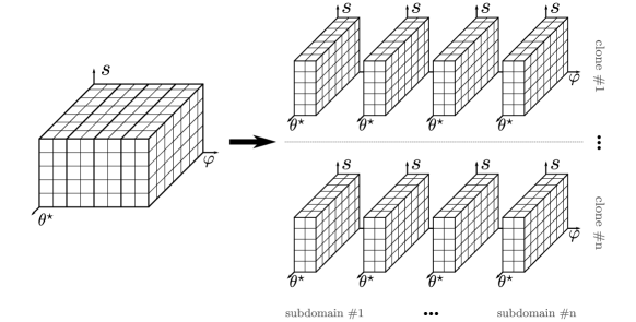
Figure 1: MPI parallelization using domain decomposition and domain cloning

The physical domain is first replicated into disjoint clones and the markers are evenly distributed among them. Each clone can be further decomposed by splitting the physical domain in the toroidal direction into subdomains. Each subdomain of each clone is attributed to an MPI task such that the total number of processes is given by $P_{\text{MPI}}=P_{\text{sub}}\times P_{\text{clones}}$, where $P_{\text{sub}}$ and $P_{\text{clones}}$ are respectively the number of tasks attributed to the subdomains and clones.

After each time step, data must be transferred between the clones and subdomains. For the clones, mainly global reductions of grid quantities are required, e.g. after each charge deposition step all the contributions from the clones must be gathered to compute the self-consistent electromagnetic fields. For the subdomains, it consists of nearest neighbour communications for the guard cells, global communications of grid data (parallel data transpose) for Fourier transforms and point to point communications of particle data where we exchange the particles that have moved from a subdomain to another. Note that in Orb5, the particle exchange algorithm is not restricted to the nearest neighbours, all-to-all is supported.

While the domain decomposition scales well with the number of subdomains, a large number of clones is problematic in terms of performance. Indeed, the domain cloning approach is quickly limited by the more demanding communications and the memory congestion due to the field data replication. To overcome this issue each MPI task is multithreaded using OpenMP. This has the main advantage of limiting the number of clones while still increasing the code performance by sharing the workload among threads.

To take advantage of the new HPC platforms equipped with accelerators, the Orb5 code has been recently ported to GPU using OpenACC. These developments will be detailed in a separate paper [78]. The choice of using OpenMP and OpenACC was motivated because they allow us to keep all options in a single source code version.

4 Results

4.1 Parallel scalability

In Fig. 2, we perform series of strong scalings of a typical electromagnetic simulation with kinetic electrons. All the runs are made on the Piz Daint supercomputer hosted at CSCS in Switzerland which is a hybrid Cray XC40/XC50 machine. For this scaling, up to 4096 compute nodes of the XC50 partition equipped with one 12-core Intel Xeon E5-2690 v3 at 2.60GHz are used.

We use as many ions as electrons, using an adaptive number of Larmor points per guiding center going from 4 to 32. The simulations are nonlinear, with a fixed number of 2 iterations for the control variate scheme. Cubic splines are used. Scalar and 1D diagnostics are computed every other time step and 2D diagnostics one step out of ten.

The starting point of each strong scaling makes a weak scaling where the grid resolution is multiplied by 2 in each dimension, the number of particles by 8 and the number of compute nodes by 8. We use domain cloning inside nodes and domain decomposition in between them, meaning that the number of clones is set to the number of cores per node, i.e. 12, and the number of subdomains to the number of nodes. We make an exception for the large-scale cases where the number of nodes exceeds the number of toroidal cells, i.e. the last points of the $640\cdot 10^{6}$ particles and $5120\cdot 10^{6}$ particles cases, in which case we double the number of clones so that the number of parallel tasks is equal to the product of subdomains and number of clones.

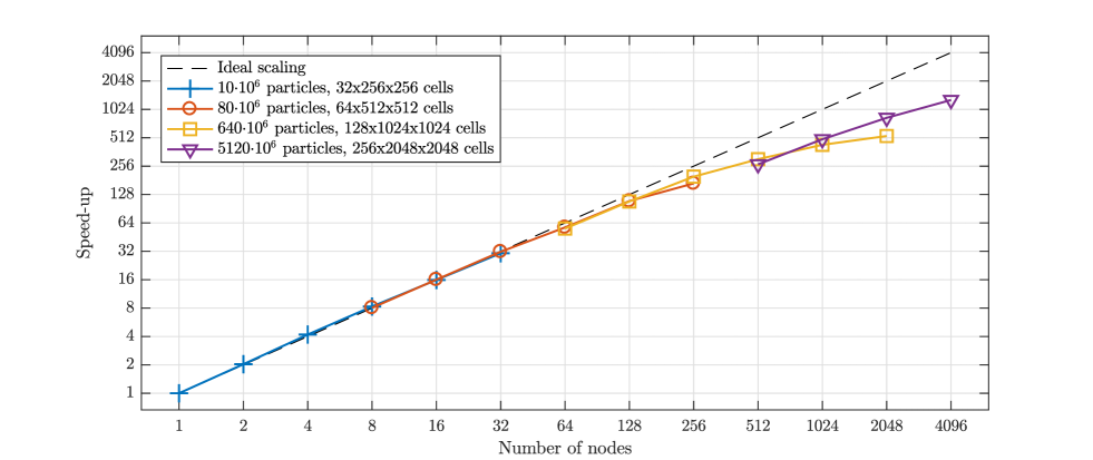
Figure 2: Strong scalings on the Piz Daint machine (Cray XC50, 12 cores per node). Speed-up is defined as inverse ratio of wall clock time to single node wall clock time, multiplied by powers of 8 for the weak scaling factor. The number of particles indicates the number of ions and the number of electrons.

Orb5 scales very well up to 128 nodes with a speed-up larger than 85% of the ideal speed-up. We even get a small superscalability from 2 to 16 nodes thanks to increased data locality and decreased memory congestion.

Above 256 nodes, the speed-up is limited mainly by the MPI communications of parallel data transpose required for the field Fourier transforms. Some effort is currently put on reducing the cost of those communications.

The performance of the GPU-accelerated Orb5 will be assessed in a following paper. In short, for scaling tests similar to Fig. 2, representative of production runs, the GPU-accelerated Orb5 is up to 4 times faster than the CPU-only code.

4.2 Strong flows and toroidal rotation

We demonstrate the use of the strong flow features of the code using an adiabatic electron CYCLONE benchmark case with nominal toroidal rotation rate $\Omega_{R}=0.2c_{s}/R$. The numerical parameters are similar to those used for typical global CYCLONE benchmark cases with sources[79] (circular concentric equilibrium, $\rho*=1/180$, $a/R=0.36$, plateau-like initial logarithmic temperature gradient profiles with $R/L_{T}=6.9$ and $R/L_{n}=2.2$). The field solver grid is $N_{s}\times N_{\theta^{\star}}\times N_{\varphi}=128\times 512\times 256$, and $1.2\times 10^{8}$ markers are used. A heating operator is used with the rate $0.013c_{s}/a$ to maintain temperature profiles near their initial value. Coarse graining is applied every $2.8a/c_{s}$ time units, with 64 bins in energy and pitch angle, and a blending factor of $1$ (so all weights in a coarse-graining bin are set equal).

The effects of strong rotation on the equilibrium have been discussed earlier for Orb5 [33], so we focus on demonstrating the operation of the code in the nonlinear regime; at the moderate levels of rotation tested here the effects are not expected to be dramatic. As in non-rotating simulations, there is some overall relaxation of the heat profiles as the turbulence driven transport commences, Figs. 3–4. The parallel flow profile, Fig 5, is not constrained by the heating operator and relaxes slightly (note that the initial parallel velocity profile is not completely flat, as might be expected for solid body rotation). In these simulations, although strong flow effects due to Centrifugal and Coriolis drift are included, the pinch driven momentum flux is expected to be nearly zero due to the use of an adiabatic electron model: this is consistent with the observation of little net momentum flux in these simulations.

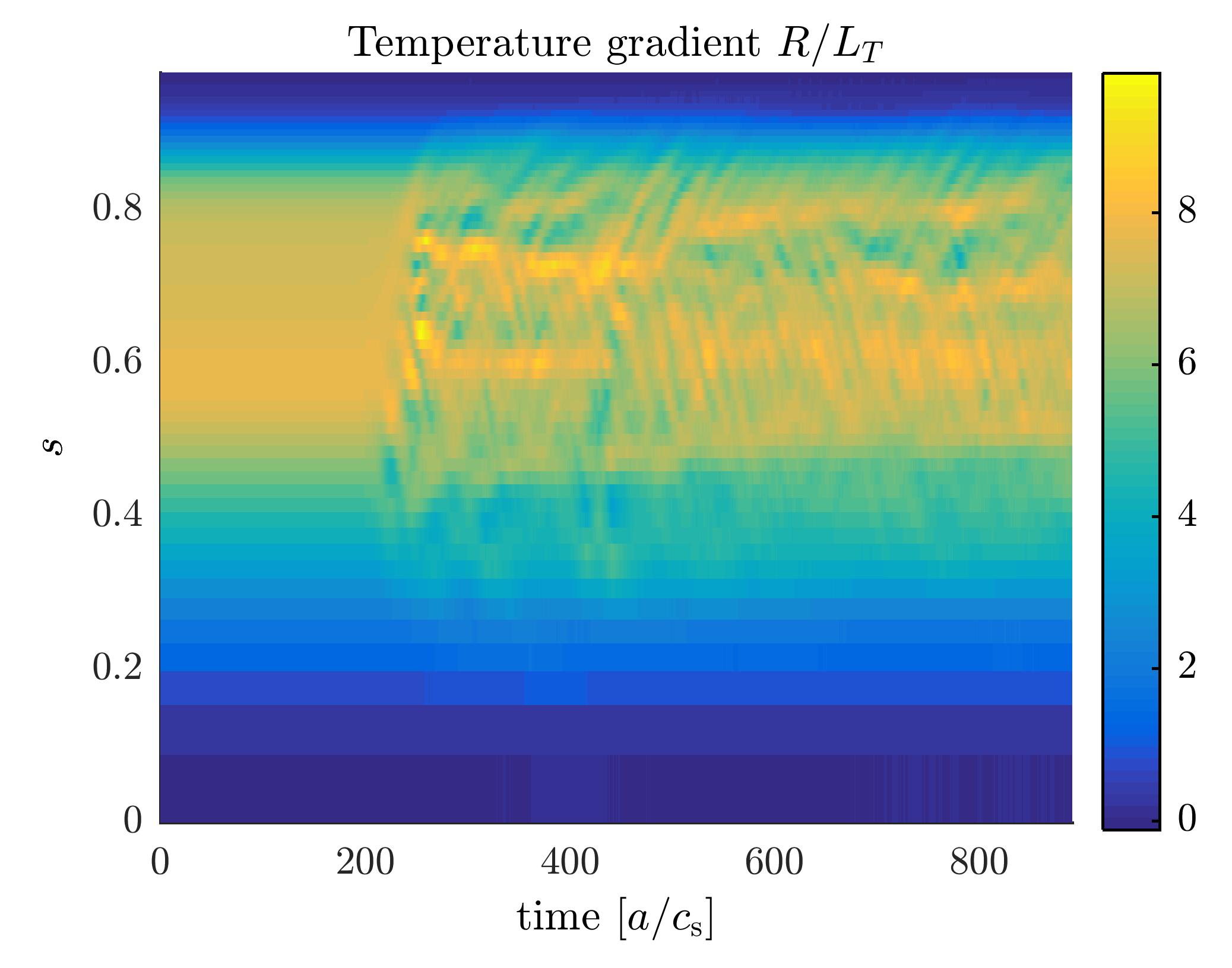
Figure 3: Temperature gradient $R/L_{T}$ versus time and radius in a strong flow simulation.

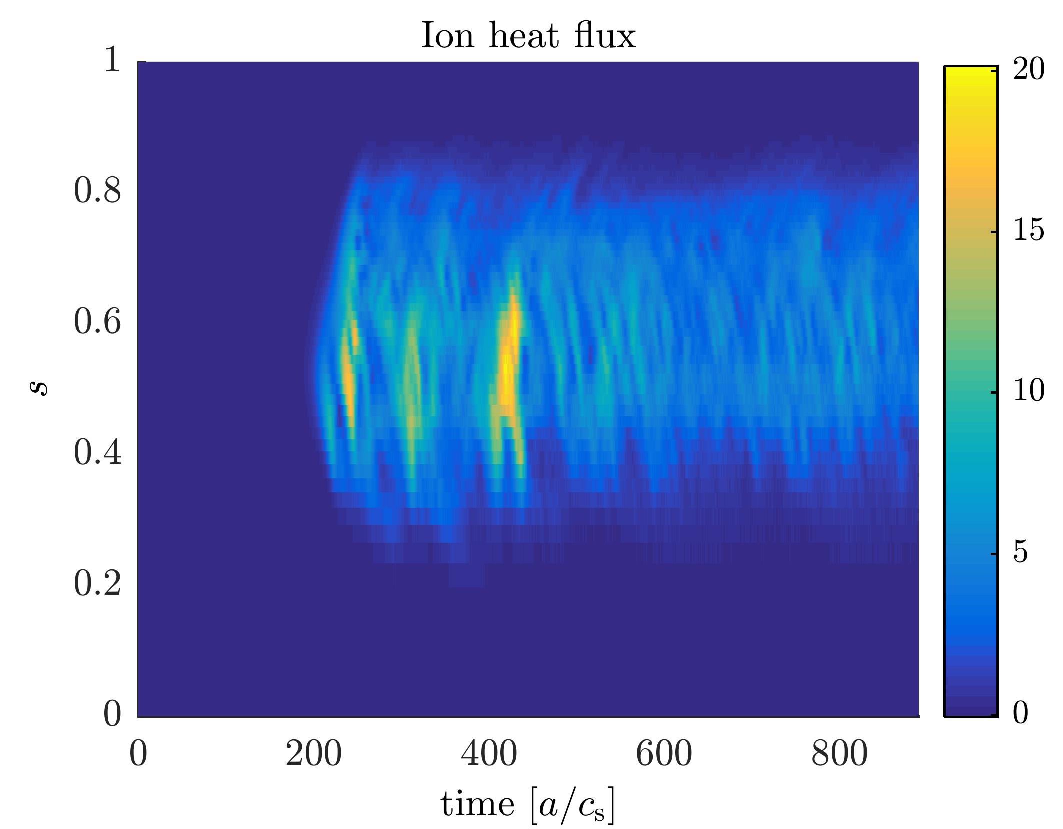
Figure 4: Ion heat flux in gyro-Bohm units versus time and radius in a strong flow simulation.

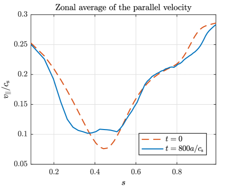
Figure 5: Zonal average of parallel velocity versus radius at the beginning (red dashed trace) and end (blue trace) of a strong flow simulation.

4.3 GK simulations of Alfvén modes in the presence of turbulence

One of the main recent developments of Orb5 has been to allow for electromagnetic simulations. The electromagnetic extension, via the control-variate scheme [68, 35] was initially implemented in 2011 [26] and proved to work for ITG instabilities. Further improvements have been necessary for having successful shear-Alfvén wave (SAW) tests, and the first results have been published in 2016 [71]. SAWs are known to be crucial in present tokamaks and future reactors, as they can be driven unstable by energetic particles (EP), which can deteriorate the EP confinement [5].

The linear dynamics of Alfvén instabilities investigated with Orb5 has been recently benchmarked against analytical theory and other codes [71, 80]. Moreover, the nonlinear dynamics of Alfvén modes due to the wave-particle nonlinearity has been investigated with Orb5, and compared with the GK code EUTERPE [81, 72], where in particular a detailed study of the saturation levels due to wave-particle nonlinearity has been carried out. Finally, after a dedicated phase of verification and benchmarking on the Alfvén dynamics, Orb5 has now started the investigation of the self-consistent interaction of Alfvén instabilities and turbulence. Here, we describe a test case where the nonlinear dynamics of an Alfvén mode is investigated in the presence of turbulence.

The tokamak geometry and magnetic field is taken consistently with Ref. [71], for the case referred to as energetic particle modes. Regarding the bulk profiles, the ion and electron temperatures are taken equal everywhere, $T_{\text{e}}(s)=T_{\text{i}}(s)$. Here, differently from Ref. [71], a value of $T_{\text{e}}(s=\text{speak})$ corresponding to $\rho^{*}=\rho_{s}/a=0.00571$, is chosen. The electron thermal to magnetic pressure ratio is $\beta_{\text{e}}=5\cdot 10^{-4}$. An analytical function is used for the profiles of the equilibrium density and temperature, for the three species of interest (thermal deuterium, labelled here as “d”, thermal electrons, labelled here as “e”, and hot deuterium, labelled here as “EP”). For the EP density, for example, the function is written as $n_{\text{EP}}(s)/n_{\text{EP}}(s_{r})=\exp\left\{-\Delta\,\kappa_{n}\tanh\left[(s-s_{r})/\Delta\right]\right\}$. The value of $\Delta$ is the same for all species, for both density and temperature: $\Delta=0.208$. Deuterium and electrons have $\kappa_{n}=0.3$ and $\kappa_{T}=1.0$, and the EP have $\kappa_{n}=10.0$ and $\kappa_{T}=0.0$. The EP temperature is given by $T_{\text{EP}}/T_{\text{e}}=100$. The distribution function of the EP population is Maxwellian in $p_{\|}$. The EP averaged concentration is $\left<n_{\text{EP}}\right>/n_{e}=0.002$. A filter allows poloidal and toroidal mode numbers with $-128<m<128$ and $0\leq n<40$ to develop. Unicity boundary conditions are imposed at s=0.0 and Dirichlet at s=1.0. A white noise initial perturbation is set at t=0. The electron mass is chosen as $m_{\text{e}}/m_{\text{i}}=0.005$. A Krook operator is applied to deuterium and electrons.

Nonlinear collisionless electromagnetic simulations have been performed with Orb5, with turbulence driven by the equilibrium temperature gradients, peaked at mid-radius with and without EP. In the absence of EP, heat transport exhibits radial corrugated structures, Fig. 6; larger corrugations are observed in the inner half of the radial domain, i.e. $s\in[0,0.5]$. Those corrugations are also present as long-lived structures in the $E\times B$ velocity profile, Fig. 7 (left), and are particularly visible for $s\in[0,0.5]$. Avalanches of $E\times B$ velocity are generated at $s\sim 0.5$ with a frequency matching the local GAM frequency, Fig. 7 (right), and then propagate outward with constant frequency. Finally, the nonzonal component of the scalar potential has been measured, and observed to grow linearly in the first so-called linear phase of the ITG turbulence, and then saturate.

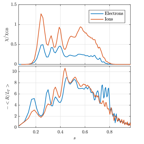
Figure 6: Corrugations of the effective heat diffusivity radial profile (top). The heat diffusivity is in gyro-Bohm units, $\chi_{\rm GB}=\rho_{\text{s}}^{2}c_{\text{s}}/a$. Radial profile of the temperature logarithmic gradient $R/L_{T}$ (bottom). All the profiles are time averaged in $t\in[500,1515]\ [a/c_{\text{s}}]$.

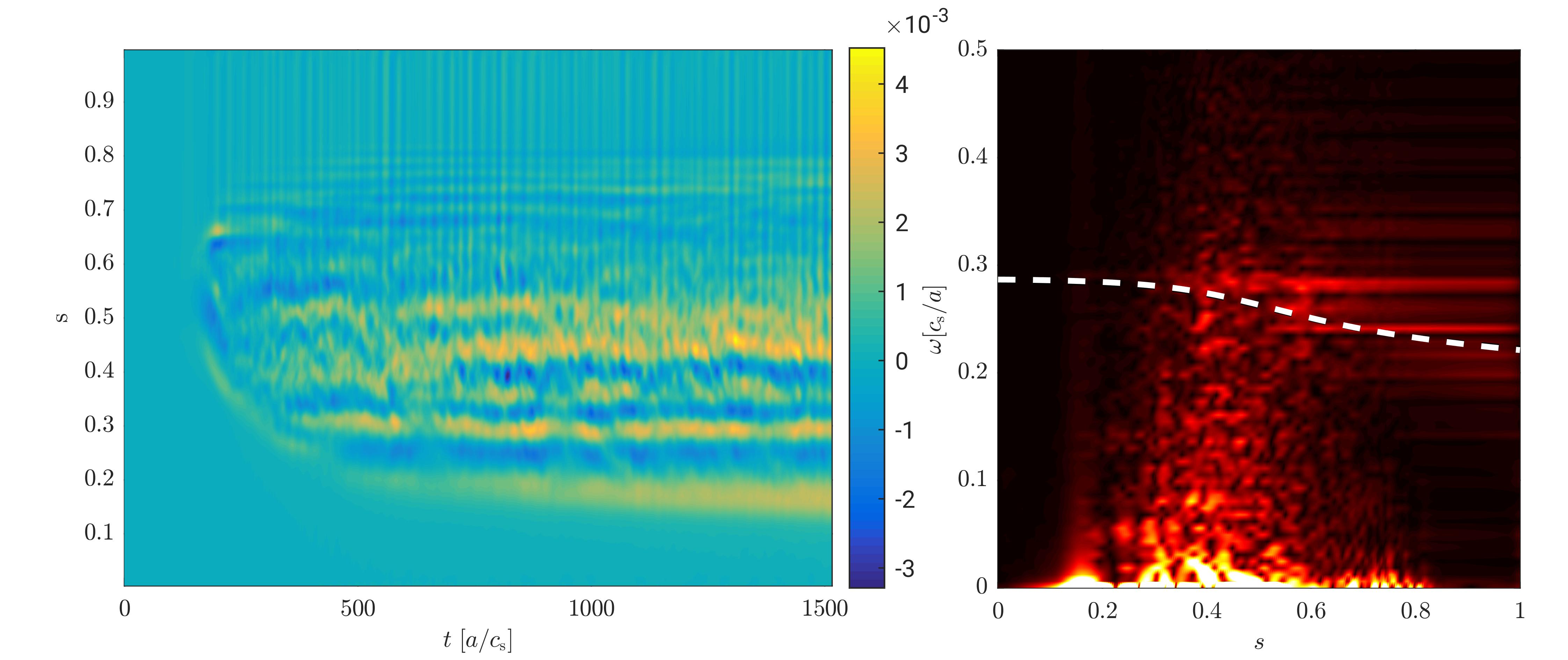
Figure 7: $E\times B$ velocity as a function of time and radius (lest) and the corresponding frequency spectrum (right). The white dashed line represents analytical estimates of the GAM frequency [82].

In the simulation where EPs are loaded, an Alfvénic instability is observed growing on top of the turbulence. Zonal structures, like zero frequency zonal flows and geodesic acoustic modes, play the role of mediators of small-scale turbulence and large-scale Alfvén modes. A comparison of the perturbed electric potential with and without EP is shown in Fig. 8.

Such simulations are numerically demanding due to the fact that they investigate intrinsically multi-scale phenomena. Thus, high resolution in space and time is needed like in turbulence simulations, the electrons must be treated kinetically for driving the current perturbations necessary for the evolution of the Alfvén physics, and three separate plasma species (thermal ions, thermal electrons, and EP) must be evolved simultaneously, in order to drive the Alfvén mode unstable, with a corresponding high number of markers adopted.

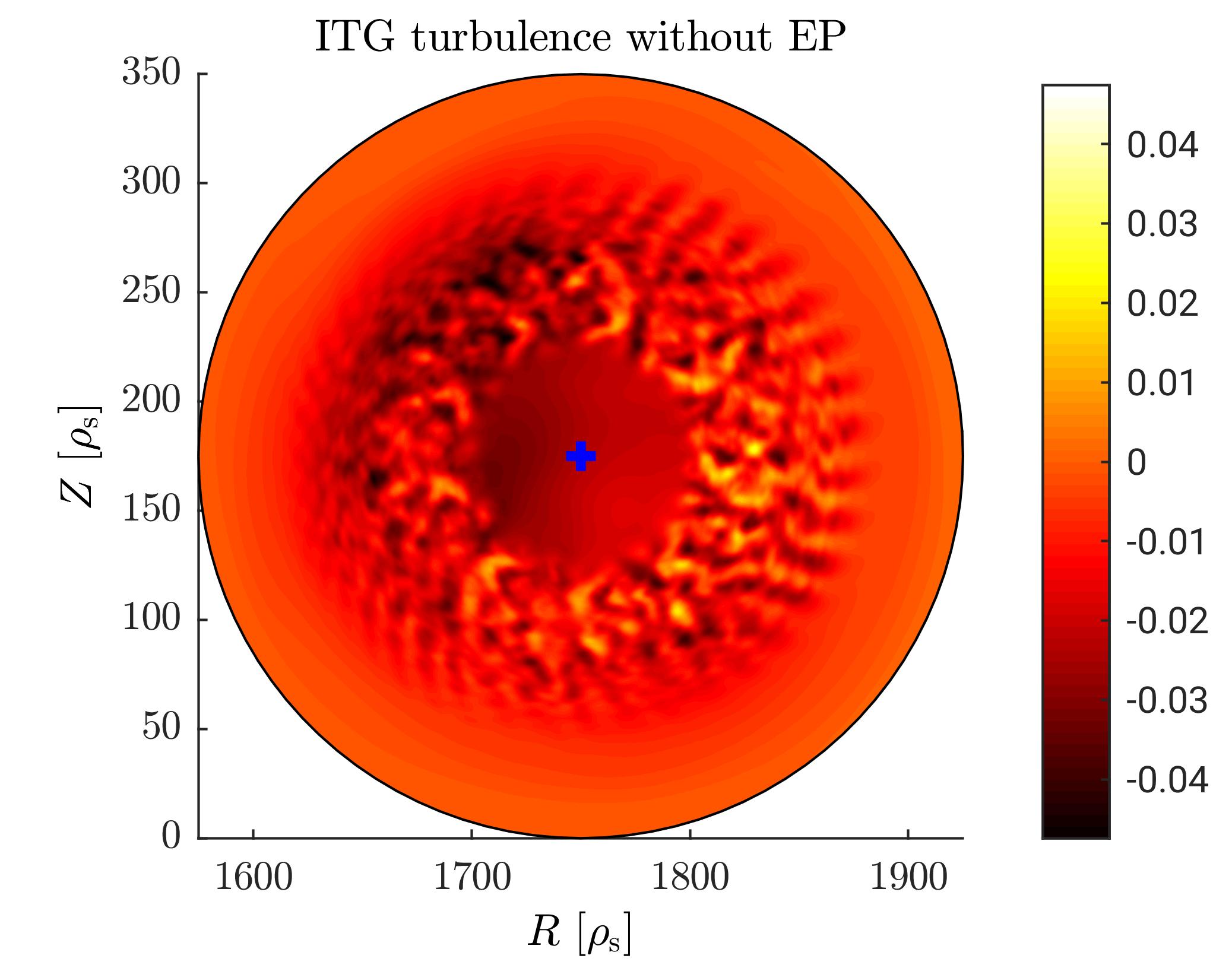
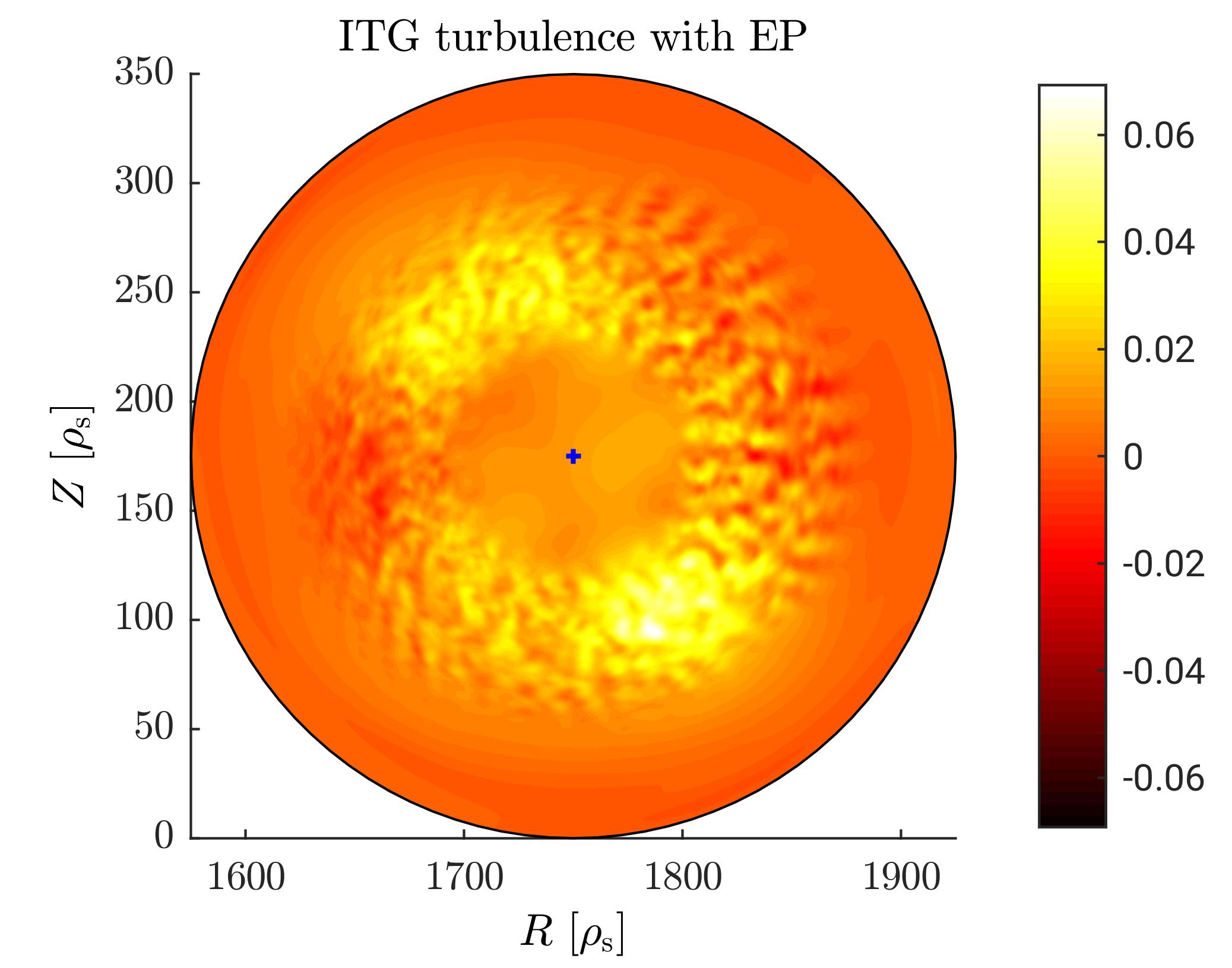
Figure 8: Poloidal cut of the perturbed potential $\phi-\overline{\phi}$. On the left, a poloidal cut showing the ITG turbulence without EP. On the right, the characteristic poloidal structure of the Alfvén instability in the presence of turbulence is shown.

5 Conclusion

Orb5 is a global PIC code used to solve the electromagnetic gyrokinetic equations in presence of collisions and various sources, e.g. heat and strong flows. The Vlasov-Maxwell model on which it relies is derived from variational principles and all the different physical approximations are included in the gyrokinetic action. This allows to consistently derive the equations of motion while ensuring conservation properties that can be later used to assess the simulation quality for example.

Three models are available for the Poisson equation in which the ion polarization density can be represented at full order, up to the second order in FLR corrections, or using a Padé approximation. On the other hand, Ampère’s equation is computed up to second order in FLR corrections. While the ions are a gyrokinetic species, the electrons can be treated as adiabatic, drift-kinetic, or an hybrid mix where passing electrons are adiabatic and trapped electrons are drift-kinetic. Furthermore, the hybrid model, which does not respect the ambipolarity condition, has been corrected.

The code is based on the PIC $\delta f$ control variate scheme in order to reduce the numerical noise due to finite particle sampling and various other techniques are used to further limit this noise, e.g. noise reduction schemes are implemented to constrain the particle weight spreading and a Fourier filter allows to solve only the physically relevant modes. The Orb5 code is parallelized using an hybrid OpenMP/MPI or OpenACC/MPI approach allowing to benefit from the many and multicore HPC systems. Scalability experiments have shown Orb5’s excellent parallel scalability up to thousands of cores.

The Orb5 code has been carefully and extensively benchmarked against various Lagrangian and Eulerian gyrokinetic codes and always showed a good agreement in the results [79, 83, 84, 85, 80, 86]. A few physical simulations run with the Orb5 code and including e.g. strong flows, toroidal rotation, and shear Alfvén waves are also presented to illustrate the capabilities of the code.

6 Acknowledgments

The authors deeply acknowledge past valuable contributions of Dr. T. M. Tran to the Orb5 code development. Fruitful discussions with S. Ethier are gratefully acknowledged.

The authors thank the CSCS for providing access to the full Piz Daint machine to perform the scalability tests. This work was supported by a grant from the Swiss National Supercomputing Centre (CSCS) under project ID s760. This work has been carried out within the framework of the EUROfusion Consortium and has received funding from the Euratom research and training programme 2014-2018 and 2019-2020 under grant agreement No 633053. The views and opinions expressed herein do not necessarily reflect those of the European Commission. This work was partly supported by the Swiss National Science Foundation.

References

References

-
[1]
R. J. Fonck, G. Cosby, R. D. Durst, S. F. Paul, N. Bretz, S. Scott,
E. Synakowski, G. Taylor,
Long-wavelength
density turbulence in the TFTR tokamak, Phys. Rev. Lett. 70 (24) (1993)
3736–3739.
doi:10.1103/PhysRevLett.70.3736.
URL https://link.aps.org/doi/10.1103/PhysRevLett.70.3736 -
[2]
S. J. Zweben, J. A. Boedo, O. Grulke, C. Hidalgo, B. LaBombard, R. J. Maqueda,
P. Scarin, J. L. Terry,
Edge
turbulence measurements in toroidal fusion devices, Plasma Phys. Control.
Fusion 49 (7) (2007) S1–S23.
doi:10.1088/0741-3335/49/7/S01.
URL http://stacks.iop.org/0741-3335/49/i=7/a=S01?key=crossref.b88a2f06af2f78dc5d83138198588e28 -
[3]
W. Horton, Drift waves and
transport, Rev. Mod. Phys. 71 (3) (1999) 735–778.
doi:10.1103/RevModPhys.71.735.
URL http://link.aps.org/doi/10.1103/RevModPhys.71.735https://link.aps.org/doi/10.1103/RevModPhys.71.735 -
[4]
C. Cheng, L. Chen, M. Chance,
High-n
ideal and resistive shear Alfvén waves in tokamaks, Ann. Phys. (N.
Y). 161 (1) (1985) 21–47.
doi:10.1016/0003-4916(85)90335-5.
URL https://www.sciencedirect.com/science/article/pii/0003491685903355?via{%}3Dihub -
[5]
L. Chen, F. Zonca,
Physics of
Alfvén waves and energetic particles in burning plasmas, Rev. Mod.
Phys. 88 (1) (2016) 015008.
doi:10.1103/RevModPhys.88.015008.
URL https://link.aps.org/doi/10.1103/RevModPhys.88.015008 -
[6]
A. J. Brizard, T. Hahm, Foundations
of nonlinear gyrokinetic theory, Rev. Mod. Phys. 79 (2) (2007) 421–468.
doi:10.1103/RevModPhys.79.421.
URL http://link.aps.org/doi/10.1103/RevModPhys.79.421http://journals.aps.org/rmp/abstract/10.1103/RevModPhys.79.421 -
[7]
N. Tronko, C. Chandre,
Second order nonlinear gyrokinetic theory :
From the particle to the gyrocenter, J. Plasma Phys. 84 (3).
arXiv:1709.05222,
doi:10.1017/s0022377818000430.
URL https://www.cambridge.org/core/journals/journal-of-plasma-physics/article/secondorder-nonlinear-gyrokinetic-theory-from-the-particle-to-the-gyrocentre/C377BD7B6F0E11D8EB6E3D92AD97C7FEhttp://arxiv.org/abs/1709.05222 -
[8]
X. Garbet, Y. Idomura, L. Villard, T. H. Watanabe,
Gyrokinetic
simulations of turbulent transport (apr 2010).
doi:10.1088/0029-5515/50/4/043002.
URL http://stacks.iop.org/0029-5515/50/i=4/a=043002?key=crossref.c0e169b0cfa8ae95a37226a468dc019b -
[9]
S. Jolliet, A. Bottino, P. Angelino, R. Hatzky, T. Tran, B. F. B. Mcmillan,
O. Sauter, K. Appert, Y. Idomura, L. Villard,
A global
collisionless PIC code in magnetic coordinates, Comput. Phys. Commun.
177 (5) (2007) 409–425.
doi:10.1016/j.cpc.2007.04.006.
URL http://linkinghub.elsevier.com/retrieve/pii/S0010465507002251http://www.sciencedirect.com/science/article/pii/S0010465507002251 -
[10]
Y. Idomura, S. Tokuda, Y. Kishimoto,
Global
gyrokinetic simulation of ion temperature gradient driven turbulence in
plasmas using a canonical Maxwellian distribution, Nucl. Fusion 43 (4)
(2003) 234–243.
doi:10.1088/0029-5515/43/4/303.
URL http://iopscience.iop.org/article/10.1088/0029-5515/43/4/303http://stacks.iop.org/0029-5515/43/i=4/a=303?key=crossref.d169703164fcc8d437dddf6f6a74be33 -
[11]
Z. Lin, T. S. Hahm, W. W. Lee, W. M. Tang, R. B. White,
Turbulent transport
reduction by zonal flows: Massively parallel simulations, Science (80-. ).
281 (5384) (1998) 1835–1837.
doi:10.1126/science.281.5384.1835.
URL http://www.ncbi.nlm.nih.gov/pubmed/9743492 -
[12]
S. Ku, C. S. Chang, R. Hager, R. M. Churchill, G. R. Tynan, I. Cziegler,
M. Greenwald, J. Hughes, S. E. Parker, M. F. Adams, E. D’Azevedo, P. Worley,
A fast low-to-high
confinement mode bifurcation dynamics in the boundary-plasma gyrokinetic code
XGC1, Phys. Plasmas 25 (5) (2018) 056107.
doi:10.1063/1.5020792.
URL http://aip.scitation.org/doi/10.1063/1.5020792 -
[13]
W. X. Wang, T. S. Hahm, W. W. Lee, G. Rewoldt, J. Manickam, W. M. Tang,
Nonlocal properties of
gyrokinetic turbulence and the role of ExB flow shear, Phys. Plasmas 14 (7)
(2007) 072306.
doi:10.1063/1.2750647.
URL http://aip.scitation.org/doi/10.1063/1.2750647 -
[14]
A. M. Dimits, T. J. Williams, J. A. Byers, B. I. Cohen,
Scalings of
ion-temperature-gradient-driven anomalous transport in tokamaks, Phys. Rev.
Lett. 77 (1) (1996) 71–74.
doi:10.1103/PhysRevLett.77.71.
URL https://link.aps.org/doi/10.1103/PhysRevLett.77.71 -
[15]
T. Korpilo, A. Gurchenko, E. Gusakov, J. Heikkinen, S. Janhunen, T. Kiviniemi,
S. Leerink, P. Niskala, A. Perevalov,
Gyrokinetic
full-torus simulations of ohmic tokamak plasmas in circular limiter
configuration, Comput. Phys. Commun. 203 (2016) 128–137.
doi:10.1016/J.CPC.2016.02.021.
URL https://www.sciencedirect.com/science/article/pii/S0010465516300364?via{%}3Dihub -
[16]
F. Jenko, W. Dorland, M. Kotschenreuther, B. N. Rogers,
Electron temperature
gradient driven turbulence, Phys. Plasmas 7 (5) (2000) 1904.
doi:10.1063/1.874014.
URL https://aip.scitation.org/doi/10.1063/1.874014 -
[17]
Y. Idomura, M. Ida, T. Kano, N. Aiba, S. Tokuda,
Conservative
global gyrokinetic toroidal full-f five-dimensional Vlasov simulation,
Comput. Phys. Commun. 179 (6) (2008) 391–403.
doi:10.1016/j.cpc.2008.04.005.
URL https://www.sciencedirect.com/science/article/pii/S0010465508001409?via{%}3Dihub -
[18]
J. Candy, R. E. Waltz,
An
Eulerian gyrokinetic-Maxwell solver, J. Comput. Phys. 186 (2) (2003)
545–581.
doi:10.1016/S0021-9991(03)00079-2.
URL https://www.sciencedirect.com/science/article/pii/S0021999103000792https://www.sciencedirect.com/science/article/pii/S0021999103000792?via{%}3Dihub -
[19]
A. G. Peeters, D. Strintzi,
The effect of a
uniform radial electric field on the toroidal ion temperature gradient
mode, Phys. Plasmas 11 (8) (2004) 3748–3751.
doi:10.1063/1.1762876.
URL http://aip.scitation.org/doi/10.1063/1.1762876 -
[20]
T.-H. H. Watanabe, H. Sugama,
Velocity–space
structures of distribution function in toroidal ion temperature gradient
turbulence, Nucl. Fusion 46 (1) (2006) 24–32.
doi:10.1088/0029-5515/46/1/003.
URL http://stacks.iop.org/0029-5515/46/i=1/a=003?key=crossref.3d7e6f40ce52b566eca20514f822347d -
[21]
M. Kotschenreuther, G. Rewoldt, W. M. Tang,
Comparison
of initial value and eigenvalue codes for kinetic toroidal plasma
instabilities, Comput. Phys. Commun. 88 (2-3) (1995) 128–140.
doi:10.1016/0010-4655(95)00035-E.
URL https://www.sciencedirect.com/science/article/pii/001046559500035E?via{%}3Dihub -
[22]
V. Grandgirard, J. Abiteboul, J. Bigot, T. Cartier-Michaud, N. Crouseilles,
G. Dif-Pradalier, C. Ehrlacher, D. Esteve, X. Garbet, P. Ghendrih, G. Latu,
M. Mehrenberger, C. Norscini, C. Passeron, F. Rozar, Y. Sarazin,
E. Sonnendrücker, A. Strugarek, D. Zarzoso,
A 5D
gyrokinetic full-f global semi-Lagrangian code for flux-driven ion turbulence
simulations, Comput. Phys. Commun. 207 (2016) 35–68.
doi:10.1016/j.cpc.2016.05.007.
URL http://linkinghub.elsevier.com/retrieve/pii/S0010465516301230 - [23] C. K. Birdsall, A. B. Langdon, Plasma Physics via Computer simulations, CRC press, 2004.
-
[24]
W. W. Lee,
Gyrokinetic particle
simulation model, J. Comput. Phys. 72 (1) (1987) 243–269.
doi:10.1016/0021-9991(87)90080-5.
URL http://www.sciencedirect.com/science/article/pii/0021999187900805https://aip.scitation.org/doi/10.1063/1.864140 - [25] T. M. Tran, K. Appert, M. Fivaz, G. Jost, J. Vaclavik, L. Villard, Global gyrokinetic simulation of ion-temperature-gradient-driven instabilities using particles, in: Theory of fusion plasmas, Societa Italiana di Fisica, 1999, p. 45.
-
[26]
A. Bottino, T. Vernay, B. Scott, S. Brunner, R. Hatzky, S. Jolliet, B. F.
McMillan, T. M. Tran, L. Villard,
Global
simulations of tokamak microturbulence: Finite- effects and
collisions, Plasma Phys. Control. Fusion 53 (12) (2011) 124027.
doi:10.1088/0741-3335/53/12/124027.
URL http://stacks.iop.org/0741-3335/53/i=12/a=124027?key=crossref.7fb008935b961f69d91dc474edce4036 -
[27]
T. Vernay, S. Brunner, L. Villard, B. F. McMillan, S. Jolliet, T. M. Tran,
A. Bottino, J. P. Graves,
Neoclassical equilibria as
starting point for global gyrokinetic microturbulence simulations, Phys.
Plasmas 17 (12) (2010) 122301.
doi:10.1063/1.3519513.
URL http://pop.aip.org/resource/1/phpaen/v17/i12/p122301{_}s1http://aip.scitation.org/doi/10.1063/1.3519513 -
[28]
S. Jolliet, Gyrokinetic
particle-in-cell global simulations of ion-temperature-gradient and
collisionless-trapped-electron-mode turbulence in tokamaks, Ph.D. thesis,
École Polytechnique Fédérale de Lausanne (2009).
doi:10.5075/epfl-thesis-4326.
URL https://infoscience.epfl.ch/record/130837?ln=fr -
[29]
T. Vernay, S. Brunner, L. Villard, B. F. McMillan, S. Jolliet, A. Bottino,
T. Görler, F. Jenko,
Global
gyrokinetic simulations of TEM microturbulence, Plasma Phys. Control.
Fusion 55 (7) (2013) 074016.
doi:10.1088/0741-3335/55/7/074016.
URL http://stacks.iop.org/0741-3335/55/i=7/a=074016?key=crossref.6e26708d569dcb2dcd6631cc3a584de7 -
[30]
J. Dominski, B. F. McMillan, S. Brunner, G. Merlo, T. M. Tran, L. Villard,
An arbitrary wavelength solver for
global gyrokinetic simulations. Application to the study of fine radial
structures on microturbulence due to non-adiabatic passing electron
dynamics, Phys. Plasmas 24 (2).
doi:10.1063/1.4976120.
URL http://dx.doi.org/10.1063/1.4976120http://aip.scitation.org/toc/php/24/2 -
[31]
B. F. McMillan, S. Jolliet, T. M. Tran, L. Villard, A. Bottino, P. Angelino,
Long global
gyrokinetic simulations: Source terms and particle noise control, Phys.
Plasmas 15 (5) (2008) 1–10.
doi:10.1063/1.2921792.
URL http://aip.scitation.org/doi/10.1063/1.2921792 -
[32]
S. Jolliet, B. F. McMillan, T. Vernay, L. Villard, A. Bottino, P. Angelino,
Quasisteady and steady
states in global gyrokinetic particle-in-cell simulations, Phys Plasmas
16 (5) (2009) 52307–52310.
doi:10.1063/1.3140036.
URL http://link.aip.org/link/?PHP/16/052307/1 -
[33]
J. D. Collier, B. F. McMillan, J. R. Robinson,
Global gyrokinetic
simulations with strong flows, Phys. Plasmas 23 (11) (2016) 112503.
doi:10.1063/1.4965900.
URL http://aip.scitation.org/doi/10.1063/1.4965900 -
[34]
A. Mishchenko, A. Bottino, R. Hatzky, E. Sonnendrücker, R. Kleiber,
A. Könies,
Mitigation of the
cancellation problem in the gyrokinetic particle-in-cell simulations of
global electromagnetic modes, Phys. Plasmas 24 (8) (2017) 081206.
doi:10.1063/1.4997540.
URL http://aip.scitation.org/doi/10.1063/1.4997540 -
[35]
R. Hatzky, A. Könies, A. Mishchenko,
Electromagnetic
gyrokinetic PIC simulation with an adjustable control variates method, J.
Comput. Phys. 225 (1) (2007) 568–590.
doi:10.1016/j.jcp.2006.12.019.
URL https://www.sciencedirect.com/science/article/pii/S0021999106006085 -
[36]
R. Hatzky, R. Kleiber, A. Könies, A. Mishchenko, M. Borchardt,
A. Bottino, E. Sonnendrücker,
Reduction
of the statistical error in electromagnetic gyrokinetic particle-in-cell
simulations, J. Plasma Phys. 85 (1) (2019) 905850112.
doi:10.1017/S0022377819000096.
URL https://www.cambridge.org/core/product/identifier/S0022377819000096/type/journal{_}article -
[37]
A. Mishchenko, A. Bottino, A. Biancalani, R. Hatzky, T. Hayward-Schneider,
N. Ohana, E. Lanti, S. Brunner, L. Villard, M. Borchardt, R. Kleiber,
A. Koenies,
Pullback scheme implementation in ORB5,
Comput. Phys. Commun.arXiv:1811.05346, doi:arXiv:1811.05346v1.
URL https://www.sciencedirect.com/science/article/pii/S0010465518304181?dgcid=rss{_}sd{_}allhttp://arxiv.org/abs/1811.05346 -
[38]
T. Vernay, S. Brunner, L. Villard, B. F. McMillan, S. Jolliet, T. M. Tran,
A. Bottino,
Synergy
between ion temperature gradient turbulence and neoclassical processes in
global gyrokinetic particle-in-cell simulations, Phys. Plasmas 19 (4)
(2012) 042301.
doi:10.1063/1.3699189.
URL http://scitation.aip.org/content/aip/journal/pop/19/4/10.1063/1.3699189 -
[39]
E. Sonnendrücker, A. Wacher, R. Hatzky, R. Kleiber,
A
split control variate scheme for PIC simulations with collisions, J.
Comput. Phys. 295 (2015) 402–419.
doi:10.1016/j.jcp.2015.04.004.
URL https://www.sciencedirect.com/science/article/pii/S0021999115002442?via{%}3Dihub -
[40]
H. Lütjens, A. Bondeson, O. Sauter,
The
CHEASE code for toroidal MHD equilibria, Comput. Phys. Commun. 97 (3)
(1996) 219–260.
doi:10.1016/0010-4655(96)00046-X.
URL https://www.sciencedirect.com/science/article/pii/001046559600046X -
[41]
H. Sugama, Gyrokinetic field theory,
Phys. Plasmas 7 (2) (2000) 466–480.
doi:10.1063/1.873832.
URL http://aip.scitation.org/doi/abs/10.1063/1.873832http://aip.scitation.org/doi/10.1063/1.873832 -
[42]
N. Tronko, A. Bottino, E. Sonnendrücker,
Second order
gyrokinetic theory for particle-in-cell codes, Phys. Plasmas 23 (8) (2016)
082505.
arXiv:1604.03538,
doi:10.1063/1.4960039.
URL http://aip.scitation.org/doi/10.1063/1.4960039 -
[43]
N. Tronko, A. Bottino, C. Chandre, E. Sonnendruecker,
Hierarchy
of second order gyrokinetic Hamiltonian models for particle-in-cell codes,
Plasma Phys. Control. Fusion 59 (6) (2017) 064008.
arXiv:1703.05095,
doi:10.1088/1361-6587/aa68af.
URL http://stacks.iop.org/0741-3335/59/i=6/a=064008?key=crossref.0311bba6987f428be09915498fafb4f3 -
[44]
E. Lanti, J. Dominski, S. Brunner, B. F. McMillan, L. Villard,
Padé
approximation of the adiabatic electron contribution to the gyrokinetic
quasi-neutrality equation in the ORB5 code, J. Phys. Conf. Ser. 775 (1)
(2016) 012006.
doi:10.1088/1742-6596/775/1/012006.
URL http://stacks.iop.org/1742-6596/775/i=1/a=012006?key=crossref.5970237ead440732086f3dc78b4903bc -
[45]
Y. Idomura, A new hybrid
kinetic electron model for full-f gyrokinetic simulations, J. Comput. Phys.
313 (2016) 511–531.
doi:10.1016/j.jcp.2016.02.057.
URL http://dx.doi.org/10.1016/j.jcp.2016.02.057 -
[46]
A. Y. Aydemir,
A
unified Monte Carlo interpretation of particle simulations and applications
to non-neutral plasmas, Phys. Plasmas 1 (4) (1994) 822.
doi:10.1063/1.870740.
URL http://scitation.aip.org/content/aip/journal/pop/1/4/10.1063/1.870740 -
[47]
P. Angelino, A. Bottino, R. Hatzky, S. Jolliet, O. Sauter, T. M. Tran,
L. Villard, On
the definition of a kinetic equilibrium in global gyrokinetic simulations,
Phys. Plasmas 13 (5) (2006) 052304.
doi:10.1063/1.2193947.
URL http://aip.scitation.org/doi/10.1063/1.2193947http://scitation.aip.org/content/aip/journal/pop/13/5/10.1063/1.2193947 -
[48]
T. S. Hahm, Nonlinear gyrokinetic
equations for turbulence in core transport barriers, Phys. Plasmas 3 (12)
(1996) 4658–4664.
doi:10.1063/1.872034.
URL https://aip.scitation.org/doi/10.1063/1.872034http://aip.scitation.org/doi/10.1063/1.872034 -
[49]
L. Guazzotto, R. Betti, J. Manickam, S. Kaye,
Numerical study of
tokamak equilibria with arbitrary flow, Phys. Plasmas 11 (2) (2004)
604–614.
doi:10.1063/1.1637918.
URL http://aip.scitation.org/doi/10.1063/1.1637918 -
[50]
G. Dif-Pradalier, V. Grandgirard, Y. Sarazin, X. Garbet, P. Ghendrih,
Interplay
between gyrokinetic turbulence, flows, and collisions: Perspectives on
transport and poloidal rotation, Phys. Rev. Lett. 103 (6) (2009) 065002.
doi:10.1103/PhysRevLett.103.065002.
URL https://link.aps.org/doi/10.1103/PhysRevLett.103.065002 -
[51]
Z. Lin, W. M. Tang, W. W. Lee,
Gyrokinetic particle
simulation of neoclassical transport, Phys. Plasmas 2 (8) (1995)
2975–2988.
doi:10.1063/1.871196.
URL http://aip.scitation.org/doi/10.1063/1.871196 -
[52]
S. Brunner, E. Valeo, J. A. Krommes,
Collisional
delta-f scheme with evolving background for transport time scale
simulations, Phys. Plasmas 6 (12) (1999) 4504–4521.
doi:doi:10.1063/1.873738.
URL http://pop.aip.org/resource/1/phpaen/v6/i12/p4504{_}s1{%}5Cnhttp://scitation.aip.org/getpdf/servlet/GetPDFServlet?filetype=pdf{&}id=PHPAEN000006000012004504000001{&}idtype=cvips{&}doi=10.1063/1.873738{&}prog=normal -
[53]
S. E. Parker, W. W. Lee,
A fully nonlinear
characteristic method for gyrokinetic simulation, Phys. Fluids B 5 (1)
(1993) 77–86.
doi:10.1063/1.860870.
URL http://aip.scitation.org/doi/10.1063/1.860870 -
[54]
G. Hu, J. A. Krommes,
Generalized weighting
scheme for f particle simulation method, Phys. Plasmas 1 (4)
(1994) 863–874.
doi:10.1063/1.870745.
URL http://aip.scitation.org/doi/10.1063/1.870745 -
[55]
S. J. Allfrey, R. Hatzky,
A
revised f algorithm for nonlinear PIC simulation, Comput. Phys.
Commun. 154 (2) (2003) 98–104.
doi:10.1016/S0010-4655(03)00288-1.
URL https://www.sciencedirect.com/science/article/pii/S0010465503002881?via{%}3Dihub -
[56]
J. H. Halton, On the
efficiency of certain quasi-random sequences of points in evaluating
multi-dimensional integrals, Numer. Math. 2 (1) (1960) 84–90.
doi:10.1007/BF01386213.
URL http://link.springer.com/10.1007/BF01386213 -
[57]
J. M. Hammersley,
Monte carlo
methods for solving multivariable problems, Ann. N. Y. Acad. Sci. 86 (3)
(1960) 844–874.
doi:10.1111/j.1749-6632.1960.tb42846.x.
URL http://doi.wiley.com/10.1111/j.1749-6632.1960.tb42846.x - [58] J. G. van der Corput, Verteilungsfunktionen. I. Mitt., Proc. Akad. Wet. Amsterdam 38 (1935) 813–821.
-
[59]
B. McMillan, S. Jolliet, A. Bottino, P. Angelino, T. Tran, L. Villard,
Rapid
Fourier space solution of linear partial integro-differential equations in
toroidal magnetic confinement geometries, Comput. Phys. Commun. 181 (4)
(2010) 715–719.
doi:10.1016/j.cpc.2009.12.001.
URL http://linkinghub.elsevier.com/retrieve/pii/S0010465509003920http://www.sciencedirect.com/science/article/pii/S0010465509003920 -
[60]
M. Frigo, S. G. Johnson,
The design and
implementation of FFTW3, in: Proc. IEEE, Vol. 93, 2005, pp. 216–231.
doi:10.1109/JPROC.2004.840301.
URL http://ieeexplore.ieee.org/document/1386650/ -
[61]
E. Anderson, Z. Bai, C. Bischof, L. S. Blackford, J. Demmel, J. Dongarra,
J. Du Croz, A. Greenbaum, S. Hammarling, A. McKenney, D. Sorensen,
LAPACK Users’
Guide, Society for Industrial and Applied Mathematics, 1999.
doi:10.1137/1.9780898719604.
URL http://epubs.siam.org/doi/book/10.1137/1.9780898719604 -
[62]
R. Hatzky, T. M. Tran, A. Könies, R. Kleiber, S. J. Allfrey,
Energy conservation in
a nonlinear gyrokinetic particle-in-cell code for
ion-temperature-gradient-driven modes in -pinch geometry, Phys.
Plasmas 9 (3) (2002) 898.
doi:10.1063/1.1449889.
URL http://aip.scitation.org/doi/10.1063/1.1449889 -
[63]
Y. Chen, S. E. Parker,
Coarse-graining phase
space in f particle-in-cell simulations, Phys. Plasmas 14 (8)
(2007) 082301.
doi:10.1063/1.2751603.
URL http://aip.scitation.org/doi/10.1063/1.2751603 -
[64]
W. Dorland, Gyrokinetic
Turbulence Simulations (may 2001).
doi:10.1063/1.1351828.
URL http://aip.scitation.org/doi/10.1063/1.1351828 -
[65]
Y. Chen, S. E. Parker,
A
f particle method for gyrokinetic simulations with kinetic electrons
and electromagnetic perturbations, J. Comput. Phys. 189 (2) (2003)
463–475.
doi:10.1016/S0021-9991(03)00228-6.
URL https://www.sciencedirect.com/science/article/pii/S0021999103002286 -
[66]
A. Mishchenko, R. Hatzky, A. Könies,
Conventional
f-particle simulations of electromagnetic perturbations with finite
elements, Phys. Plasmas 11 (12) (2004) 5480–5486.
doi:10.1063/1.1812275.
URL http://aip.scitation.org/doi/10.1063/1.1812275 - [67] A. Mishchenko, A. Könies, R. Hatzky, Gyrokinetic simulations with a particle discretization of the field equations, in: Proc. Jt. Varenna-Lausanne Int. Work., Societa Italiana di Fisica, Bologna, 2004, p. 315.
-
[68]
A. Mishchenko, A. Könies, R. Kleiber, M. Cole,
Pullback
transformation in gyrokinetic electromagnetic simulations, Phys. Plasmas
21 (9) (2014) 092110.
arXiv:1407.3992,
doi:10.1063/1.4895501.
URL http://aip.scitation.org/doi/10.1063/1.4895501 -
[69]
R. Kleiber, R. Hatzky, A. Könies, A. Mishchenko, E. Sonnendrücker,
An explicit large time
step particle-in-cell scheme for nonlinear gyrokinetic simulations in the
electromagnetic regime, Phys. Plasmas 23 (3) (2016) 032501.
doi:10.1063/1.4942788.
URL http://aip.scitation.org/doi/10.1063/1.4942788 -
[70]
A. Mishchenko, M. Cole, R. Kleiber, A. Könies,
New variables for
gyrokinetic electromagnetic simulations, Phys. Plasmas 21 (5) (2014)
052113.
doi:10.1063/1.4880560.
URL http://aip.scitation.org/doi/10.1063/1.4880560 -
[71]
A. Biancalani, A. Bottino, S. Briguglio, A. Könies, P. Lauber,
A. Mishchenko, E. Poli, B. D. Scott, F. Zonca,
Linear gyrokinetic
particle-in-cell simulations of Alfvén instabilities in tokamaks,
Phys. Plasmas 23 (1) (2016) 012108.
arXiv:1510.01945,
doi:10.1063/1.4939803.
URL http://aip.scitation.org/doi/10.1063/1.4939803 -
[72]
A. Biancalani, A. Bottino, M. Cole, C. Di Troia, P. Lauber, A. Mishchenko,
B. Scott, F. Zonca,