Transferable Knowledge for Low-cost Decision Making in Cloud Environments

Abstract

Users of cloud computing are increasingly overwhelmed with the wide range of providers and services offered by each provider. As such, many users select cloud services based on description alone. An emerging alternative is to use a decision support system (DSS), which typically relies on gaining insights from observational data in order to assist a customer in making decisions regarding optimal deployment or redeployment of cloud applications. The primary activity of such systems is the generation of a prediction model (e.g. using machine learning), which requires a significantly large amount of training data. However, considering the varying architectures of applications, cloud providers, and cloud offerings, this activity is not sustainable as it incurs additional time and cost to collect training data and subsequently train the models. We overcome this through developing a Transfer Learning (TL) approach where the knowledge (in the form of the prediction model and associated data set) gained from running an application on a particular cloud infrastructure is transferred in order to substantially reduce the overhead of building new models for the performance of new applications and/or cloud infrastructures. In this paper, we present our approach and evaluate it through extensive experimentation involving three real world applications over two major public cloud providers, namely Amazon and Google. Our evaluation shows that our novel two-mode TL scheme increases overall efficiency with a factor of 60% reduction in the time and cost of generating a new prediction model. We test this under a number of cross-application and cross-cloud scenarios.

1.   Introduction

The cloud computing market has a proliferation of service offerings, pricing models, and technology standards [33, 14]. This complicates decisions making regarding service selection [35, 26]. Although such challenges apply to all levels of cloud services, the Infrastructure as a Service (IaaS) level is particularly difficult given the fact that IaaS provides more choices and control for developers. In the IaaS domain, there is a wide range of virtual machines (VM) on offer – see Figure 1 – but no straightforward method to compare their performance and, more generally, cost/performance trade-offs, neither within nor across cloud providers. A wrong or suboptimal decision can result in financial loss as well as reduced application performance [35, 41, Ghrada2018cloudvnf], a common concern of end users [11, 27, 2].

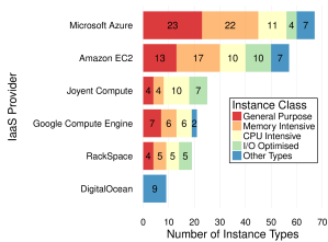
Figure 1: On-demand instance types (Linux) offered by major IaaS vendors.

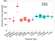
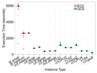
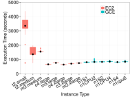
(a)	(b)	(c)

Figure 2: The execution times on various VM instances of AWS and Google of: (a) a memory-intensive application; (b) a CPU-intensive application; and (c) another CPU-intensive application. Instances from each provider are sorted from left to right in increasing instance hourly cost.

The box plots in Figure 2 represent the distributional spread of execution times of 3 different applications across a variety of instance types of Amazon EC2 and Google GCE. Figure 2(c), of a CPU-intensive application, reflects the least variability in performance levels and seems more predictable for GCE instances. The same pattern is observed across EC2 instances except the T2 series showing the highest execution time across all other nodes.

For this CPU-intensive application, c4.xlarge ($0.232/h), c3.xlarge ($0.239/h) and m3.xlarge ($0.280/h) with variable prices are performing at a very similar level, as shown in Figure 2(b). Moreover, GCE’s n1cpu4 and n1s4 show similar performance to the equivalent EC2 instances, and n1cpu8 ($0.215/h) is performing better than the expensive and predictable performing EC2 m3.xlarge ($0.280/h). On the other hand, c4.large ($0.116/h)is performing better than c3.xlarge at a much lower cost.

Figure 2(c) reflects the same trend for the T2 series as seen in Figure 2(b). A consistent performance with a negligible different in median values is observed among all GCE instances. In other words, the selection of a more expensive option does not lead to improved performance in terms of execution time.

Figure 2(a) illustrates performance variability in executing a memory-intensive application on different instance types of variable computational capacity. Contrary to previous results, the T2 series is shown as the most predictable with less variability in terms of performance. In comparison with GCE, n1s1 shows less variance in performance and offers the best execution time compared to all GCE nodes as well as a most expensive EC2 node (c4.xlarge). On top of that, n1S1 ($0.036/h) and T2 instances ($0.026-$0.052/h) are the cheapest of all. Finally, a striking observation is the poor performance of m3.medium for both executions.

The following observations can be drawn from the above discussion. The selection of an instance type based on descriptive information cannot guarantee the best fit in terms of cost and performance trade-offs. The distributional spread of results highlights the intrinsic uncertainty related to instance performance, contributing to the complexity regarding the selection of suitable instance. There are some external factors that can influence this performance such as the scheduling policy, machine age, provider-specific incentives etc. Therefore, nodes with similar capacity/specifications are difficult to compare.

Classified categories of instance types do not reflect the real performance behaviour of any application due to different architectures and the unique workload patterns of that application. Similarly, superficial knowledge about the application cannot guarantee the expected performance over different instance types.

In such decision-making situations, machine learning (ML) has potential to underpin intelligent and data-grounded Decision Support Systems (DSS). Indeed, ML-aided DSS have been demonstrated to provide behavioural and performance insights about application and deployment setup necessary to make optimal decisions, e.g. [41, 9, 20, 1]. A traditional ML approach follows the general steps of: collecting data, generating a learning model, fitting the model on training data, and assessing its accuracy on test data. This is a well established, albeit lengthy, process. However, a common assumption in this traditional learning setting is that the test and training data sets are drawn from the same distribution (say, performance of a certain cloud provider’s VMs using a particular application). If the distribution changes, such assumption no longer holds and, consequently, there needs to be a lengthy process of rebuilding the model. In our context, this means commissioning a new set of benchmarks that costs time and money.

This presents a significant challenge for ML-based decision support in multi-cloud environments, where different architectures and varying deployment setups across different cloud providers lead to significant changes in data distribution as well as feature space. Therefore, in a real world scenario, conducting such experiments is time-consuming and requires considerable cost and time for data collection and model generation.

This paper focuses on enhancing the learning efficiency of ML-aided DSS to assist application-specific decisions across different cloud providers. In this paper, we propose a novel Transfer Learning (TL) assisted scheme leading to substantial reduction in the training overhead by making use of existing knowledge. Quantitatively, we observed a reduction of approximately 60% in learning time and cost by transferring existing knowledge about an application and/or a cloud platform in order to learn a new prediction model for another application or cloud provider. The proposed scheme has the potential to deal with the challenge of model generation when data distribution or feature spaces differ between source and target domains.

Contributions

Our main contributions are as follows:

• We design and implement Tamakkon, a two-mode TL scheme that identifies the type of knowledge to be transferred across domains. We utilize a subset of well-established machine learning approaches, namely Multiple Polynomial Regression (MPR), Support Vector Regression (SVR) and Random Forests (RF). We believe this to be a novel application of TL for decision support in cloud computing.

• We present a methodology to measure similarity among different data sets in order to identify the source application and its learned data that can be used as a source of knowledge for generating a prediction model for a target application, and, additionally, to avoid negative knowledge transfer.

• Through extensive experimentation, we apply Tamakkon on different applications and cloud providers. We efficiently generate a learning model between varying application and IaaS domains, reducing the learning cost (of cloud resources and time) by 60%.

Novelty against the state of the art

Tamakkon has many unique features making it different from other similar research [49, 1, 46]. First of all, Tamakkon is based on transfer learning approach and makes use of the existing model as well data to reduce the cost and time involved for model generation and large-scale data collection. Secondly, Tamakkon works across different applications as well as cloud providers. Furthermore, a range of models are offered and the generated models result in reduced prediction errors. Moreover, the framework is extensible and new models can be added as base learners, if needed.

2.   Background on Transfer Learning (TL)

The general goal of TL is to use previously learned knowledge to solve a problem in an unseen environment or in a faster or better way. TL extracts knowledge from one or more source domains and source tasks, and applies that knowledge to achieve a task in a target domain. Given a source domain $D_{S}$ and source task $T_{S}$, a target domain $D_{T}$ and target task $T_{T}$, TL aims to improve the prediction function of $D_{T}$ using the knowledge in $D_{S}$ and $T_{S}$ considering that $D_{S}$ has some similarity with $D_{T}$ and $T_{S}=T_{T}$ or $T_{S}\neq T_{T}$. This process of achieving the target task by learning from the source domain and source task is illustrated in Figure 3.

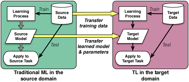
Figure 3: An overview of the TL process.

TL is categorized into two sub-types: inductive TL aims to improve the learning of a target predictive function with the help of a source task, considering that the source and target domains are the same but the tasks differ; transductive TL aims to improve the learning of a target predictive function with the help of knowledge from a source domain, where source and target domains may or may not be different but the tasks are the same.

The literature offers different approaches of transferring knowledge between two domains [36]: The instance knowledge transfer approach is applied by re-weighting some portion of source data to be used in the target domain and iteratively measuring the model fitness for target task learning [31, 12]. The feature representation knowledge transfer approach requires identification of good features that can reduce the differences between source and target domains in order to minimize model error and domain divergence [40, 3]. The parameter knowledge transfer approach is applied with an assumption that the source and target tasks share some parameters or prior distributions of the hyper-parameters of the models [28, 7]. The relational knowledge transfer approach deals with TL problems in the relational domain. TL has been applied to many real-world applications, mostly in the fields of classification of images, verbal sentiment, software defects, as well as medical tomography [8]. TL for regression tasks is a less researched area, however, some notable efforts have been made, e.g. [37, 18, 10].

3.   Tamakkon: A TL-assisted DSS

Our goal is to enhance the efficiency of intelligent DSSs in order to make data-driven and application-specific decisions in cross-cloud environments, i.e. those spanning more than a single provider. We believe that efficiency can be achieved by reducing the training overhead through making use of existing knowledge in the form of experiential data sets, significant predictive features, and prediction models and their parameters. We devise a TL-based approach to assist in efficient model generation by transferring learned knowledge from a related domain. The proposed approach is designed specifically for deployment and migration decisions in at the IaaS level.

Our approach is a semi-supervised transductive TL technique that allows the contribution of auxiliary target data for model generation. Semi-supervised learning is used due to its ability to learn with a little amount of labeled data, reducing the required amount of training data for the target domain, which is one of the key concerns of model generation efficiency.

We now present the design and implementation of our solution (§I), and detail the algorithms underpinning the TL scheme (§II–III).

I.   System architecture

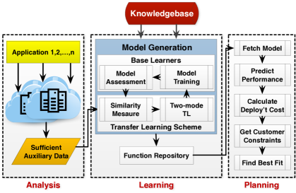
Figure 4: The architecture of Tamakkon, a novel TL-assisted cloud DSS.

The main components of the overall system architecture, shown in Figure 4, are a Knowledgebase and three phases: Analysis, Learning and Planning. The Knowledgebase is comprised of learning methods, prediction models, model parameters along with the data sets the models are derived from. The prediction models present in the Knowledgebase are generated by following the traditional ML process (i.e. train and test using cross-validation) (§I.2). The key idea of Tamakkon is to efficiently generate a prediction model for a given application and the process starts with a collection of auxiliary data (§I.3). The Analysis Phase is responsible for providing auxiliary data to be used by the Learning phase. The auxiliary data is collected by running the application on a representative set of virtual machines and profiling different matrices related to the deployment and performance of the application. The Learning Phase is the core of the architecture and is composed of four sub-modules, each performing their own unique tasks to support model generation for a target domain (i.e. application and/or provider). The model, however, is not generated from scratch by following the long steps of model fitting, but rather it is generated using Tamakkon which makes use of existing learned knowledge fetched from the Knowledgebase. Similarity Measure helps in identifying the similarity of a new domain (target) with existing ones (source). The auxiliary data is then used by the similarity measure (§II) to look for a similar application in the Knowledgebase. Based on this similarity, Tamakkon transfers existing knowledge using two-mode TL scheme, which is designed to satisfy the goal of enhancing learning efficiency and generating a prediction model for a new application. The ‘two mode’ part of the naming refers to the two possibilities of transferring learned knowledge across domains: Transfer-All and Transfer-Model. These modes present different means of transferring significant knowledge through the transfer of instance knowledge, feature space knowledge, and parameter knowledge (§III).

Together with the similarity outcome and a selected base-learner (§I.1), one of the knowledge transfer modes gets activated. The activated mode feeds in the auxiliary data as well as learned data to the base-learner which then outputs a prediction model. Model Training uses training data sets which may be composed of source and target domain data depending on the activated mode. The test data set for model assessment is comprised of the target domain’s data only. Model assessment is performed using 10-fold cross-validation and, if the output is not satisfactory, the process re-starts by fetching the next most similar application from the Knowledgebase. Finally, the accepted model is saved in the Function Repository to be used by the Planning Phase to predict future application performance. Deployment costs are generated from the predicted performance results that are then used to find the best deployment match in accordance with customer-specified constraints.

The remainder of this section details the functionality of Tamakkon modules covering base learners, auxiliary data, and similarity measurement.

I.1 Base learners

Base learners are the ML methods used to derive the initial prediction models for a source task. For Tamakkon, Multivariate Polynomial Regression (MPR), Support Vector Regression (SVR) and Random Forests (RF) are used as base learners. MPR has the ability to statistically infer and understand the relationship of response and predictor variables related to a data set. Hence, a behavioural relationship for an application can be generated with varying deployment setups. SVR attempts to obtain a function as flat as possible having an $\epsilon$-deviation from the training output [43]. SVR relies on a set of parameters such as $\epsilon$: the sensitivity to the deviation, the cost function and range of kernels, allowing it to optimize the objective function as well as the parameters of the regressive function. This allows Tamakkon to optimally adjust the hyper-parameter when fed with the different distributional training sets. RF  [16] is based on an ensemble learning approach making use of Bagging sampling and the random selection of features. The ensemble nature of RF enhances its ability to produce better prediction results. In RF, multiple decision trees (ensemble models) are generated using the randomly drawn samples. For unseen data, each decision tree takes part in the prediction process and the final prediction result is the label selected by a majority of decision trees. RF is good in accuracy and gives a better understanding of the variable importance and their correlations. Moreover, this method is considered robust to outliers as compared to other methods.

I.2 Base models

Base models are generated by following what is now deemed a traditional ML process of learning a model starting from data collection as detailed in Figure 5. This model generation is supported by Daleel’s framework [41], designed to investigate the role of ML to support application-driven decision making around the selection of instance types in a given cloud provider.

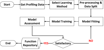
Figure 5: The model generation process.

The collected data passes through the pre-processing stage to fulfill initial assumptions about the quality of the data. Pre-processed data is then split into training and test sets and fed into an iterative process of fitting a model. The model fitting process is responsible for exploring different distributions to investigate the true relationship of a response variable with the predictors (features). The fitted model is then trained on the training data set using 10-fold cross-validation to capture the maximum variability of data and later passed on to the model assessment process to be assessed for the prediction accuracy. Further to that, the models offering satisfactory prediction capability are then stored in the function repository and, in case of unsatisfactory results, starts updating the model. Base learners are the learning methods involved in the model generation process. The significant predictors used are vCPU, RAM, Compute-units, Multithreading, Load-in-memory, Application-Type, External-file-requirement, Parallel-execution, File-size, and Execution-day. Out of these predictors, the first three represent VM configuration and rest are part of application and execution details.

I.3 Auxiliary data

Semi-supervised transductive TL, which Tamakkon is based on, requires the presence of auxiliary data for model generation. In this context, the term, “sufficient” amount of data is introduced to represent the auxiliary data requirement for the target domain to be used in Tamakkon. This is an important parameter for the approach, derived from extensive experimentation. A “sufficient amount” is identified by observing model convergence according to the change in percentage contribution of training data.

II.   Similarity measurement

A similarity measure is required to identify which of the source domains (source applications) will give the best performance on the target domains (target applications) to learn the target task (prediction model). The proposed approach leverages the Kolmogorov-Smirnov (KS) test, a non-parametric test to compare the cumulative distributions of two data sets in order to identify if the two data samples come from the same distribution.

The KS test is considered effective in comparing samples when there is no available knowledge about the common distribution of the source and target domain data. In addition, this method is sensitive to distribution and there is no restriction on the sample size which makes it useful to capture change in performance even with few samples. These properties make Tamakkon useful for different applications and machine configurations considering that often it is difficult to compare deployment settings and resource utilization between the two applications, especially when the VMs belong to different cloud providers and vary in underlying configurations.

Input: (i) Auxiliary data = $S_{aux}$

(ii) Knowledgebase data = $S_{kb_{i}}$,

where $i=1...$total number of applications

Output: (i) $D_{d}$, $D_{p}$,$D_{f}$: a similarity estimate for $S_{kb_{i}}$

(ii) Tagged knowledgebase datasets = $S_{kb_{i}}.tagged$

Initialization;

• Let $A_{j1},...,A_{jq},..,A_{jk}$ be the value in $S_{aux}$, where $A_{j1}..A_{jq}$ represents application architecture,

and $A_{jq}..A_{jk}$ represents deployment details

Let $B_{l1},...,B_{lq},..,B_{lm}$ be the value in $S_{kb_{i}}$, where $B_{l1}..B_{lq}$ represents application architecture,

and $B_{lq}..B_{lm}$ represents deployment details

Function SimilarityMeasure ($S_{aux}$, $S_{kb_{i}}$)

foreach $S_{kb_{i}}\in\{S_{kb_{1}},...,S_{kb_{n}}\}$ do

       foreach $x\in\{A_{j1},...,A_{jk}\}\cup\{B_{l1},...,A_{lm}\}$ do

             for $Two.Sample.KS.Test(x_{a},x_{b})$ do

                  Compute $p$-value $\rightarrow$ $D_{p}$

                   Compute $D^{\prime}$-value $\rightarrow$ $D_{d}$

                   if $p$-value ($D_{p}$) >0.05 then

                        $x.mark=``SAME"$

                        $x_{p}.mark=``SAME"$

                         $D_{f}=``NO"$

                  else

                        if $D^{\prime}$ ($D_{d}$) <$0.5$ then

                              $x.mark=``SAME"$

                        else

                              $x.mark=``DIFFERENT"$

                               $D_{f}=``YES"$

                         end if

                        

                   end if

                  

             end for

            

       end foreach

      $aggregate.x.mark$ for $\{A_{j1}..A_{jq}\}$ and $\{A_{jq}..A_{jk}\}$

       if value of $aggregate.x.mark$ is “SAME" for all $\{A_{j1}..A_{jq}\}$  then

            $S_{kb_{i}}.tagged=``SIMILAR"$

      else

            if  value of $aggregate.x.mark$ is “SAME" for >1/ $\{A_{j1}..A_{jq}\}$ then

                  $S_{kb_{i}}.tagged=``PARTLY-SIMILAR"$

            else

                  $S_{kb_{i}}.tagged=``NOT-SIMILAR"$

             end if

            

       end if

      

end foreach

Algorithm 1 Identification of source domain similarity

Algorithm 1 compares the probability distribution of the target application’s profiling data ($S_{aux}$) with the existing applications ($S_{kbi}$) and identifies similar distributional application(s) ($S_{kb_{i}}.tagged$) from the knowledgebase. The application(s) are tagged according to the calculated values for distributional difference ($D_{d}$) and feature difference ($D_{f}$). The KS/similarity test is applied on vector inputs ($A_{j1},...,A_{jk}$ & $B_{l1},..,B_{lm}$ ) from both source and target domain, and each vector input represents a single feature. This test outputs a p-value ($D_{p}$) and a D-value ($D_{d}$). Here p-value quantifies the probability of two samples populated from the same or a different distribution and D-value represents the difference of empirical distribution functions of two samples.

If the p-value rejects the similarity hypothesis, then the D value is evaluated to get an idea about the probability of similarity. A D-value in the range of 0.0–0.5 is considered as a measure of corresponding sample similarity from 100% to 50%. The aggregated p-values and D-values assist in deciding the similarity.

Table 1 presents the outcome of a similarity analysis based on three real world applications. The first 7 features in the table represent cloud and deployment related information and the remaining features explain application architecture. The three applications are named anonymously as A, B and C. The D-value and p-value is calculated for each feature vector taken from the source and target applications as explained in the SimilarityMeasure function. The similar features are marked as "*". An application with a high number of similar features will get a higher ranking in terms of similarity. The resulting similarity is tagged as one of three categories: 1) Similar, 2) Partly-Similar, or 3) Not-Similar.

The aggregated similar features for A and B is higher than A and C so, for application A being a target application, B would be the first choice to be used as a source of knowledge. Moreover, applications A and B have similar architectures and are tagged as Partly-Similar to each other, however application C is tagged as Not-Similar. For application C both the applications A and B are ranked the same to be used as the source, however both applications have almost no similarity at application architecture level and hence will be tagged as Not-Similar to each other.

Table 1: Pairwise similarity analysis among three applications: A, B, and C. Similarity is indicated by p- and D-values, which are calculated using the KS method for cloud, deployment and application specific features.

	A & B		A & C		C & B
Feature	D-value	p-value	D-value	p-value	D-value	p-value
vmtype	0.4082 *	2.20E-16	0.3986 *	2.20E-16	0.662	2.56E-07
vcpu	0.4063 *	2.20E-16	0.431 *	2.20E-16	0.0662 *	2.56E-07
ecu	0.4063 *	2.20E-16	0.431 *	2.20E-16	0.0662 *	2.56E-07
ram	0.4063 *	2.20E-16	0.431 *	2.20E-16	0.0662 *	2.56E-07
day	0.0804 *	2.32E-16	0.0926 *	2.20E-16	0.173 *	2.56E-07
subm. time	0.4063 *	2.20E-16	0.431 *	2.20E-16	0.0662 *	2.56E-07
exec. time	1	2.20E-16	1	2.20E-16	0.633	2.20E-16
app. type	0.4063 *	2.20E-16	0.431 *	2.20E-16	0.0662 *	2.56E-07
multi-threading	0.4063 *	2.20E-16	0.431 *	2.20E-16	0.0662 *	2.56E-07
external files	0 *	1 **	1	2.20E-16	1	2.20E-16
loaded in mem.	1	2.20E-16	1	2.20E-16	0 *	1 **
parallel	0 *	1 **	1	2.20E-16	1	2.20E-16
file size	1	2.20E-16	1	2.20E-16	1	2.20E-16
Result	Partly similar		Not similar		Not similar

III.   The Two-mode TL scheme

This section explains the core TL algorithm, derived from extensive experimental analysis on public cloud providers and applications of varying requirements. The two modes and the respective knowledge transfer approaches are discussed here:

1. Transfer-All includes three approaches to transfer knowledge from the source to the target domain.

   1. Transferring feature representation knowledge

   2. Transferring instance knowledge

   3. Transferring parameter knowledge

2. Transfer-Model includes two approaches to transfer knowledge from source to target domain.

   1. Transferring feature representation knowledge

   2. Transferring parameter knowledge

Input: (i) Auxiliary data = $S_{aux}$

(ii-a) Tagged knowledgebase datasets = $S_{kb_{i}}.tagged$

(ii-b) $X_{sig}$ of $S_{kb_{i}}.tagged$

(ii-c) Learning Method = $M_{kb_{i}}$, where $M$ is SVR, MPR, RF

(ii-d) PredictionFunction = $f(S_{kb_{i}})$

Output: (i) PredictionFunction = $f(S_{aux})$

Function Tamakkon ($S_{aux}$, $S_{kb_{i}}.tagged$, $M_{kb_{i}}$)

foreach $S_{kb_{i}}.tagged$ do

      if $S_{kb_{i}}.tagged$ == “SIMILAR" $\|$ $S_{kb_{i}}.tagged$ == “PARTLY-SIMILAR"  then

            Set $D_{d}$ = FALSE

             if $M_{kb_{i}}$ == SVR $\|$ RF then

                  Set BaseLearner=$M_{kb_{i}}$

                   Call TrasnferAll($S_{aux}$, $S_{kb_{i}}.tagged$, $X_{sig}$, BaseLearner, $D_{d}$, $f(S_{kb_{i}})$)

            else

                  if $M_{kb_{i}}$ == MPR then

                        Set BaseLearner=$M_{kb_{i}}$

                         Call TrasnferModel($X_{sig}$, $S_{aux}$, $f(S_{kb_{i}})$, BaseLearner, $D_{d}$)

                   end if

                  

             end if

            

      else

            if $S_{kb_{i}}.tagged$ == “NOT-SIMILAR" then

                   Set $D_{d}$ = TRUE

                   if $M_{kb_{i}}$ == SVR $\|$ RF then

                        Set BaseLearner=$M_{kb_{i}}$

                         Call TrasnferModel($X_{sig}$, $S_{aux}$, $f(S_{kb_{i}})$, BaseLearner, $D_{d}$)

                  else

                        if $M_{kb_{i}}$ == MPR then

                              Set BaseLearner=$M_{kb_{i}}$

                               Call TrasnferModel($X_{sig}$, $S_{aux}$, $f(S_{kb_{i}})$, BaseLearner, $D_{d}$)

                         end if

                        

                   end if

                  

             end if

            

       end if

      

end foreach

Algorithm 2 Two-mode TL Scheme

Tamakkon works by activating one of its modes based on the inputs from similarity measurement and a base learner. If the similarity outcome select a "Similar" or "Partly-Similar" application as a source of knowledge and if the learning method is SVR or RF then Transfer-All is activated and the respective knowledge is transferred from the source application to the target application. On the other hand, if there is a “Not-similar" application and the learning method is still SVR or RF, Transfer-Model gets activated. In case of the MPR learning method, the only possibility for activation mode is Transfer-Model. We now explain each of the above approaches involved in the designed scheme.

(a) Transferring feature representation knowledge

The feature space represents specific properties related to application architecture, deployment configurations and execution details. If both the source and target domains have some similarity at the application or deployment level, the higher the chances are for generating a reasonable target-learning model using the same features as for the source model. Therefore, ‘significant’ features are transferred from the source domain to the target domain. If the feature space differs in both source and target domains due to the varying standards of IaaS offerings, mapping of similar features is required. The mapping is done manually using the shared knowledge of both domains.

(b) Transferring instance knowledge

The instance knowledge represents a sample set comprised of the selected feature space. If the source and target domains have high similarity then the instance knowledge transfer can positively contribute for the model generation of the target domain, especially when there are few sample sets available for the target domain. However, the best practice is to transfer instances in an incremental manner in order to avoid any influential effect from the source data.

(c) Transferring parameter knowledge

Parameter knowledge details the mathematical formulation of the estimation or prediction function. The parameter knowledge can be shared with the target domain in accordance with the selected base learner. If the base learner is SVR then the kernel function, tuning parameters’ learning rates, the learning-cost function and model constants are transferred. For MPR, the polynomial order along with coefficient values and any interaction terms are transferred. In the case of RF, information about the number of decision trees to be generated and a number of variables to be tried at each step are shared with the target domain.

4.   Experimental Evaluation

This section describes the overall strategy to assess Tamakkon and offers a comprehensive evaluation of the proposed scheme. Tamakkon is evaluated using two public cloud providers with three representative real-world applications. These applications differ in their underlying architectures and also their memory and CPU utilization.

I.   Evaluation strategy

Our evaluation criteria are as follows:

1. Accuracy of base models, i.e. the traditional ML approach, in terms of prediction performance using overall data and using daily subsets thereof.

2. Feasibility of our TL approach under 3 distinct different evaluation scenarios: transferring to a new application, to a new provider, and to both a new application and provider, respectively (Figure 6).

3. Time and cost effectiveness of the proposed scheme in terms of incurred cloud costs and model generation time.

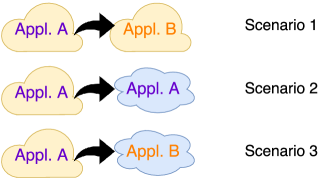
Figure 6: A high-level description of the three evaluation scenarios.

All application parameters and input are kept constant between application runs to reduce the dimensionality of the experiments. In order to collect enough data for learning purposes, we repeat a workload with a 10 minute delay between each pair of runs. This is spread over different times of the day and different days of the week to capture temporal variance. The Linux tools vmstat, glances and sysstat are used to continuously monitor resource utilization.

Different evaluation metrics were computed to assess the model accuracy, namely $R^{2}$, Residual Standard Error (RSE), Mean Squared Error (MSE) and Percentage Relative Root Mean Squared Error (%RRMSE). The metrics presented in this paper are MSE and %RRMSE. MSE is a standard measure of prediction error and we use it to assess individual model performance. %RRMSE provides a fair comparison of prediction accuracy between different learning models and data sets with variable scales by calculating a scale-independent model error relative to the actual value. As such, we use it to evaluate the performance of different models for different data sets. %RRMSE is expressed as:

$$\%RRMSE=\sqrt{\frac{1}{N}\sum_{t=1}^{N}{\frac{(y^{i}-y)^{2}}{y}}}*100$$ (1)

where $N$ is the total number of samples, and $y^{i}$ and $y$ are the predicted and actual value of application execution time, respectively. The lower the %RRMSE value is the better the model performance.

II.   Applications

We selected 3 open-source applications of different architectures and requirements of CPU and memory usage.

1. VARD is a tool designed to detect and tag spelling variations in historical texts, particularly in Early Modern English [6]. The output is aimed at improving the accuracy of other corpus analysis solutions. Vard is a single threaded Java application that is highly memory intensive. It holds in memory a representation of the full text, as well as various dictionaries that are used for normalizing spelling variations. Vard is considered a pre-processor tool to other corpus linguistic tools such as keyword analysis, semantic tagging and annotations etc.

2. smallpt is a global illumination renderer written as a multi-threaded OpenMP application and, as such, is considered CPU intensive. The application performs unbiased Monte Carlo path tracing to calculate the amount of light reaching different points in a given scene, offering features such as anti-aliasing, soft shadows, and ray-sphere intersection. For this research we selected a box scene that is constructed out of nine very large overlapping spheres.

3. ItemRecommender uses a collaborative filtering technique in order to recommend similar items, as identified using log-likelihood similarity. ItemRecommender is written as a single-threaded Java based program, and uses the MovieLens dataset collected and maintained by GroupLens. The dataset is comprised of 10 million ratings of 10,000 movies by 72,000 users. This is used to to recommend movies to a user based on the preferences of other users. The program takes every other person who has reviewed at least 5 movies in common with the user and calculates the Pearson correlation between these 2 users. Accordingly, weights are calculated and converted to numerical values to be assigned to the user’s scale and finally the recommendations are listed after sorting.

III.   Cloud infrastructure

For our target cloud providers we use Amazon EC2 and Google GCE, two of the major providers in the IaaS market. From each, we selected a subset of their on-demand (i.e. pay-as-you-go) Linux instance types deemed suitable to run the aforementioned applications. These instance types are summarized in Tables 2-3.

Table 2: Computational specifications of EC2 instances.

Series	Instance	vCPU	ECU	RAM	Storage	Price
	Type			(GiB)	(GB)	($/h)
T2 (General	t2.small	1	Var.	2	20	0.026
Purpose)	t2.medium	2	Var.	4	20	0.052
M3	m3.medium	1	3	3.75	4(S)	0.070
(General	m3.large	2	6.5	7.5	32(S)	0.140
Purpose)	m3.xlarge	4	13	15	32(S)	0.280
C4	c4.large	2	8	3.75	20	0.116
(Compute	c4.xlarge	4	16	7.5	20	0.232
Optimised)	c3.xlarge	4	14	7.5	32(S)	0.239

Table 3: Computational specifications of GCE instances.

Series	Instance	vCPU	GCEU	RAM	Storage	Price
	Type			(GB)	(GB)	($/h)
Standard	n1-standard-1	1	2.75	3.75	16	0.036
Type	n1-standard-2	2	5.5	7.5	16	0.071
	n1-standard-4	4	11	15	16	0.142
High Mem.	n1-highmem-2	2	5.5	13	16	0.106
High	n1-highcpu-2	2	5.5	1.8	16	0.056
CPU	n1-highcpu-4	4	11	3.6	16	0.118
	n1-highcpu-8	8	2.2	7.2	16	0.215

Both Amazon EC2 and GCE provide a differentiated series of instance types, catering to different application needs (e.g. compute-intensive, memory intensive, I/O-intensive, and so on). Each series contains a number of instance types offering different setups of computational resources. From EC2 we targeted the General Purpose T2 and M3 series. In addition, the Compute Optimized series is also selected with three representative instance types. Similarly, from GCE we targeted the Standard Type series instances. In addition, we selected the High CPU series as well as the High Memory series in order to evaluate varying combinations of resource capacities over a relatively wide price range.

All instances used run 64-bit Ubuntu Linux of different capacities as shown in Tables 2–3. GCE differs from Amazon-EC2 in various aspects such as the pricing scheme, VM configuration measurement units and compute units. Amazon charges on an hourly basis for VMs; in contrast, Google charges a minimum of 10 minutes per VM. Both providers have non-standard categories to offer the pool of VM’s computational power and units. The Google compute engine unit (GCEU) is an abstraction of compute resources. According to Google, 2.75 GCEUs represent the minimum power of one logical core. Amazon uses the term ‘ECU’ as a computation unit to express the CPU capabilities of its various compute offerings. The capacity unit for measuring the disk size, machine type memory, and network usage are calculated in gigabytes (GB) for each EC2 instance of Amazon. In contrast, GCE uses gibibyte (GiB) as a measuring unit for describing configurations of the VMs. It is very hard to make a 1:1 comparison with such non-standard and sometimes vague descriptions about the computational units. This creates a difference in terms of the feature space at the domain level. Moreover, some of the information, such as details of parallel workload on VMs, scheduling algorithms and how GCE virtual cores are pinned to physical cores, is not provided by the public cloud providers. So, users of IaaS cannot perceive any collocation or interference effect on their running application. The proposed approach transcends these problems and deals with such differences at the feature space level by mapping of similar features.

5.   Results

I.   Overall accuracy of base models

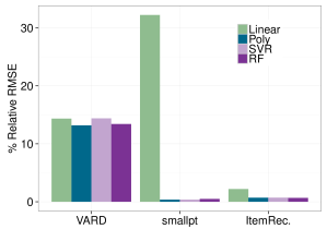
Figure 7: %RRMSE comparison of Linear, Polynomial, SVR and RF based models generated for VARD, smallpt & ItemReccomender.

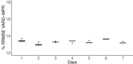
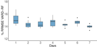
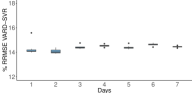
Figure 8: Model error (%RRMSE) to assess per day prediction accuracy of three base models of VARD application over the span of 7 days. The models displayed from left to right are: MPR, RF and SVR.

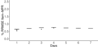
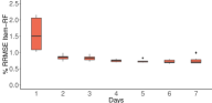
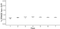
Figure 9: Model error (%RRMSE) to assess per day prediction accuracy of three base models of Item Recommender application over the span of 7 days. The models displayed from left to right are: MPR, RF and SVR.

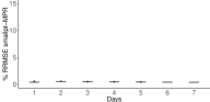
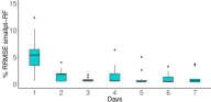
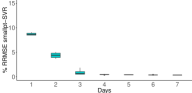
Figure 10: Model error (%RRMSE) to assess per day prediction accuracy of three base models of smallpt application over the span of 7 days. The models displayed from left to right are: MPR, RF and SVR.

Base models are generated using a traditional ML approach as explained in Section I.2 and a range of ML methods are involved in this process. The generated models for each application are compared with each other in order to assess the prediction accuracy. Figure 7 displays the %RRMSE of multiple prediction models for three applications as bar plots. For ItemRecomender, the prediction errors of MPR, SVR and RF-based models are of very similar error values, all being quite low (<0.72%). Similarly, MPR, SVR and RF-based models for smallpt are the ones with the lowest model error across (<0.41%). However, the same prediction pattern can be observed for Vard with values for MPR, SVR and RF-based models of 13.300%, 14.459%, and 13.472%, respectively, a little higher compared to smallpt and ItemRecomender specific models. The low %RRMSE values for these generated models indicate considerably reduced prediction error. In contrast, the linear model has a slightly higher error rate for Vard and ItemRecommender and a much higher one for smallpt, indicating that this is a poor model in terms of prediction accuracy.

We now explore the variance of model performance on a daily basis to assess the amount of sufficient data needed for accurate predictions. MPR, SVR, and RF based models are also evaluated to assess per day prediction accuracy for three applications, as shown in Figures 8–10. The box plots show the spread of %RRMSE values (y-axis) for 7 days of data where each entry is a result of 10-fold cross-validation.

The left plot in Figure 8 displays the prediction error of the MPR-based model for Vard with a minor variability at a day level. The error becomes more consistent with the addition of more data samples for each day and the majority of data samples are gathered around the third quartile and the first quartile for day1 and day2, respectively. The variability at distributional level gives an indication of performance variation at the VM level, investigated in more detail below. The MPR-based model for the item recommender in Figure 9 shows very low error with consistent prediction results for each day where most of the data samples are lying around the median. The left plot in Figure 10 represents the model error of the MPR-based model for smallpt and surprisingly a lowermost error rate is observed with very steady predictions for each day. The low error rates confirm that the model is able to capture maximum data variability with accurate prediction for the majority of data samples.

On the other hand, RF-based models are displaying a common pattern in all boxplots, as shown in the middle plots of Figures 8–10. A big drop in the model error is observed from day 1 to day 2 and minor drops from day 2 onwards. An interesting observation is the variability pattern for RF-Vard which is similar to MPR-Vard and providing further evidence of our assumption about significant performance fluctuation. For the RF-based model for ItemRecommender, the middle plot in Figure 9, we observe a consistent decline for %RRMSE with a narrow spread at quartile ranges and the median values are nearly aligned with the MPR-based model. The middle plot in Figure 10 shows a contrasting behaviour (RF-smallpt) compared to MPR-smallpt. The error values are spread across different quartiles on a wide range for day1 and %RRMSE keeps reducing until day 3 and then the median is consistently at the same level for the rest of the days.

Similar to MPR-Vard and RF-Vard, SVR-Vard has the same variable pattern for model error, as shown on the right in Figure 8. Contrary to RF-Vard, the error spread in SVR-Vard is narrow and the majority of data samples are gathered around the median. The model error for the SVR-based model for ItemRecommender (right plot in Figure 9) is almost the same as for the MPR based model, making it more consistent for prediction accuracy. Finally, the plot for smallpt as shown in Figure 10 displays the highest model error (>9) for day 1 with this gradually decreasing down to less than 1 by day 3 and then this is consistent until day 7. All three base learners are showing similar results with respect to different applications and presenting comparable prediction performance. Overall, MPR is converging to a lower error rate with just a day sample and has less variable prediction performance. SVR also has nearly the same pattern and converges quicker to a lower error value for two of the applications (Vard and ItemRecommender), however, there is not much evidence regarding giving a better performance with more data samples. RF, on the other hand, is more variable in terms of spread and offers better results with more data samples.

II.   Feasibility and assessment of the approach

We now assess the ability of Tamakkon to enhance learning efficacy across domains. We discuss each evaluation scenario (Figure 6) in turn.

II.1 Scenario 1: Cross-application

This first evaluation is to ascertain whether Tamakkon is able to satisfy the objective of enhancing the learning efficiency in a cross-application scenario, which could be explained as such: A model for application B can be generated to predict its performance on cloud X using the learned knowledge of application A having a model to predict its performance on cloud X.

Table 4 displays the %RRMSE of the MPR, SVR and RF-based models for this scenario, where the left most column indicates the source applications with respect to target applications listed in each column. The source applications are used as the source of knowledge and Tamakkon activates the required transfer learning mode according to similarity outcomes. Each cell value in the table is the %RRMSE value for each model, except highlighted cells which correspond to the model performance when Tamakkon is compared to the base model. The column labeled as ‘smallpt’ is referred to as column1 (c1) and so the base model values for smallpt are listed in column1 x row1 (c1r1) and so on. Here the term base model indicates the model that is generated using traditional machine learning methods (section:I.2), and training and test data sets are drawn from the same application data for which the model is generated.

C1 displays the prediction error of models generated for smallpt (target application). Vard and ItemRecommender are considered as source applications and have no similarity at application level resulting in activation of Transfer-Model. This is the case when the model specifics, as well as parameters, are used to train a model for the target application. The %RRMSE displayed in c1r2 and c1r3 are the prediction errors of the models generated by Tamakkon using the knowledge from Vard and ItemRecommender, respectively. The transferred models are performing the same as the base models (c1r1) and a negligible difference is observed for the model errors. The percentage difference for MPR-based models is 0.002%-0.008%, for SVR the range is 0.006%-0.008% and for RF the difference is 0.089%.

C2 represents the model results for Vard being a target application and smallpt (c2r1) and ItemRecommender (c2r3) as the source, where Vard shows partial similarity with the later source resulting in the use of the Transfer-All mode (section: III). The observed difference of model error for MPR is 0.008%-0.015%, SVR is 0.029%-0.022% and RF is from 0%-0.052%.

The right most column (c3) follows the same output trend, where ItemRecommender is the target application with smallpt and Vard as a source. The % difference of RRMSE values (c3r1, c3r2) for MPR, SVR and RF-based models is 0.002%-0.025%, 0.001%-0.002% and 0.024%, respectively.

Summary: The overall model error observed among all models is in range of 0%-0.089% which shows that a learning model can be successfully generated using learned knowledge from similar applications. Moreover, the results confirm the applicability of knowledge transfer approaches in a cross application scenario. In addition, teh results also justify the feasibility of SVR, MPR and RF as base-learners to generate a learning model under Tamakkon.

Table 4: Scenario-1: %RRMSE for cross-applications on EC2. Transparent cell values represent the model error using Tamakkon where the source applications serve as a source of knowledge for the target application. Highlighted cell values represent model error for three application-specific base models.

		TARGET
		smallpt	Vard	Item Rec.
SOURCE		MPR-B 0.369186	MPR- 13.3162	MPR- 0.7119354
	smallpt	SVR-B 0.37245	SVR- 14.48187	SVR- 0.7197244
		RF-B 0.408157	RF- 13.41974	RF- 0.6699096
		MPR- 0.3611638	MPR-B 13.30073	MPR- 0.684563
	Vard	SVR- 0.3658111	SVR-B 14.45976	SVR- 0.71643316
		RF- 0.4978552	RF-B 13.47269	RF- 0.6699096
		MPR- 0.3720985	MPR- 13.30905	MPR-B 0.709919
	Item Rec.	SVR- 0.3748514	SVR- 14.48974	SVR-B 0.717718
		RF- 0.4978552	RF- 13.41974	RF-B 0.654587

II.2 Scenario 2: Cross-provider

The second evaluation aims to ascertain whether Tamakkon is able to satisfy the objective of enhancing the learning efficiency in a cross-provider scenario, i.e. where the same application needs can be run on on different cloud providers. This is represented by the following example scenario: A model for application A can be generated to predict its performance on cloud Y using the learned knowledge of the same application having a model to predict its performance on cloud X.

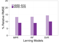
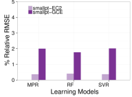
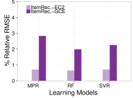
(a)	(b)	(c)

Figure 11: Scenario-2: Model error for (a) Vard, (b) smallpt, and (c) ItemRecommender. Learning models are aligned on x-axis and each set of bars represents the error of applying the same model on different cloud providers.

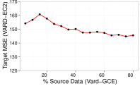
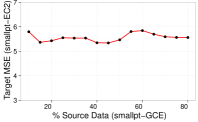
Figure 12: Scenario-2: The effect of instance knowledge from a source in improving the model in a target domain (i.e. reducing its MSE).

The data collected from the two cloud providers involved – EC2 (source) and GCE (target) – differ in feature space due to varying configuration settings at the VM level.

Each plot in Figure 11 presents the model performance of each application on GCE where the same application’s data on EC2 is used as the source of knowledge by Tamakkon. Moreover, these plots show the associated error rate of the transferred model. According to the similarity outcome, each source application in each plot is tagged as closely similar and is applicable for the Transfer-All mode with SVR as base-learner. The left plot in Figure 11 clearly depicts a lower model error for Vard-GCE for SVR, MPR and RF where %RRMSE for SVR model on EC2 is 14.459% which is comparatively higher than 10.049% on GCE. Similarly, the %RRMSE for MPR and RF on EC2 is 13.300%-13.472%, a little higher than 9.094%-8.995% on GCE. In the middle plot, MPR, SVR and RF models are performing almost the same and interestingly with a model error of less than 2% where model error for SVR, MPR and RF on EC2 is 0.3724%, 0.3691% and 0.4081%, respectively. The models are evidently performing well on GCE where the %RRMSE for SVR, MPR and RF is 2.0152%, 2.001% and 1.770%, respectively.

The right plot shows similar behaviour where the model error for the ItemRecommender on GCE is a little higher for all base learners in Tamakkon. The %RRMSE for the SVR model on GCE is 2.262% which is higher than 0.7177% on EC2. A similar trend is seen with the MPR and RF models, where the model error on EC2 is 0.7099%-0.654% which is a little lower than 2.836%-1.987% on GCE.

Furthermore, there are some surprising findings: Tamakkon results in significant reduction of model error compared to base models. For this result, the model accuracy metric is MSE as we are presenting diagnostics for one model with a particular data set. The reduced MSE is observed in two cases. First, this is observed when Vard-GCE instance knowledge is used as part of Transfer-All mode to generate a prediction model for Vard-EC2. SVR is used as the base-learner and Vard-GCE instance data is used as source knowledge. The top plot in Figure 12 describes the effect of instance data of source application (Vard-GCE) at the model training for predicting Vard-EC2 performance. The horizontal axis indicates the percentage use of source instance data mixed with the auxiliary target data, and the y-axis indicates the MSE value of test data. The MSE value is observed to consistently decrease on each percentage increase of source data. The MSE value of the base model is 177.960, which is far higher than the values seen in the graph. The lowest MSE by Tamakkon is 144.822 for Vard-EC2.

In the second case, a reduction in MSE is observed when smallpt-GCE instance knowledge is used as part of Transfer-All mode, with SVR as the base-learner, to generate a prediction model for smallpt-EC2. The results are presented in the bottom plot of Figure 12. As opposed to the above trend, we do not observe a continuous reduction of MSE. Nonetheless, some lower bounds are observed. Most importantly, the use of source instance data is able to maintain a continuous reduced MSE compared to 9.746 as the base model MSE.

Summary: The results confirm the positive influence of transferred knowledge, validating the assumption of applying a TL approach. The experiment also shows that it is possible and feasible to make use of existing knowledge to increase model accuracy. The applicability of this approach is clearly evident in this cross-provider scenario. Furthermore, the reduced model error shows the sensitivity of prediction models to capture data variation on different distributional data.

II.3 Scenario 3: Cross-application & Cross-provider

The final evaluation aims to identify whether using Tamakkon helps in providing deployment decisions across different applications and different cloud providers: in other words, is Tamakkon able to enhance learning efficiency in a cross-application, cross-provider scenario where both (a) source and target applications are different, and (b) source and target providers are different. This is illustrated by the following scenario: A prediction model can be generated for the performance of application B on cloud Y using the learned knowledge of the performance of application A on cloud X.

Again, this evaluation involves EC2 and GCE. Source knowledge is transferred based on the fact that there is little or no similarity neither at application nor cloud provider level.

Table 5 summarizes the results when applications on GCE are using existing knowledge of different applications on EC2. The results for cross-application cases (highlighted in grey) are excluded from this table as already discussed in II.2. Each cell value in the table illustrates the %RRMSE value for each model and is assessed on the test data from target application only. Under this scenario, the models are compared with each other to assess the model error for different base learners as well as evaluated for prediction accuracy on target application in comparison of the source application.

Considering smallpt-GCE as a target with Vard-EC2 (c1r2) and ItemRecommender-EC2 (c1r3) as source the percentage difference of model error for MPR-based models is 0.01%, for SVR-based models the difference is 0.003% and for RF-based models the error difference is 0.092%. Similarly, Vard-GCE as the target application has the prediction models having a model error difference of 0.060%, 0.028% and 0.263% for MPR, SVR, and RF, respectively. It can also be observed that the models generated for Vard-EC2 are presenting a better performance for Vard-GCE with reduced %RRMSE. The right most column displays values for ItemRecommender-GCE, where Vard-EC2 and smallpt-EC2 are considered as the source of knowledge. The %RRMSE difference for MPR, SVR and RF-based models is 0.085%, 0.055%, and 0.158%, respectively. This shows that Tamakkon is able to achieve reasonably accurate model generation using knowledge of a source domain and task that have no similarity at the cloud or application level. This also shows that a good feature representation can reduce domain differences even if the domains have some heterogeneity at the cloud provider level.

Summary: Perhaps not surprisingly, transferring knowledge across both application and cloud provider differences is not always successful however. Hence, this particular application of transfer knowledge is an area of future research.

Table 5: Scenario-3: %RRMSE for cross-provider, here target applications are listed in columns and source in rows. Each cell value represents the model error for three models (MPR, SVR and RF) when the source domain is EC2 and served as a source of knowledge for model generation on GCE (target domain).

		TARGET
		smallpt-GCE	Vard-GCE	Item Rec.-GCE
SOURCE			MPR- 9.094947	MPR- 2.836855
	smallpt-EC2		SVR- 10.04975	SVR- 2.26189
			RF- 8.995541	RF- 1.9887718
		MPR- 2.011354		MPR- 2.75103
	Vard-EC2	SVR- 2.011354		SVR- 2.31769
		RF- 1.862442		RF- 2.147283
		MPR- 2.001243	MPR- 9.161341
	Item Rec.-EC2	SVR- 2.015265	SVR- 10.07811
		RF- 1.770105	RF- 9.258656

III.   Time and cost effectiveness

In addition to the above validation of our applied TL scheme, the approach is been evaluated for time and cost-effectiveness. A key feature of Tamakkon is the utilization of existing knowledge in the form of the learned model (Transfer-Model) and data instances (Transfer-All). This results in a reduction of time to generate a model from scratch. Additionally, utilizing existing data instances reduces the cost required to collect a large amount of data for a new application.

Model generation on its own incurs a variable amount of time at each stage: data pre-processing, feature selection, model calibration, parameter tuning, model training, and assessment [15]. Figure 13 illustrates the approximate time needed to generate a learning model by using traditional model generation methods in comparison to transfer learning using our approach. MPR requires additional efforts to identify a best fit model and to examine non-linear curve fitting of multiple predictors with a response variable; i.e. very transparent in ML terms. Therefore, it incurs the highest time ($\approx$900 minutes) for model generation involving frequent human intervention to evaluate outcomes at each sub-stage. SVR comes second ($\approx$ 420 minutes) where the majority of the time is used for parameter tuning. RF takes less time ($\approx$300 minutes), and is observed to offer better understanding of the relationship of predictors with the response variables as compared to SVR.

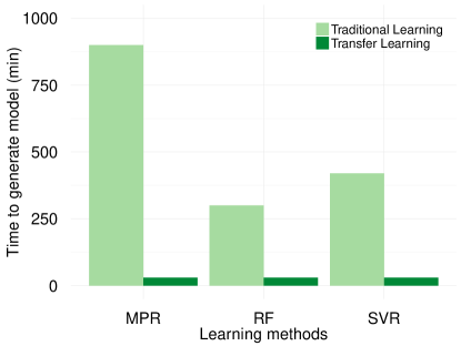
Figure 13: The time taken to generate models using traditional ML and TL.

It is clearly seen from Figure 13 that TL can reduce the significant effort of model generation. The time for TL includes pre-processing of new data, similarity measurement, model transfer, training, assessment and any human intervention to check through the process. Model accuracy is a proxy metric for model generation time and training cost: the lower the model error, the less time and cost required to train the new model as only a subset of the target application data is used to train the generated model. Such saving brought on by the use of existing knowledge is potentially very significant as collecting data to train a model is a lengthy and costly process in terms of costs needed for cloud resources to collect data samples. Overall, model training is made more efficient by saving 60.12% of the required cost and time. Specifically, we were able to reduce VM usage for the purpose of data collection for a single application from 168 hours to 67 hours. This translates to saving $92.33 out of $153.88 on 8 EC2 VMs. Similarly, on GCE, a cost of $53.323 from a total of $88.872 was saved on one single experiment comprised of 7 nodes.

6.   Related Work

A big challenge in cloud computing stems from the wide variety of technologies, APIs, and terminologies used [14]. Furthermore, uncertainty associated with how these services are managed (e.g. scheduling algorithms, load balancing policies, co-location strategies, etc. [32, 41, 29]) add a black-box effect to this complexity.

Thus, providing customers with realistic and application-specific deployment decisions is an important and complex goal. In this decision process, application requirements are being matched with cloud resources. Broadly speaking, there are two approaches to such a decision-making process, which we review below.

Metric-based solutions rely on representing cloud resources and their capabilities in a certain way, such as using standardized KPIs (e.g. [19, 5, 38, 17]) or through benchmarking (e.g. [30, 45]). The former method results, despite all efforts, in an outdated and reductive representation due to the sheer breadth and proliferation of the cloud computing market. The latter method avoids this through persistent benchmarking in an attempt to capture irregularities and attain a detailed and up-to-date performance profile for each different cloud resource type. This of course comes at a high operational cost. Moreover, a disadvantage of both methods is that they are based on application-agnostic ranking and not on knowing how the application will actually perform on a given infrastructure.

Application models focus more on the other part of the matchmaking decision process: application requirements. Examples include vendor-independent ontologies (e.g. [39, 24]) and model-driven engineering (e.g. [4, 34, 22]). These solutions are heavily dependent on fine-grained information from domain experts, analysts and decision makers to get complete knowledge of business models and company strategies [23]. As such, a designer must be aware of the impact of decisions, alternative decisions, actor interactions, dependencies, and processes while designing workflows and architectural models. Such processes require significant developer experience and time to follow domain-specific design principles.

ML-based methods are also starting to emerge. Such methods aim to gain the best of both worlds by using experiential data (as benchmarks do) to model application behaviour on different deployment setups. A prominent trend in such studies is to focus on data analytics and MapReduce-style applications [48, 20, 21, 9], due to their operational footprint and having a recurrent workload pattern which is relatively easy to model. However, a common overhead here is training: significant data and time (which translates to cloud costs) are needed to train a model. Therefore, more recent efforts focus on reducing the learning cost. Ernest [46] offers a performance prediction for analytic applications, and uses an optimal experimental design technique to select useful training point for model generation. This, however, requires extensive evaluation to optimize the cost-performance trade-off. CherryPick [1] uses optimization and encoding methods to obtain a near optimal solution and to narrow down the search space. However, the solution is designed for recurrent analytic applications and is restricted to provide only one solution as an optimal choice. Tamakkon, on the other hand, is not designed for any particular application domain and can optimize the cost-performance trade-off for different ranges of VMs. Paris [49] uses hybrid offline benchmarking to generate sufficient workload fingerprints to obtain a cost-performance trade-off. Though, combining synthetically generated data with real-world data will typically results in the reduction of prediction accuracy as is evident from the low prediction accuracy reported in the Paris paper as compared to that of Tamakkon.

A final note: Several recent works used ML to look into the variation of auctioned cloud resources (as opposed to on-demand ones), namely AWS Spot, e.g. [25, 50, 47]. However, this has been proven to be a relatively trivial optimization problem [42] and is not of interest to our work.

7.   Conclusion

Decision making in cloud environments is a challenging task due to the wide and ever expanding variety of IaaS service offerings. A customer entering such diverse market is likely to be confused with the range of choices on offer and without much knowledge about the selection criteria. A decision support system supplemented with traditional machine learning methods is therefore a very attractive service for cloud users. However, this inevitably comes with a significant learning time and monetary cost for making decisions specific to each application and cloud infrastructure.

In this paper we present Tamakkon, a novel solution to increase the efficiency of ML-assisted DSS to make application-specific decisions in a cross-cloud environment. The solution makes use of existing knowledge, transferring such knowledge to be used for other applications and/or cloud infrastructures. More specifically, this work applies TL to identify the type of knowledge to be transferred and details a methodology to identify similarity between different sources of knowledge. Tamakkon is not using source pre-trained models. Instead, it is training a function over the source and target application data. This approach is evaluated from three perspectives involving two public cloud providers and three applications of varying architectures. The evaluation results are very promising and identify a significant reduction in model generation overhead (of 60%) in terms of time and cost. Thus, Tamakkon is able to enhance the capability of intelligent decision support systems to make them more cost-effective. This important contribution is also applicable for multi-cloud brokers [13] in considering a large amount of deployment options.

This work opens up a number of avenues for future research. In particular, it would be interesting to enrich the framework with supplementary learning methods including exploration of unsupervised transfer learning techniques [44]. Moreover, it would be interesting to extend the study to deal with multi-criteria decision making and to better understand the generality of this approach by expanding to other categories of applications and cloud providers.

References

- [1] O. Alipourfard, H. H. Liu, J. Chen, S. Venkataraman, M. Yu, and M. Zhang. Cherrypick: Adaptively unearthing the best cloud configurations for big data analytics. In NSDI, pages 469–482, 2017.
- [2] AppDirect. SMB cloud service adoption report, 2017.
- [3] A. Argyriou, T. Evgeniou, and M. Pontil. Convex multi-task feature learning. Machine Learning, 73(3):243–272, 2008.
- [4] B. Balis, K. Figiela, M. Malawski, M. Pawlik, and M. Bubak. A lightweight approach for deployment of scientific workflows in cloud infrastructures. In Parallel Processing and Applied Mathematics, pages 281–290. Springer, 2016.
- [5] G. Baranwal and D. P. Vidyarthi. A cloud service selection model using improved ranked voting method. Concurrency and Computation: Practice and Experience, 28(13):3540–3567, 2016.
- [6] A. Baron and P. Rayson. Vard2: A tool for dealing with spelling variation in historical corpora. In PG Conference in Corpus Linguistics, May 2008.
- [7] E. V. Bonilla, K. M. Chai, and C. Williams. Multi-task gaussian process prediction. In NIPS, pages 153–160. 2008.
- [8] V. Cheplygina, I. P. Peña, J. J. H. Pedersen, D. A. Lynch, L. Sørensen, and M. de Bruijne. Transfer learning for multi-center classification of chronic obstructive pulmonary disease. IEEE Journal of Biomedical and Health Informatics, 22(5):1486–1496, Sept 2018.
- [9] R. C. Chiang, J. Hwang, H. H. Huang, and T. Wood. Matrix: Achieving predictable virtual machine performance in the clouds. In ICAC, 2014.
- [10] K. Choi, G. Fazekas, M. B. Sandler, and K. Cho. Transfer learning for music classification and regression tasks. CoRR, abs/1703.09179, 2017.
- [11] Cloud Standards Coordination (Phase 2). Cloud computing users needs - analysis, conclusions and recommendations from a public survey. Special Report 003 381 V2.1.1, The European Telecommunications Standards Institute, Feb. 2016.
- [12] W. Dai, Q. Yang, G.-R. Xue, and Y. Yu. Boosting for transfer learning. In ICML, pages 193–200, 2007.
- [13] A. Elhabbash, F. Samreen, J. Hadley, and Y. Elkhatib. Cloud brokerage: A systematic survey. ACM Comput. Surv., 51(6):119:1–119:28, Jan. 2019.
- [14] Y. Elkhatib. Mapping cross-cloud systems: Challenges and opportunities. In HotCloud, 2016.
- [15] Y. Elkhatib. Navigating diverse data science learning: Critical reflections towards future practice. In Curricula and Teaching Methods in Cloud Computing, Big Data, and Data Science, 2017.
- [16] K. Fawagreh, M. M. Gaber, and E. Elyan. Random forests: from early developments to recent advancements. Systems Science & Control Engineering, 2(1):602–609, 2014.
- [17] A. J. Ferrer, F. Hernández, J. Tordsson, E. Elmroth, A. Ali-Eldin, C. Zsigri, R. Sirvent, J. Guitart, R. M. Badia, K. Djemame, W. Ziegler, T. Dimitrakos, S. K. Nair, G. Kousiouris, K. Konstanteli, T. Varvarigou, B. Hudzia, A. Kipp, S. Wesner, M. Corrales, N. Forgó, T. Sharif, and C. Sheridan. OPTIMIS: A holistic approach to cloud service provisioning. Future Gener. Comput. Syst., 28(1):66–77, Jan. 2012.
- [18] J. Garcke and T. Vanck. Importance weighted inductive transfer learning for regression. In ECML PKDD, pages 466–481. Springer-Verlag, 2014.
- [19] S. K. Garg, S. Versteeg, and R. Buyya. A framework for ranking of cloud computing services. Future Gener. Comput. Syst., 29(4):1012–1023, June 2013.
- [20] A. E. Gencer, D. Bindel, E. G. Sirer, and R. van Renesse. Configuring distributed computations using response surfaces. In Middleware, pages 235–246. ACM, 2015.
- [21] C.-J. Huang, Y.-W. Wang, C.-T. Guan, H.-M. Chen, and J.-J. Jian. Applications of machine learning to resource management in cloud computing. International Journal of Modeling and Optimization, 3(2):148–152, 2013.
- [22] A. Jumagaliyev and Y. Elkhatib. CadaML: A modeling language for multi-tenant cloud application data architectures. In IEEE CLOUD, July 2019.
- [23] A. Jumagaliyev, J. Whittle, and Y. Elkhatib. Using dsml for handling multi-tenant evolution in cloud applications. In CloudCom, Dec. 2017.
- [24] E. Kamateri, N. Loutas, D. Zeginis, J. Ahtes, F. D’Andria, S. Bocconi, P. Gouvas, G. Ledakis, F. Ravagli, O. Lobunets, and K. Tarabanis. Cloud4SOA: A Semantic-Interoperability PaaS Solution for Multi-cloud Platform Management and Portability, volume 8135 of LNCS, chapter 6, pages 64–78. 2013.
- [25] C. Kilcioglu and C. Maglaras. Revenue maximization for cloud computing services. SIGMETRICS Performance Evaluation Review, 43(3):76, 2015.
- [26] C. Kilcioglu, J. M. Rao, A. Kannan, and R. P. McAfee. Usage patterns and the economics of the public cloud. In WWW, pages 83–91, 2017.
- [27] M. Lang, M. Wiesche, and H. Krcmar. What are the most important criteria for cloud service provider selection? a delphi study. In ECIS, 2016.
- [28] N. D. Lawrence and J. C. Platt. Learning to learn with the informative vector machine. In ICML, pages 65–, 2004.
- [29] P. Leitner and J. Cito. Patterns in the chaos — a study of performance variation and predictability in public IaaS clouds. ACM Transactions on Internet Technology, 16(3):15:1–15:23, Apr. 2016.
- [30] A. Li, X. Yang, S. Kandula, and M. Zhang. CloudCmp: Comparing public cloud providers. In IMC, pages 1–14. ACM, 2010.
- [31] X. Liao, Y. Xue, and L. Carin. Logistic regression with an auxiliary data source. In ICML, pages 505–512, 2005.
- [32] A. K. Maji, S. Mitra, B. Zhou, S. Bagchi, and A. Verma. Mitigating interference in cloud services by middleware reconfiguration. In Middleware, pages 277–288. ACM, 2014.
- [33] J. McKendrick. What cloud computing customers want: Clarity, simplicity, support, 2014.
- [34] A. Menychtas, K. Konstanteli, J. Alonso, L. Orue-Echevarria, J. Gorronogoitia, G. Kousiouris, C. Santzaridou, H. Bruneliere, B. Pellens, P. Stuer, et al. Software modernization and cloudification using the ARTIST migration methodology and framework. Scalable Computing: Practice and Experience, 15(2):131–152, 2014.
- [35] Z. Ou, H. Zhuang, J. K. Nurminen, A. Ylä-Jääski, and P. Hui. Exploiting hardware heterogeneity within the same instance type of Amazon EC2. In HotCloud, 2012.
- [36] S. J. Pan and Q. Yang. A survey on transfer learning. IEEE Transactions on Knowledge and Data Engineering, 22(10):1345–1359, Oct. 2010.
- [37] D. Pardoe and P. Stone. Boosting for regression transfer. In ICML, pages 863–870, 2010.
- [38] P. Pawluk, B. Simmons, M. Smit, M. Litoiu, and S. Mankovski. Introducing STRATOS: A cloud broker service. In IEEE Cloud, 2012.
- [39] D. Petcu. Portability and interoperability between clouds: Challenges and case study. In ServiceWave, pages 62–74. Springer-Verlag, 2011.
- [40] R. Raina, A. Battle, H. Lee, B. Packer, and A. Y. Ng. Self-taught learning: Transfer learning from unlabeled data. In ICML, pages 759–766, 2007.
- [41] F. Samreen, Y. Elkhatib, M. Rowe, and G. S. Blair. Daleel: Simplifying cloud instance selection using machine learning. In IEEE/IFIP NOMS, pages 557–563, April 2016.
- [42] P. Sharma, D. Irwin, and P. Shenoy. How not to bid the cloud. In HotCloud, 2016.
- [43] A. J. Smola and B. Schölkopf. A tutorial on support vector regression. Statistics and Computing, 14(3):199–222, Aug. 2004.
- [44] M. Usama, J. Qadir, A. Raza, H. Arif, K.-L. A. Yau, Y. Elkhatib, A. Hussain, and A. Al-Fuqaha. Unsupervised machine learning for networking: Techniques, applications and research challenges. IEEE Access, 2019.
- [45] B. Varghese, O. Akgun, I. Miguel, L. Thai, and A. Barker. Cloud benchmarking for performance. In CloudCom, pages 535–540, Dec 2014.
- [46] S. Venkataraman, Z. Yang, M. Franklin, B. Recht, and I. Stoica. Ernest: Efficient performance prediction for large-scale advanced analytics. In NSDI, pages 363–378, 2016.
- [47] C. Wang, Q. Liang, and B. Urgaonkar. An empirical analysis of Amazon EC2 spot instance features affecting cost-effective resource procurement. In ACM/SPEC ICPE, pages 63–74. ACM, 2017.
- [48] A. Wieder, P. Bhatotia, A. Post, and R. Rodrigues. Orchestrating the deployment of computations in the cloud with conductor. In NSDI, pages 27–27, 2012.
- [49] N. J. Yadwadkar, B. Hariharan, J. E. Gonzalez, B. Smith, and R. H. Katz. Selecting the best VM across multiple public clouds: A data-driven performance modeling approach. In SoCC, pages 452–465. ACM, 2017.
- [50] L. Zheng, C. Joe-Wong, C. W. Tan, M. Chiang, and X. Wang. How to bid the cloud. In SIGCOMM, pages 71–84. ACM, 2015.