Uncertainty Modeling of Contextual-Connections between Tracklets for Unconstrained Video-based Face Recognition

Abstract

Unconstrained video-based face recognition is a challenging problem due to significant within-video variations caused by pose, occlusion and blur. To tackle this problem, an effective idea is to propagate the identity from high-quality faces to low-quality ones through contextual connections, which are constructed based on context such as body appearance. However, previous methods have often propagated erroneous information due to lack of uncertainty modeling of the noisy contextual connections. In this paper, we propose the Uncertainty-Gated Graph (UGG), which conducts graph-based identity propagation between tracklets, which are represented by nodes in a graph. UGG explicitly models the uncertainty of the contextual connections by adaptively updating the weights of the edge gates according to the identity distributions of the nodes during inference. UGG is a generic graphical model that can be applied at only inference time or with end-to-end training. We demonstrate the effectiveness of UGG with state-of-the-art results in the recently released challenging Cast Search in Movies and IARPA Janus Surveillance Video Benchmark dataset.

1 Introduction

Unconstrained video-based face recognition has been an active research topic for decades in computer vision and biometrics. In a wide range of its applications, such as visual surveillance, video content analysis and access control, the task is to match the subjects in unconstrained probe videos to pre-enrolled gallery subjects, which are represented by still face images. Although recent advances of deep convolutional neural network (DCNN)-based methods have achieved comparable or superior performance to human in still-image based face recognition [28, 20, 23, 1, 21, 26, 27, 6, 5], unconstrained video-based face recognition still remains a challenging problem due to significant facial appearance variations caused by pose, motion blur, and occlusion.

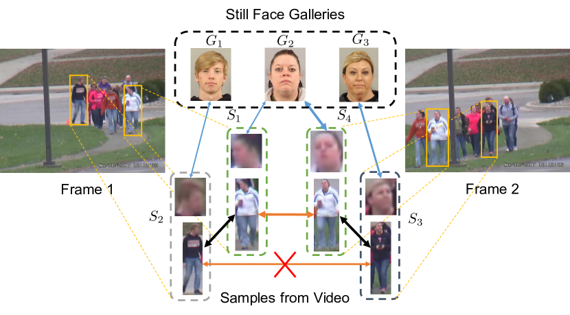
Figure 1: An example of video-based face recognition problem consisting of three still face gallery subjects and four samples from the videos. Orange arrows show positive connections from body appearance similarity. Black arrows indicate negative connections constructed from co-occurrence information. Blue arrows represent the facial similarities to the ground truth galleries. The thicker the arrows, the stronger the connections. The red cross indicates an misleading connection. A graph with fixed connections may propagate erroneous information through these misleading connections. (The figure is best viewed in color.)

To fill the performance gap between face recognition in still-images and unconstrained videos, one possible solution is to train a video-specific model with large amount of training data, which is difficult and costly to collect. Another effective idea is to leverage the well-studied image-based face recognition methods to first identify video faces with limited variations, then utilize some video contextual information, such as body appearance and spatial-temporal correlation between person instances, to propagate the identity information from high-quality faces to low-quality ones. For instance, in Figure 1, by utilizing the body appearance, we may propagate the identity information obtained from frontal face $S_{4}$ to the profile face $S_{1}$, which is very difficult to recognize individually.

The above idea has been explored using graph-based approaches [13, 7, 25]. Graphs are constructed with nodes to represent one or more frames (tracklets) of person instances and edges to connect tracklets. However, a major limitation of these approaches is that their graphs are pre-defined and the edges are fixed during information propagation. A misleading connection may propagate erroneous information. As shown in Figure 1, these methods may propagate the identity information between $S_{2}$ and $S_{3}$ based on their similar body appearance, which might lead to erroneous propagation.

To address the problem, we propose a graphical-model-based framework called Uncertainty-Gated Graph (UGG) to model the uncertainty of connections built using contextual information. We formulate UGG as a conditional random field on the graph with additional gate nodes introduced on the connected graph edges. With a carefully designed energy function, the identity distribution of tracklets is updated by the information propagated through these gate nodes during inference. In turn, these gate nodes are adaptively updated according to the identity distributions of the connected tracklets. The uncertainty gate nodes consist of two types of gates: positive gates that control the confidence of the positive connections (encourage the connected pairs to have the same identity) and negative gates that control negative ones (discourage pairs to have the same identity). It is worth noting that negative connections can significantly contribute to performance improvements by discouraging similar identity distribution between clearly distinct subjects, e.g., two people in the same frame. Explicitly modeling positive/negative information separately allows our model to consider different contextual information in challenging conditions, and leads to improved uncertainty modeling.

Our approach can be directly applied at inference time, or plugged onto an end-to-end network architecture for supervised and semi-supervised training. The proposed method is evaluated on two challenging datasets, the Cast Search in Movies (CSM) dataset [13] and the IARPA Janus Surveillance Video Benchmark (IJB-S) dataset [14] with superior performance compared to existing methods.

The main contributions of this paper are summarized as follows:

• We propose the Uncertainty-Gated Graph model for video-based face recognition by explicitly modeling the uncertainty of connections between tracklets using uncertainty gates over graph edges. The tracklets and gates are updated jointly and possible connection errors might be corrected during inference.

• We utilize both positive and negative connections for information propagation. Despite its effectiveness, negative connections were often ignored in previous approaches for unconstrained face recognition.

• The proposed method is efficient and flexible. It can either be used at inference time without supervision, or be considered as a trainable module for supervised and semi-supervised training.

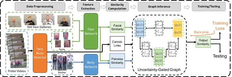
Figure 2: Overview of the proposed method. Given still face galleries and probe videos, we first detect all the faces and corresponding bodies from the videos. Faces are associated into tracklets by a tracker. Face features for galleries and tracklets, and body features for tracklets are extracted by corresponding networks. Similarities are computed from these flattened features. Facial and body similarities, together with cannot-link constrains from the detection information are fed into the proposed UGG model. After inference, the output is used for testing, or generating the loss for end-to-end training.

2 Related Works

Deep Learning for Face Recognition: Deep learning is widely used for face recognition tasks as it has demonstrated significant performance improvements. Sun et al. [26, 27] achieved results surpassing human performance on the LFW dataset [12]. Parkhi et al. [20] achieved impressive results for face verification. Chen et al. [1, 2] reported very good performance on IJB-A, JANUS CS2, LFW and YouTubeFaces [32] datasets. Ranjan et al. [21] achieved good performance on IJB-C[19]. Zheng et al. [33] achieved good performance on video face datasets including IJB-B [31] and IJB-S [14]. [5] presents a recent face recognizer with state-of-the-art performance.

Label Propagation: Label propagation [35] has many applications in computer vision. Huang et al. [13] proposed an approach for searching person in videos using a label propagation scheme instead of trivial label diffusion. Kumar et al. [16] proposed a video-based face recognition method by selecting key-frames and propagating the labels on key-frames to other frames. Sheikh et al. [24] used label propagation to reduce the runtime for semantic segmentation using random forests. Tripathi et al. [29] introduced a label propagation-based object detection method.

Conditional Random Field: The Conditional Random Field (CRF) [17] is a commonly used probabilistic graphical models in computer vision research. Krähenbühl et al. [15] is one of the early researchers to use CRF for semantic segmentation. Chen et al. [3, 4] proposed a DCNN-based system for semantic segmentation and used a CRF for post-processing. Zheng et al. [34] further introduced an end-to-end framework of a deep network with a CRF module for semantic segmentation. Du et al. [7] used a CRF to solve the face association problem in unconstrained videos.

Graph Neural Networks: A Graph Neural Network (GNN) [22, 10] is a neural network combined with graphical models such that messages are passed in the graph to update the hidden states of the network. Shen et al. [25] used a GNN for person re-identification problem. Hu et al. [11] introduced a structured label prediction method based on a GNN, which allows positive and negative messages to pass between labels guided by external knowledge. But the graph edges are fixed during testing. Wang et al. [30] introduced a zero-shot learning method using stacked GNN modules. Lee et al. [18] proposed another multi-label zero-shot learning method by message passing in a GNN based on knowledge graphs.

Most of the graph-based methods mentioned above only allow positive messages to pass in the graph, and all of them rely on graphs with fixed edges during testing.

3 Proposed Method

The overview of the method is shown in Figure 2. For each probe video, faces are detected and associated into tracklets. Initial facial similarities between gallery images and probe tracklets are computed by a still face recognizer. Connections between tracklets are generated based on the similarity of their facial, body appearances and their spatial-temporal relationships. Then, we build the UGG where these tracklets and connections act as nodes and edges. The connections between tracklets are modeled as uncertainty gates between nodes. The inference can be efficiently implemented by message passing to optimize the energy function of the UGG module.

3.1 Problem Formulation

For a video-based face recognition problem, suppose we have $C$ gallery subjects and a probe video. The faces in this video are first detected and tracked into $N$ tracklets. For each tracklet, we compute $C$ similarity scores to gallery subjects.

Suppose we are given the gallery-to-tracklet similarity $\mathbf{S}^{gt}=\begin{bmatrix}s_{li}^{gt}\end{bmatrix}\in\mathbb{R}^{C\times N}$ and the tracklet-to-tracklet similarity $\mathbf{S}^{tt}=\begin{bmatrix}s_{ij}^{tt}\end{bmatrix}\in\mathbb{R}^{N\times N}$, where $s_{li}^{gt}$ is the similarity between the gallery $l$ and the tracklet $i$, $s_{ij}^{tt}$ is the similarity between tracklet $i$ and $j$. Furthermore, a cannot-link matrix $\mathbf{L}^{tt}=\begin{bmatrix}L_{ij}^{tt}\end{bmatrix}\in\{0,1\}^{N\times N}$ is given such that

$$\small L_{ij}^{tt}=\begin{cases}1&\text{identities of tracklet $i$ and $j$ are different}\\ 0&\text{no constraint}\end{cases}$$ (1)

Here, $\mathbf{S}^{gt}$ provides prior identity information, $\mathbf{S}^{tt}$ provides the positive contextual information between tracklets and $\mathbf{L}^{tt}$ provides the negative contextual information. By combining these information, the output gallery-to-tracklet similarity is computed as

$$\small\tilde{\mathbf{S}}^{gt}=UGG(\mathbf{S}^{gt},\mathbf{S}^{tt},\mathbf{L}^{tt})\in\mathbb{R}^{C\times N}$$ (2)

where $UGG(\cdot)$ is a function based on the proposed Uncertainty-Gated Graph. In the following sections, we introduce the model in detail.

3.2 Uncertainty-Gated Graph

First, given a video with $N$ tracklets detected, a graph $\mathcal{G}=(\mathcal{V},\mathcal{E})$ is built where each node corresponds to a tracklet. Node $i$ is only connected to its neighbors $\mathcal{N}(i)$. Based on the graph $\mathcal{G}$, we define a random field $\mathbf{X}=\{X_{1},\dots,X_{N}\}$ associated to nodes $\mathcal{V}$. $X_{i}\in\mathcal{L}=\{1,\dots,C\}$ is the label variable of tracklet $i$. $X_{i}=l$ means gallery subject $l$ is assigned to tracklet $i$. We call these nodes as sample nodes.

We further add gates nodes to each of the edges in $\mathcal{E}$ attached with a random field $\mathbf{Y}=\{Y_{i\to j}^{p},Y_{i\to j}^{n}\}$. In each gate node $i\to j$, we place two gate variables, the positive gate $Y_{i\to j}^{p}\in\{0,1\}$ and the negative gate $Y_{i\to j}^{n}\in\{0,1\}$, to control the connections between tracklets $i$ and $j$.

3.2.1 Energy Function

The energy function of the UGG module is defined as

$$E(\mathbf{x},\mathbf{y}) =\sum_{i\in\mathcal{V}}\psi_{u}^{x}(x_{i})+\sum_{i\in\mathcal{V},j\in\mathcal{N}(i)}[\psi_{u}^{p}(y_{i\to j}^{p})+\psi_{u}^{n}(y_{i\to j}^{n})$$

$$+\psi_{t}^{p}(x_{i},x_{j},y_{i\to j}^{p})+\psi_{t}^{n}(x_{i},x_{j},y_{i\to j}^{n})]$$ (3)

The unary potential for tracklet $i$ is defined based on the identity information $\mathbf{S}^{gt}$ as

$$\small\psi_{u}^{x}(x_{i}=l)=-T_{gt}\cdot s_{li}^{gt}$$ (4)

where $T_{gt}$ is the temperature factor. The penalty will be low if identity information $s_{li}^{gt}$ is strong.

We also define the unary potential for the positive gate based on relationship information $\mathbf{S}^{tt}$ as

$$\small\psi_{u}^{p}(y_{i\to j}^{p}=1)=-T_{tt}\cdot s_{ij}^{tt}$$ (5)

where $T_{tt}$ is the corresponding temperature factor. Penalty of an open positive gate at edge $i\to j$ will be low if positive connection $s_{ij}^{tt}$ is strong.

The unary potential for the negative gate is defined as

$$\small\psi_{u}^{n}(y_{i\to j}^{n}=k)=\begin{cases}0&\text{if }L_{ij}^{tt}=k\\ +\infty&\text{otherwise}\end{cases}$$ (6)

for $k\in\{0,1\}$. Therefore, opening of the negative gate at node $i\to j$ is determined by the negative connection $L_{ij}^{tt}$.

The positive triplet potential is defined as

$$\small\psi_{t}^{p}(x_{i},x_{j},y_{i\to j}^{p})=\begin{cases}\alpha_{p}&\text{if }y_{i\to j}^{p}=1\text{ and }x_{i}\neq x_{j}\\ 0&\text{otherwise}\end{cases}$$ (7)

where $\alpha_{p}$ is the positive penalty. Since $y_{i\to j}^{p}=1$ means an open positive gate between tracklet $i$ and $j$, it generates positive information to nodes $i$ and $j$ if $x_{i}$ and $x_{j}$ take different labels.

Similarly, the negative triplet potential is defined as

$$\small\psi_{t}^{n}(x_{i},x_{j},y_{i\to j}^{n})=\begin{cases}\alpha_{n}&\text{if }y_{i\to j}^{n}=1\text{ and }x_{i}=x_{j}\\ 0&\text{otherwise}\end{cases}$$ (8)

where $\alpha_{n}$ is the negative penalty. Since $y_{i\to j}^{n}=1$ means an open negative gate between tracklet $i$ and $j$, it generate negative information to nodes $i$ and $j$ if $x_{i}$ and $x_{j}$ have the same label.

3.3 Model Inference

Directly looking for the label assignment that minimizes $E(\mathbf{x},\mathbf{y})$ is a combinatorial optimization problem which is intractable. Instead, similar to [15], we use the mean field method to approximate the distribution $P(\mathbf{X},\mathbf{Y})\propto\exp(-E(\mathbf{X},\mathbf{Y}))$ by the product of independent marginals

$$\small\vspace{-5pt}Q(\mathbf{X},\mathbf{Y})=\prod_{i}Q_{i}(X_{i})\prod_{j\in\mathcal{N}(i)}Q_{i\to j}^{p}(Y_{i\to j}^{p})Q_{i\to j}^{n}(Y_{i\to j}^{n})\vspace{-5pt}$$ (9)

Here $Q_{i}(X_{i})$ is the identity distribution of node $i$, $Q_{i\to j}^{p}(Y_{i\to j}^{p})$ and $Q_{i\to j}^{n}(Y_{i\to j}^{n})$ are the status distributions of positive and negative gates on edge $i\to j$ respectively.

Let $\mathbf{q}_{i}^{(t)}=\begin{bmatrix}Q_{i}(1)^{(t)}&\cdots&Q_{i}(C)^{(t)}\end{bmatrix}^{T}$ be the identity distribution vector of node $i$ at the $t$-th iteration. $\pi_{i\to j}^{p,(t)}=Q_{i\to j}^{p,(t)}(1)$ and $\pi_{i\to j}^{n,(t)}=Q_{i\to j}^{n,(t)}(1)$ be the probability of opened positive and negative gates on edge $i\to j$ respectively. Minimizing the KL-divergence $D(Q||P)$ between $P(\mathbf{X},\mathbf{Y})$ and $Q(\mathbf{X},\mathbf{Y})$ yields the following message passing updates:

1) For sample nodes, we have

$$\mathbf{q}_{i}^{(0)}=\operatorname{softmax}(T_{gt}\mathbf{S}_{:,i}^{gt} )$$

$$\mathbf{q}_{i}^{(t)}=\operatorname{softmax}(T_{gt}\mathbf{S}_{:,i}^{gt} +\alpha_{p}\sum_{j\in\mathcal{N}(i)}\pi_{i\to j}^{p,(t-1)}\mathbf{q}_{j}^{(t-1)}$$

$$-\alpha_{n}\sum_{j\in\mathcal{N}(i)}\pi_{i\to j}^{n,(t-1)}\mathbf{q}_{j}^{(t-1)})\vspace{-5pt}$$ (10)

where $\mathbf{S}_{:,i}^{gt}$ is the $i$th column of $\mathbf{S}^{gt}$.

2) For gate nodes, we let the marginal distribution of positive gates $\sum_{j\in\mathcal{N}(i)}\pi_{i\to j}^{p,(t)}=1$ for normalization purpose. Then we have

$$\pi_{i\to j}^{p,(0)}= \operatorname*{softmax}_{\mathcal{N}(i)}(T_{tt}s_{ij}^{tt})$$

$$\pi_{i\to j}^{p,(t)}= \operatorname*{softmax}_{\mathcal{N}(i)}(T_{tt}s_{ij}^{tt}+\alpha_{p}\mathbf{q}_{i}^{(t-1)}\cdot\mathbf{q}_{j}^{(t-1)})\vspace{-5pt}$$ (11)

where $\operatorname*{softmax}_{\mathcal{N}(i)}(\cdot)$ is the softmax operation in the neighborhood $\mathcal{N}(i)$. From (6), we also have

$$\small\vspace{-5pt}\pi_{i\to j}^{n,(t)}=L_{ij}^{tt}$$ (12)

for $t=0,\dots,K$. Thus, the marginal probability of a negative gate is fixed during inference.

From these recursive updating equations we can see that:

1) When updating sample node $i$, identity information from $\mathbf{q}_{j}$ in $\mathcal{N}(i)$ is propagated through positive gate $\pi_{i\to j}^{p}$ and negative gate $\pi_{i\to j}^{n}$ and collected as positive ($\alpha_{p}$) and negative ($-\alpha_{n}$) message, respectively. These messages together with the prior identity information $\mathbf{S}_{:,i}^{gt}$ are combined to update $\mathbf{q}_{i}$, the identity distribution of node $i$, in the next iteration.

2) When updating gate node $i\to j$, the identity similarity between $\mathbf{q}_{i}$ and its neighbor $\mathbf{q}_{j}$ in $\mathcal{N}(i)$ is measured by pairwise inner product. By combining this similarity with the initial contextual connection score $s_{ij}^{tt}$, the probability of gate openness $\pi_{i\to j}^{p}$ for the positive gate is updated. If $\mathbf{q}_{i}\cdot\mathbf{q}_{j}$ is small, $\pi_{i\to j}^{p}$ will gradually vanish in iterations, which avoids misleading connections propagating erroneous information. Negative gates based on cannot-links are fixed during inference.

We conduct these bidirectional updates jointly so that the samples nodes receive useful information from their neighbors through reliable connections to gradually refine their identity distributions, and the misleading connections in the graph are gradually corrected by these refined identity distributions in return. Please refer to the Supplementary Material for derivation details and illustrations of node update.

After obtaining the approximation $Q(\mathbf{X},\mathbf{Y})$ that minimizes $D(Q||P)$ in $K$ iterations, we use the identity distribution $\mathbf{q}_{i}^{(K)}$ as the output similarity scores $\tilde{\mathbf{S}}_{:,i}^{gt}$ from tracklet $i$ to gallery subjects.

3.4 UGG: Training and Testing Settings

Testing with UGG: For testing, the UGG module can be directly applied at inference time, where we compute input matrices $\mathbf{S}^{gt}$, $\mathbf{S}^{tt}$ and $\mathbf{L}^{tt}$ from the video, setting the hyperparameters in the UGG module. Then the module produces the output similarity $\tilde{\mathbf{S}}^{gt}$ by recursive forward calculations.

Training with UGG: Similar to RNN, the proposed UGG module can be considered as a differentiable recurrent module and be inserted into any neural networks for end-to-end training. If video face training data is available, we can utilize them for training to further improve the performance.

Given tracklets $\{T_{i}\}$ from a training video and galleries $\{G_{l}\}$, we use two DCNN networks $F_{gt}$ and $F_{tt}$ with parameters $\boldsymbol{\theta}_{gt}$ and $\boldsymbol{\theta}_{tt}$ pretrained on still images to generate $\mathbf{S}^{gt}$ and $\mathbf{S}^{tt}$ respectively as

$$\small s_{li}^{gt}=F_{gt}(G_{l},T_{i};\boldsymbol{\theta}_{gt}),\quad s_{ij}^{tt}=F_{tt}(T_{i},T_{j};\boldsymbol{\theta}_{tt})$$ (13)

and feed into the UGG module.

After the module generates output similarity $\tilde{\mathbf{S}}^{gt}=\begin{bmatrix}\tilde{\mathbf{s}}_{1},\dots,\tilde{\mathbf{s}}_{N}\end{bmatrix}$ after $K$ iterations, we compute the loss of this video as

$$\small L=\frac{1}{N}\sum_{i\in\mathcal{S}}L_{C}(\tilde{\mathbf{s}}_{i},z_{i}^{c})+\lambda\frac{1}{N^{2}}\sum_{i,j\in\mathcal{S}}L_{P}(s_{ij}^{tt},z_{ij}^{b})\vspace{-5pt}$$ (14)

Here, $L_{C}$ is a cross-entropy loss on $\tilde{\mathbf{s}}_{i}$ with ground truth classification label $z_{i}^{c}$. $L_{P}$ is a pairwise binary cross-entropy loss on $s_{ij}^{tt}$ with ground truth binary label $z_{ij}^{b}$. $\lambda$ is the weight factor. $\mathcal{S}$ is the set of labeled tracklets.

Back-propagation through the whole networks on the overall loss $L$ is used to learn the DCNN parameters $\boldsymbol{\theta}_{gt}$, $\boldsymbol{\theta}_{tt}$ in $F_{gt}$ and $F_{tt}$, together with the temperature parameters $T_{gt}$, $T_{tt}$ in the UGG module. $T_{gt}$, $T_{tt}$ are learned in order to find a good balance between the unary scores and the messages from the neighbors during updates.

Depending on the different choices of $\mathcal{S}$, the training can be categorized into three settings:

1. Supervised Setting: $\mathcal{S}=\mathcal{V}$, where every training sample in the graph is labeled. In this setting, we can directly utilize all the tracklets in the graph for training.

2. Semi-Supervised Setting: $\varnothing\subset\mathcal{S}\subset\mathcal{V}$, where training samples in the graph are only partially labeled. In this setting, the output of the module still depends on all the tracklets in the graph through information propagation. Thus, via back-propagation, the supervision information is propagated from labeled tracklets to unlabeled tracklets through the connections in the UGG module and enable them to benefit the training.

3. Unsupervised Setting: $\mathcal{S}=\varnothing$, where no labeled training data is available. In this setting, we skip the training part since no supervision is provided.

4 Experiments

In this section, we report experiment results of the proposed method in two challenging video-based person search and face recognition datasets: the Cast Search in Movies (CSM) dataset [13] and the IARPA Janus Surveillance Video Benchmark (IJB-S) dataset [14].

4.1 Datasets

CSM: The CSM dataset is a large-scale person search dataset comprising a query set containing cast portraits in still images and a gallery set containing tracklets collected from movies. The evaluation metrics of the dataset include mean Average Precision (mAP) and recall of the tracklet identification (R@k). Two protocols are used in the CSM dataset. One is IN which only search among tracklets in a single movie once a time. Another is ACROSS which search among tracklets in all the movies in the testing set. Please refer [13] for more details.

Methods	IN				ACROSS
	mAP	R@1	R@3	R@5	mAP	R@1	R@3	R@5
FACE(avg)	53.33%	76.19%	91.11%	96.34%	42.16%	53.15%	61.12%	64.33%
PPCC(avg)[13]	62.37%	84.31%	94.89%	98.03%	59.58%	63.26%	74.89%	78.88%
PPCC(max)[13]	63.49%	83.44%	94.40%	97.92%	62.27%	62.54%	73.86%	77.44%
UGG-U(avg)	62.81%	85.21%	95.65%	98.30%	63.31%	66.73%	76.09%	79.32%
UGG-U(max)	63.74%	84.93%	95.36%	98.37%	63.42%	65.72%	74.90%	77.88%
UGG-U(favg)	64.36%	84.96%	94.90%	97.98%	64.85%	67.33%	75.38%	78.21%
UGG-ST(favg)	65.12%	86.73%	95.70%	98.34%	67.00%	71.16%	77.82%	80.15%
UGG-T(favg)	65.41%	87.28%	95.87%	98.28%	67.60%	71.51%	78.33%	80.56%

Table 1: Results on CSM dataset. Notice that UGG-U(favg) is the unsupervised, initial setting before training. UGG-ST(favg) is the semi-supervised training setting with 25% samples labeled. UGG-T(favg) is the supervised training setting.

Methods	Top-K Average Accuracy with Filtering						EERR metric without Filtering
	R@1	R@2	R@5	R@10	R@20	R@50	R@1	R@2	R@5	R@10	R@20	R@50
FACE(favg)	64.86%	70.87%	77.09%	81.53%	86.11%	93.24%	29.62%	32.34%	35.60%	38.36%	41.53%	46.78%
PPCC(favg)[13]	67.31%	73.21%	79.06%	83.12%	87.38%	93.68%	30.57%	33.28%	36.53%	39.10%	42.00%	47.00%
FACE(sub)[33]	69.82%	75.38%	80.54%	84.36%	87.91%	94.34%	32.43%	34.89%	37.74%	40.01%	42.77%	47.60%
UGG-U(favg)	74.20%	77.67%	81.43%	84.54%	87.96%	93.62%	32.70%	35.04%	37.54%	39.79%	42.43%	47.10%
UGG-U(sub)	77.59%	80.46%	83.70%	86.20%	89.23%	94.55%	34.79%	36.88%	39.11%	40.90%	43.37%	47.86%

Table 2: 1:N Search results of IJB-S surveillance-to-single protocol. UGG-U(favg) directly uses the cosine similarities between average-flattened features. UGG-U(sub) uses the subspace-subspace similarity proposed in [33].

Methods	Top-K Average Accuracy with Filtering						EERR metric without Filtering
	R@1	R@2	R@5	R@10	R@20	R@50	R@1	R@2	R@5	R@10	R@20	R@50
FACE(favg)	66.48%	71.98%	77.80%	82.25%	86.56%	93.41%	30.38%	32.91%	36.15%	38.77%	41.86%	46.79%
PPCC(favg)[13]	68.96%	74.44%	79.84%	83.75%	87.68%	93.80%	31.37%	33.98%	37.04%	39.49%	42.35%	47.01%
FACE(sub)[33]	69.86%	75.07%	80.36%	84.32%	88.07%	94.33%	32.44%	34.93%	37.80%	40.14%	42.72%	47.58%
UGG-U(favg)	74.79%	78.35%	81.81%	84.85%	88.15%	93.80%	33.29%	35.48%	37.87%	40.02%	42.60%	47.14%
UGG-U(sub)	77.02%	80.08%	83.39%	86.20%	89.29%	94.62%	34.83%	36.81%	39.11%	41.10%	43.38%	47.74%

Table 3: 1:N Search results of IJB-S surveillance-to-booking protocol. UGG-U(favg) directly uses the cosine similarities between average-flattened features. UGG-U(sub) uses the subspace-subspace similarity proposed in [33].

IJB-S: The IJB-S dataset is an unconstrained video face recognition dataset. The dataset is very challenging due to its low quality surveillance videos. In this paper, we mainly focus on two protocols related to our topic, the surveillance-to-single protocol (S2SG) and the surveillance-to-booking protocol (S2B). Galleries consist of single still image in S2SG and multiple still images in S2B. Probes are remotely captured surveillance videos from which all the tracklets are required. We report the per tracklet average top-K identification accuracy and the End-to-End Retrieval Rate (EERR) metric proposed in [14] for performance evaluation. Please refer [14] for more details.

4.2 Implementation Details

CSM: For the CSM dataset, we use facial and body features provided by [13]. Please refer to the Supplementary Material for pre-processing details. Using the validation set, we choose parameters $T_{gt}=10$, $T_{tt}=15$, $\alpha_{p}=5$, $K=2$, $\lambda=0.1$ and $\lambda_{f}=0.1$ for the IN protocol and $T_{gt}=20$, $T_{tt}=30$, $\alpha_{p}=15$, $K=2$, $\lambda=0.1$ and $\lambda_{f}=0.1$ for the ACROSS protocol, in the UGG module for testing.

We also train linear embeddings on the provided features together with parameters in the UGG module in supervised settings. The training details are provided in the Supplementary Material.

IJB-S: For the IJB-S dataset, please refer to the Supplementary Material for pre-processing details. We empirically use the hyperparameter configuration of $T_{gt}=15$, $T_{tt}=15$, $\alpha_{p}=10$, $\alpha_{n}=2$, $K=4$, $\lambda=0.1$ and $\lambda_{f}=0.1$ in the UGG module for testing.

To compare with [33], we use the same configurations for tracklets filtering and evaluation metrics for each configuration: 1) with Filtering: We keep those tracklets with length greater than or equal to 25 and average detection score greater than or equal to 0.9. 2) without Filtering.

4.3 Baseline Methods

We conduct experiments on the CSM and IJB-S dataset with two baseline methods: FACE: facial similarity is directly used without any refinement. PPCC: The Progressive Propagation via Competitive Consensus method proposed in [13] is used for post-processing. For the CSM dataset, we use the numbers reported in [13]. For the IJB-S dataset, we implement the method with code provided by the author.

For fair comparisons, following [13], two settings of input similarity are used: avg: similarity is computed by the average of all frame-wise cosine similarities between a gallery and a tracklet, or two tracklets. max: similarity is computed by the maximum of all frame-wise cosine similarities between a gallery and a tracklet, or two tracklets. On IJB-S, we also implement the subspace-based similarity following [33], denoted as sub.

Two recent works [9] and [8] have also reported results on the IJB-S dataset. These works built video templates by matching their detections with ground truth bounding boxes provided by the dataset. Our method follows [33] and associates faces across the video frames to build templates(tracklets) without utilizing any ground truth information. Since these two template building procedures are very different, a direct comparison is not meaningful.

Results of these baselines on two datasets are shown in Tables 1, 2 and 3 respectively. Average run time of PPCC is also reported in Table 4, on a machine with 72 Intel Xeon E5-2697 CPUs, 512GB of memory and two NVIDIA K40 GPUs. We observe that PPCC only achieves marginal improvements on the IJB-S dataset. Its speed is also slow during inference, especially when large graphs are constructed.

4.4 Evaluation on the Proposed UGG method

On the CSM dataset, depending on the usage of training data, we evaluate three settings of UGG including: UGG-U: without training, the UGG module works in unsupervised setting as post-processing module. UGG-T: with fully-labeled training data, the UGG module and linear embeddings are trained in supervised setting. UGG-ST: with 25% labeled and 75% unlabeled training data by random selection in each movie, the UGG module and linear embeddings and are trained in semi-supervised setting. On the IJB-S dataset, since the dataset only provide test data, we use the unsupervised setting and only test UGG-U.

The additional input similarity used for training is the cosine similarity between flattened features after average pooling and denoted as favg. Corresponding results are shown in Tables 1, 2 and 3 respectively, with average run time tested on the same machine reported in Table 4.

Observations on CSM:

1. UGG vs FACE: All the settings of UGG perform significantly better than the raw baseline FACE. UGG-T(favg) provides state-of-the-art results on almost all the evaluation metrics with large margins, which demonstrates the effectiveness of the proposed method utilizing contextual connections.

2. UGG vs PPCC [13]: Using the same input similarity without training, UGG-U performs better than PPCC with relatively large margin, especially in the ACROSS protocol. Since in the ACROSS protocol, queries are searched among tracklets from all movies, the connections based on body appearance are not reliable across movies as those in the IN protocol. Thus by updating the gates between tracklets during inference, UGG is able to achieve much better performance than PPCC which is based on a fixed graph.

3. Supervised vs Unsupervised: From UGG-U(favg) to UGG-T(favg), we observe significant improvements brought by training. It demonstrates that with labeled data, the UGG module can be inserted into deep networks for end-to-end training and achieve further performance improvement.

4. Semi-Supervised vs Unsupervised: We observe considerable improvements from UGG-U(favg) to UGG-ST(favg). It implies that by reliable information propagation in the graphs, the UGG module can be trained with only partially-labeled data, and still achieves results comparable to the supervised setting.

Methods	CSM		IJB-S
	IN	ACROSS	S2SG	S2B
PPCC[13]	2.23s	458.56s	571.31s	580.16s
UGG-U	2.60s	41.85s	104.88s	111.35s

Table 4: Average run time on CSM and IJB-S datasets.

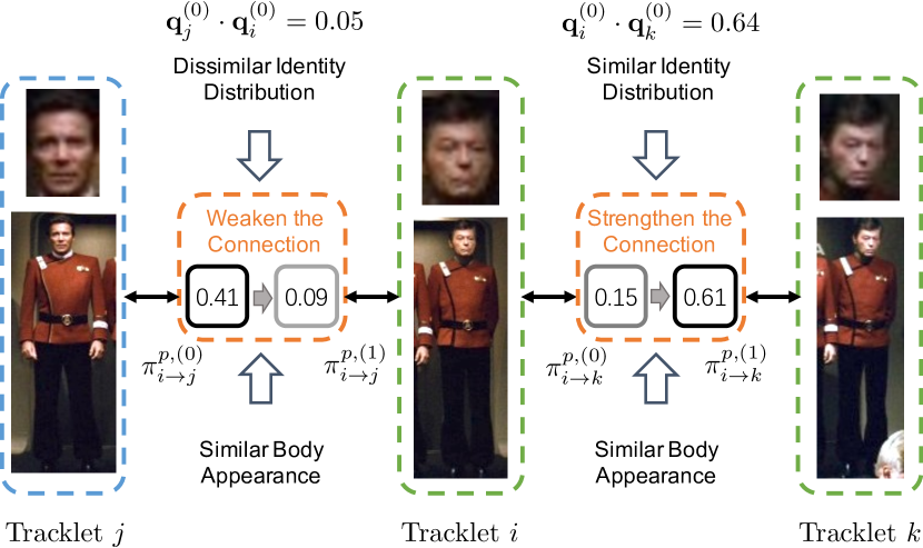
Figure 3: A qualitative example from the CSM dataset. The positive connection between tracklets $i$ and $j$ is initially strong because of the similar body appearance. During the inference step of the proposed method, this connection is weakened because of the divergent identity distributions between the two tracklets. It avoids erroneous information propagation through the connection. In contrast, the connection between tracklets $i$ and $k$ is strengthened due to their similar identity distributions.

Observations on IJB-S:

1. UGG vs FACE and PPCC [13]: UGG-U performs better than FACE and PPCC on almost all evaluation metrics with relatively large margin, in both protocols, which again shows the effectiveness of the proposed method.

2. UGG + Better Similarity Metric: UGG-U(sub) achieves state-of-the-art results by combining subspace-based similarity and UGG. It shows that the proposed method can further improve the performance over the improvement from the similarity metric.

3. EERR Metric: EERR metric [14] is relatively lower than identification accuracy, because it penalizes missed face detections, which is out of the scope of this paper.

Run time: From Table 4, we observe that UGG runs five times faster than PPCC on most of the protocols, which shows that UGG is more suitable for testing on large graphs during inference.

Qualitative Results: To illustrate the effectiveness of the proposed approach, a qualitative example is also shown in Figure 3. Tracklets $i$ and $j$ belong to different identities and tracklets $i$ and $k$ belong to the same identity. The initialized positive gate probability $\pi_{i\to j}^{p,(0)}=0.41$ is greater than $\pi_{i\to k}^{p,(0)}=0.15$. If the gate is fixed, information will be erroneously propagated between $i$ and $j$. Using the proposed method, we can adaptively update the gate based on the identity information from $i$ and $j$. Since identity distribution similarity $\mathbf{q}_{j}^{(0)}\cdot\mathbf{q}_{i}^{(0)}=0.05$ is very small, the two tracklets are unlikely to have the same identity. Hence the positive connection $\pi_{i\to j}^{p,(1)}=0.09$ is weakened after the update. Similarly, since $\mathbf{q}_{i}^{(0)}\cdot\mathbf{q}_{k}^{(0)}=0.64$ is large, the positive connection $\pi_{i\to k}^{p,(1)}=0.61$ is strengthened correspondingly.

Configurations				CSM in avg				CSM in max				IJB-S in favg
				IN		ACROSS		IN		ACROSS		S2SG		S2B
PG	PGcl	NG	aG	mAP	R@1	mAP	R@1	mAP	R@1	mAP	R@1	A@1	E@1	A@1	E@1
				58.72%	76.19%	55.67%	53.15%	61.29%	76.64%	58.20%	54.60%	64.86%	29.62%	66.48%	30.38%
✓				61.14%	84.95%	62.00%	66.02%	61.60%	84.79%	62.05%	64.63%	71.21%	30.66%	72.05%	31.37%
	✓			-	-	-	-	-	-	-	-	71.26%	30.73%	72.16%	31.54%
	✓	✓		-	-	-	-	-	-	-	-	73.24%	32.35%	73.78%	32.88%
✓			✓	62.81%	85.21%	63.30%	66.73%	63.74%	84.93%	63.42%	65.72%	72.32%	30.92%	73.15%	31.64%
	✓		✓	-	-	-	-	-	-	-	-	72.46%	31.02%	73.28%	31.73%
	✓	✓	✓	-	-	-	-	-	-	-	-	74.20%	32.70%	74.79%	33.29%

Table 5: Ablation study. In configurations, PG stands for adding positive gates for positive information. PGcl stands for adding positive gates with extra control from cannot-links. NG stands for adding negative gates for negative information. aG stands for adaptively updating positive gates. A@1 stands for Average Accuracy with filtering at R@1. E@1 stands for EERR without filtering at R@1.

Configurations			IN				ACROSS
PGTrain	aGTrain	UGGTest	mAP	R@1	R@3	R@5	mAP	R@1	R@3	R@5
			61.13%	77.86%	91.79%	96.65%	58.34%	56.56%	63.83%	66.34%
✓			61.39%	77.99%	91.77%	96.61%	58.94%	57.31%	64.26%	66.88%
✓	✓		61.40%	78.12%	91.85%	96.67%	58.70%	57.64%	64.49%	67.22%
		✓	64.14%	85.90%	95.42%	98.10%	65.82%	69.45%	76.83%	79.34%
✓		✓	64.58%	86.36%	95.53%	98.27%	66.90%	70.74%	77.83%	80.02%
✓	✓	✓	64.60%	86.68%	95.56%	98.24%	67.09%	71.31%	77.93%	80.39%

Table 6: Additional study on semi-supervised training on CSM dataset. PGTrain stands for using fixed positive gates during training. aGTrain stands for adaptively updating the gates during training. UGGTest stands for using UGG model during testing. In all experiments, only 25% of the training samples are labeled.

4.5 Ablation Studies

We conduct ablation studies on CSM and IJB-S datasets to show the effectiveness of key features in the proposed model. The results are shown in Table 5. We start from the baseline FACE without any information propagation, then gradually add key features of the method: PG: add fixed positive gates to propagate positive information. PGcl: same as PG except that positive information will not be propagated when cannot-link exists. NG: add negative gates to propagate negative information. aG: adaptively update positive gates in PG or PGcl using the proposed method. Since detection information is not given in the CSM dataset, there is no co-occurrence cannot-links available and we do not use negative gates in this dataset. Thus, the proposed method UGG-U corresponds to PG+aG on the CSM dataset and PGcl+NG+aG on the IJB-S dataset.

From Table 5 we observe that: 1) by introducing fixed positive gates, the performance improves compared to the baseline results, which indicates that positive information propagation controlled by body similarity improves the performance. 2) by adding cannot-links to control the positive gates as well, marginal improvements are obtained. Thus, the performance improvement is limited if allow only positive information to propagate. 3) by introducing additional negative gates using the same cannot-links, the performance improves significantly, which demonstrates the effectiveness of allowing negative information to propagate between tracklets. 4) finally, by adaptively updating the positive gates, we achieve the best performance in all protocols of both datasets. The result implies the advantages of adaptively updated gates.

4.6 Experiments on Different Training Settings

We also perform additional experiments on semi-supervised training on the CSM dataset with results shown in Table 6. In the experiment, similar to the UGG-ST setting, we first randomly pick 25% tracklets in each graph as labeled samples, and the rest 75% as unlabeled. We only train the linear embedding on face features with fixed UGG module on these training data.

Suppose after applying the embedding we want to learn, the similarities between galleries and labeled/unlabeled tracklets are $\mathbf{S}^{gt}=\begin{bmatrix}\mathbf{S}^{gt}_{l},\mathbf{S}^{gt}_{u}\end{bmatrix}$. We use three different settings to train the embedding: 1) directly train on the labeled similarities $\mathbf{S}^{gt}_{l}$ using cross-entropy loss, without invoking the UGG module. 2) use the UGG module with positive gates to process $\mathbf{S}^{gt}$ and train on the output similarity $\tilde{\mathbf{S}}^{gt}_{l}$ corresponding to the labeled tracklets by cross-entropy loss, denoted as PGTrain. 3) adaptively update the positive gates used in PGTrain, denoted as aGTrain. Please refer to the Supplementary Material for training details.

Two settings are used to test the performance of the embedding: 1) directly test on $\mathbf{S}^{gt}$ from the learned embedding, without using the UGG as post-processing. 2) test on $\tilde{\mathbf{S}}^{gt}$ from the learned embedding and with the UGG post-processing, denoted as UGGTest.

From the results in Table 6, we observe that in the semi-supervised setting, the embedding trained with the UGG is more discriminative than the one trained without the module. It achieves better performance in both test settings. It shows that by propagating information between tracklets, the UGG also leverages the information from those unlabeled tracklets during training, which is important for semi-supervised learning. Also, the UGG with adaptive gates performs better than fixed gates, which demonstrates that adaptive gates is also helpful during training by propagating the information more precisely between tracklets.

5 Conclusions and Future Work

In this paper, we proposed a graphical model-based method for video-based face recognition. The method propagates positive and negative identity information between tracklets through adaptive connections, which are influenced by both contextual information and identity distributions between tracklets. The proposed method can be either used for post-processing, or trained in supervised and semi-supervised fashions. It achieves state-of-the-art results on CSM and IJB-S datasets. An interesting future work will be using attribute information, such as gender, to construct negative connections and adaptively update negative gates.

References

- [1] Jun-Cheng Chen, Vishal M. Patel, and Rama Chellappa. Unconstrained face verification using deep CNN features. In WACV, March 2016.
- [2] Jun-Cheng Chen, Rajeev Ranjan, Swami Sankaranarayanan, Amit Kumar, Ching-Hui Chen, Vishal M. Patel, Carlos D. Castillo, and Rama Chellappa. Unconstrained still/video-based face verification with deep convolutional neural networks. IJCV, 126(2):272–291, Apr 2018.
- [3] Liang-Chieh Chen, George Papandreou, Iasonas Kokkinos, Kevin Murphy, and Alan L. Yuille. Deeplab: Semantic image segmentation with deep convolutional nets, atrous convolution, and fully connected CRFs. TPAMI, 40(4):834–848, 2018.
- [4] Liang-Chieh Chen, George Papandreou, Iasonas Kokkinos, Kevin Murphy, and Alan Loddon Yuille. Semantic image segmentation with deep convolutional nets and fully connected crfs. CoRR, abs/1412.7062, 2015.
- [5] Jiankang Deng, Jia Guo, Xue Niannan, and Stefanos Zafeiriou. Arcface: Additive angular margin loss for deep face recognition. In CVPR, 2019.
- [6] Changxing Ding and Dacheng Tao. Trunk-branch ensemble convolutional neural networks for video-based face recognition. CoRR, abs/1607.05427, 2016.
- [7] Ming Du and Rama Chellappa. Face association across unconstrained video frames using conditional random fields. In Computer Vision – ECCV 2012, pages 167–180, Berlin, Heidelberg, 2012. Springer Berlin Heidelberg.
- [8] Sixue Gong, Yichun Shi, Anil K. Jain, and Nathan D. Kalka. Recurrent embedding aggregation network for video face recognition. CoRR, abs/1904.12019, 2019.
- [9] Sixue Gong, Yichun Shi, Nathan D. Kalka, and Anil K. Jain. Video face recognition: Component-wise feature aggregation network (C-FAN). CoRR, abs/1902.07327, 2019.
- [10] Mikael Henaff, Joan Bruna, and Yann LeCun. Deep convolutional networks on graph-structured data. CoRR, abs/1506.05163, 2015.
- [11] Hexiang Hu, Guang-Tong Zhou, Zhiwei Deng, Zicheng Liao, and Greg Mori. Learning structured inference neural networks with label relations. 2016 IEEE Conference on Computer Vision and Pattern Recognition (CVPR), pages 2960–2968, 2016.
- [12] Gary B. Huang, Manu Ramesh, Tamara Berg, and Erik Learned-Miller. Labeled faces in the wild: A database for studying face recognition in unconstrained environments. Technical report, University of Massachusetts, Amherst, 2007.
- [13] Qingqiu Huang, Wentao Liu, and Dahua Lin. Person search in videos with one portrait through visual and temporal links. In Vittorio Ferrari, Martial Hebert, Cristian Sminchisescu, and Yair Weiss, editors, Computer Vision – ECCV 2018, pages 437–454, Cham, 2018. Springer International Publishing.
- [14] Nathan D. Kalka, Brianna Maze, James A. Duncan, Kevin J. O’Connor, Stephen Elliott, Kaleb Hebert, Julia Bryan, and Anil K. Jain. IJB-S : IARPA Janus Surveillance Video Benchmark. 2018.
- [15] Philipp Krähenbühl and Vladlen Koltun. Efficient inference in fully connected crfs with gaussian edge potentials. In J. Shawe-Taylor, R. S. Zemel, P. L. Bartlett, F. Pereira, and K. Q. Weinberger, editors, Advances in Neural Information Processing Systems 24, pages 109–117. Curran Associates, Inc., 2011.
- [16] Vijay Kumar, Anoop M. Namboodiri, and C. V. Jawahar. Face recognition in videos by label propagation. In 2014 22nd International Conference on Pattern Recognition, pages 303–308, Aug 2014.
- [17] John D. Lafferty, Andrew McCallum, and Fernando C. N. Pereira. Conditional random fields: Probabilistic models for segmenting and labeling sequence data. In Proceedings of the Eighteenth International Conference on Machine Learning, ICML ’01, pages 282–289, San Francisco, CA, USA, 2001. Morgan Kaufmann Publishers Inc.
- [18] Chung-Wei Lee, Wei Fang, Chih-Kuan Yeh, and Yu-Chiang Frank Wang. Multi-label zero-shot learning with structured knowledge graphs. 2018 IEEE/CVF Conference on Computer Vision and Pattern Recognition, pages 1576–1585, 2018.
- [19] Brianna Maze, Jocelyn Adams, James A. Duncan, Nathan Kalka, Tim Miller, Charles Otto, Anil K. Jain, W. Tyler Niggel, Janet Anderson, Jordan Cheney, and Patrick Grother. IARPA Janus Benchmark - C: Face dataset and protocol. In 2018 International Conference on Biometrics (ICB), pages 158–165, Feb 2018.
- [20] Omkar M. Parkhi, Andrea Vedaldi, and Andrew Zisserman. Deep face recognition. In BMVC, 2015.
- [21] Rajeev Ranjan, Ankan Bansal, Hongyu Xu, Swami Sankaranarayanan, Jun-Cheng Chen, Carlos D. Castillo, and Rama Chellappa. Crystal loss and quality pooling for unconstrained face verification and recognition. CoRR, abs/1804.01159, 2018.
- [22] Franco Scarselli, Marco Gori, Ah Chung Tsoi, Markus Hagenbuchner, and Gabriele Monfardini. The graph neural network model. IEEE Transactions on Neural Networks, 20(1):61–80, Jan 2009.
- [23] Florian Schroff, Dmitry Kalenichenko, and James Philbin. Facenet: A unified embedding for face recognition and clustering. In CVPR, June 2015.
- [24] Rasha Sheikh, Martin Garbade, and Juergen Gall. Real-time semantic segmentation with label propagation. In ECCV Workshops, 2016.
- [25] Yantao Shen, Hongsheng Li, Shuai Yi, Dapeng Chen, and Xiaogang Wang. Person re-identification with deep similarity-guided graph neural network. In ECCV, 2018.
- [26] Yi Sun, Yuheng Chen, Xiaogang Wang, and Xiaoou Tang. Deep learning face representation by joint identification-verification. In NIPS. 2014.
- [27] Yi Sun, Xiaogang Wang, and Xiaoou Tang. Deeply learned face representations are sparse, selective, and robust. In CVPR, June 2015.
- [28] Yaniv Taigman, Ming Yang, Marc’Aurelio Ranzato, and Lior Wolf. Deepface: Closing the gap to human-level performance in face verification. In CVPR, 2014.
- [29] Subarna Tripathi, Serge J. Belongie, Youngbae Hwang, and Truong Q. Nguyen. Detecting temporally consistent objects in videos through object class label propagation. 2016 IEEE Winter Conference on Applications of Computer Vision (WACV), pages 1–9, 2016.
- [30] Xiaolong Wang, Yufei Ye, and Abhinav Gupta. Zero-shot recognition via semantic embeddings and knowledge graphs. CVPR, 2018.
- [31] Cameron Whitelam, Emma Taborsky, Austin Blanton, Brianna Maze, Jocelyn Adams, Tim Miller, Nathan Kalka, Anil K. Jain, James A. Duncan, Kristen Allen, Jordan Cheney, and Patrick Grother. IARPA Janus Benchmark-B face dataset. CVPRW, 2017.
- [32] Lior Wolf, Tal Hassner, and Itay Maoz. Face recognition in unconstrained videos with matched background similarity. CVPR, pages 529–534, 2011.
- [33] Jingxiao Zheng, Rajeev Ranjan, Ching-Hui Chen, Jun-Cheng Chen, Carlos D. Castillo, and Rama Chellappa. An automatic system for unconstrained video-based face recognition. CoRR, abs/1812.04058, 2018.
- [34] Shuai Zheng, Sadeep Jayasumana, Bernardino Romera-Paredes, Vibhav Vineet, Zhizhong Su, Dalong Du, Chang Huang, and Philip Torr. Conditional random fields as recurrent neural networks. In International Conference on Computer Vision (ICCV), 2015.
- [35] Xiaojin Zhu and Zoubin Ghahramani. Learning from labeled and unlabeled data with label propagation. Technical report, 2002.