Determination of the scalar and vector polarizabilities of the cesium $6s\ ^{2}S_{1/2}\rightarrow 7s\ ^{2}S_{1/2}$ transition and implications for atomic parity non-conservation

Abstract

Using recent high-precision measurements of electric dipole matrix elements of atomic cesium, we make an improved determination of the scalar ($\alpha$) and vector ($\beta$) polarizabilities of the cesium $6s\ ^{2}S_{1/2}\rightarrow 7s\ ^{2}S_{1/2}$ transition calculated through a sum-over-states method. We report values of $\alpha=-268.82\ (30)\ a_{0}^{3}$ and $\beta=27.139\ (42)\ a_{0}^{3}$ with the highest precision to date. We find a discrepancy between our value of $\beta$ and the past preferred value, resulting in a significant shift in the value of the weak charge $Q_{w}$ of the cesium nucleus. Future work to resolve the differences in the polarizability will be critical for interpretation of parity non-conservation measurements in cesium, which have implications for physics beyond the Standard Model.

Precision measurements of weak optical interactions in atoms can provide a sensitive means of probing the weak force between nucleons and electrons at low momentum transfer Bouchiat, M. A. and Bouchiat, C. (1974, 1975). The extent to which atomic parity non-conservation (PNC) measurements agree with standard model predictions can provide constraints on conjectures of ‘beyond standard model’ physics, which are based on new additional interactions involving, for example, a massive $Z^{\prime}$ boson Porsev et al. (2009, 2010); Dzuba et al. (2012); Erler and Langacker (2000); Diener et al. (2012), a light boson Boehm and Fayet (2004); Bouchiat and Fayet (2005); Dzuba et al. (2017), or axion-like particles Stadnik et al. (2018), or searches of dark energy Roberts et al. (2014a, b); Stadnik and Flambaum (2014a, b). Recent theoretical searches for dark matter Davoudiasl et al. (2012); Davoudiasl and Lewis (2014); Davoudiasl et al. (2014) are based on a hypothesized light dark boson that decays primarily to dark matter, but which also interacts weakly with standard model matter.

The most precise determination of the weak charge through atomic PNC measurements to date was carried out in atomic cesium. This determination is based on a precise measurement of the ratio $Im(\mathcal{E}_{\rm PNC})/\beta$ by Wood et al. Wood et al. (1997), where $Im(\mathcal{E}_{\rm PNC})$ is the electric dipole transition moment for the $6s\ ^{2}S_{1/2}\rightarrow 7s\ ^{2}S_{1/2}$ transition induced by the weak force interaction, and $\beta$ is the vector polarizability for the transition. The weak charge $Q_{w}$ is determined then as the product of $Im(\mathcal{E}_{\rm PNC})/\beta$, the polarizability $\beta$, and a proportionality factor $k_{PNC}\equiv Q_{w}/Im(\mathcal{E}_{\rm PNC})$, which must be determined through difficult atomic structure calculations Dzuba et al. (1989); Blundell et al. (1991, 1992); Derevianko (2000); Dzuba et al. (2001); Johnson et al. (2001); Kozlov et al. (2001); Dzuba et al. (2002); Flambaum and Ginges (2005); Porsev et al. (2009, 2010); Dzuba et al. (2012); Roberts et al. (2013). A new determination of $Im(\mathcal{E}_{\rm PNC})/\beta$ is currently under development in our laboratory, and Derevianko has announced plans to undertake a new calculation of $k_{PNC}$ Wieman and Derevianko (2019). In this paper, we report a new determination of the vector polarizability $\beta$, which is of higher precision than, but differs from, the previously accepted value Dzuba and Flambaum (2000); Bennett and Wieman (1999).

Since 2000, the most precise determination of $\beta$ has been based upon a theoretical value for the hyperfine-changing magnetic dipole matrix element $M1_{\rm hf}$ Dzuba and Flambaum (2000), and a laboratory determination of the ratio $M1_{\rm hf}/\beta$ Bennett and Wieman (1999). With a precision of 0.19%, this value of $\beta$ has been preferred over the value determined from a calculation of the scalar polarizability $\alpha$ using a sum-over-states approach Blundell et al. (1992); Safronova et al. (1999); Vasilyev et al. (2002); Dzuba et al. (2002), combined with a measurement of the ratio $\alpha/\beta$ Cho et al. (1997). The latter method requires precise measurements or theoretical values for the reduced electric dipole (E1) matrix elements $\langle np_{J}||r||ms_{1/2}\rangle$ with $m=6$ or $7$, $n\geq 6$ and $J=1/2$ or $3/2$. Many of these matrix elements were measured to great precision in the past thirty years Bouchiat, M.A. et al. (1984); Tanner et al. (1992); Young et al. (1994); Rafac and Tanner (1998); Rafac et al. (1999); Bennett et al. (1999); Vasilyev et al. (2002); Derevianko and Porsev (2002); Amini and Gould (2003); Bouloufa et al. (2007); Sell et al. (2011); Zhang et al. (2013); Antypas and Elliott (2013); Borvák (2014); Patterson et al. (2015); Gregoire et al. (2015), and in the last 3 years, our group has undertaken and completed high-precion measurements of the remainder of these eight matrix elements  Toh et al. (2018, 2019); Damitz et al. (tted).

We first present a new determination of $\alpha$ through a sum-over-states method Blundell et al. (1992); Vasilyev et al. (2002)

$$\alpha = \frac{1}{6}\sum_{n}\Bigg{[}\langle 7s_{1/2}||r||np_{1/2}\rangle\langle np_{1/2}||r||6s_{1/2}\rangle$$ (1)

$$\hskip 14.45377pt\times\left(\frac{1}{E_{7s}-E_{np_{1/2}}}+\frac{1}{E_{6s}-E_{np_{1/2}}}\right)$$

$$-\langle 7s_{1/2}||r||np_{3/2}\rangle\langle np_{3/2}||r||6s_{1/2}\rangle$$

$$\hskip 14.45377pt\times\left(\frac{1}{E_{7s}-E_{np_{3/2}}}+\frac{1}{E_{6s}-E_{np_{3/2}}}\right)\Bigg{]}$$

where $\langle np_{J}||r||ms_{1/2}\rangle$ are the E1 transition matrix elements, $E_{ms}$ and $E_{np_{J}}$ are state energies, and $J=1/2$ or $3/2$ is the electronic angular momentum of the state.

Table 1: E1 dipole matrix elements, eigenstate energies, and contributions to the scalar polarizability $\alpha$. This table shows our sum-over-states calculation, as given in Eq. (1), of the scalar polarizability $\alpha$. E1 elements for $n=6$ and $7$, are experimental values, as discussed in the text. ^aRefs. Toh et al. (2018, 2019), ^bRefs. Young et al. (1994); Rafac and Tanner (1998); Rafac et al. (1999); Derevianko and Porsev (2002); Amini and Gould (2003); Bouloufa et al. (2007); Zhang et al. (2013); Patterson et al. (2015); Gregoire et al. (2015); Tanner et al. (1992); Sell et al. (2011), ^cRef. Bennett et al. (1999) and this work, ^dRef. Damitz et al. (tted). Theory values of E1 elements ($8\leq n\leq 12$) are from Ref. Safronova et al. (2016) including the Supplemental Information. State energies are found in NIST tables Kramida et al. (2019).

$n$	$d\ (a_{0})$	$\delta d$(%)	$\delta\alpha\ (a_{0}^{3})$	$d\ (a_{0})$	$\delta d$(%)	$\delta\alpha\ (a_{0}^{3})$	$E_{np_{1/2}}$ (cm${}^{-1})$	$\alpha\ (a_{0}^{3})$	$\delta\alpha\ (a_{0}^{3})$
	$\langle 7s_{1/2}||r||np_{1/2}\rangle$			$\langle np_{1/2}||r||6s_{1/2}\rangle$
$6$	$-4.249^{a}$	$0.094$	$0.031$	$4.5057^{b}$	$0.035$	$0.011$	$11178.27$	$-32.54$	$0.03$
$7$	$10.325^{c}$	$0.05$	$0.019$	$0.2781^{d}$	$0.16$	$0.060$	$21765.35$	$-37.35$	$0.06$
$8$	$0.914$	$2.9$	$0.016$	$0.092$	$11$	$0.061$	$25708.84$	$-0.55$	$0.06$
$9$	$0.349$	$2.9$	$0.002$	$0.043$	$16$	$0.013$	$27637.00$	$-0.08$	$0.01$
$10$	$0.191$	$3.1$	$0.001$	$0.025$	$20$	$0.005$	$28726.81$	$-0.02$	$0.00$
$11$	$0.125$	$3.5$	$0.000$	$0.016$	$27$	$0.002$	$29403.42$	$-0.01$	$0.00$
$12$	$0.09$	$3.9$	$0.000$	$0.012$	$28$	$0.001$	$29852.68$	$-0.00$	$0.00$
	$\langle 7s_{1/2}||r||np_{3/2}\rangle$			$\langle np_{3/2}||r||6s_{1/2}\rangle$
$6$	$-6.489^{a}$	$0.077$	$0.072$	$-6.3398^{b}$	$0.035$	$0.033$	$11732.31$	$-92.93$	$0.08$
$7$	$14.344^{c}$	$0.05$	$0.051$	$-0.5742^{d}$	$0.10$	$0.101$	$21946.39$	$-102.05$	$0.11$
$8$	$1.62$	$2.2$	$0.053$	$-0.232$	$6.2$	$0.151$	$25791.51$	$-2.43$	$0.16$
$9$	$0.68$	$2.1$	$0.010$	$-0.130$	$7.4$	$0.035$	$27681.68$	$-0.47$	$0.04$
$10$	$0.396$	$2.2$	$0.004$	$-0.086$	$8.3$	$0.014$	$28753.68$	$-0.17$	$0.01$
$11$	$0.270$	$2.4$	$0.002$	$-0.063$	$8.9$	$0.007$	$29420.82$	$-0.08$	$0.01$
$12$	$0.201$	$3.7$	$0.002$	$-0.049$	$9.5$	$0.004$	$29864.54$	$-0.04$	$0.00$
							$\alpha_{n>12}=$	$-0.30$	$0.15$
							$\alpha_{vc}=$	$+0.2$	$0.1$
							$\alpha=$	$-268.82$	$0.30$

We show the E1 matrix elements $\langle 7s_{1/2}||r||np_{J}\rangle$ and $\langle np_{J}||r||6s_{1/2}\rangle$, and state energies $E_{np_{J}}$ for states with principal quantum number $6\leq n\leq 12$ used for our sum-over-states calculation in Table 1. In earlier calculations of $\alpha$ Safronova et al. (1999); Vasilyev et al. (2002), the terms contributing the most to the $0.4\%$ uncertainty in $\alpha=269.7(11)~{}a_{0}^{3}$ were the $\langle 7s_{1/2}||r||6p_{J}\rangle$ and $\langle 7p_{J}||r||6s_{1/2}\rangle$ matrix elements whose uncertainties at that time were $0.5\%$ and $0.6\%$, respectively. (The numbers in brackets following the value denote the 1 $\sigma$ uncertainty in the least significant digits.) In the following paragraphs, we summarize the recent contributions towards these matrix elements, which enable us to calculate a more precise value for $\alpha$.

6s-6p

The values for the $\langle 6s_{1/2}||r||6p_{J}\rangle$ matrix elements have been measured precisely in a variety of experiments. These include fast-beam laser Tanner et al. (1992); Rafac et al. (1999), time-resolved fluorescence Young et al. (1994), ultra-fast pump-probe laser Patterson et al. (2015), photoassociation Derevianko and Porsev (2002); Bouloufa et al. (2007); Zhang et al. (2013), ground-state polarizability Amini and Gould (2003) and atom interferometry Gregoire et al. (2015). We take the weighted average of these measurements, to obtain a precision of $\sim 0.035\%$ for these matrix elements.

7s-6p

In 2017, we used an asynchronous gated detection technique with a single-photon detector to measure the lifetime of the $7s$ state to a precision of $0.14\%$ Toh et al. (2018). We combine this high precision lifetime measurement with a measurement of the ratio of dipole matrix elements $\langle 7s_{1/2}||r||6p_{3/2}\rangle/\langle 7s_{1/2}||r||6p_{1/2}\rangle$ Toh et al. (2019) in order to determine the individual matrix elements to a precision of $<0.1\%$. This ratio measurement was based upon measurements of the influence of laser polarization on the two-photon $6s\rightarrow 7s$ transition rate.

7s-7p

We derive new values for the $7s-7p$ matrix elements from a dc Stark shift $\Delta\alpha_{6s7s}$ measurement of the $6s\rightarrow 7s$ transition Bennett et al. (1999), and our high precision determinations of the $7s-6p$ matrix elements. This is the same method as used in Ref. Safronova et al. (1999). The static polarizability $\alpha_{7s}$ depends primarily on the $7s-7p$ and $7s-6p$ values. We use $\Delta\alpha_{6s7s}$ Bennett et al. (1999) and high precision measurements of the ground state static polarizability $\alpha_{6s}$ Amini and Gould (2003); Gregoire et al. (2015) to calculate the static polarizability $\alpha_{7s}$ of the $7s$ state. We also use theoretical calculations of the ratio of $7s-7p_{J}$ matrix elements $R_{7s7p}=|\langle 7s_{1/2}||r||7p_{3/2}\rangle/\langle 7s_{1/2}||r||7p_{1/2}\rangle|=1.3892\>(3)$ Safronova et al. (1999) and for the $7s-np$ matrix elements where $n>7$ Safronova et al. (2016). The results of our determination are $\langle 7s_{1/2}||r||7p_{1/2}\rangle=10.325\>(5)~{}a_{0}$ and $\langle 7s_{1/2}||r||7p_{3/2}\rangle=14.344\>(7)~{}a_{0}$, an improvement in precision from $0.15\%$ in Safronova et al. (1999) to $0.05\%$ as presented here.

6s-7p

Most recently, we have completed a comprehensive study of the $6s\rightarrow 7p_{3/2}$ ($\lambda=456$ nm) and $6s\rightarrow 7p_{1/2}$ ($\lambda=459$ nm) line absorption strengths to determine the transition matrix elements $\langle 6s_{1/2}||r||7p_{3/2}\rangle$ and $\langle 6s_{1/2}||r||7p_{1/2}\rangle$  Damitz et al. (tted). These comparative studies yield the ratios of matrix elements $\langle 6s_{1/2}||r||6p_{1/2}\rangle/\langle 6s_{1/2}||r||7p_{3/2}\rangle$ and $\langle 6s_{1/2}||r||7p_{3/2}\rangle/\langle 6s_{1/2}||r||7p_{1/2}\rangle$. Then by using the very precise value of $\langle 6s_{1/2}||r||6p_{1/2}\rangle$ Tanner et al. (1992); Rafac and Tanner (1998); Young et al. (1994); Patterson et al. (2015); Rafac et al. (1999); Derevianko and Porsev (2002); Bouloufa et al. (2007); Zhang et al. (2013); Amini and Gould (2003); Gregoire et al. (2015), we obtain a value of $\langle 6s_{1/2}||r||7p_{3/2}\rangle$ with 0.10% uncertainty, and of $\langle 6s_{1/2}||r||7p_{1/2}\rangle$ with 0.16% uncertainty.

In Fig. 1 we show a plot that illustrates the current state of theory and experiment for these eight matrix elements. (This plot is an updated version of a plot that first appeared as Fig. 2 of Porsev et al. (2009).) Specifically, this plot shows the experimental uncertainties and the discrepancies between theory and experiment for selected transition matrix elements. The error bars indicate the experimental uncertainties, while markers show the difference between experiment and three recent theoretical works, including: Refs. Safronova et al. (1999) ($\circ$), Dzuba et al. (2001, 2002) ($*$), and Porsev et al. (2010) ($\times$). (Deviation $>0$ indicates the theoretical value is greater than the experimental value.) We observe that there is good agreement between experiment and theory to the $\sim 0.2\%$ level for most of these terms. All of the matrix elements $\langle ns_{1/2}||r||mp_{J}\rangle$ for $n,m=6,7$ have now been measured to a precision of 0.16% or better, clearing the way for a new determination of $\alpha$, and serve as important benchmarks for future atomic theory calculations of $k_{PNC}$.

Figure 1: A graphical summary of the current status of the measured and calculated matrix elements $\langle np_{J}||r||ms_{1/2}\rangle$, where $m,n=6$ or 7, and $J=1/2$ and $3/2$ in atomic cesium. The error bars show the magnitudes of the uncertainty of the measurements. The data points show the deviation between the most recent calculations of the matrix elements and the measured value. (Deviation $>0$ indicates the theoretical value is greater than the experimental value.) The calculated values are from Refs. Safronova et al. (1999) ($\circ$), Dzuba et al. (2001, 2002) ($*$), and Porsev et al. (2010) ($\times$).

Table 1 shows a term-by-term computation of the scalar polarizability $\alpha$ following Eq. (1). In the second and fifth columns, we list values of the E1 matrix elements $d=\langle 7s_{1/2}||r||np_{J}\rangle$ and $\langle np_{J}||r||6s_{1/2}\rangle$, respectively, for principal quantum number $n$. For $n=6$ and 7, we have already discussed the values that we use. For $n=8-12$, we use theoretical values of these matrix elements from Ref. Safronova et al. (2016). The signs of these matrix elements are consistent with the sign convention described in Refs. Dzuba et al. (1997); Toh et al. (2019). In each case, the percentage uncertainty of the matrix element $\delta d$ is listed in columns 3 and 6. We show in column nine the contribution of these elements to the scalar polarizability, using the energy of $np_{J}$ states listed in the table Kramida et al. (2019), and $E_{7s}=18535.53$ cm^-1. We also show the uncertainties $\delta\alpha$ resulting from $\delta d$ in this table; $\delta\alpha$ due to the uncertainty in $\langle 7s_{1/2}||r||np_{J}\rangle$ in column four and $\langle np_{J}||r||6s_{1/2}\rangle$ in column seven, and the quadrature sum of these in the final column.

The final contributions to $\alpha$ are from $np_{J}$ states with $n>12$, and valence-core contributions $\alpha_{vc}$. We calculate the contributions from Hartree-Fock (HF) bound state wavefunctions with $n>12$ (bound and continuum) with the aid of a B-spline basis set. The HF value $\alpha_{n>12}=-0.45\ a_{0}^{3}$ is obtained by subtracting the sum for $n=1$ to $12$, in a term-by term HF calculation, from the sum over the entire spline basis. Noting that the HF values for the known contributions to $\alpha$ for $n=6$ to $12$ are typically $\sim$30% too high, we estimate $\alpha_{n>12}=-0.30\ (15)\ a_{0}^{3}$. For the valence-core contributions, we determine $\alpha_{vc}=+0.2\ (1)\ a_{0}^{3}$, in agreement with the value reported in Vasilyev et al. (2002); Safronova et al. (1999).

The final value for the scalar polarizability that we report, $\alpha=-268.82\>(30)\ a_{0}^{3}$ is the sum of all the contributions listed in column nine of the table. The uncertainty $\delta\alpha=0.30\ a_{0}^{3}$ is the quadrature sum of the uncertainties listed in the tenth column. Note that the primary uncertainties now come from the uncertainties of the E1 matrix elements $\langle 6s_{1/2}||r||8p_{3/2}\rangle$ and $\langle 6s_{1/2}||r||7p_{3/2}\rangle$, and the tail contributions $\alpha_{n>12}$. Our calculated value of $\alpha$ is in agreement with prior calculations of $\alpha$ using the same sum-over-states method Blundell et al. (1992); Safronova et al. (1999); Vasilyev et al. (2002), but the 0.11% precision of the current determination is a significant improvement.

Table 2: This table lists several determinations of $\beta$ since 1997, and we have bolded the two highest precision determinations. The previous value of $\beta$ with the best precision combines a measurement in 1999 by Bennett et al. of $M1_{hf}/\beta$ and the calculation in 2000 of $M1_{hf}$. The determinations labeled “Sum over states $(\alpha)$” combine a calculation of $\alpha$ and the high precision measurement of $\alpha/\beta$ Cho et al. (1997). In this table, we have also listed our direct calculation of $\beta$ through a sum-over-states method, which has a large uncertainty due to cancellation of terms.

Year	Authors	Remarks	$\beta\ (a_{0}^{3})$
2019	This work	Sum over states $\bm{(\alpha)}$	27.139 (42)
2002	Dzu02 Dzuba et al. (2002)	Sum over states $(\alpha)$	27.15 (11)
2002	Vas02 Vasilyev et al. (2002)	Sum over states $(\alpha)$	27.22 (11)
2000	Dzu00 Dzuba and Flambaum (2000)	$\bm{M1_{hf}}$ calculation	26.957 (51)
1999	Ben99 Bennett and Wieman (1999)	$M1_{hf}/\beta$ expt	27.024 (80)
1999	Saf99 Safronova et al. (1999)	Sum over states $(\alpha)$	27.11 (22)
1999	Saf99 Safronova et al. (1999)	Sum over states $(\beta)$	27.16
1997	Dzu97 Dzuba et al. (1997)	Sum over states $(\alpha)$	27.15 (13)
1992	Blu92 Blundell et al. (1992)	Sum over states $(\beta)$	27.0 (2)

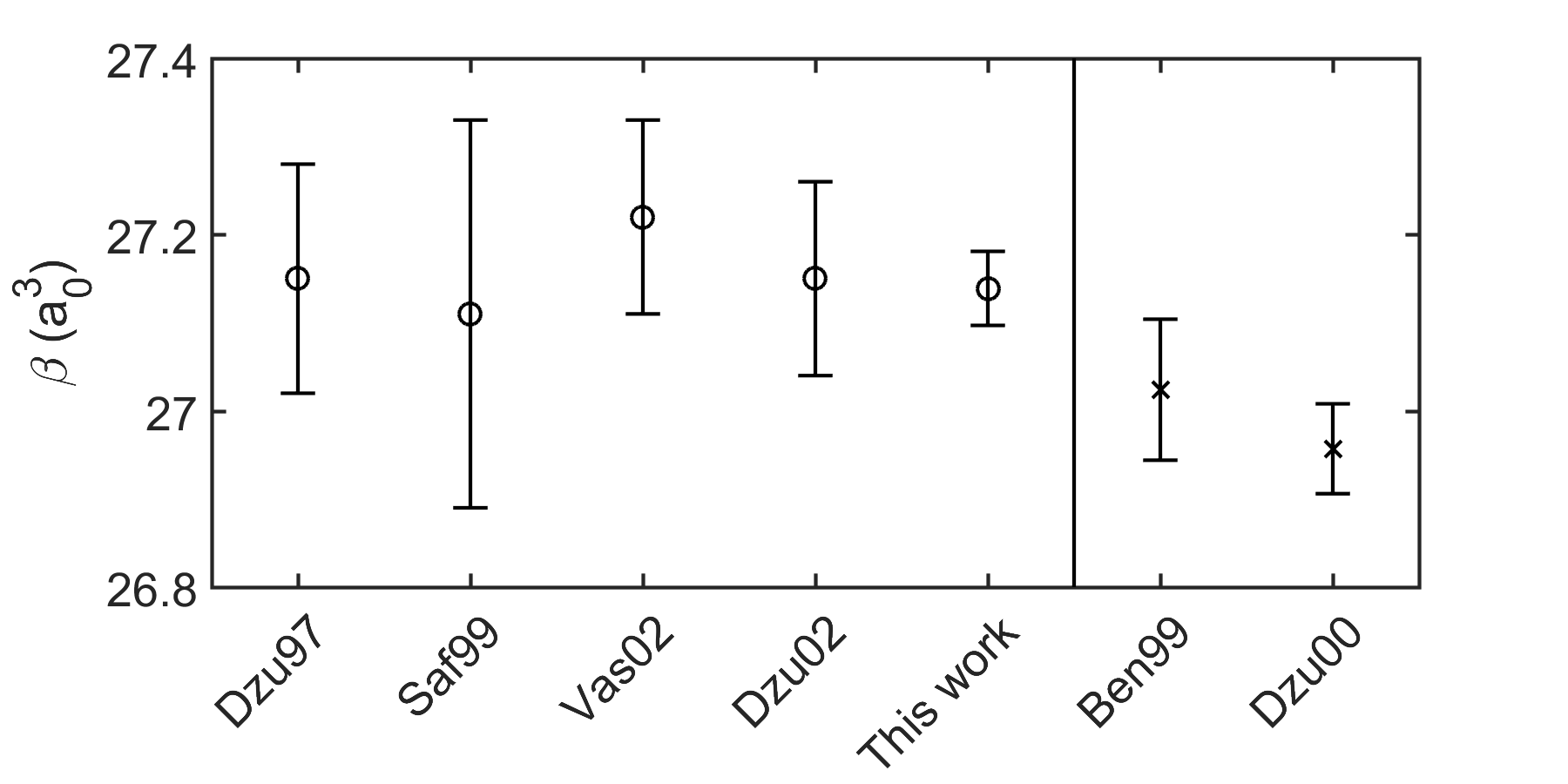
Figure 2: A summary of the current status of $\beta$ determinations. The $\beta$ values shown on the left (o) are determined through a sum-over-states of $\alpha$ and the ratio $\alpha/\beta$. The two values on the right (x) are determined through an experimental determination of $M1_{hf}/\beta$ and a theory value of $M1_{hf}$. Refer to Table 2 for references to these values.

From $\alpha$, we use the measured value of $\alpha/\beta=9.905\ (11)$ Cho et al. (1997) to derive

$$\beta=27.139\ (42)\ a_{0}^{3}.$$ (2)

We list this result, along with previous determinations of $\beta$ in Table 2, and show these data graphically in Fig. 2. The previous best determination of $\beta$, shown in bold font in Table 2, comes from a calculation of the hyperfine changing contribution to the magnetic dipole matrix element $M1_{hf}=0.8074(8)\times 10^{-5}~{}\mu_{B}/c$ Dzuba and Flambaum (2000), thought to be accurate to $0.1\%$, and the measurement of $M1_{hf}/\beta=-5.6195(91)$ V/cm Bennett and Wieman (1999). This results in $\beta=26.957\ (51)\ a_{0}^{3}$. These two results differ from one another by $0.182\ a_{0}^{3}~{}(0.67\%)$, which is larger than the sum of their uncertainties $0.093\ a_{0}^{3}~{}(0.34\%)$. The uncertainty in the new value is slightly smaller than that of the previous best value. We have also calculated $\beta=27.01\ (23)\ a_{0}^{3}$ directly from the E1 data displayed in Table 1 using the sum-over-states expression in Eq. (40) of Ref. Blundell et al. (1992). This value is in agreement with Eq. (2), but with much larger uncertainty due to significant cancellations between terms.

The new determination of the vector polarizability has an important implication for $Im(\mathcal{E}_{\rm PNC})$. The best measurement of $Im(\mathcal{E}_{\rm PNC})$ to date is the measurement in 1997 of

$$\frac{Im(\mathcal{E}_{\rm PNC})}{\beta}=1.5935(56)~{}\mathrm{mV/cm}$$ (3)

by Wood et al. Wood et al. (1997). (In the following, we base our analysis solely on this value, rather than the 2005 measurement of $Im(\mathcal{E}_{\rm PNC})/\beta=1.538(40)$ mV/cm by Guena et al. Guéna et al. (2005).)

To extract the weak charge $Q_{w}$ of the cesium nucleus from a measurement of $Im(\mathcal{E}_{\rm PNC})$, we need theoretical calculations of the proportionality $k_{PNC}$ between $Im(\mathcal{E}_{\rm PNC})$ and $Q_{w}$. Many-body calculations done by Porsev et al. (2009, 2010) determine

$$Im(\mathcal{E}_{\rm PNC})=0.8906(24)\times 10^{-11}|e|a_{0}\left(-Q_{w}/N\right).$$ (4)

The authors use the coupled-cluster method with full single, double and valence triple excitations considered. They also accounted for Breit, quantum electrodynamics (QED), and neutron skin corrections. The claimed $0.27\%$ uncertainty was obtained by comparison of calculations of energies, electric dipole amplitudes and hyperfine constants. Using Eq. (4) and our value of $\beta$ results in

$$Q_{w}=-73.66(28)_{e}(20)_{t}\ ,$$ (5)

where the experimental (e) and theoretical (t) uncertainties are indicated separately. This value of the weak charge is $\sim 1.2~{}\sigma$ larger than the standard model value Tanabashi et al. (2018)

$$Q_{SM}^{2018}=-73.23(1).$$ (6)

Dzuba et al. Dzuba et al. (2012); Roberts et al. (2013) introduced corrections to the core and tail contributions to $Im(\mathcal{E}_{\rm PNC})$ in Refs. Porsev et al. (2009, 2010) and determined

$$Im(\mathcal{E}_{\rm PNC})=0.8977(40)\times 10^{-11}|e|a_{0}\left(-Q_{w}/N\right),$$ (7)

in disagreement with Eq. (4), but in excellent agreement with their earlier results Dzuba et al. (2002); Flambaum and Ginges (2005). Combining Eq. (7) with our value of $\beta$ results in the value of

$$Q_{w}=-73.07(28)_{e}(33)_{t},$$ (8)

$\sim 0.3~{}\sigma$ less than $Q^{2018}_{SM}$.

We show in Fig. 3 the various determinations of $Q_{w}$ since 2002 Vasilyev et al. (2002); Dzuba et al. (2002); Flambaum and Ginges (2005); Porsev et al. (2009, 2010); Dzuba et al. (2012). The datapoint labeled $Q_{SM}^{2018}$ and the two horizontal lines denote the Standard Model prediction and its uncertainty Tanabashi et al. (2018). We note plans to resolve the differences between Eqs. (4) and (7) through a unified calculation of all contributions (principal, tail, and core) to $Im(\mathcal{E}_{PNC})$ Wieman and Derevianko (2019).

Figure 3: A summary of the current status of $Q_{w}$ determinations. The two horizontal lines denote the Standard Model prediction $Q^{2018}_{SM}$ Tanabashi et al. (2018). Past determinations are Vas02 Vasilyev et al. (2002), Dzu02 Dzuba et al. (2002), Fla05 Flambaum and Ginges (2005), Por10 Porsev et al. (2010), Dzu12 Dzuba et al. (2012).

In conclusion, we report a new, high-precision determination of the scalar ($\alpha$) and vector ($\beta$) polarizabilities of the cesium $6s\rightarrow 7s$ transition. This was achieved using precise values of E1 matrix elements between the lowest energy levels of cesium, which we determined from a combination of measurements and calculations. From that, we report new values for the weak charge of the cesium nucleus $Q_{w}$. There are still unresolved differences between the two most recent values of the vector polarizability $\beta$, which call for new calculations and/or measurements to address this issue. We note that any further improvement to the determination of $\alpha$ will require high precision measurements of a few key E1 matrix elements identified above, or alternatively, a direct laboratory determination of $\alpha$. Furthermore, any improvement to the value of $\beta$ as determined through the method described here will require a new laboratory measurement of $\alpha/\beta$, since the uncertainty of the current value of this ratio is of magnitude comparable to that of $\alpha$.

This material is based upon work supported by the National Science Foundation under Grant Number PHY-1460899.

References

- Bouchiat, M. A. and Bouchiat, C. (1974) Bouchiat, M. A. and Bouchiat, C., J. Phys. France 35, 899 (1974).
- Bouchiat, M. A. and Bouchiat, C. (1975) Bouchiat, M. A. and Bouchiat, C., J. Phys. France 36, 493 (1975).
- Porsev et al. (2009) S. G. Porsev, K. Beloy, and A. Derevianko, Phys. Rev. Lett. 102, 181601 (2009).
- Porsev et al. (2010) S. G. Porsev, K. Beloy, and A. Derevianko, Phys. Rev. D 82, 036008 (2010).
- Dzuba et al. (2012) V. A. Dzuba, J. C. Berengut, V. V. Flambaum, and B. Roberts, Phys. Rev. Lett. 109, 203003 (2012).
- Erler and Langacker (2000) J. Erler and P. Langacker, Physical Review Letters 84, 212 (2000).
- Diener et al. (2012) R. Diener, S. Godfrey, and I. Turan, Phys. Rev. D 86, 115017 (2012).
- Boehm and Fayet (2004) C. Boehm and P. Fayet, Nuclear Physics B 683, 219 (2004).
- Bouchiat and Fayet (2005) C. Bouchiat and P. Fayet, Physics Letters B 608, 87 (2005).
- Dzuba et al. (2017) V. A. Dzuba, V. V. Flambaum, and Y. V. Stadnik, Phys. Rev. Lett. 119, 223201 (2017).
- Stadnik et al. (2018) Y. V. Stadnik, V. A. Dzuba, and V. V. Flambaum, Phys. Rev. Lett. 120, 013202 (2018).
- Roberts et al. (2014a) B. M. Roberts, Y. V. Stadnik, V. A. Dzuba, V. V. Flambaum, N. Leefer, and D. Budker, Phys. Rev. D 90, 096005 (2014a).
- Roberts et al. (2014b) B. M. Roberts, Y. V. Stadnik, V. A. Dzuba, V. V. Flambaum, N. Leefer, and D. Budker, Phys. Rev. Lett. 113, 081601 (2014b).
- Stadnik and Flambaum (2014a) Y. V. Stadnik and V. V. Flambaum, Phys. Rev. D 89, 043522 (2014a).
- Stadnik and Flambaum (2014b) Y. V. Stadnik and V. V. Flambaum, Modern Physics Letters A 29, 1440007 (2014b).
- Davoudiasl et al. (2012) H. Davoudiasl, H.-S. Lee, and W. J. Marciano, Phys. Rev. Lett. 109, 031802 (2012).
- Davoudiasl and Lewis (2014) H. Davoudiasl and I. M. Lewis, Phys. Rev. D 89, 055026 (2014).
- Davoudiasl et al. (2014) H. Davoudiasl, H.-S. Lee, and W. J. Marciano, Phys. Rev. D 89, 095006 (2014).
- Wood et al. (1997) C. S. Wood, S. C. Bennett, D. Cho, B. P. Masterson, J. L. Roberts, C. E. Tanner, and C. E. Wieman, Science 275, 1759 (1997).
- Dzuba et al. (1989) V. Dzuba, V. Flambaum, and O. Sushkov, Physics Letters A 141, 147 (1989).
- Blundell et al. (1991) S. A. Blundell, W. R. Johnson, and J. Sapirstein, Phys. Rev. A 43, 3407 (1991).
- Blundell et al. (1992) S. A. Blundell, J. Sapirstein, and W. R. Johnson, Phys. Rev. D 45, 1602 (1992).
- Derevianko (2000) A. Derevianko, Phys. Rev. Lett. 85, 1618 (2000).
- Dzuba et al. (2001) V. A. Dzuba, V. V. Flambaum, and J. S. M. Ginges, Phys. Rev. A 63, 062101 (2001).
- Johnson et al. (2001) W. R. Johnson, I. Bednyakov, and G. Soff, Phys. Rev. Lett. 87, 233001 (2001).
- Kozlov et al. (2001) M. G. Kozlov, S. G. Porsev, and I. I. Tupitsyn, Phys. Rev. Lett. 86, 3260 (2001).
- Dzuba et al. (2002) V. A. Dzuba, V. V. Flambaum, and J. S. M. Ginges, Phys. Rev. D 66, 076013 (2002).
- Flambaum and Ginges (2005) V. V. Flambaum and J. S. M. Ginges, Phys. Rev. A 72, 052115 (2005).
- Roberts et al. (2013) B. M. Roberts, V. A. Dzuba, and V. V. Flambaum, Phys. Rev. A 87, 054502 (2013).
- Wieman and Derevianko (2019) C. Wieman and A. Derevianko, (2019), arXiv:1904.00281 [physics.atom-ph] .
- Dzuba and Flambaum (2000) V. A. Dzuba and V. V. Flambaum, Phys. Rev. A 62, 052101 (2000).
- Bennett and Wieman (1999) S. C. Bennett and C. E. Wieman, Physical Review Letters 82, 2484 (1999).
- Safronova et al. (1999) M. S. Safronova, W. R. Johnson, and A. Derevianko, Phys. Rev. A 60, 4476 (1999).
- Vasilyev et al. (2002) A. A. Vasilyev, I. M. Savukov, M. S. Safronova, and H. G. Berry, Phys. Rev. A 66, 020101(R) (2002).
- Cho et al. (1997) D. Cho, C. S. Wood, S. C. Bennett, J. L. Roberts, and C. E. Wieman, Phys. Rev. A 55, 1007 (1997).
- Bouchiat, M.A. et al. (1984) Bouchiat, M.A., Guena, J., and Pottier, L., J. Physique Lett. 45, 523 (1984).
- Tanner et al. (1992) C. E. Tanner, A. E. Livingston, R. J. Rafac, F. G. Serpa, K. W. Kukla, H. G. Berry, L. Young, and C. A. Kurtz, Phys. Rev. Lett. 69, 2765 (1992).
- Young et al. (1994) L. Young, W. T. Hill, S. J. Sibener, S. D. Price, C. E. Tanner, C. E. Wieman, and S. R. Leone, Phys. Rev. A 50, 2174 (1994).
- Rafac and Tanner (1998) R. J. Rafac and C. E. Tanner, Phys. Rev. A 58, 1087 (1998).
- Rafac et al. (1999) R. J. Rafac, C. E. Tanner, A. E. Livingston, and H. G. Berry, Phys. Rev. A 60, 3648 (1999).
- Bennett et al. (1999) S. C. Bennett, J. L. Roberts, and C. E. Wieman, Phys. Rev. A 59, R16 (1999).
- Derevianko and Porsev (2002) A. Derevianko and S. G. Porsev, Phys. Rev. A 65, 053403 (2002).
- Amini and Gould (2003) J. M. Amini and H. Gould, Phys. Rev. Lett. 91, 153001 (2003).
- Bouloufa et al. (2007) N. Bouloufa, A. Crubellier, and O. Dulieu, Phys. Rev. A 75, 052501 (2007).
- Sell et al. (2011) J. F. Sell, B. M. Patterson, T. Ehrenreich, G. Brooke, J. Scoville, and R. J. Knize, Phys. Rev. A 84, 010501(R) (2011).
- Zhang et al. (2013) Y. Zhang, J. Ma, J. Wu, L. Wang, L. Xiao, and S. Jia, Phys. Rev. A 87, 030503(R) (2013).
- Antypas and Elliott (2013) D. Antypas and D. S. Elliott, Phys. Rev. A 88, 052516 (2013).
- Borvák (2014) L. Borvák, Direct laser absorption spectroscopy measurements of transition strengths in cesium, Ph.D. thesis, University of Notre Dame (2014).
- Patterson et al. (2015) B. M. Patterson, J. F. Sell, T. Ehrenreich, M. A. Gearba, G. M. Brooke, J. Scoville, and R. J. Knize, Phys. Rev. A 91, 012506 (2015).
- Gregoire et al. (2015) M. D. Gregoire, I. Hromada, W. F. Holmgren, R. Trubko, and A. D. Cronin, Phys. Rev. A 92, 052513 (2015).
- Toh et al. (2018) G. Toh, J. A. Jaramillo-Villegas, N. Glotzbach, J. Quirk, I. C. Stevenson, J. Choi, A. M. Weiner, and D. S. Elliott, Phys. Rev. A 97, 052507 (2018).
- Toh et al. (2019) G. Toh, A. Damitz, N. Glotzbach, J. Quirk, I. C. Stevenson, J. Choi, M. S. Safronova, and D. S. Elliott, Phys. Rev. A 99, 032504 (2019).
- Damitz et al. (tted) A. Damitz, G. Toh, E. Putney, C. E. Tanner, and D. S. Elliott, (submitted).
- Safronova et al. (2016) M. S. Safronova, U. I. Safronova, and C. W. Clark, Phys. Rev. A 94, 012505 (2016).
- Kramida et al. (2019) A. Kramida, Y. Ralchenko, J. Reader, and NIST ASD Team, NIST Atomic Spectra Database (version 5.6.1) (2019).
- Dzuba et al. (1997) V. A. Dzuba, V. V. Flambaum, and O. P. Sushkov, Phys. Rev. A 56, R4357 (1997).
- Guéna et al. (2005) J. Guéna, M. Lintz, and M. A. Bouchiat, Phys. Rev. A 71, 042108 (2005).
- Tanabashi et al. (2018) M. Tanabashi et al. (Particle Data Group), Phys. Rev. D 98, 030001 (2018).