$BVRI$ Photometry of the Classic Type II-P Supernova 2017eaw in NGC 6946: Day 3 to Day 594

Abstract

Broadband $BVRI$ light curves of SN 2017eaw in NGC 6946 reveal the classic elements of a Type II-P supernova. The observations were begun on 16 May 2017 (UT), approximately 1 day after the discovery was announced, and the photometric monitoring was carried out over a period of nearly 600 days. The light curves show a well-defined plateau and an exponential tail which curves slightly at later times. An approximation to the bolometric light curve is derived and used to estimate the amount of ⁵⁶Ni created in the explosion; from various approaches described in the literature, we obtain $M$(${}^{56}{\rm Ni}$) = 0.115_-0.022^+0.027$M_{\odot}$. We also estimate that 43% of the bolometric flux emitted during the plateau phase is actually produced by the ⁵⁶Ni chain. Other derived parameters support the idea that the progenitor was a red supergiant.

1 Introduction

Type II-P supernovae are believed to be massive stars which undergo violent core collapse at a point in their evolution when they are red supergiants. Typically recognized by the presence of Balmer emission lines, and showing a characteristic “plateau" (or extended period of nearly constant brightness - the “P" in Type II-P) in their light curves, Type II-P supernovae constitute about 50% of all core-collapse supernovae. The “standard model" of such supernovae is that of a massive star that gradually builds up an iron core whose mass at some point exceeds the Chandrasekhar limit, and collapses violently into a neutron star. The shock wave from core collapse propagates through a deep envelope of hydrogen that is carried into space, leaving the neutron star as the remnant. Although models have suggested that stars in the range 8-30$M_{\odot}$ are the likely progenitors of Type II-P supernovae, most of the real progenitors that have been identified, usually in Hubble Space Telescope images, are in the range 8-16M_⊙. For an excellent review of the properties of all known types of supernovae, see Branch and Wheeler (2017).

Supernova 2017eaw was reported by Wiggins (2017) and confirmed by Dong & Stanek (2017) as the 10th supernova discovered in the “Fireworks Galaxy" NGC 6946. Wiggins’ discovery image, obtained on 2017 May 14.2383 (UT), revealed a new star 153^′′ northwest of the center of the galaxy at a magnitude of 12.8. Wiggins also obtained an image on May 12 that revealed nothing at the position of the new star, which pins down the explosion date to May 13$\pm$1 (UT), or JD 2457886.5 (see also Rui et al. 2019; Szalai et al. 2019; Van Dyk et al. 2019). An optical spectrum obtained by Tomasella et al. (2017) on 2017 May 15.13095 showed a P-Cygni type H$\alpha$ profile, indicating the supernova to be of Type II.

On May 16.256, we began a long-term campaign to monitor the $BVRI$ light curves of SN 2017eaw with the University of Alabama 0.4m DFM Engineering Ritchey-Chretien reflector. The observatory is located on campus atop Gallalee Hall, a severely light-polluted site. Later observations were made with larger telescopes at remote observatories in Arizona and the Canary Islands.

NGC 6946, type SAB(rs)cd (de Vaucouleurs et al. 1991; Buta et al. 2007), is a prototypical late-type spiral with a large population of massive stars. The galaxy is nearly face-on but lies at a Galactic latitude of only 11.^o7, and hence suffers considerable foreground extinction. The high northern declination facilitated nearly continuous coverage of the light curves except for the month of February, when the supernova could not be observed at night for a few weeks.

Here we present the results of our monitoring of SN 2017eaw over a period of nearly 600 days. Tsvetkov et al. (2018) also present $UBVRI$ photometry of SN 2017eaw to 206 days, with which we find good agreement. Other photometric observations are presented by Szalai et al. (2019), Rui et al. (2019), and Van Dyk et al. (2019). The observations reveal the classic light and colour evolution curves of a typical Type II-P supernova. From our light curves we also derive several basic parameters - e.g., absolute magnitude at maximum brightness, slope of the post-plateau decline in brightness, mass of ⁵⁶Ni produced, explosion energy, and estimated progenitor radius - to evaluate how SN 2017eaw compares to other supernovae of the same type.

2 Observations

In addition to the UA 0.4m telescope, two telescopes operated by the Southeastern Association for Research in Astronomy (SARA) were used for the observations of SN 2017eaw: the SARA-KP 0.96-m telescope at Kitt Peak, Arizona, and the SARA-RM (formerly Jacobus Kapteyn) 1.0-m telescope at the Roque de los Muchachos on La Palma, the Canary Islands. The SARA facilities are described by Keel et al. (2017) and are used remotely. Table 1 summarizes the CCDs, pixel scales, and other characteristics of the instruments used and of the images obtained.

Table 1: Properties of instruments and images. Col. 1: CCD camera; col. 2: observatory (KP=Kitt Peak, Arizona, USA; RM=Roque de los Muchachos, La Palma, Spain; UA = University of Alabama, Tuscaloosa, USA); col. 3: scale in arcsec pix^-1; col. 4: field dimensions in arcminutes covered by CCD frames; cols. 5 and 6: CCD properties; cols. 7 and 8: mean and standard deviation of the full width at half maximum of the point spread function on images, in pixels; and col. 9: number of nights in the mean.

CCD	Telescope	Pixel	Image	Gain	Read noise	$<$FWHM$>$	Std. Dev.	Number
		scale	dimensions	($e^{-}$/ADU)	($e^{-}$)	(pix)	(pix)	nights
1	2	3	4	5	6	7	8	9
ARC	SARA-KP 0.96-m	0.′′44	15.′0$\times$15.′0	2.3	6.0	7.0	2.3	6
Andor Icon-L	SARA-RM 1.0-m	0.′′34	11.′6$\times$11.′6	1.0	6.3	4.6	1.3	13
SBIG STL-6303E	UA 0.4m	0.′′57	29.′2$\times$19.′5	2.3	13.5	7.0	1.3	44

The filters used at all three observatories were manufactured by Custom Scientific as the Johnson/Cousins/Bessell $UBVRI$ filter set. The transmission curves for these filters are shown at the URL www.customscientific.com/astronomy.html. The nominal photon-weighted effective wavelengths for a spectrum flat in $F_{\lambda}$ as calculated from these data are $B$: 438.4 nm; $V$: 561.0 nm; $R$: 648.5 nm; and $I$: 831.3 nm. Decays in the coatings on the filters used with the UA 0.4m telescope led to large, donut-shaped flat-field features that were of minimal consequence in the $B$, $R$, and $I$ filters but were especially severe in the $V$ filter used up until November 2017. Filter rotation would lead to small displacements along one axis of the CCD that led to poor flat-fielding. The problem was minimized by exposing the twilight flats in the direction of the galaxy and by taking the $V$-band twilight flats last and the $V$-band observations of NGC 6946 first. This $V$-band filter was replaced with another of the same detailed characteristics, but with no flat-fielding issues. The change had little impact on the $V$-band transformations. For example, for 33 nights prior to 1 November 2017, the coefficients $C_{V0}$, $C_{V1}$, and $C_{V2}$ in equation 2a (section 3) were found on average to be 19.027$\pm$0.063, $-$0.008$\pm$0.016, and $-$0.020$\pm$0.012, respectively. The same coefficients after 1 November 2017 were found on average to be 19.336$\pm$0.053, 0.010$\pm$0.025, and $-$0.061$\pm$0.020 for 11 nights. The main effect of the filter change was to substantially reduce the average rms deviation of the UA 0.4m $V$-band transformations by a factor of 2.4, from 0.031 mag to 0.013 mag.

A typical UA 0.4m observation consisted of several 6 minute exposures, usually with more exposures in $B$ due to lower sensitivity of the CCD at shorter wavelengths. Typical SARA-RM and SARA-KP observations involved 2 to 5 1-5 min exposures. The images were flat-fielded, registered, and combined using Image Reduction and Analysis Facility (IRAF) routines IMARITH, IMALIGN, and IMCOMBINE. Photometry was performed using IRAF routine PHOT.

3 Set-up of Local Standard stars

3.1 Calibrations

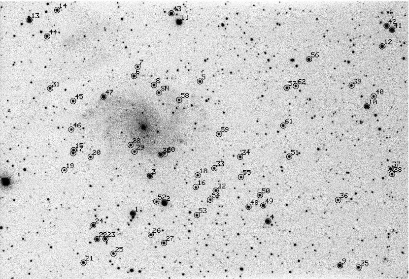
Figure 1: Local standards set up around NGC 6946. North is to the top and east is to the left. The supernova is labeled SN on this $I$-band UA 0.4m image.

The light curves for SN 2017eaw are based on the secondary local standards summarized in Table 3 and identified in Figure 1. These are based on averages from 5 photometric nights for $V$, $R$, and $I$, and 4 photometric nights for $B$. Standard stars from Landolt (1992) were used for estimating extinction and colour terms in the transformations of these stars to the Johnson-Cousins $BVRI$ system. The following transformation equations were used:

$$B=b-k_{B}x_{B}+C_{B0}+C_{B1}(B-V)+C_{B2}(B-V)^{2}$$

$$V=v-k_{V}x_{V}+C_{V0}+C_{V1}(B-V)+C_{V2}(B-V)^{2}$$

$$V=v-k_{V}x_{V}+C_{V0}+C_{V1}(V-R)+C_{V2}(V-R)^{2}$$

$$R=r-k_{R}x_{R}+C_{R0}+C_{R1}(V-R)+C_{R2}(V-R)^{2}$$

$$R=r-k_{R}x_{R}+C_{R0}+C_{R1}(R-I)+C_{R2}(R-I)^{2}$$

$$I=i-k_{I}x_{I}+C_{I0}+C_{I1}(R-I)+C_{I2}(R-I)^{2}$$

In these equations, $b$, $v$, $r$, and $i$ are the natural magnitudes outputted by IRAF routine PHOT and reduced to an integration time of 1 sec. For the UA 0.4m, these magnitudes were derived using an aperture of radius 15 pix with local sky readings taken in an annulus of inner radius 20 pix and a width of 10 pix. A growth curve showed that a 15 pix radius includes 98% of the total light of a point source on the UA 0.4m images. A similar aperture was used for the SARA-KP observations, but for the SARA-RM images obtained at later times we used an integration aperture radius of 6 pix to exclude a foreground star (section 3.2.2).

The $k$ coefficients in equations 1 are atmospheric extinction coefficients in units of magnitudes per unit airmass while the $x$ terms are the mean airmass for each filter at the midpoint of the time of observation. The $C$s are the zero points and colour terms. The latter are particularly important because not only does the galaxy suffer significant foreground extinction ($A_{V}$ $\approx$ 1 mag), but also the intrinsic colours of the supernova quickly reddened. This took the supernova into the domain of the reddest Landolt standards. The general procedure for applying equations 1-3 is to first solve for the colour index in each pair of equations, and then derive the individual magnitudes.

The graph in Figure 2 shows a standard magnitude + $kx$ (airmass term) versus standard colours. These highlight nonlinearities in the colour terms when the reddest stars have to be included. Table 2 summarizes mean values of the extinction and transformation coefficients for 4 nights for $VRI$ and 3 nights for $BV$ on the UA 0.4m telescope.

Table 2: Mean extinction and transformation coefficients for the UA 0.4m/STL-6303E combination for the nights of 23 November 2017UT, 11 December 2017UT, 12 December 2017UT, and 13 December 2017UT.

Filter	$k$	$C_{0}$	$C_{1}$	$C_{2}$	$n$	equation
	m.e.	m.e.	m.e.	m.e.
1	2	3	4	5	6	7
$B$	0.300	19.330	0.092	0.049	3	1a
	0.027	0.032	0.007	0.003
$V$	0.171	19.786	$-$0.025	0.000	3	1b
	0.019	0.019	0.004	0.000
$V$	0.180	19.793	$-$0.011	$-$0.018	4	2a
	0.015	0.015	0.027	0.021
$R$	0.110	19.978	$-$0.023	$-$0.119	4	2b
	0.015	0.027	0.020	0.013
$R$	0.118	19.995	$-$0.075	$-$0.046	4	3a
	0.013	0.018	0.006	0.003
$I$	0.069	19.235	0.011	0.031	4	3b
	0.011	0.011	0.013	0.002

Table 3: Local standard stars around NGC 6946. Col. 1: star number on $I$-band finding chart; cols. 2-5: magnitude and colours in the Johnson-Cousins $BVRI$ photometric system. The mean error (m.e.) of each parameter is on the line below the parameter

No.	$V$	$B-V$	$V-R$	$R-I$	No.	$V$	$B-V$	$V-R$	$R-I$	No.	$V$	$B-V$	$V-R$	$R-I$
	m.e.	m.e.	m.e.	m.e.		m.e.	m.e.	m.e.	m.e.		m.e.	m.e.	m.e.	m.e.
1	2	3	4	5	1	2	3	4	5	1	2	3	4	5
1	10.089	0.219	0.157	0.160	22	12.955	1.824	1.019	0.895	43	11.487	0.660	0.392	0.314
	0.009	0.009	0.014	0.011		0.010	0.045	0.010	0.011		0.011	0.007	0.013	0.017
2	10.432	1.447	0.784	0.667	23	12.676	1.252	0.711	0.636	44	12.666	0.753	0.481	0.405
	0.013	0.015	0.007	0.008		0.013	0.022	0.010	0.011		0.016	0.025	0.011	0.014
3	11.475	0.593	0.413	0.359	24	12.501	1.093	0.623	0.548	45	13.420	0.906	0.550	0.502
	0.017	0.007	0.017	0.012		0.012	0.021	0.011	0.012		0.013	0.017	0.021	0.016
4	11.775	1.540	0.869	0.742	25	13.341	0.577	0.368	0.346	46	13.795	0.659	0.412	0.381
	0.012	0.010	0.012	0.012		0.008	0.012	0.008	0.016		0.011	0.028	0.010	0.015
5	13.192	0.728	0.469	0.409	26	13.682	0.738	0.485	0.439	47	13.563	1.924	1.363	1.608
	0.012	0.015	0.012	0.016		0.018	0.026	0.017	0.018		0.019	0.039	0.016	0.015
6	13.117	1.172	0.677	0.615	27	13.231	0.950	0.585	0.460	48	12.491	0.525	0.347	0.315
	0.013	0.017	0.015	0.015		0.015	0.019	0.013	0.015		0.007	0.008	0.010	0.017
7	13.637	0.767	0.474	0.434	28	13.574	0.721	0.448	0.417	49	13.189	1.454	0.808	0.699
	0.019	0.008	0.019	0.013		0.015	0.028	0.010	0.019		0.011	0.018	0.011	0.015
8	13.272	0.633	0.441	0.381	29	13.774	0.671	0.456	0.411	50	13.646	1.158	0.794	0.596
	0.015	0.017	0.017	0.015		0.014	0.030	0.014	0.016		0.016	0.044	0.018	0.015
9	11.298	0.290	0.217	0.226	30	13.131	1.802	1.118	0.989	51	13.542	1.035	0.623	0.560
	0.009	0.013	0.010	0.014		0.013	0.054	0.012	0.011		0.013	0.024	0.015	0.014
10	12.653	1.967	1.164	1.238	31	12.960	0.632	0.443	0.387	52	14.000	0.616	0.421	0.388
	0.012	0.018	0.017	0.014		0.015	0.012	0.010	0.015		0.015	0.029	0.012	0.010
11	10.342	1.470	0.786	0.691	32	13.508	0.869	0.523	0.483	53	13.438	0.632	0.448	0.390
	0.013	0.010	0.011	0.012		0.016	0.024	0.012	0.012		0.019	0.009	0.016	0.013
12	11.823	0.487	0.354	0.309	33	13.488	0.562	0.386	0.342	54	13.909	0.723	0.426	0.395
	0.014	0.018	0.016	0.016		0.009	0.008	0.013	0.017		0.018	0.028	0.020	0.017
13	10.889	0.817	0.508	0.401	34	12.938	0.635	0.403	0.355	55	13.635	0.532	0.352	0.338
	0.022	0.017	0.022	0.013		0.009	0.012	0.010	0.015		0.011	0.007	0.010	0.016
14	12.277	0.435	0.323	0.293	35	12.653	0.640	0.411	0.358	56	12.763	0.948	0.609	0.557
	0.025	0.018	0.024	0.016		0.017	0.010	0.013	0.017		0.008	0.018	0.012	0.014
15	13.135	0.655	0.428	0.382	36	13.699	0.686	0.424	0.386	57	13.046	0.700	0.441	0.386
	0.011	0.012	0.009	0.015		0.019	0.016	0.020	0.015		0.012	0.019	0.014	0.016
16	13.804	0.738	0.464	0.442	37	12.893	1.220	0.800	0.694	58	14.124	0.659	0.406	0.405
	0.011	0.019	0.014	0.018		0.013	0.007	0.013	0.012		0.011	0.018	0.016	0.010
17	14.081	1.333	0.779	0.679	38	13.716	1.198	0.669	0.609	59	13.818	0.742	0.467	0.403
	0.013	0.038	0.024	0.016		0.020	0.037	0.022	0.014		0.020	0.019	0.021	0.014
18	14.366	1.254	0.699	0.618	39	13.700	1.236	0.706	0.620	60	14.826	0.949	0.587	0.456
	0.018	0.048	0.009	0.015		0.015	0.005	0.017	0.013		0.013	0.049	0.025	0.023
19	14.684	1.074	0.632	0.591	40	13.496	0.696	0.434	0.401	61	13.676	1.264	0.736	0.639
	0.025	0.047	0.036	0.018		0.016	0.024	0.014	0.016		0.014	0.030	0.016	0.016
20	14.262	1.367	0.716	0.665	41	10.938	0.657	0.435	0.383	62	13.688	0.527	0.390	0.357
	0.020	0.109	0.028	0.013		0.014	0.018	0.015	0.015		0.011	0.024	0.018	0.015
21	12.716	0.596	0.395	0.360	42	11.374	0.516	0.359	0.321	..	…..	…..	…..	…..
	0.017	0.012	0.016	0.014		0.013	0.012	0.016	0.015		…..	…..	…..	…..

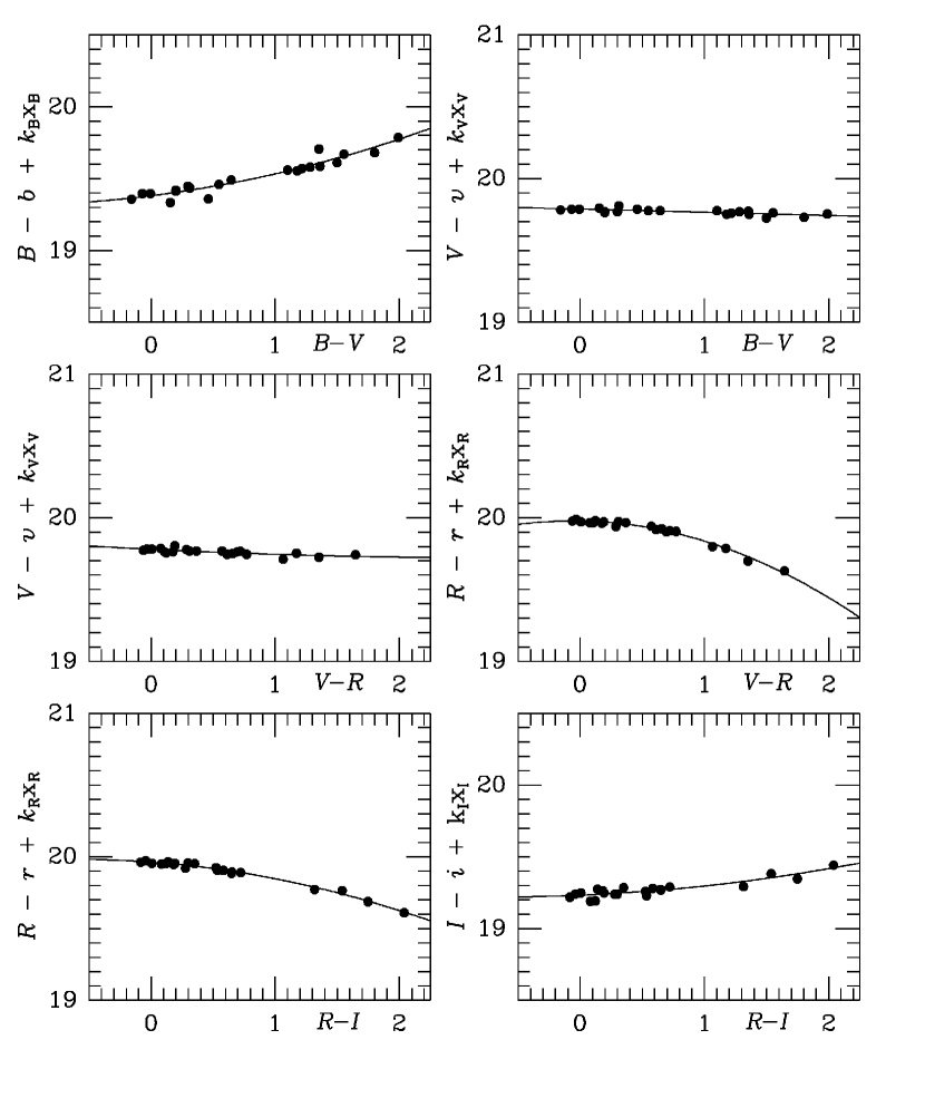
Figure 2: Graphs showing the nonlinear colour transformations derived from UA 0.4m observations of 15 Landolt (1992) standards on 11 December 2017 (UT).

The photometry in Table 3 was used exclusively to derive the magnitudes and colours of SN 2017eaw for the UA 0.4m observations. In these applications, it was neither necessary to know the airmass for any filter nor was it required that a given night be perfectly photometric. These local standards give similar results as the primary transformations shown in Figure 2, including a wide range of colour.

The Table 3 standards were also used for the SARA-RM and SARA-KP observations. However, many of these standards were saturated on the images and could not be used, including the reddest stars. In these cases, we supplemented the Table 3 standards with fainter local standards from Pozzo et al. (2006) and Botticella et al. (2009). In the Appendix a comparison is made between the magnitudes and colours from these and other sources with the system in Table 3. Only linear colour terms were used for the SARA observations, especially for the SARA-RM observations, most of which were made when the supernova was getting bluer.

3.2 Photometry

3.2.1 Transformation Issues

Standard stars like those of Landolt (1992) work well for establishing a set of local standards around any galaxy, but this does not mean they will work well for a supernova. The classification of any supernova as “Type II" is based on spectroscopy, in particular the presence of H$\alpha$ in emission. Prominent emission lines and other spectral features of supernovae can affect the reliability of the standard star transformations (e.g., Suntzeff et al. 1988; Stritzinger et al. 2002).

The transformation equations highlighted in the previous section give two estimates of the $R$-band magnitude: one from the $V-R$ calibration and one from the $R-I$ calibration. These equations also give two estimates for the $V$-band magnitude: one from the $B-V$ calibration and one from the $V-R$ calibration. We denote these estimates as $R1$ = $V-(V-R)$, $R2$ = $I+(R-I)$, $V1$ = $B-(B-V)$, and $V2$ = $R+(V-R)$.

For normal stars, $R1$ and $R2$ (and $V1$ and $V2$) should be the same to a few thousandths of a magnitude. The lower panel of Figure 3 shows that for SN 2017eaw, the difference $R1-R2$ is close to 0 for the first 100 days, then becomes negative a few tenths of a magnitude from about 100-300 days, and then becomes $\approx$0 again after 350 days. The use of the different symbols in Figure 3 shows that the effect is larger for the UA 0.4m observations compared to the SARA-KP and SARA-RM observations, especially at 250 days past explosion. This is likely due in part to our use of quadratic colour transformations for the UA 0.4m observations (Figure 2), compared to linear colour transformations for the SARA observations; some of the scatter may also be due to noise. A similar but lesser effect may be present in the $V$-band observations (upper panel of Figure 3), but could not be followed as thoroughly as in the $R$-band because the supernova became too faint to observe reliably in the $B$-band with the UA 0.4m by 130 days past explosion.

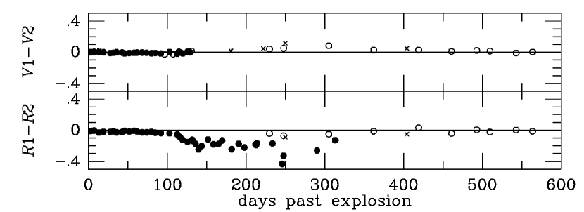
Figure 3: (top) The difference between $V1=B-(B-V)$ and $V2=R+(V-R)$ and (bottom) the difference between $R1=V-(V-R)$ and $R2=I+(R-I)$, both as a function of time after the explosion. The symbols are: UA 0.4m observations (filled circles), SARA-KP observations (crosses), and SARA-RM observations (open circles).

The significant $R1$ and $R2$ disagreements appear just after day 100, which corresponds approximately to the onset of the “nebular phase" in the supernova’s evolution. At this time, the spectrum of a Type II-P supernova (e. g., Leonard et al. 2002 and Silverman et al. 2017) begins to show prominent emission lines of H$\alpha$, [OI] 6300, 6364, [Ca II] 7291, 7324, and the near-infrared triplet Ca II 8498, 8542, and 8662. Szalai et al. (2019) show the spectral evolution of SN 2017eaw to 490 days past explosion, revealing that these lines did appear as expected with H$\alpha$ and the CaII near-infrared triplet being most prominent early-on and the [OI] and [CaII] 7291, 7324 lines appearing more strongly later.

In view of these effects we have adopted the following procedure for our light curves:

1. adopt $V$ from $V-R$

2. adopt $I$ from $R-I$

3. adopt $B$ from $V$ and $B-V$

4. adopt $R1$ from $V-R$ and $R2$ from $R-I$

5. derive $V-<R>$ and $<R>-I$ as colours, where $<R>$ is the average of $R1$ and $R2$. The average deviation between $R1$ and $R2$ is taken into account as part of the mean error of our $R$-band photometry.

Note that this procedure does not free our photometry from the effects of emission lines. Instead, it makes $V-R$, $R-I$ and $V-I$ more consistent. In general, the procedure on average reduced the values of $V-R$ from equations 2 by factors of 0.979 before the onset of the nebular phase, and 0.936 after onset, while the values of $R-I$ from equations 3 were reduced by factors of 0.963 before onset and 0.860 after onset. For a few observations where only $BVR$ or $RI$ photometry was obtained, the derived $V-R$ or $R-I$ colour index from equations 2 and 3 has been reduced slightly according to these factors, again for consistency.

3.2.2 Foreground Star

As SN 2017eaw faded, late-time ($>$ day 350) remote observations with the SARA-RM telescope revealed a foreground star lying 3.^′′4 to the northeast (Figure 4). From six measurements, the star has a magnitude and colours of $V$=19.90$\pm$0.04, $B-V$ = 1.04$\pm$0.04, $V-R$ = 0.63$\pm$0.03, and $R-I$ = 0.58$\pm$0.07. This star is close enough to the supernova that it would have been included in the integration apertures used for the earlier photometry. All observations prior to day 350 have been corrected for this star. The correction was made as $m_{c}=m_{*}-2.5log(x-1)$, where $m$ is the magnitude of the supernova from equations 1-3, $m_{*}$ is the magnitude of the foreground star in the same filter, and $x$=10${}^{-0.4(m-m_{*})}$. The correction generally amounted to $\leq$0.11 mag.

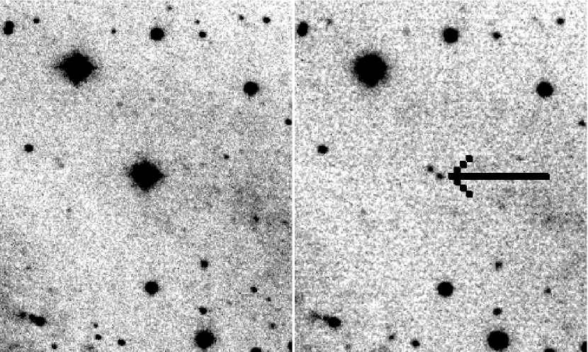
Figure 4: Comparison between SARA-RM $V$-band images of SN 2017eaw on (left) 17 August 2017 UT (day 97, $V$=13.5) and (right) 4 October 2018 UT (day 510, $V$ = 19.8), the latter revealing a foreground star ($V$ = 19.9) close to the SN. The field shown has dimensions 2.^′33 $\times$ 2.^′81. North is at the top and east is to the left. The supernova is indicated by the arrow.

4 Light Curves

4.1 Characteristics

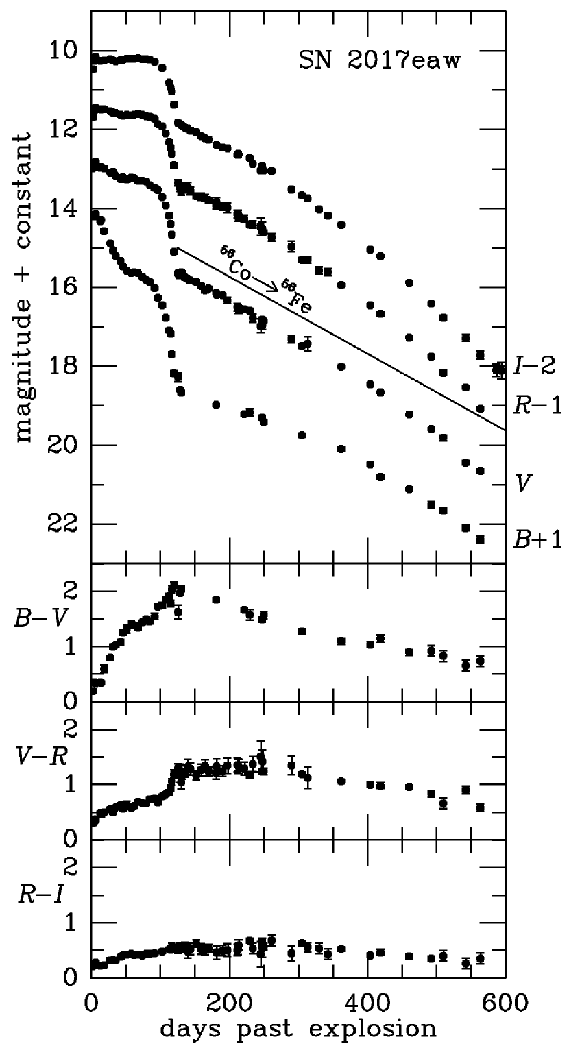
Figure 5: Light and color evolution curves of SN 2017eaw to 564 days past the explosion date for filters $B$, $V$, and $R$, and to 594 days for filter $I$. The line shows the decline rate expected for the decay of ⁵⁶Co to ⁵⁶Fe.

The resulting $BVRI$ photometry of SN 2017eaw is collected in Table 4 and the light and colour curves are shown in Figure 5. The light curves show all of the classic features of a Type II-P supernova (Arnett 1996): a point of peak brightness followed by a rapid decline in the $B$-band owing to cooling of the optically-thick, hot expanding gases; a plateau, most prominent in the $R$ and $I$-bands, owing to a drop in optical thickness as the gases cool, leading to the propogation of a mostly hydrogen recombination front through the expanding envelope; a sharp edge to the plateau, which occurs when the recombination front has passed through the entire envelope (supernebular phase); and finally, a sudden halt to the sharp decline of the plateau edge, owing to a new important light curve power source derived from a radioactive decay process, leading to a slow linear decline in magnitudes called the “tail." The plateau and the tail are the dominant features of the light curves of Type II-P supernovae, which represent about 40% of all supernovae and at least 50% of all core collapse supernovae (Smartt et al. 2009; see also Smartt 2009; Li et al. 2011).

The $B-V$ color evolution curve shows a fairly rapid rise from $B-V$$\approx$0.2 at 3 days past explosion to $B-V$$\approx$2.1 at 120 days past explosion. There is no sustained period at maximum redness in $B-V$; instead, the supernova reaches maximum $B-V$ for a few days, and then the color declines systematically but more slowly after the onset of the nebular phase. In contrast, both $V-R$ and $R-I$ show a sustained period of nearly constant color index lasting from about 120 days to at least 250 days past the explosion date.

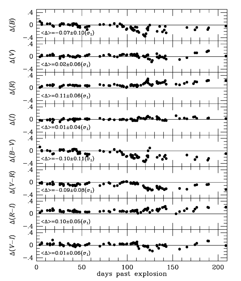
Figure 6: Comparison of Table 4 photometry of SN 2017eaw with that of Tsvetkov et al. (2018), for the first 200 days. The average and standard deviation of each difference is shown in the lower left of each frame.

Figure 6 compares our Table 4 photometry with the data of Tsvetkov et al. (2018), who presented $UBVRI$ observations of SN 2017eaw up to day 206. Our light curves are well-sampled during this interval, and in Figure 6 we compare our profiles with theirs by linearly interpolating their profiles to the dates of our observations. The differences are plotted as $\Delta$ = theirs (interpolated) $-$ ours, and show very good agreement for $V$, $I$, and $V-I$. For $B$ and $R$ there are small systematic disagreements that are likely attributable to transformation issues. Our $R$-band magnitudes on average differ from those of Tsvetkov et al. (2018) by 0.11$\pm$0.06 mag. This difference translates to comparable systematic differences in $V-R$ and $R-I$. In $B-V$, the curves are similar at early times, but by day 100 a systematic difference of a few tenths of a magnitude appears. The SN achieves a maximum $B-V$ in our dataset slightly redder than in the Tsvetkov et al. dataset. A similar comparison with the photometry of Szalai et al. (2019) gives $<\Delta$> = $-$0.05, $-$0.03, 0.06, and 0.06 mag, with standard deviations of 0.10, 0.06, 0.07, and 0.05 mag, for $B$, $V$, $R$, and $I$, respectively.

4.2 Distance, Reddening, and Extinction

The remainder of our analysis depends sensitively on the assumed distance to NGC 6946 and the total extinction affecting SN 2017eaw. Sahu et al. (2006) used a distance of 5.6 Mpc based on a variety of methods for their analysis of SN 2004et. Szalai et al. (2019) adopted a distance of 6.85$\pm$0.63 Mpc based on an average of distances estimated from the expanding photosphere method (EPM), the standard candle method (SCM), the tip of the red giant branch (TRGB) method, and the planetary nebula luminosity function (PNLF). However, Eldridge and Xiao (2019) have argued that the best distance estimate to use now for NGC 6946 is 7.72$\pm$0.32 Mpc, based on the TRGB method (Anand et al. 2018). This is the distance we adopt in this paper.

For the reddening, we adopted $E(B-V)$ = 0.41$\pm$0.05 mag based on the NaI D absorption line equivalent width detected towards SN 2004et (Zwitter et al. 2004). Using Table 3 of Cardelli et al. (1989), this translates to $A_{B}$ = 1.68, $A_{V}$ = 1.27, $A_{R}$= 1.06, and $A_{I}$ = 0.76 mag, which may be compared with the Galactic extinction values of $E(B-V)$ = 0.30, $A_{B}$ =1.241, $A_{V}$ = 0.938, $A_{R}$ = 0.742, and $A_{I}$ = 0.515 mag, given by the NASA/IPAC Extragalactic Database (NED) extinction calculator, based on the method of Schlafly and Finkbeiner (2011). Although there is considerable scatter in the correlation between NaI D equivalent width and $E(B-V)$ (Munari and Zwitter 1997), the extreme redness of both SN 2004et and SN 2017eaw favour the higher value of $E(B-V)$. This value was also adopted by Sahu et al. (2006) and Szalai et al. (2019), and also is within the uncertainty of the value of $E(B-V)$ = 0.59 $\pm$ 0.19 mag adopted by Rui et al. (2019).

4.3 Comparison with other SN II-P

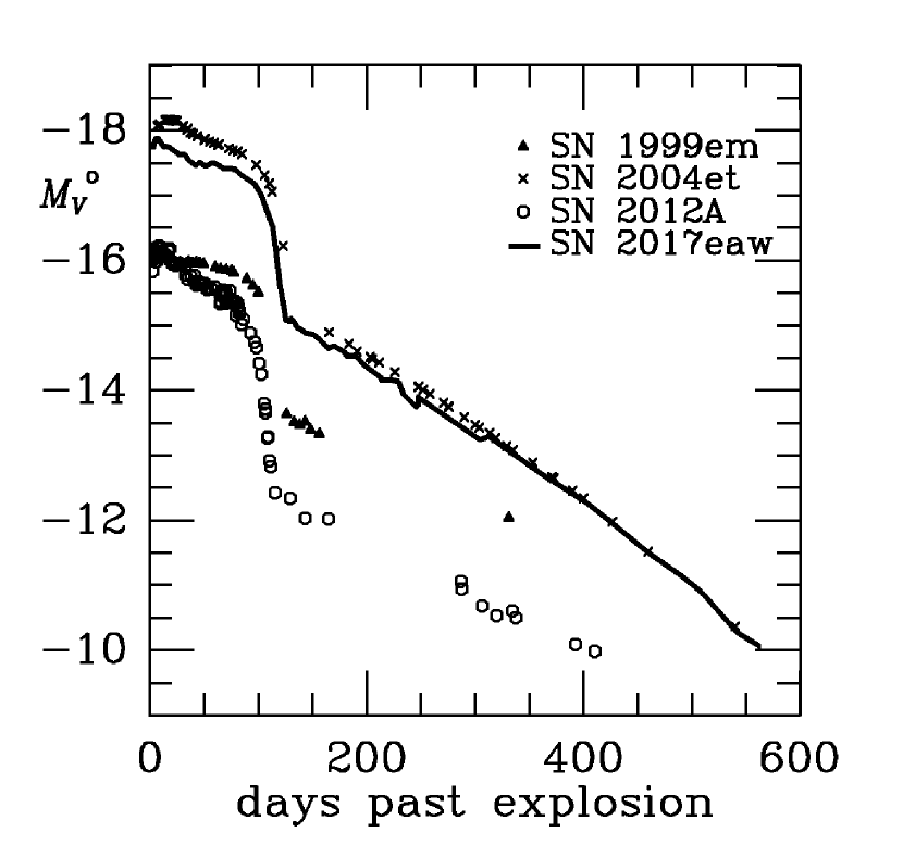
Figure 7: Comparison of extinction-corrected, absolute $V$-band light curves of SN 2017eaw with three other SN II-P. These assume a distance modulus of 29.44 for SN 2004et and 2017eaw (Anand et al. 2018), 29.57 for SN 1999em (Leonard et al. 2002), and 29.96 for SN 2012A (Tomasella et al. 2013).

Figure 7 compares the $V$-band light curves of SN 2017eaw with those of three other Type II-P supernovae: SN 1999em in NGC 1637 (Leonard et al. 2002), SN2004et in NGC 6946 (Sahu et al. 2006), and SN 2012A in NGC 3239 (Tomasella et al. 2013). The magnitude comparisons are in terms of absolute magnitudes $M_{V}^{o}$ using distance modulus/$E(B-V)$ values of 29.44/0.41 for SN 2004et and SN 2017eaw, 29.57/0.10 for NGC 1637 and 29.96/0.037 for SN 2012A. The results show that the tails of SN 2004et and SN 2017eaw are very similar in $V$-band brightness as well as shape. On the plateau, the two supernovae differ most significantly, by about 0.25 mag. In contrast, SN 1999em and SN 2012A appear to have been lower luminosity Type II supernovae by nearly 2 mag.

Figure 8 compares the color evolution of SN 2017eaw with the same three supernovae using reddening-corrected two-colour plots. The evolution of $(B-V)_{o}$ versus $(V-I)_{o}$ especially shows very similar curves for SN 2004et and SN 2017eaw, except that the former is displaced blueward by 0.1-0.2 mag in $(V-I)_{o}$, The points for SN 1999em and SN 2012A closely follow the curve for SN 2017eaw. Similar results are found for $(V-R)_{o}$ versus $(R-I)_{o}$

4.4 Derived Parameters

Tables 5– 8 summarize the derived parameters from the light curves. It appears the supernova was discovered already very close to maximum light. Although subtle, all four filters indicate that maximum light occurred on 2017 May 20 UT (JD 2457893.710), about 6 days after discovery. The apparent magnitudes at maximum light are corrected in Table 5 for the substantial foreground extinctions. The absolute magnitudes are close to $-$18.0 in all four filters. This is more luminous by about 2 mag than the average Type II SN (Li et al. 2011). Relative to maximum light, the brightness of the SN in the plateau phase ($B_{p}$, $V_{p}$, $R_{p}$, and $I_{p}$) is strongly dependent on passband, with $B_{p}-B$(max) = 1.5 mag compared to $I_{p}-I$(max) = 0.05 mag.

Past the plateau phase, the size of the dropoff relative to the plateau level is strongly wavelength dependent, ranging from $B_{r}-B_{p}$ = 2.84 mag to $I_{r}-I_{p}$ = 1.61 mag (Table 6). The tail begins at $\approx$125 days past explosion and continues to the end of the observing period, 469 days later. The light curves in this phase are generally interpreted as being powered by the decay of radioactive cobalt isotope ⁵⁶Co into stable iron isotope ⁵⁶Fe. The ⁵⁶Co is believed to have been produced by the decay of ⁵⁶Ni, the main isotope of iron group elements explosively produced by the post-core collapse shock wave running through the star (e.g., Jerkstrand 2011). The decay of ⁵⁶Ni into ⁵⁶Co is rapid, with a half-life of 6 days, while the decay of ⁵⁶Co into ⁵⁶Fe is 77 days (Nadyozhin 1994). If the gamma rays produced by the latter decay process are completely confined, then the light curves will show a linear decline at a rate of 0.98 mag (100 days)^-1 (line shown in Figure 5). Since this is generally observed, the slow, post plateau decline is often referred to as the “radioactive tail" of the light curves.

The properties of the tail seen in the light curves of SN 2017eaw support this idea. The results of linear least squares fits to the tail are summarized in Table 6, which lists the slopes $\gamma_{B}$, $\gamma_{V}$, $\gamma_{R}$, and $\gamma_{I}$ in units of magnitudes per 100 days. The decline is nearly linear in the $V$ band, but in $R$ and $I$ there appears to be a slight bend in the tail starting about 290 days past explosion. For this reason, Table 6 summarizes the parameters of the tail for two parts: the earlier part from 125-290 days after the explosion, and the later part from 290-564 days after the explosion. If the light curves past the plateau phase are due to a radioactive decay process, then (1.0857/slope)(ln2) gives an estimate of the half-life, $t_{1\over 2}$, of the process. The $B$-band slope is not well-determined in the earlier phase, but the $V$, $R$, and $I$ filters give values of $t_{1\over 2}$ ranging from 75.8 days to 82.2 days in this phase. These correspond to decline rates of $\gamma_{V}$ = 0.992 mag (100 days)^-1 and $\gamma_{I}$ = 0.924 mag (100 days)^-1, respectively. A combined $VRI$ fit using the mean early tail colours as offsets gives $t_{1\over 2}$ = 79.8$\pm$1.0 days, close to the nominal value for the decay of ⁵⁶Co to ⁵⁶Fe.

Past 290 days, the colours of the tail are generally bluer on average than the colours before 290 days. The decline rates also increase; e.g., $\gamma_{V}$ increases to 1.27 mag (100 days)^-1 while $\gamma_{I}$ increases to 1.56 mag (100 days)^-1. This change in decline rate could in part signify the breakdown of the gamma ray confinement assumption, at least at later times (Woosley et al. 1989; Sahu et al. 2006; Otsuka et al. 2012).

Table 4: Photometry of SN 2017eaw. Col. 1: Universal Time date; col. 2: number of days after explosion; cols. 3-6, line 1: magnitudes (corrected for foreground star) of SN 2017eaw; cols 3-6, line 2: errors on magnitudes; col. 7: telescope used

Date	Phase	$B$	$V$	$R$	$I$	Tel
(UT)	JD2457886.5+
1	2	3	4	5	6	7
05-16-2017	3.256	13.171	12.981	12.683	12.469	UA 0.4m
		0.024	0.024	0.017	0.024
05-18-2017	5.195	13.204	12.856	12.516	12.259	UA 0.4m
		0.025	0.023	0.022	0.024
05-20-2017	7.210	13.149	12.817	12.444	12.162	UA 0.4m
		0.031	0.026	0.014	0.021
05-26-2017	13.200	13.322	12.972	12.479	12.257	UA 0.4m
		0.020	0.015	0.017	0.015
05-27-2017	14.403	13.292	12.947	12.490	……	SARA-KP
		0.027	0.017	0.024	……
06-01-2017	19.162	13.575	12.980	12.480	12.252	UA 0.4m
		0.056	0.036	0.020	0.035
06-10-2017	28.123	13.888	13.091	12.534	12.217	UA 0.4m
		0.021	0.029	0.017	0.051
06-14-2017	32.105	14.068	13.074	12.571	12.245	UA 0.4m
		0.030	0.033	0.015	0.019
06-18-2017	36.074	14.201	13.172	12.587	12.269	UA 0.4m
		0.036	0.020	0.018	0.014
06-25-2017	43.102	14.331	13.252	12.628	12.241	UA 0.4m
		0.032	0.031	0.020	0.017
06-28-2017	46.106	14.466	13.209	12.645	12.238	UA 0.4m
		0.041	0.032	0.021	0.022
07-04-2017	52.110	14.578	13.265	12.631	12.207	UA 0.4m
		0.032	0.065	0.014	0.021
07-10-2017	58.221	14.634	13.216	12.640	12.202	UA 0.4m
		0.028	0.027	0.011	0.017
07-14-2017	62.090	14.617	13.232	12.621	12.207	UA 0.4m
		0.029	0.029	0.019	0.014
07-20-2017	68.098	14.636	13.295	12.607	12.188	UA 0.4m
		0.034	0.032	0.021	0.012
07-26-2017	74.123	14.733	13.295	12.625	12.214	UA 0.4m
		0.030	0.026	0.022	0.013
08-01-2017	80.103	14.816	13.317	12.658	12.219	UA 0.4m
		0.026	0.029	0.013	0.011
08-06-2017	85.103	14.855	13.403	12.667	12.230	UA 0.4m
		0.036	0.019	0.025	0.014
08-13-2017	92.089	15.016	13.474	12.726	12.278	UA 0.4m
		0.035	0.044	0.022	0.013
08-17-2017	96.939	15.258	13.536	12.858	……	SARA-RM
		0.042	0.020	0.024	……
08-24-2017	103.076	15.454	13.708	12.921	12.442	UA 0.4m
		0.040	0.029	0.025	0.012
08-28-2017	107.947	15.767	13.920	13.095	……	SARA-RM
		0.045	0.019	0.024	……
09-03-2017	113.069	16.092	14.185	13.325	12.808	UA 0.4m
		0.042	0.035	0.032	0.011
09-05-2017	115.089	16.172	14.392	13.450	12.938	UA 0.4m
		0.051	0.032	0.042	0.011
09-07-2017	117.094	16.694	14.660	13.612	13.036	UA 0.4m
		0.060	0.033	0.050	0.019
09-10-2017	120.082	17.178	15.093	13.903	13.364	UA 0.4m
		0.070	0.044	0.065	0.012
09-16-2017	126.098	17.273	15.646	14.353	13.826	UA 0.4m
		0.114	0.044	0.078	0.015
09-19-2017	129.113	17.590	15.625	14.469	……	UA 0.4m
		0.034	0.016	0.093	……
09-19-2017	129.205	……	15.677	14.428	13.870	SARA-KP
		……	0.091	0.077	0.016

Table 4: (cont.) Photometry of SN 2017eaw. Col. 1: Universal Time date; col. 2: number of days after explosion; cols. 3-6, line 1: magnitudes; cols 3-6, line 2: errors on magnitudes; col. 7: telescope used

Date	Phase	$B$	$V$	$R$	$I$	Tel
(UT)	JD2457886.5+
1	2	3	4	5	6	7
09-20-2017	130.841	17.656	15.613	14.572	……	SARA-RM
		0.046	0.018	0.093	……
09-22-2017	132.172	……	15.634	14.454	13.904	UA 0.4m
		……	0.053	0.064	0.016
09-26-2017	136.169	……	15.751	14.513	13.952	UA 0.4m
		……	0.050	0.088	0.016
09-30-2017	140.057	……	15.780	14.459	13.976	UA 0.4m
		……	0.053	0.124	0.014
10-04-2017	144.169	……	15.832	14.552	14.028	UA 0.4m
		……	0.047	0.103	0.014
10-12-2017	152.076	……	15.859	14.690	14.068	UA 0.4m
		……	0.054	0.062	0.014
10-19-2017	159.061	……	15.963	14.698	14.169	UA 0.4m
		……	0.047	0.092	0.016
10-25-2017	165.168	……	16.074	14.737	14.225	UA 0.4m
		……	0.069	0.090	0.015
10-30-2017	170.034	……	16.030	14.786	14.250	UA 0.4m
		……	0.045	0.068	0.017
11-10-2017	181.090	17.979	16.136	14.921	……	SARA-KP
		0.033	0.018	0.093	……
11-11-2017	182.033	……	16.184	14.849	14.388	UA 0.4m
		……	0.038	0.123	0.018
11-20-2017	191.037	……	16.196	14.954	14.455	UA 0.4m
		……	0.042	0.089	0.014
11-27-2017	198.072	……	16.328	14.982	14.475	UA 0.4m
		……	0.079	0.115	0.023
12-11-2017	212.005	……	16.502	15.143	14.638	UA 0.4m
		……	0.092	0.095	0.025
12-12-2017	213.030	……	16.497	15.143	14.615	UA 0.4m
		……	0.059	0.098	0.018
12-13-2017	214.039	……	16.564	15.232	14.637	UA 0.4m
		……	0.094	0.089	0.022
12-21-2017	222.123	18.214	16.551	15.258	……	SARA-KP
		0.036	0.020	0.093	……
12-28-2017	229.822	18.162	16.586	15.405	14.728	SARA-RM
		0.091	0.037	0.039	0.018
01-02-2018	234.026	……	16.776	15.404	14.868	UA 0.4m
		……	0.101	0.090	0.023
01-14-2018	246.023	……	16.975	15.465	15.037	UA 0.4m
		……	0.170	0.224	0.028
01-15-2018	247.823	18.297	16.812	15.568	14.923	SARA-RM
		0.039	0.022	0.046	0.042
01-16-2018	248.026	……	16.942	15.519	14.973	UA 0.4m
		……	0.130	0.169	0.025
01-18-2018	250.095	18.409	16.842	15.602	15.034	SARA-KP
		0.056	0.033	0.054	0.034
01-30-2018	262.017	……	……	15.733	15.052	UA 0.4m
		……	……	0.093	0.035
02-27-2018	290.425	……	17.308	15.962	15.518	UA 0.4m
		……	0.095	0.136	0.029
03-14-2018	305.252	18.752	17.483	16.296	15.663	SARA-RM
		0.039	0.023	0.031	0.034
03-22-2018	313.369	……	17.431	16.304	15.746	UA 0.4m
		……	0.179	0.077	0.030
04-08-2018	330.390	……	……	16.567	16.028	UA 0.4m
		……	……	0.093	0.034
04-21-2018	343.291	……	……	16.614	16.179	UA 0.4m
		……	……	0.093	0.044

Table 4: (cont.) Photometry of SN 2017eaw. Col. 1: Universal Time date; col. 2: number of days after explosion; cols. 3-6, line 1: magnitudes; cols 3-6, line 2: errors on magnitudes; col. 7: telescope used

Date	Phase	$B$	$V$	$R$	$I$	Tel
(UT)	JD2457886.5+
1	2	3	4	5	6	7
05-10-2018	362.199	19.097	18.005	16.942	16.418	SARA-RM
		0.047	0.018	0.022	0.024
06-21-2018	404.248	19.490	18.455	17.457	17.046	SARA-KP
		0.047	0.025	0.033	0.018
07-06-2018	419.107	19.800	18.655	17.672	17.207	SARA-RM
		0.058	0.025	0.045	0.028
08-17-2018	461.014	20.112	19.220	18.267	17.878	SARA-RM
		0.045	0.027	0.029	0.028
09-17-2018	492.887	20.510	19.588	18.755	18.404	SARA-RM
		0.082	0.037	0.033	0.034
10-04-2018	509.866	20.647	19.819	19.162	18.763	SARA-RM
		0.068	0.069	0.065	0.067
11-06-2018	542.878	21.095	20.440	19.538	19.277	SARA-RM
		0.074	0.057	0.038	0.087
11-27-2018	563.858	21.388	20.654	20.071	19.716	SARA-RM
		0.083	0.051	0.043	0.094
12-20-2018	586.846	……	……	……	20.105	SARA-RM
		……	……	……	0.156
12-27-2018	593.811	……	……	……	20.113	SARA-RM
		……	……	……	0.210

Table 5: Parameters at Maximum Light

Parameter	Value
1	2
Date of explosion	JD 2457886.5 $\pm$ 1.0
Date of maximum light	JD 2457893.710
Assumed distance modulus	29.44
Assumed total reddening $E(B-V)$	0.41$\pm$0.05 mag
$B$(max)	13.15
$V$(max)	12.82
$R$(max)	12.44
$I$(max)	12.16
$B_{o}$(max)	11.47
$V_{o}$(max)	11.55
$R_{o}$(max)	11.38
$I_{o}$(max)	11.40
$(B-V)_{o}$(max)	$-$0.08
$(V-R)_{o}$(max)	0.16
$(R-I)_{o}$(max)	$-$0.01
$(V-I)_{o}$(max)	0.15
$B_{p}-B$(max)	1.46
$V_{p}-V$(max)	0.43
$R_{p}-R$(max)	0.18
$I_{p}-I$(max)	0.05
$M_{B}^{o}$(max)	$-$17.97
$M_{V}^{o}$(max)	$-$17.89
$M_{R}^{o}$(max)	$-$18.06
$M_{I}^{o}$(max)	$-$18.04

Table 6: Parameters of Radioactive Tail

Parameter	Value
1	2
Onset of radioactive tail	JD 2458009.5$\pm$3
Early radioactive tail	125-291 days
$B_{r}-B_{p}$	2.84
$V_{r}-V_{p}$	2.34
$R_{r}-R_{p}$	1.76
$I_{r}-I_{p}$	1.61
$t_{1\over 2}$($B$)	113.9$\pm$14.3 days ($n$ = 8)
$t_{1\over 2}$($V$)	75.8$\pm$1.6 days ($n$ = 27)
$t_{1\over 2}$($R$)	82.2$\pm$1.7 days ($n$ = 28)
$t_{1\over 2}$($I$)	81.5$\pm$1.6 days ($n$ = 24)
$t_{1\over 2}$($VRI$)	79.8$\pm$1.0 days ($n$ = 79)
$<B-V>$	1.69$\pm$ 0.07 ($n$ = 8)
$<V-R>$	1.26$\pm$ 0.02 ($n$ = 27)
$<R-I>$	0.54$\pm$ 0.01 ($n$ = 24)
$<V-I>$	1.82$\pm$ 0.01 ($n$ = 23)
$<(B-V)_{o}>$	1.28$\pm$ 0.07 ($n$ = 8)
$<(V-R)_{o}>$	1.05$\pm$ 0.02 ($n$ = 27)
$<(R-I)_{o}>$	0.25$\pm$ 0.01 ($n$ = 24)
$<(V-I)_{o}>$	1.31$\pm$ 0.01 ($n$ = 23)
$\gamma_{B}$	0.661$\pm$0.082 mag (100 days)-1
$\gamma_{V}$	0.992$\pm$0.020 mag (100 days)-1
$\gamma_{R}$	0.915$\pm$0.019 mag (100 days)-1
$\gamma_{I}$	0.924$\pm$0.018 mag (100 days)-1
$\gamma_{VRI}$	0.943$\pm$0.012 mag (100 days)-1
Late radioactive tail	290-564 days
$<B-V>$	0.95$\pm$ 0.07 ($n$ = 9)
$<V-R>$	0.98$\pm$ 0.05 ($n$ = 13)
$<R-I>$	0.44$\pm$ 0.03 ($n$ = 13)
$<V-I>$	1.39$\pm$ 0.09 ($n$ = 11)
$<(B-V)_{o}>$	0.54$\pm$ 0.07 ($n$ = 9)
$<(V-R)_{o}>$	0.76$\pm$ 0.05 ($n$ = 13)
$<(R-I)_{o}>$	0.15$\pm$ 0.03 ($n$ = 13)
$<(V-I)_{o}>$	0.88$\pm$ 0.09 ($n$ = 11)
$\gamma_{B}$	1.071$\pm$0.032 mag (100 days)-1
$\gamma_{V}$	1.269$\pm$0.030 mag (100 days)-1
$\gamma_{R}$	1.469$\pm$0.031 mag (100 days)-1
$\gamma_{I}$	1.557$\pm$0.025 mag (100 days)-1
$\gamma_{VRI}$	1.427$\pm$0.039 mag (100 days)-1

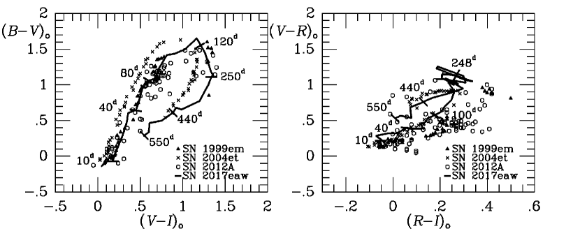
Figure 8: Comparison of the extinction-corrected colour-colour evolution of SN 2017eaw (dark solid curve) with the same evolutionary data for three other SN II-P. The tic marks indicate specific phases, which are labeled in days past the explosion date.

5 Bolometric Luminosity

5.1 Light Curve

The $BVRI$ light curves of SN 2017eaw can be used to estimate its bolometric luminosity as a function of time. This is useful for comparing the supernova’s evolution with available hydrodynamic models, to estimate the mass of ⁵⁶Ni synthesized in the explosion, and for singular comparisons with other supernovae where the individual light curves might be very different. Deriving a bolometric light curve for a supernova technically requires having light curves available not only in the optical realm, but also in the UV and IR realms. Since we only have four filters, the construction of a bolometric light curve for SN 2017eaw will depend on bolometric corrections deduced from observations and models of other well-observed supernovae.

Lusk and Baron (2017) describe several approaches to deriving a bolometric light curve for a supernova. We use three approaches here. In the first, we convert the extinction-corrected broadband magnitude at each epoch into a flux at the top of the atmosphere using the known flux zero points of the standard photometric systems. For $UBVRIJHKL$ (the Cousins-Glass-Johnson system), these zero points and their effective wavelengths are given in Table A2 of Bessell et al. (1998). Only the $R$-band in Table 4 has a measured magnitude at every epoch of our observations. For $B$, $V$, and $I$, linear interpolation was used to approximately fill in missing magnitudes. The integrated luminosity from $B$ ($\lambda_{eff}$ = 0.438 nm) to $I$ ($\lambda_{eff}$ = 0.798 nm) was derived at each epoch using the trapezoidal rule. This quasi-bolometric light curve is shown as the light solid curve in Figure 10.

The second approach we use is a colour-bolometric correction method. In this approach, well-observed supernovae are used to derive bolometric corrections to a specific filter light curve as a function of colour. These corrections are then fitted with a polynomial of relatively low order. Lyman et al. (2014) were able to derive a fairly well-defined parabolic relation between the $B$-band bolometric correction of Type II SNe and the extinction-corrected $(B-I)_{o}$ colour index,

$${\rm BC}_{B}=0.004-0.297(B-I)_{o}-0.149(B-I)_{o}^{2},$$

This is based on spectral energy distributions constructed from available light curves for 21 SNe, and which in general cover the period from early-on to the end of the plateau phase. The relation is limited in applicability to the colour range 0.0 $\leq$ $(B-I)_{o}$ $\leq$ 2.8, which is an issue for SN 2017eaw because of the strong colour evolution. Even with the high adopted reddening, a few of our epochs are close to or slightly exceed the upper limit of 2.8 (Figure 9). For the purpose of applying equation 4, the two parts of the $(B-I)_{o}$ evolution of SN 2017eaw were fitted with separate 6th or 7th order polynomials and joined at $(B-I)_{o}$ = 1.70 (solid curve in Figure 9), in order to give a smooth mapping of the evolution to 564 days.

The thick solid curve in Figure 10 is the bolometric light curve of SN 2017eaw based on equation 4 and Figure 9. The bolometric luminosity in ergs s^-1 is derived as

$$logL_{bol}=-0.4[B-A_{B}+{\rm BC}_{B}-5logD(cm)+8.74]$$

where $D$ is the distance in centimeters. The constant is based on an assumed absolute bolometric magnitude of the Sun of 4.74 (Bessell et al. 1998). Although equation 4 is technically valid only until the end of the plateau phase, Figure 10 shows how application of the BC_B polynomial to the full range of SN 2017eaw epochs (3 to 564 days) yields a bolometric light curve whose shape strongly resembles that of the quasi-bolometric light curve. As expected the colour-bolometric light curve is displaced towards higher values of $L_{bol}$ compared to the quasi-bolometric curve, since it accounts for missing flux in the UV and IR wavelength domains.

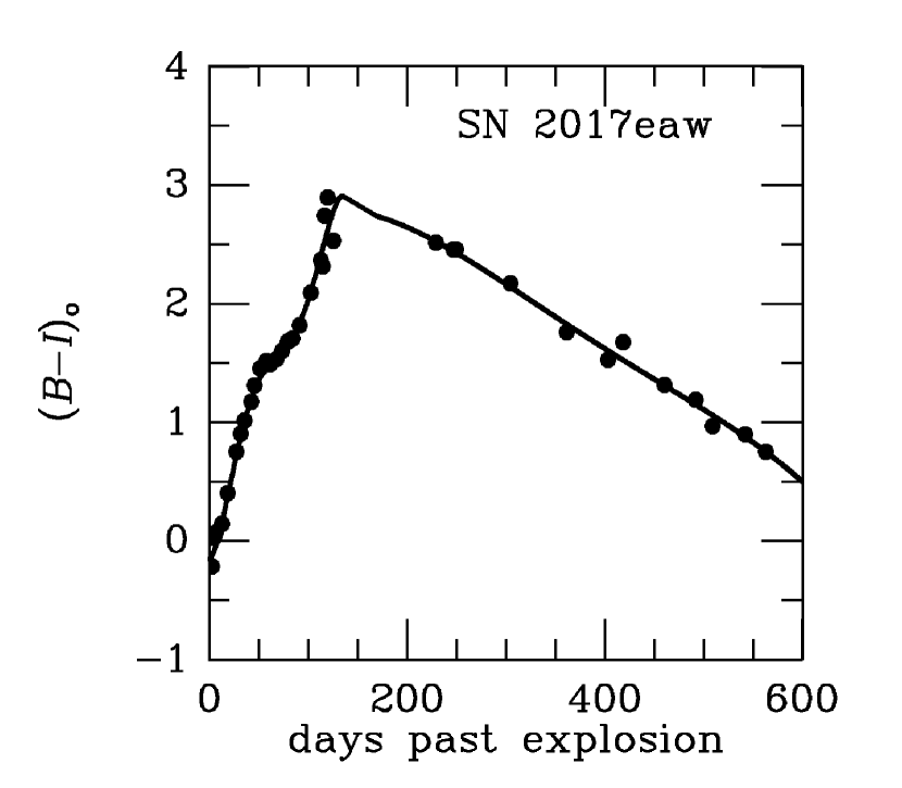
Figure 9: Polynomial representation of the $(B-I)_{o}$ evolution of SN 2017eaw. Two polynomials representing times before and after 170 days past the explosion date are combined and shown with the solid curve. Filled circles are from Table 4, corrected for an assumed total reddening of $E(B-V)$ = 0.41 mag.

The third approach uses bolometric corrections inferred from the well-observed supernova 2004et, which occurred in the same galaxy as SN 2017eaw and which we already have shown has $BVRI$ magnitude and colour evolutions very similar to SN 2017eaw. Maguire et al. (2010) presented extended observations of SN 2004et, and were able to derive bolometric corrections, BC($t$), relative to the $V$ and $R$ filters from $UBVRIJHKL$ observations taken $\approx$5 days to $\approx$120 days past the explosion. This covers only up to the end of the plateau phase. Maguire et al. (2010) cover the early tail to $\approx$190 days using observations of SN 1999em. We use the $R$-band calibration because it appears to be more homogeneous among different SNe compared to the $V$-band (Figures 8 and 9 of Maguire et al. 2010). The corrections were derived as

$$BC_{R}(t)=0.389+0.033t-4.27\times 10^{-4}t^{2}+1.80\times 10^{-6}t^{3}$$

and the resulting bolometric light curve was derived as

$$logL_{bol}=-0.4[R-A_{R}+{\rm BC}_{R}(t)-5logD(cm)+8.14]$$

This is shown as the short dotted curve in Figure 10. The constant 8.14 was used by Maguire et al. in the derivation of the bolometric corrections.

5.2 Mass of ⁵⁶Ni and other parameters

Having a bolometric light curve allows us to derive important physical parameters of SN 2017eaw. These can depend on choosing a particular time of reference, usually something connected with the end of the plateau phase or the beginning of the radioactive tail phase. These times are shown in Figure 11.

One set of parameters is described by Nakar et al. (2016); these include several useful quantities that are concerned with the relative importance of shock-deposited energy and the decay chain of ⁵⁶Ni on the appearance of the bolometric light curve. The period before the onset of the radioactive tail is believed to be dominated by photospheric emission. Nakar et al. note that ⁵⁶Ni emission could play a role on the appearance of the light curve during this phase, by either extending the plateau or flattening it. If the gamma rays produced by the ⁵⁶Ni decay chain are assumed to be fully confined and thermalized, then the mass of ⁵⁶Ni created in the explosion is directly proportional to the bolometric luminosity on the tail, which is assumed to be equal to the energy, $Q_{Ni}$, imparted to the ejected material by the steps in the ⁵⁶Ni decay chain. Nakar et al.’s equation 1 (see also Sutherland and Wheeler 1984) then gives the ⁵⁶Ni mass as:

$${{M(^{56}{\rm Ni})}\over M_{\odot}}={L_{bol}(t)\ \ \ {\rm[tail]}\over{6.45e^{-{t\over 8.8}}+1.45e^{-{t\over 111.3}}}}\times 10^{-43}$$

where $t$ is the time in days since the explosion. This can be applied at each epoch along the tail. The standard deviation of these points over a range of epochs measures how well the decay chain maps to the bolometric light curve.

Table 7 gives the ⁵⁶Ni mass implied by equation 8 for the three curves in Figure 10. The quasi-bolometric light curve gives an underestimate of 0.041$M_{\odot}$ for the ⁵⁶Ni mass. The bolometric curve based on equations 4 and 5 gives $M$(⁵⁶Ni)= 0.113_-0.017^+0.019$M_{\odot}$, while that based on equations 6 and 7 gives $M$(⁵⁶Ni)= 0.102_-0.019^+0.022$M_{\odot}$. With these estimates of the ⁵⁶Ni mass, we can derive other parameters discussed by Nakar et al. (2016) based on time-weighted averages from $t$ = 0 (explosion date) to $t$ = $t_{\rm Ni}$, the time of the beginning of the tail phase (Figure 11). These parameters are: $ET$, the time-averaged shock-deposited energy in units of 3$\times$10⁵⁵ erg s; $\eta_{Ni}$, the ratio of the time-weighted energy injected into the expanding gases due to the ⁵⁶Ni decay chain to $ET$; 2.5log$\Lambda_{e}$, a parameter telling how fast the decline and duration of the bolometric light curve would be in the absence of any ⁵⁶Ni emission; and $\Delta M_{25-75}$, a measure of the decline rate in magnitudes of the bolometric luminosity from day 25 to day 75. $ET$ is an important parameter that is discussed in more detail by Shussman et al. (2016), who show that ET $\propto$ $E_{exp}$${}^{1\over 2}$ $R_{*}$ $M_{ej}$${}^{1\over 2}$, where $E_{exp}$ is the explosion energy, $R_{*}$ is the pre-explosion progenitor radius, and $M_{ej}$ is the mass of the ejecta.

Table 7: Nakar et al. (2016) parameters. Col. 1: parameter from Nakar et al. (2016); cols. 2-4: values of parameters for the curves in Figure 10; col. 5: mean and standard deviation of the same parameters for 13 SNe listed in Table 1 of Nakar et al.

Parameter	Value	Value	Value	mean Nakar
bolometric type	$BVRI$	BCB	BCR	bolometric
1	2	3	4	5
Mass Ni56/$M_{\odot}$	0.041	0.113-0.017+0.019	0.102-0.019+0.022	0.031$\pm$0.018
$ET$	1.25	2.27	2.43	1.03$\pm$0.67
$\eta_{Ni}$	0.50	0.76	0.64	0.56$\pm$0.63
2.5log$\Lambda_{e}$	0.73	0.91	0.87	0.79$\pm$0.33
$\Delta M_{25-75}$	0.29	0.34	0.37	0.40$\pm$0.38

Table 8: Litvinova and Nadyozhin (1985) parameters

Parameter	Value
1	2
Explosion energy	15.9-1.1+1.3$\times$1050 ergs
Mass of ejected envelope	20-3+2$M_{\odot}$
Pre-supernova radius	536-150+200$R_{\odot}$

The values of these parameters derived for SN 2017eaw are listed in Table 7 and, at least for $\eta_{Ni}$, 2.5log$\Lambda_{e}$, and $\Delta M_{25-75}$, are within the ranges found for 13 other SNe by Nakar et al. (2016, their Table 1), with $ET$ and $\eta_{\rm Ni}$ being near the higher ends of their ranges. The last column of Table  7 lists the mean and standard deviation of the Nakar et al. Table 1 values for comparison. As noted by Nakar et al., these parameters are less sensitive to the difference between a bolometric and quasi-bolometric light curve than is the ⁵⁶Ni mass. The high value, $\eta_{\rm Ni}$ = 0.76, obtained for the BC${}_{B}(B-I)$ bolometric light curve implies that ⁵⁶Ni contributed 43% of the time-weighted integrated luminosity of SN 2017eaw during its plateau/photospheric emission phase. For the $BC_{R}(t)$ curve, the contribution is 39%. These should be compared with the typical value of $\approx$30% for bolometric curves derived by Nakar et al. (2016). Nakar et al. (2016) also derive these parameters for the quasi-bolometric light curves of several SNe. For SN 2017eaw we find $\eta_{\rm Ni}$ = 0.50, which compares very well with the average value, 0.49, for 5 other supernovae with only $BVRI$ photometry (Nakar et al., their Table 2).

The main difference with the Nakar et al. sample is the estimated mass of ⁵⁶Ni. The bolometric curve values in Table 7 are $\approx$3.5 times higher than the average of the Nakar et al. sample, and nearly twice the hightest value listed in their Table 1.

Another estimate of the ⁵⁶Ni mass for SN 2017eaw can be made based on the correlation between the absolute $V$-band magnitude on the plateau and the ⁵⁶Ni mass (Hamuy 2003). Elmhamdi et al. (2003) discuss the correlation and use 8 SNe to derive

$$log{M(^{56}Ni)\over M_{\odot}}=-0.438M_{V}^{o}(t_{i}-35)-8.46$$

where $t_{i}$ is the time when the dropoff rate at the end of the plateau phase in the $V$-band is maximal (see Figure 11), and $M_{V}^{o}(t_{i}-35)$ is the corrected absolute magnitude 35 days before that point in time. From our $V$-band light curve directly, we derive $t_{i}$ = 117$\pm$3 days and $M_{V}^{o}$ = $-$17.36$\pm$0.04, for which the above equation gives $M$(⁵⁶Ni) = 0.139_-0.031^+0.039$M_{\odot}$, accounting also for the uncertainty in extinction and distance. This is about 25% larger than the ⁵⁶Ni mass derived from the bolometric light curves in Figure 10. Note that Elmhamdi et al. (2003) also show that the slope, $S$, at $t_{i}$ also correlates with $logM(^{56}Ni)$: the larger the value of $S$, the lower the ⁵⁶Ni mass. Directly from our $V$-band light curve, we get $S$ $\approx$0.14 mag day^-1, which by equation 2 of Elmhamdi et al. (2003) yields $M$(⁵⁶Ni) = 0.021$M_{\odot}$, considerably less than the value implied by the $V$-band magnitude on the plateau. Our $V$-band light curve may not be well-sampled enough to obtain a reliable value of $S$.

Hamuy (2003) uses the $V$-band luminosity on the tail and a fixed bolometric correction of 0.26$\pm$0.06 mag to estimate the ⁵⁶Ni mass. Hamuy’s equations 1 and 2 applied to our $V$-band light curve from 126 to 290 days gives $M$(⁵⁶Ni) = 0.106_-0.022^+0.027$M_{\odot}$.

Thus, for the distance and reddening we have adopted, and their uncertainties, the implied ⁵⁶Ni mass for SN 2017eaw is 0.115_-0.022^+0.027$M_{\odot}$. This is $\approx$30% larger than the amount inferred to have been created in the SN 1987A explosion (Arnett 1996) but is within the ranges found by Hamuy (2003) and Elmhamdi et al. (2003). This value is also in good agreement with Sahu et al.’s (2006) estimate of 0.06$\pm$0.02 $M_{\odot}$ for SN2004et, which, when scaled to our adopted distance, becomes 0.11$\pm$0.03$M_{\odot}$.

Litvinova and Nadyozhin (1985; see also Nadyozhin 2003) used models of Type II-P SNe to derive relations connecting the energy of the explosion, the amount of mass ejected, and the pre-explosion radius of the star to observable parameters, including the absolute magnitude $M_{V_{p}}^{o}$ in the middle of the plateau, the expansion velocity at this time, and the time, $\Delta t$, during which the SN was within $\pm$1.0 mag of $V_{p}$. The latter parameter is schematically shown in Figure 11. Using Figure 9 of Szalai et al. (2019), we estimate the expansion velocity for SN 2017eaw to have been 4200 km s^-1 at $\approx$60 days past explosion, based on the Fe II 5169 line. The results are summarized in Table 8. The explosion energy and pre-supernova radius are found to be 15.9_-1.1^+1.3$\times$10⁵⁰ ergs and 536_-150⁺²⁰⁰$R_{\odot}$, respectively. However, the ejected mass, 20_-3⁺² $M_{\odot}$, greatly exceeds recent estimates of the total mass of the progenitor of SN 2017eaw (section 6). Hamuy (2003) discusses the limitations of the Litvinova and Nadyozhin (1985) formulae, which include assuming no contribution to the plateau luminosity by ⁵⁶Co decay, difficulties in estimating the photospheric velocity on the plateau, and the assumption that Type II-P supernovae have blackbody spectra.

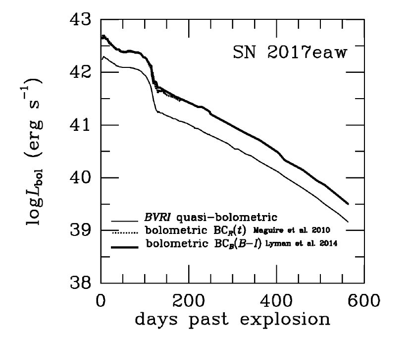
Figure 10: The thin solid curve is based on trapezoidal integration of the interpolated $BVRI$ light curves. The thick solid curve shows the bolometric light curve based on the absolute $B$-band light curve and a quadratic representation (Lyman et al. 2014) of the bolometric correction using the corrected colour index, $(B-I)_{o}$, the mapping of which is shown in Figure 9. The dotted curve is the bolometric light curve based on the absolute $R$-band magnitude and a time-dependent bolometric correction (Maguire et al. 2010).

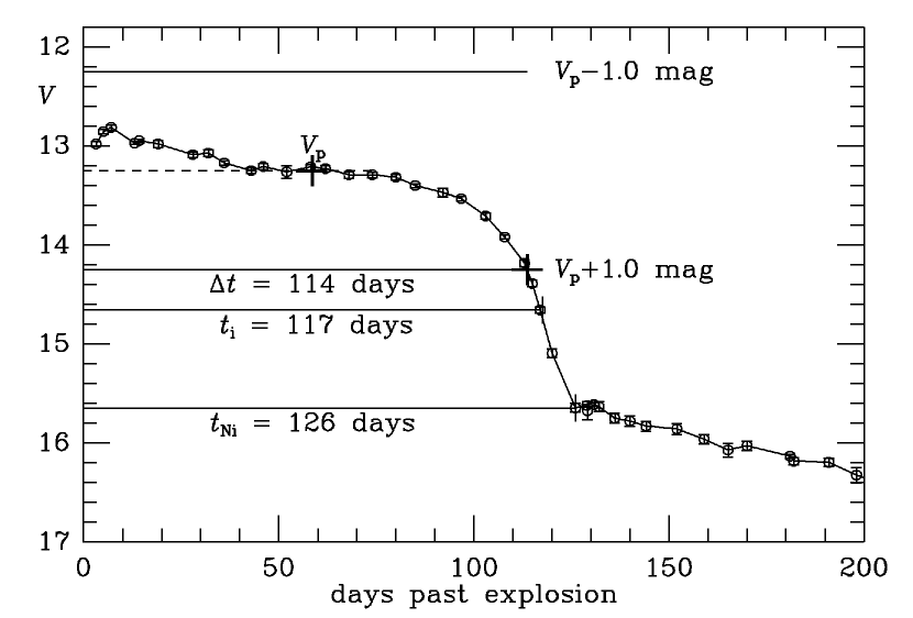
Figure 11: Schematic of aspects of the early light curve of a typical Type II-P SN, showing how certain times are defined (see text).

6 The Supernova Progenitor

SN 2017eaw is one of only a few SNe for which the progenitor has been identified. Kilpatrick and Foley (2018) describe the detection of the likely progenitor in Hubble Space Telescope and Spitzer Space Telescope data up to 13 years before the explosion. These authors estimate that the progenitor was a red supergiant having an initial (zero age main sequence) mass of 13_-2⁺⁴ $M_{\odot}$. This is based on an assumed distance of 6.72 Mpc, and would correspond to 14_-3.5⁺³ $M_{\odot}$ for the distance, 7.72 Mpc, that we have adopted (Eldridge and Xiao 2019).

Rui et al. (2019) used nine archival HST images of the site of SN 2017eaw to measure the photometric properties of the progenitor. These images were obtained at epochs in 2004, 2016, and 2017, with the majority in 2016. Photometry in different filters was used to determine the progenitor to be an M4 supergiant with a surface temperature of 3550$\pm$100K and radius of 575$\pm$120$R_{\odot}$. With this and an estimate of the bolometric luminosity, Rui et al. used an H-R diagram to obtain a progenitor ZAMS mass of 10-14$M_{\odot}$. This value assumes a distance of 5.5 Mpc and an extinction $A_{V}$ = 1.83$\pm$0.59 mag, compared to our adopted values of 7.72 Mpc and 1.27 mag, respectively. The increase in distance modulus by 0.77 mag is only partly compensated by the reduction in $A_{V}$ of 0.56 mag. If these latter values were used, the estimated progenitor mass would increase somewhat. Using pre-explosion HST and Spitzer data and a distance of 7.73 Mpc, Van Dyk et al. (2019) estimated a progenitor mass of 15$M_{\odot}$.

Kilpatrick and Foley (2018) also found evidence for a pre-explosion circumstellar dust shell about 4000$R_{\odot}$ in radius. Rui et al. (2019) concluded that the formation of such a shell by mass loss a few years prior to explosion could have caused an observed reduction in brightness in 2016. However, Johnson et al. (2018) also examined HST images of the progenitor and found little or no evidence for significant variability within 9 years before the explosion. These authors also show that the progenitors for three other Type II SNe similarly show no evidence for significant pre-explosion variability.

7 Summary

We have presented $BVRI$ light curves of the classic Type II-P supernova 2017eaw, the tenth supernova discovered in NGC 6946 in 100 years. Our main findings are:

1. The $BVRI$ light and colour curves of SN 2017eaw show all the classic features of a typical Type II-P supernova.

2. These curves strongly resemble those of SN 2004et, another Type II-P SN that appeared in the same galaxy.

3. SN 2017eaw reached an absolute $V$-band magnitude of $-$17.9, based on an assumed distance of 7.72 Mpc and a reddening of $E(B-V)$ = 0.41$\pm$0.05, and was slightly less luminous than SN 2004et on the plateau in all four filters.

4. The decline in brightness on the early part of the “tail" is consistent with ithe luminosity being powered by radioactive decay of ⁵⁶Co into ⁵⁶Fe. This is true mainly for the $VRI$ filters, and less so for the $B$-band.

5. The slope of the tail increases past 290 days, possibly indicating the gradual breakdown of the confinement and thermalization assumption of the gamma rays released by the radioactivity (Arnett 1996).

6. Using several approaches, we have estimated that 0.115_-0.022^+0.027$M_{\odot}$ of ⁵⁶Ni was produced in the explosion of SN 2017eaw, a higher than average but not extreme value.

7. The ⁵⁶Ni decay chain contributed 43% of the time-averaged bolometric luminosity over the period from 0 to 117 days past the explosion date (estimated to have occurred on JD 2457886.5). The remaining 57% is due to the shock-deposited energy from the explosion itself that dominates the plateau phase.

8. The star that exploded was a red supergiant having an estimated pre-explosion radius of 536_-150⁺²⁰⁰$R_{\odot}$. The explosion energy was about 1.6$\times$10⁵¹ ergs. The actual progenitor has been identified in pre-explosion images.

We thank the referee for helpful comments that improved this paper. This research has made use of the NASA/IPAC Extragalactic Database (NED) which is operated by the Jet Propulsion Laboratory, California Institute of Technology, under contract with the National Aeronautics and Space Administration.

8 Appendix

Because NGC 6946 is such a prolific producer of SNe, several published sources having photometry of local field stars are available for comparison with our Table 2 system. One source, Buta (1982), has only $UBV$ photometry, but Table 1 of that paper includes 10 stars in common with Table 3. Botticella et al. (2009) present $UBVRI$ photometry of 26 numbered stars they used for photometry of SN 2008S, of which 5 are included in Table 3. These authors observed the same local standards as did Pozzo et al. (2006), but added $U$ and $B$. Sahu et al. (2006) based their photometry of SN 2004et on 8 local standards, only 1 of which overlaps Table 3. In order to include the Sahu et al. photometry in our comparison, Table 9 lists the magnitudes and colours of the eight Sahu et al. local standards using the same images and the same transformation and extinction coefficients as were used for the stars in Table 3. All are faint standards and Sahu stars 6-8 have an especially low signal-to-noise compared to most of the stars in Table 3. Our comparison is based on Sahu et al. stars 1-5.

The results are summarized in Table 10. In general, we find that the mean differences between the other sources and the photometric system represented by Table 3 are generally less than $\pm$0.04 mag. Because NGC 6946 is likely to host many more SNe, we anticipate improving the Table 3 photometric system in future studies.

Table 9: Photometry of local standards used by Sahu et al. (2006)

Sahu et al.	$V$	$B-V$	$V-R$	$R-I$
No.	m.e.	m.e.	m.e.	m.e.
1	2	3	4	5
1	15.185	0.731	0.501	0.433
	0.044	0.108	0.061	0.028
2	13.772	0.660	0.430	0.411
	0.015	0.040	0.014	0.012
3	14.262	1.367	0.716	0.665
	0.020	0.109	0.028	0.013
4	14.740	0.728	0.500	0.479
	0.017	0.053	0.012	0.020
5	14.833	0.793	0.483	0.492
	0.028	0.051	0.028	0.021
6	16.118	0.978	0.708	0.563
	0.156	0.289	0.131	0.037
7	16.401	0.604	0.537	0.513
	0.067	0.101	0.082	0.025
8	16.400	0.468	0.549	0.391
	0.074	0.246	0.100	0.040

Table 10: Comparisons of Table 3 system magnitudes with published local photometry from Buta (1982), Sahu et al. 2006, and Botticella et al. (2009). The sense is $\Delta$ = (published values) $-$ (Table 3 system values).

Filter/colour	$<\Delta>$	$<\Delta>$	$<\Delta>$
	Buta 1982	Sahu et al.	Botticella et al.
1	2	3	4
$B$	0.018$\pm$0.009	$-$0.036$\pm$0.032	$-$0.037$\pm$0.041
$V$	$-$0.002$\pm$0.005	$-$0.021$\pm$0.011	$-$0.019$\pm$0.019
$R$	………………	0.004$\pm$0.007	0.020$\pm$0.006
$I$	………………	0.006$\pm$0.012	0.037$\pm$0.008
$B-V$	0.020$\pm$0.007	$-$0.016$\pm$0.032	$-$0.019$\pm$0.031
$V-R$	………………	$-$0.025$\pm$0.005	$-$0.039$\pm$0.021
$R-I$	………………	$-$0.002$\pm$0.008	$-$0.017$\pm$0.011
$n$	10	5	5

References

- (1) Anand G. S., Rizzi L., Tully R. B., 2018, AJ, 156, 105
- (2) Arnett D., 1996, Supernovae and Nucleosynthesis: An Investigation of the History of Matter from the Big Bang to the Present, Princeton, Princeton University Press
- (3) Bessell M. S., Castelli F., Plez B., 1998, A & A, 333, 231
- (4) Botticella M. T., et al., 2009, MNRAS, 398, 1041
- (5) Branch D., Wheeler J. C., 2017, Supernova Explosions, Berlin, Springer
- (6) Buta R., 1982, PASP, 94, 578
- (7) Buta R., Corwin H., Odewahn S., 2007, The de Vaucouleurs Atlas of Galaxies, Cambridge, Canbridge University Press (deVA)
- (8) Cardelli J. A., Clayton G. C., Mathis J. C., 1989, ApJ, 345, 245
- (9) de Vaucouleurs G., de Vaucouleurs A., Corwin H. G., Buta R. J., Paturel G., Fouque P., 1991, Third Reference Catalogue of Bright Galaxies, New York: Springer (RC3)
- (10) Dong S., Stanek K. Z., 2017, The Astronomer’s Telegram, 10372
- (11) Eldridge J., Xiao L., 2019, MNRAS, 485, L58
- (12) Elmhamdi A., Chugai N. N., Danziger I., 2003, A&A, 404, 1077
- (13) Hamuy M., 2003, ApJ, 582, 905
- (14) Jerkstrand A., 2011, PhD Thesis, University of Stockholm
- (15) Johnson S. A., Kochanek C. S., Adams S. M., 2018, MNRAS, 480, 1696
- (16) Keel W. C., Oswalt T., Mack P., et al., 2017, PASP, 129, 015002
- (17) Kilpatrick C. D., Foley R. J., 2018, MNRAS, 481, 2536
- (18) Landolt A., 1992, AJ, 104, 340
- (19) Litvinova I. Y., Nadyozhin D. K., 1985, Sov. Astron. Lett., 11, 145
- (20) Leonard D. C., et al., 2002, PASP, 114, 35
- (21) Li W., et al. 2011, MNRAS, 412, 1441
- (22) Lusk J. A., Baron E., 2017, PASP, 129, 044202
- (23) Lyman J. D., Bersier D., James P. A., 2014, MNRAS, 437, 3848
- (24) Macguire K., et al., 2010, MNRAS, 404, 981
- (25) Munari U., Zwitter T., 1997, A&A, 318, 269
- (26) Nakar E., Poznanski D., Katz B., 2016, ApJ, 823, 127
- (27) Nadyozhin D. K., 1994, ApJS, 92, 527
- (28) Otsuka M., et al., 2012, ApJ, 744, 26
- (29) Pozzo M., et al., 2006, MNRAS, 369, 1169
- (30) Rui L., et al. , 2019, MNRAS, 485, 1990
- (31) Sahu D. K., Anupama G. C., Srividya S, Muneer S., 2006, MNRAS, 372, 1315
- (32) Schlafly E. F., Finkbeiner D. P., 2011, ApJ, 737, 103
- (33) Shussman T., Nakar E., Waldman R., Katz B., 2016, arXiv 1602.02774
- (34) Silverman J. M., et al., 2017, MNRAS, 467, 369
- (35) Smartt S. J., 2009, ARAA, 47, 63
- (36) Smartt S. J., Eldridge J. J., Crockett R. M., Maund J. R., 2009, MNRAS, 395, 1409
- (37) Stritzinger, M., et al. 2002, AJ, 124, 2100
- (38) Suntzeff N. B., et al., 1988, AJ, 96,1864
- (39) Sutherland P. G., Wheeler J. C., 1984, ApJ, 280, 282
- (40) Szalai T., et al., 2019, arXiv 1903.09048
- (41) Tomasella L., et al., 2013, MNRAS, 434, 1636
- (42) Tomasella L., et al., 2017, The Astronomer’s Telegram, 10377
- (43) Tsvetkov D. Yu. et al., 2018, AstL, 44,315
- (44) Van Dyk S. D., et al., 2019, arXiv 1903.03872
- (45) Wiggins P. 2017, CBET, 4391, 2
- (46) Woosley S. F., Hartmann D., Pinto P. A., 1989, ApJ, 346, 395
- (47) Zwitter T., Munari U. Moretti S., 2004, IAU Circular 8413, 1