Molecules with dipoles in periodic boundary conditions in a tetragonal cell

Abstract

When a system which contains a dipole, and whose dimensionality is less than three, is studied in a code which imposes periodic boundary conditions in all three dimensions, an artificial electric field arises which keeps the potential periodic. This has an impact on the total energy of the system, and on any other attribute which would respond to an electric field. Simple corrections are known for 0D systems embedded in a cubic geometry, and 2D slab systems. This paper shows how the 0D result can be extended to tetragonal geometries, and that for a particular $c/a$ ratio the correction is zero. It also considers an exponential error term absent from the usual consideration of 2D slab geometries, and discusses an empirical form for this.

1 Introduction

Plane-wave electronic structure codes enforce periodicity in all three dimensions. Whilst this is ideal for studying bulk crystals, it can cause complications when the system of interest has lower dimensionality, such as a surface (2D), a nanowire (1D), or an isolated molecule (0D). In order to study these systems in such codes, a region of vacuum is used to separate the system from its fictitious periodic images. As the extent of the vacuum is increased, properties converge to the values that they would have in the absence of the imposed periodicity.

Large amounts of vacuum significantly increase the memory and time costs of calculations, so it is useful to be able to apply corrections which accelerate the convergence with vacuum size. This paper considers the interactions arising from dipole–dipole interactions in charge-neutral systems. In such systems, this interaction decays the most slowly with system size.

For the 2D geometry of a slab of material, commonly used to study surfaces, a dipole moment perpendicular to the slab results in a compensating electric field in order to keep the potential periodic[1]. A 2D slab with a perpendicular dipole moment is effectively a charged parallel plate capacitor, and one would expect the potential on each side to differ, and the field outside the plates to be zero. This is not consistent with the potential being zero at infinity, so a compensating field arises automatically.

A simple, effective, but computationally-expensive, solution to this problem is to use a simulation cell consisting of two slabs in opposite orientations so that the total dipole moment is zero.

A self-consistent correction adds an equal and opposite field within the simulation. This can be done by placing the required discontinuity in the potential in the vacuum region[1, 2]. Many DFT codes include this approach[3, 4, 5].

A post hoc correction simply involves adding a term to the final energy. This make no improvement to the convergence of other properties of the system, such as dipole moments or bond lengths, but does significantly improve the energy. The energy correction is

$$\Delta E_{\textrm{slab}}=\frac{p^{2}}{2\epsilon_{0}V}$$ (1)

where $p$ is the dipole moment, which must be perpendicular to the slab, and $V$ the unit cell volume[2]. The electric field arising is simply $\mathbf{p}/\epsilon_{0}V$. These corrections decay as the reciprocal of the slab separation. These three schemes are discussed in more detail in reference [6].

Similar expressions arise for the 0D geometry of a molecule in a cubic box[7, 8], save that they have an extra prefactor of a third,

$$\Delta E_{\textrm{cube}}=\frac{p^{2}}{6\epsilon_{0}V}$$ (2)

and a field correction of $\mathbf{p}/(3\epsilon_{0}V)$. These corrections for the cubic geometry are referred to later as the Makov-Payne correction[8].

More general geometries have been considered[7, 8, 9], and extended to systems embedded in anisotropic dielectrics[10], but these tend to result in a requirement to perform a infinite lattice sum, rather than a simple rational prefactor.

Other methods have been considered to correct for unwanted dipole-dipole interactions. These include the truncation of the Coulomb potential in real space[11], which was proven to be equivalent to the above self-consistent slab correction[12]. However, Coulomb truncation methods require the extent of the vacuum region to be greater than the extent of the non-vacuum region[13]. Sharp cut-offs, and ‘minimum image’ modifications, to the Coulomb potential are compared in detail in Ref [14].

For the slab geometry a different approach is to use a 2D version of the Ewald sum[15]. This has also shown to be equivalent to the 3D Ewald sum with the above slab correction[16].

This paper considers a limited generalisation of the cube result of Makov and Payne, a generalisation which avoids the need for summations, and it considers a particular geometry for which no correction is needed. It also finds a further correction term for the 2D slab geometry.

2 Tetragonal Cells

The corrections described above relate calculation cells to an ideal cell in which one, or more, of the repeat distances has been extended to infinity. The geometry for which further results can be readily obtained is the 0D system of a molecule in a tetragonal cell with the molecule’s dipole moment parallel to the $\mathbf{c}$ axis, the cell volume being $V=a^{2}c$.

Equation 1 allows one to calculate the energy change arising from the dipole interaction between the periodic images of the simulation cell if $c$ were increased to infinity. It also allows one to calculate what the energy would be in another simulation cell with a different value of $c$, by first increasing to infinity, and then reducing to the new value. So one can consider what the dipole-dipole interaction energy would have been had the calculation been performed in a cubic cell, one with $c=a$, albeit ignoring the warning given by Yeh and Berkowitz[17] that the slab correction loses accuracy unless the vacuum gap size exceeds $a$. The correction would be:

$$\Delta E=\frac{p^{2}}{2\epsilon_{0}a^{2}c}-\frac{p^{2}}{2\epsilon_{0}a^{3}}$$ (3)

Now that the cell is cubic, one can apply equation 2 to expand $a$ to infinity in a cubic geometry, giving

$$\Delta E=\frac{p^{2}}{2\epsilon_{0}a^{2}c}-\frac{p^{2}}{2\epsilon_{0}a^{3}}+\frac{p^{2}}{6\epsilon_{0}a^{3}}$$ (4)

which simplifies to

$$\Delta E_{\textrm{tetragonal}}=\frac{p^{2}}{\epsilon_{0}a^{2}}\left(\frac{1}{2c}-\frac{1}{3a}\right)$$ (5)

This is thus the energy correction arising from dipole-dipole interactions required to expand a charge-neutral, finite, tetragonal cell with the dipole moment wholly along the $\mathbf{c}$ axis to infinite size. It is zero if $c=1.5a$.

That the energy correction is zero implies that the correcting field that should be added in a self-consistent calculation will also be zero, and repeating the above calculations for the field rather than the energy confirms this.

So by careful choice of the 3D simulation cell geometry one can cause the dipole-dipole interaction for a 0D system to cancel, even in a code with no built-in correction.

3 Calculations

In order to demonstrate the above theory, some calculations were performed on a KCl molecule using Castep[3], and the dipole moments and post hoc corrections calculated with c2x[18]. As only the convergence of properties with cell size was of interest, little thought was given to the choice of exchange-correlation functional or pseudopotential, save that a single-electron pseudopotential was used for K for its speed benefits. The bond length was fixed at 2.7Å.

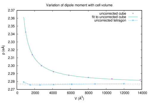
Figure 1: Variation of dipole moment of KCl molecule in a cubic box, and a tetragonal box with $c=1.5a$. For the cubic box, the crosses represent calculations, and the line is a best-fit of constant plus a decay inversely proportional to volume. The horizontal dotted line is the asymptote of this fit.

First the dipole moment of the KCl molecule was considered. In a cubic cell the effect of the periodic images will be to produce a field which enhances the dipole moment through polarisation, and this field should decay as the reciprocal of the cell volume. In a tetragonal cell with $c=1.5a$, this field is expected to be zero, and therefore the convergence with cell size is expected to be much faster.

The results from uncorrected cubic cells are shown in figure 1, together with a fitted line of the form $\alpha+\beta/V$ where $V$ is the cell volume. The value of $\alpha$ is 2.27688eÅ. The same calculation was performed in tetragonal boxes with $c=1.5a$ and $c$ being 15, 18, 24 and 30Å. The results from the tetragonal cell show very little variation with cell volume, and lie close to the value obtained by extrapolating the curve fitted to the cubic data to infinite volume. A 10Åx10Åx15Å tetragonal box gives about one fifth of the error of the cube of side 24Å, in a cell of little more than one tenth of the volume.

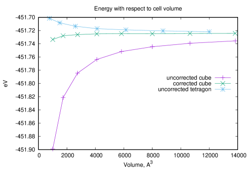
Figure 2: Variation of the energy of a KCl molecule in cubic and tetragonal (c=1.5a) boxes of various volumes.

The energy convergence is also improved by the use of a tetragonal cell, but is found to be less good than a cubic cell with the correction of equation 2. This is shown in figure 2, where the x-axis is now volume to give a fairer comparison between cubic and tetragonal cells. Whilst the use of a tetragonal cell is a significant improvement over an uncorrected cubic cell, attempts to fit equations to the remaining error show that a small term inversely proportional to the volume remains.

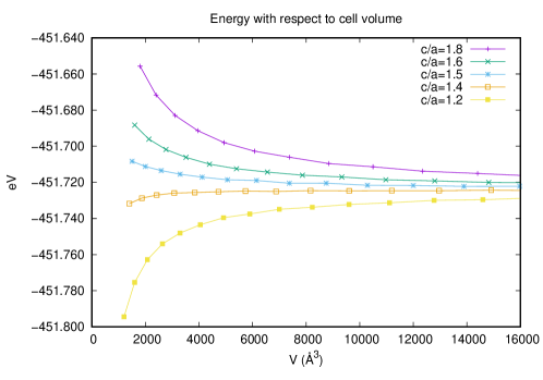
Figure 3: Variation of the energy of a KCl molecule in tetragonal boxes of various $c/a$ ratios and different volumes.

If the variation of energy at different $c/a$ ratios is considered, as presented in figure 3, then the movement from the dominant term being a lowering of energy from the attractive interactions in the $c$ direction at low values of $c/a$ to the rise in energy as the repulsive interactions perpendicular to $c$ at higher values of $c/a$ is clear. However, cancellation of these effects appears to occur at a value of $c/a$ only very slightly greater than 1.4, and not at 1.5 as this section would suggest. The following section explores the reason for this.

4 The Slab Correction Revisited

The theory of the slab correction is usually expressed in terms of parallel plate capacitors. In the periodic system, the planes half-way between the slabs have constant potential. If a thin conducting sheet were placed in one such plane, then the two halves of the system would no longer be influenced by each other, but each would see in the sheet a set of mirror charges which would be identical to the now-shielded half of the system. Hence such conducting sheets may be introduced without changing the system.

A capacitor of plate separation $d$ and surface charge density $\sigma$ has a dipole moment per unit area of $\sigma d$, a field between the plates of $\sigma/\epsilon_{0}$, and a potential difference of $\sigma d/\epsilon_{0}$. So it is argued that in the simulation cell a potential difference of $p/\epsilon_{0}A$ would be expected, where $p$ is the dipole moment perpendicular to the slab, and $A$ the cell’s area in the plane of the slab. That periodic boundary conditions apply to the potential forces the removal of this potential difference by the imposition of an artificial field of magnitude $p/\epsilon_{0}V$. The corrections of equation 1 and the corresponding field correction account for this unwanted electric field.

This leaves many terms unaccounted for: dipole moments parallel to the slab, quadrapole and higher moments, polarisation effects, and effects from the finite extent of dipoles as the theory applies to point dipoles. However, there are also terms arising purely from the static dipole which are not properly addressed.

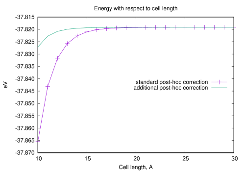
Figure 4: Variation of the post-hoc corrected Ewald slab energy with varying slab separation for a system of two point charges separated by 1.5Å in the centre of a teragonal cell with a=10Å and c varying. The line with points shows calculated values, and the bare line shows the result of adding the second correction proposed in equation 6.

It is instructive to consider a simpler system than the KCl molecule of the previous system, that of the Ewald energy of two equal and opposite point charges in a cell. The Ewald routine from the python package pymatgen[19] was used for this. The system was two charges of $+2e$ and $-2e$ separated by 1.5Å in a tetragonal box with $a=$10Å and $c$ varying from 5Å to 50Å. The energy of this system for part of this range, corrected by equation 1, is shown in figure 4. Also shown in the figure is the result of adding a second empirical correction term of

$$\delta E=\frac{4\pi p^{2}}{\epsilon_{0}a^{3}}\exp(-2\pi c/a)$$ (6)

This correction was found to fit data well for various configurations of the test system, with the fit improving as the separation of the charges was reduced. Whilst the author is unable to offer analytic proof of the above form, the following observations can be made.

The electrostatic potential in a plane above and parallel to an isolated square array of dipoles is not a constant. Close to the slab it will vary as one moves from being close to a dipole in the slab to being between dipoles. The arguments based on capacitors assume that the potential is constant, as it would be if the dipole moment were uniformly distributed across the area of the slab, and also as it is far from the slab. Any variation in the potential $\phi$ in the vacuum region must obey Laplace’s equation of $\nabla^{2}\phi=0$. The variation parallel to the slab will have an oscillatory form with the longest wavelength component being $\exp(2\pi ix/a)$, leading to a decay away from the slab of the form $\exp(-2\pi z/a)$. This is the justification offered for the $\exp(-2\pi c/a)$ term in equation 6.

Dimensionality suggests the factor of $p^{2}/\epsilon_{0}$ and also the reciprocal of a volume. That the volume appears as $1/a^{3}$ not $1/a^{2}c$ is merely because that fitted the data very much better. The final factor of $4\pi$ arises simply from coercing a fitted constant to the nearest likely number.

Other exponentially decaying terms are to be expected, corresponding to shorter-wavelength components of the variation of the potential parallel to the plane, but the term quoted above will be the most slowly decaying. If the dipole were smeared out in the plane of the slab, and thus had the geometry of a parallel plate capacitor, then this correction term would not apply.

The same Ewald calculations with pymatgen can be performed in cubic cells. In this case the residual error after applying the traditional Makov-Payne correction was well fitted by a function decaying as $1/a^{5}$ as expected.

4.1 Returning to the Tetragonal Cell

When the slab geometry is considered, the additional correction proposed in equation 6 decays exponentially with cell length. In the case of a tetragonal cell in which $c/a$ is fixed as the cell size is varied, it merely decays as $1/V$. For the two shapes of tetragonal cell considered in this paper, that of $c=a$ (a cube), and $c=1.5a$, it takes the approximate values

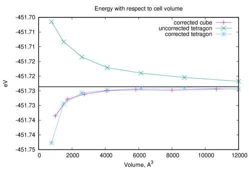
Figure 5: Variation of the energy of a KCl molecule in tetragonal (c=1.5a) boxes of various volumes, with and without the correction term proposed in this paper. The horizontal line is a guide to an extrapolation of the two datasets. The corrected cubic result from figure 2 is given for comparison, and lies above the corrected tetragonal result at 1000ų

$$\delta E_{\textrm{cube}}=0.0235\frac{p^{2}}{\epsilon_{0}V}$$ (7)

and

$$\delta E_{\textrm{tetragonal}}=0.0015\frac{p^{2}}{\epsilon_{0}V}$$ (8)

The arguments from equation 5 which stated that there was no energy correction term for $c/a=1.5$ neglected this correction, and so there does remain a correction of

$$\delta E=\frac{4\pi p^{2}}{\epsilon_{0}a^{3}}\left(\exp(-2\pi)-\exp(-3\pi)\right)$$ (9)

This can now be applied to figure 2 to produce figure 5. This shows that such a term improves convergence, and gives very similar results to those obtained from a cubic cell with its post hoc correction. Given that equation 5 relies on equation 2 for the post hoc correction of a cubic cell, it would not be expected to perform better than this.

The leading term in the error in equation 2 arises from the non-zero length of the dipole which produces a term which decays as $1/a^{5}$. The energy of an isolated dipole of two charges $\pm q$ separated by $r$ is $-q^{2}/(4\pi\epsilon_{0}r)$, or $-p^{2}/(4\pi\epsilon_{0}r^{3})$. This term becomes large as the separation is reduced at constant dipole magnitude and dominates the Ewald sum. The finite precision of double precision arithmetic then prevents precise calculation of the interaction energies between adjacent dipoles by considering the differences in the Ewald energies of the systems.

Figure 3 showed that the best convergence of energy with respect to $c/a$ ratio was found at $c/a$ just over 1.4, and not at exactly 1.5. However, the best $c/a$ ratio for converging the energy is not expected to be found by setting equation 5 to zero and solving

$$\frac{p^{2}}{\epsilon_{0}a^{3}}\left(\frac{a}{2c}-\frac{1}{3}\right)=0$$ (10)

but rather by considering also the correction of equation 6 and solving

$$\frac{p^{2}}{\epsilon_{0}a^{3}}\left(\frac{a}{2c}-\frac{1}{3}\right)-\frac{4\pi p^{2}}{\epsilon_{0}a^{3}}\left(\exp(-2\pi)-\exp(-2\pi c/a)\right)=0$$ (11)

This has a numerical solution of $c/a\approx 1.4085$, which is consistent with figure 3. However, this $c/a$ ratio will not result in no correcting electric field, and thus will not produce the best results for the dipole moment, nor for other properties which will be influenced by such a field.

5 Conclusions

The well-known analytic corrections for dipole-dipole interactions for a molecule in a cubic box with periodic boundary conditions have been generalised slightly to include tetragonal boxes, as long as the dipole moment is parallel to the $\mathbf{c}$ axis. This generalisation shows that for an $c$ to $a$ ratio of $3/2$ the standard corrections for both energy and internal fields vanish. This provides a way of performing accurate calculations when implementing the full self-consistent correction may be impractical. It may be found to be of particular use for studying dipolar defects in a dipole-free medium.

An additional correction term is proposed for systems consisting of a point dipole in a slab geometry. However, it should be noted that this correction does not apply if the dipole is smeared out in the plane of the slab, as is often the case when studying surfaces. When it does apply, the $c/a$ ratio required to produce the best energy convergence of a point dipole in a tetragonal cell is reduced from $3/2$ to approximately 1.41.

6 Acknowledgements

This work was supported by EPSRC grant number EP/P034616/1.

References

References

- [1] Neugebauer J and Scheffler M 1992 Phys. Rev. B 46 16067
- [2] Bengtsson L 1999 Phys. Rev. B 59 12301
- [3] Clark S J, Segall M D, Pickard C J, Hasnip P J, Probert M J, Refson K and Payne M 2005 Z. Kristall. 220 567–570
- [4] Giannozzi P, Andreussi O, Brumme T, Bunau O, Nardelli M B, Calandra M, Car R, Cavazzoni C, Ceresoli D, Cococcioni M, Colonna N, Carnimeo I, Corso A D, de Gironcoli S, Delugas P, DiStasio R A, Ferretti A, Floris A, Fratesi G, Fugallo G, Gebauer R, Gerstmann U, Giustino F, Gorni T, Jia J, Kawamura M, Ko H Y, Kokalj A, Küçükbenli E, Lazzeri M, Marsili M, Marzari N, Mauri F, Nguyen N L, Nguyen H V, de-la Roza A O, Paulatto L, Poncé S, Rocca D, Sabatini R, Santra B, Schlipf M, Seitsonen A P, Smogunov A, Timrov I, Thonhauser T, Umari P, Vast N, Wu X and Baroni S 2017 J. Phys: Cond Matt 29 465901
- [5] Hafner J 2008 J. Comput. Chem. 29 2044–2078
- [6] Natan A, Kronik L and Shapira Y 2006 Applied Surface Science 252 7608 – 7613
- [7] Nijboer R and De Wette F 1958 Physica 24 422
- [8] Makov G and Payne M C 1995 Phys. Rev. B 51 4014
- [9] Kantorovich L N 1999 Phys. Rev. B 60 15476
- [10] Turban D H P, Teobaldi G, O’Regan D D and Hine N D M 2016 Phys. Rev. B 93(16) 165102
- [11] Jarvis M R, White I D, Godby R W and Payne M C 1997 Phys. Rev. B 56(23) 14972–14978
- [12] Yu L, Ranjan V, Lu W, Bernholc J and Nardelli M B 2008 Phys. Rev. B 77(24) 245102
- [13] Rozzi C A, Varsano D, Marini A, Gross E K U and Rubio A 2006 Phys. Rev. B 73(20) 205119
- [14] Hine N D M, Dziedzic J, Haynes P D and Skylaris C K 2011 The Journal of Chemical Physics 135 204103
- [15] Parry D 1975 Surface Science 49 433–440
- [16] Bródka A and Grzybowski A 2002 The Journal of Chemical Physics 117 8208–8211
- [17] Yeh I C and Berkowitz M L 1999 J. Chem. Phys. 111 3155
- [18] Rutter M J 2018 Computer Physics Communications 225 174–179
- [19] Ong S P, Richards W D, Jain A, Hautier G, Kocher M, Cholia S, Gunter D, Chevrier V L, Persson K A and Ceder G 2013 Computational Materials Science 68 314 – 319