Maximum A Posteriori Probability (MAP) Joint Fine Frequency Offset and Channel Estimation for MIMO Systems with Channels of Arbitrary Correlation

Abstract

Channel and frequency offset estimation is a classic topic with a large body of prior work using mainly maximum likelihood (ML) approach together with Cramér-Rao Lower bounds (CRLB) analysis. We provide the maximum a posteriori (MAP) estimation solution which is particularly useful for for tracking where previous estimation can be used as prior knowledge. Unlike the ML cases, the corresponding Bayesian Cramér-Rao Lower bound (BCRLB) shows clear relation with parameters and a low complexity algorithm achieves the BCRLB in almost all SNR range. We allow the time invariant channel within a packet to have arbitrary correlation and mean. The estimation is based on pilot/training signals. An unexpected result is that the joint MAP estimation is equivalent to an individual MAP estimation of the frequency offset first, again different from the ML results. We provide insight on the pilot/training signal design based on the BCRLB. Unlike past algorithms that trade performance and/or complexity for the accommodation of time varying channels, the MAP solution provides a different route for dealing with time variation. Within a short enough (segment of) packet where the channel and CFO are approximately time invariant, the low complexity algorithm can be employed. Similar to belief propagation, the estimation of the previous (segment of) packet can serve as the prior knowledge for the next (segment of) packet.

I Introduction

We consider joint carrier frequency offset (CFO) and channel coefficient estimation for multiple-input-multiple-output (MIMO) flat fading channels. In addition to being a critical part of a communication system, the solution has applications in other systems. For example, in radar systems, the CFO is related to Doppler frequency and can be used to estimate target speed and the channel coefficient estimation of an antenna array can be used to estimate target direction.

This is a classic problem with a large body of prior workusing mainly maximum likelihood (ML) estimation approach together with Cramér-Rao Lower bounds (CRLB) analysis. The maximum a posteriori (MAP) estimation solution, low complexity algorithms, and the corresponding Bayesian Cramér-Rao lower bound (BCRLB) for this problem has not appeared in literature. We provide the result here so that future designers can choose between the MAP and ML approaches depending on the trade-offs in a system, especially for tracking that uses previous estimation as prior knowledge.

I-A Contributions

In this work, we allow the channel to have arbitrary spatial correlation and mean. After subtracting the mean, it has a circularly symmetric complex Gaussian distribution. While the channel is assumed to be time invariant for the estimation problem, the MAP result provides a different approach to deal with time varying channels than past literature. It is assumed that the coarse frequency synchronization has been done so that the discrete time model for the matched filter output is valid for a fine frequency offset. The estimation is based on pilot/training signals. The simple model leads to clean results and low complexity algorithm that achieve the BCRLB in almost all SNR range. The contributions of the paper are listed below.

1. We provide the solution for the joint MAP frequency offset and channel estimation. An unexpected result is that the joint MAP estimation is equivalent to an individual MAP estimation of the frequency offset first with only the channel statistical information, followed by an MMSE estimation of the channel with the estimated frequency offset substituted in. This is different from the past joint maximum likelihood (ML) estimation results, where the joint estimation is not equivalent to individual estimation. In addition, the MAP solution includes the ML solution as a special case when we let the variances of the CFO and channel approach infinity.

2. The Bayesian Cramér-Rao Lower bound (BCRLB) is derived in closed form for the frequency offset estimation with prior knowledge. Unlike the complicated CRLB bound for joint ML CFO and channel estimation [1], the BCRLB exhibits explicit and easy-to-understand relation to various parameters and does not depend on the channel realization.

3. Therefore, the BCRLB provides new insight on the pilot/training signal design, including the effect of time spreading, and structures of periodic pilot and time division pilot.

4. A closed form low complexity high performance algorithm that does not need search is provided. Numerical results has demonstrated that the algorithm achieves the BCRLB in almost all SNR range, while past ML algorithms perform poorly in low SNR range. The algorithm is demonstrated to achieve maximum acquisition range allowed by the discrete time model and the pilot structure

5. Unlike past algorithms that trade performance and/or complexity for the accommodation of time varying channels, we provide a different route for dealing with time variation. Within a short enough (segment of) packet where the channel and CFO are approximately invariant, the low complexity algorithm can be employed. Similar to belief propagation, the estimation of the previous (segment of) packet can serve as the prior knowledge for the next (segment of) packet.

I-B Related Work

Frequency estimation is a classic problem. For single-input-single-output (SISO) systems in additive white Gaussian noise (AWGN) channels, an early paper on ML estimation of frequency, phase, and amplitude of a single tone from discrete time samples of the output of an AWGN channel is [2], where search algorithms taking advantage of FFT and the CRLB is provided. Another ML estimator for AWGN channel is proposed in [3], where a suboptimal algorithm that only uses the phases of the estimated autocorrelation function of the received signal is given. The algorithm is applied to a satellite communication system and a GSM communication system, whose models are both made close to the AWGN channel.

The frequency offset estimation for SISO flat fading channel has been well investigated. In [4], the maximum-likelihood (ML) estimator of frequency offset is given for pilot aided communications in a time varying fading channel. The approximation $\sin(z)\doteq z$ is used to approximately solve for a stationary point of the ML metric. It only utilizes a small lag to avoid phase unwrapping, which leads to a degradation of the performance. Newton search and local grid search were also applied to refine the estimate, where the Newton search does not work well because of local maximums, and the accuracy of grid search depends heavily on resolution and search range. A low complexity suboptimal algorithm that only employs the phase of the autocorrelation of the matched filter is also proposed, which is modified in [5], where the difference of adjacent phases is used to replace the phases to avoid phase unwrapping and to increase the acquisition range. The algorithms of [4], [5] are further modified in [6] to improve the modeling error of the time varying fading process. The first method uses equal weighting to avoid dependence on the fading process. The second method estimates the frequency offset and the fading correlation jointly, resulting in low complexity of a square operation and a grid search of the output of an FFT.

For time invariant MIMO flat fading, the ML joint estimation of the channel and frequency offsets has been studied in a comprehensive work [1]. The frequency offsets between pairs of transmit and receive antennas are allowed to be different. It is shown that the CRLB for the channel and CFO estimation depends on the true value of the channel and CFOs in a complicated manner. Simplified bounds for stationary pilot in the limit of infinite long transmission is provided. In general, optimal pilot signals depend on the channel. The estimation algorithm for the general case is a $n$-dimensional search where $n$ is the number of CFOs. For specially designed orthogonal pilot signal, where one antenna is active at one symbol time, the $n$-dimensional search can be converted to $n$ 1-D problems. Both pilot signal based (data aided) and decision statistics feedback (code-aided) based joint single frequency offset and channel estimations by ML are considered in [7]. The pilot based case is similar to that of [1] when specialized to a single frequency case, where orthogonal pilot with orthogonal rows and columns is used to achieve zero self-noise. The work recognizes the benefit of orthogonal periodic pilot signals. Our algorithm includes the algorithm in this paper as a special case. The code-aided case employs expectation maximization (EM) algorithm. Iterative EM is also employed in [8], where the same setting as in [1] is considered, in order to avoid the pilot structure in [1] where one antenna is active at one symbol time. The performance is close to the CRLB derived in [1]. The only work related to MAP estimation that we found is [9] for relay networks where Bayesian Cramér-Rao Lower Bound is used and the frequency is assumed to be Gaussian distributed. CFO estimation for other settings has been studied, such as MIMO frequency selective fading channels with OFDM modulation [10, 11, 12, 13, 14, 15, 16, 17, 18, 19, 20, 21], multi-user [22, 23], and multi-hop networks [24].

The rest of this paper is organized as follows. Section II provides the system model. In Section III, the joint MAP estimation of CFO and channel is shown to be separable. In Section IV, the frequency synchronization algorithm is designed. To analyze the performance limit, BCRLBs as design guidelines are derived in Section V, where the pilot signal design is discussed. In Section VI, we show simulation results of the proposed algorithm in terms of estimation error variance and acquisition range. Results for time varying channel is also given. Section VII concludes.

Notation Convention: We use our notation convention in Table I. It is convenient for organizing variables with multiple indices into matrices or vectors or vectorizing a matrix.

TABLE I: Notation Convention

Notation	Meaning
$x$	a scalar
$\vec{x}$	a column vector
$X$	a matrix
$\boldsymbol{x}$, $\vec{\boldsymbol{x}}$, $\boldsymbol{X}$	a random variable, column random vector, random matrix
$[a_{x_{1},x_{2}}]_{x_{1},x_{2}}$	a matrix whose element at $x_{1}$-th row and $x_{2}$-th column is $a_{x_{1},x_{2}}$, e.g., $\left[\begin{array}[]{cc}a_{1,1}&a_{1,2}\\ a_{2,1}&a_{2,2}\end{array}\right]=\left[a_{i,j}\right]_{i,j}$ ;
	$x_{1}$ or $x_{2}$ can be continuous variables
$[a_{x}]_{x,x}$	a diagonal matrix whose element at $x$-th row and $x$-th column is $a_{x}$
	other elements are zero, e.g., $\left[\begin{array}[]{cc}a_{1}&0\\ 0&a_{2}\end{array}\right]=\left[a_{i}\right]_{i,i}$
$\left[A_{x_{1},x_{2}}\right]_{x_{1},x_{2}}$	a block matrix whose block at $x_{1}$-th row and $x_{2}$-th column is $A_{x_{1},x_{2}}$
$\left[\vec{a}_{x}\right]_{1,x}$	a matrix whose $x$-th column is $\vec{a}_{x}$, e.g., $\left[\begin{array}[]{cc}\vec{a}_{1}&\vec{a}_{2}\end{array}\right]=\left[\vec{a}_{i}\right]_{1,i}$
$[a_{x}]_{x}$	a column vector whose element at the $x$-th row is $a_{x}$, e.g., $\left[\begin{array}[]{c}a_{1}\\ a_{2}\\ a_{3}\end{array}\right]=\left[a_{i}\right]_{i}$
$\left[\vec{a}_{x}\right]_{x}$	a tall vector whose $x$-th row of vector is $\vec{a}_{x}$, e.g., $\left[\begin{array}[]{c}a_{1,1}\\ a_{2,1}\\ a_{1,2}\\ a_{2,2}\end{array}\right]=$ $\left[\begin{array}[]{c}\left[a_{i,1}\right]_{i}\\ \left[a_{i,2}\right]_{i}\end{array}\right]=\left[\left[a_{i,j}\right]_{i}\right]_{j}$
$\left[\vec{a}_{x}^{T}\right]_{x}$	a matrix whose $x$-th row is $\vec{a}_{x}^{T}$, e.g., $\left[\begin{array}[]{c}\vec{a}_{1}^{T}\\ \vec{a}_{2}^{T}\end{array}\right]=\left[\vec{a}_{i}^{T}\right]_{i}$
$\tilde{x}(f)$	Fourier transform of $x(t)$, i.e., $\tilde{x}(f)=\mathcal{F}\left\{x(t)\right\}(f)$.

II System Model

We investigate time invariant joint CFO and flat fading channel estimation for MIMO systems. The transmitter has $l_{\text{t}}$ antennas and the receiver has $l_{\text{r}}$ antennas. The received signal of the $r$-th receive antenna at the $k$-th symbol time is modeled as

$$\boldsymbol{y}_{r,k} = e^{j2\pi\boldsymbol{f}_{\delta}(k-1)}\sum_{t=1}^{l_{\text{t}}}s_{t,k}\boldsymbol{h}_{r,t}+\boldsymbol{n}_{r,k},$$

where $r=1,...,l_{\text{r}}$; $k=1,...,n$ is the symbol time index; $\boldsymbol{h}_{r,t}\in\mathbb{C}$ is the channel coefficient from the $t$-th transmit antenna to the $r$-th receive antenna; $\boldsymbol{n}_{r,k}\sim\mathcal{CN}\left(0,\sigma_{\boldsymbol{n}}^{2}\right)$, $\sigma_{\boldsymbol{n}}^{2}=1$, $\forall r,k$, are i.i.d. circularly symmetric complex Gaussian distributed with zero mean and unit variance; $s_{t,k}\in\mathbb{C}$ is the pilot/training signal sent from the $t$-th transmit antenna at time $k$; $\boldsymbol{f}_{\delta}=\bar{\boldsymbol{f}}_{\delta}t_{b}$ is the residual normalized carrier frequency offset (CFO) due to what is left from the coarse frequency synchronization; $t_{b}$ is the symbol period; $\bar{\boldsymbol{f}}_{\delta}$ is the pre-normalized carrier frequency offset. In this paper, CFO refers to $\boldsymbol{f}_{\delta}$. To write the model in vector form, define $\vec{\boldsymbol{y}}_{r}=\left[\boldsymbol{y}_{r,k}\right]_{k}\in\mathbb{C}^{n\times 1}$, $\vec{\boldsymbol{y}}=\left[\vec{\boldsymbol{y}}_{r}\right]_{r},$ $\vec{\boldsymbol{h}}_{r}=\left[\boldsymbol{h}_{r,t}\right]_{t=1:l_{\text{t}}}\in\mathbb{C}^{l_{\text{t}}\times 1}$, $\vec{\boldsymbol{h}}=\left[\boldsymbol{\vec{h}}_{r}\right]_{r=1:l_{\text{r}}}\in\mathbb{C}^{l_{\text{r}}l_{\text{t}}\times 1}$, $S=\left[s_{t,k}\right]_{k,t}\in\mathbb{C}^{n\times l_{\text{t}}}$,

$$\boldsymbol{F} = F(\boldsymbol{f}_{\delta})=\left[e^{j2\pi\boldsymbol{f}_{\delta}(k-1)}\right]_{k,k=1:n}$$

$$= \left[\begin{array}[]{cccc}e^{j2\pi\boldsymbol{f}_{\delta}\cdot 0}&0&\cdots&0\\ 0&e^{j2\pi\boldsymbol{f}_{\delta}\cdot 1}&\ddots&\vdots\\ \vdots&\ddots&\ddots&0\\ 0&\cdots&0&e^{j2\pi\boldsymbol{f}_{\delta}(n-1)}\end{array}\right],$$

$\boldsymbol{X}=\boldsymbol{F}S$, block diagonal matrix

$$\grave{\boldsymbol{X}} = \left[\boldsymbol{X}\right]_{r,r=1:l_{\text{r}}}=\left[\begin{array}[]{ccc}\boldsymbol{X}&\mathbf{0}&\mathbf{0}\\ \mathbf{0}&\ddots&\mathbf{0}\\ \mathbf{0}&\mathbf{0}&\boldsymbol{X}\end{array}\right]=\grave{\boldsymbol{F}}\grave{S},$$

$\grave{\boldsymbol{F}}=\left[\boldsymbol{F}\right]_{r,r}$, $\grave{S}=\left[S\right]_{r,r}$, $\vec{\boldsymbol{n}}_{r}=\left[\boldsymbol{n}_{r,k}\right]_{k},$ and $\vec{\boldsymbol{n}}=\left[\vec{\boldsymbol{n}}_{r}\right]_{r}$. Then we have

$$\vec{\boldsymbol{y}}_{r} = \boldsymbol{X}\vec{\boldsymbol{h}}_{r}+\vec{\boldsymbol{n}}_{r},$$

$$\vec{\boldsymbol{y}} = \grave{\boldsymbol{X}}\vec{\boldsymbol{h}}+\vec{\boldsymbol{n}}.$$ (3)

The spatially correlated channel state $\vec{\boldsymbol{h}}$ has distribution $\mathcal{CN}\left(\vec{\mu}_{\vec{\boldsymbol{h}}},\Sigma_{\vec{\boldsymbol{h}}}\right)$, where $\vec{\mu}_{\vec{\boldsymbol{h}}}=\left[\left[\mu_{\boldsymbol{h}_{r,t}}\right]_{t}\right]_{r}$ is the mean; and

$$\Sigma_{\vec{\boldsymbol{h}}} = \left[\left[c_{\boldsymbol{h}_{r_{1},t_{1}},\boldsymbol{h}_{r_{2},t_{2}}}\right]_{t_{1},t_{2}}\right]_{r_{1},r_{2}}$$ (4)

is the covariance matrix of $\vec{\boldsymbol{h}}$ and $c_{\boldsymbol{h}_{r_{1},t_{1}},\boldsymbol{h}_{r_{2},t_{2}}}$ is the covariance between $\boldsymbol{h}_{r_{1},t_{1}}$ and $\boldsymbol{h}_{r_{2},t_{2}}$. The frequency offset $\boldsymbol{f}_{\delta}$ is approximated with Gaussian distribution $\mathcal{N}(\mu_{\boldsymbol{f}_{\delta}},\sigma_{\boldsymbol{f}_{\delta}}^{2})$. The variance of $\boldsymbol{f}_{\delta}$ is typically very small and thus changing the distribution does not make much difference. In addition, after the coarse frequency synchronization, the residual frequency offset is limited to a small range, suitable for the exponential drop off of the Gaussian distribution. The pilot signals have average power $\rho=\frac{1}{n}\text{Tr}\left(S^{\dagger}S\right)$. We consider both the general case and the special case of orthogonal pilots where $S^{\dagger}S=\frac{n\rho}{l_{\text{t}}}I_{l_{\text{t}}\times l_{\text{t}}}$.

III The Optimization Problem and Solution

To perform joint MAP estimation of channel and frequency offset, we solve the following optimization problem.

Problem 1.

The problem of joint MAP estimation of the fine frequency offset and the channel is

$$(\hat{\vec{h}},\hat{f}_{\delta})$$ (5)

$$= \arg\max_{\vec{h},f_{\delta}}f_{\vec{\boldsymbol{h}},\boldsymbol{f}_{\delta},\vec{\boldsymbol{y}}}(\vec{h},f_{\delta},\vec{y})$$

$$= \arg\max_{\vec{h},f_{\delta}}f_{\vec{\boldsymbol{h}}|\vec{\boldsymbol{y}},\boldsymbol{f}_{\delta}}(\vec{h}|\vec{y},f_{\delta})f_{\boldsymbol{f}_{\delta},\vec{\boldsymbol{y}}}(f_{\delta},\vec{y})$$

$$= \arg\max_{f_{\delta}}\left(\arg\max_{\vec{h}}f_{\vec{\boldsymbol{h}}|\vec{\boldsymbol{y}},\boldsymbol{f}_{\delta}}(\vec{h}|\vec{y},f_{\delta})\right)$$

$$\times f_{\vec{\boldsymbol{y}}|\boldsymbol{f}_{\delta}}(\vec{y}|f_{\delta})f_{\boldsymbol{f}_{\delta}}(f_{\delta}).$$

Solution: The maximization over $f_{\delta}$ and $\vec{h}$ appears coupled but are actually separable, as shown in the following steps.

1. Perform the MAP estimation of the channel given a frequency offset $f_{\delta}$:

   $$\hat{\vec{h}}(\vec{y},f_{\delta}) = \arg\max_{\vec{h}}f_{\vec{\boldsymbol{h}}|\vec{\boldsymbol{y}},\boldsymbol{f}_{\delta}}(\vec{h}|\vec{y},f_{\delta}).$$ (6)

2. Substitute the above result in to estimate the CFO using

   $$\hat{f}_{\delta} = \arg\max_{f_{\delta}}f_{\vec{\boldsymbol{h}}|\vec{\boldsymbol{y}},\boldsymbol{f}_{\delta}}(\hat{\vec{h}}(\vec{y},f_{\delta})|\vec{y},f_{\delta})$$

   $$\times f_{\vec{\boldsymbol{y}}|\boldsymbol{f}_{\delta}}(\vec{y}|f_{\delta})f_{\boldsymbol{f}_{\delta}}(f_{\delta})$$

   $$= \arg\max_{f_{\delta}}f_{\vec{\boldsymbol{y}}|\boldsymbol{f}_{\delta}}(\vec{y}|f_{\delta})f_{\boldsymbol{f}_{\delta}}(f_{\delta}),$$

   where we show below that $f_{\vec{\boldsymbol{h}}|\vec{\boldsymbol{y}},\boldsymbol{f}_{\delta}}(\hat{\vec{h}}(\vec{y},f_{\delta})|\vec{y},f_{\delta})$ is not a function of $f_{\delta}$. Therefore, the joint estimations of frequency offset and channel are separable and we can solve an individual MAP estimation of $\boldsymbol{f}_{\delta}$ with channel state distribution information. If wanted, one can assume that $\boldsymbol{f}_{\delta}$ is uniform either over all real number or over a small interval, or is Gaussian with infinite variance. Then, the MAP estimation of $\boldsymbol{f}_{\delta}$ can be converted to the ML estimation,

   $$\hat{f}_{\delta} = \arg\max_{f_{\delta}}f_{\vec{\boldsymbol{y}}|\boldsymbol{f}_{\delta}}(\vec{y}|f_{\delta})f_{\boldsymbol{f}_{\delta}}(f_{\delta})$$

   $$= \arg\max_{f_{\delta}}f_{\vec{\boldsymbol{y}}|\boldsymbol{f}_{\delta}}(\vec{y}|f_{\delta}).$$

3. Finally, $\hat{\vec{h}}(\vec{y},\hat{f}_{\delta})$ gives the solution of the channel estimation.

III-A MAP and ML Channel Estimation

For the first step of the solution, the channel model implies $\vec{\boldsymbol{h}},\vec{\boldsymbol{y}}$ are jointly Gaussian conditioned on $\boldsymbol{f}_{\delta}$. Therefore,

$$f_{\vec{\boldsymbol{h}}|\vec{\boldsymbol{y}},\boldsymbol{f}_{\delta}}(\vec{h}|\vec{y},f_{\delta}) = \mathcal{CN}\left(\hat{\vec{h}}_{\text{MMSE}}(\vec{y},f_{\delta}),\Sigma_{\hat{\vec{\boldsymbol{h}}}_{\text{MMSE}}}\right)(\vec{h}),$$

where $\mathcal{CN}\left(\vec{\mu},\Sigma\right)(\vec{x})=\frac{1}{\det\left(\pi\Sigma\right)}e^{-\left(x-\vec{\mu}\right)^{\dagger}\Sigma^{-1}\left(x-\vec{\mu}\right)}$ denotes the circularly symmetric complex Gaussian density function; $\hat{\vec{h}}_{\text{MMSE}}(\vec{y},f_{\delta})$ is the MMSE estimate of $\vec{\boldsymbol{h}}$ and $\Sigma_{\hat{\vec{\boldsymbol{h}}}_{\text{MMSE}}}$ is the MMSE estimation error covariance, which does not depend on $\vec{y}$ or $f_{\delta}$, as shown below.

To calculate $\hat{\vec{h}}_{\text{MMSE}}(\vec{y},f_{\delta})$, find the mean of $\vec{\boldsymbol{y}}$ given the frequency offset as

$$\vec{\mu}_{\vec{\boldsymbol{y}}|\boldsymbol{f}_{\delta}} = \text{E}\left[\vec{\boldsymbol{y}}|\{\boldsymbol{f}_{\delta}=f_{\delta}\}\right]$$ (7)

$$= \text{E}\left[\grave{X}\vec{\boldsymbol{h}}+\vec{\boldsymbol{n}}\right]$$

$$= \grave{X}\vec{\mu}_{\vec{\boldsymbol{h}}}.$$

By the MMSE estimation theory, the the MMSE estimate is

$$\hat{\vec{h}}_{\text{MMSE}}(\vec{y},f_{\delta}) = \left(\grave{X}^{\dagger}\grave{X}+\Sigma_{\vec{\boldsymbol{h}}}^{-1}\right)^{-1}\grave{X}^{\dagger}\left(\vec{y}-\grave{X}\vec{\mu}_{\vec{\boldsymbol{h}}}\right)+\vec{\mu}_{\vec{\boldsymbol{h}}}$$

$$= A\grave{X}^{\dagger}\left(\vec{y}-\grave{X}\vec{\mu}_{\vec{\boldsymbol{h}}}\right)+\vec{\mu}_{\vec{\boldsymbol{h}}}$$

$$= A\grave{S}^{\dagger}\grave{F}^{\dagger}\vec{y}+\vec{b},$$

where

$$A = \left[\left[a_{r_{1},t_{1},r_{2},t_{2}}\right]_{t_{1},t_{2}}\right]_{r_{1},r_{2}}$$ (8)

$$\triangleq \begin{cases}\left(\Sigma_{\vec{\boldsymbol{h}}}^{-1}+\frac{n\rho}{l_{\text{t}}}I\right)^{-1}&S^{\dagger}S=\frac{n\rho}{l_{\text{t}}}I_{l_{\text{t}}\times l_{\text{t}}}\\ \left(\grave{S}^{\dagger}\grave{S}+\Sigma_{\vec{\boldsymbol{h}}}^{-1}\right)^{-1}&\text{else}\end{cases},$$

$$\vec{b} = \left[\left[b_{r,t}\right]_{t}\right]_{r}$$ (9)

$$\triangleq \left(I-A\grave{X}^{\dagger}\grave{X}\right)\vec{\mu}_{\vec{\boldsymbol{h}}}$$

$$= \begin{cases}\left(I-\frac{n\rho}{l_{\text{t}}}A\right)\vec{\mu}_{\vec{\boldsymbol{h}}}&S^{\dagger}S=\frac{n\rho}{l_{\text{t}}}I_{l_{\text{t}}\times l_{\text{t}}}\\ \left(I-AS^{\dagger}S\right)\vec{\mu}_{\vec{\boldsymbol{h}}}&\text{else}\end{cases},$$

and the estimation error covariance matrix is

$$\Sigma_{\hat{\vec{\boldsymbol{h}}}_{\text{MMSE}}} = A,$$

which is not a function of $f_{\delta}$. Consequently, the solution to (6) is

$$\hat{\vec{h}}(\vec{y},f_{\delta}) = \hat{\vec{h}}_{\text{MMSE}}(\vec{y},f_{\delta}).$$

Then

$$f_{\vec{\boldsymbol{h}}|\vec{\boldsymbol{y}},\boldsymbol{f}_{\delta}}(\hat{\vec{h}}(\vec{y},f_{\delta})|\vec{y},f_{\delta}) = \frac{1}{\det\left(\pi\Sigma_{\hat{\vec{\boldsymbol{h}}}_{\text{MMSE}}}\right)}$$

is not a function of $f_{\delta}$.

Remark 2.

Setting $\Sigma_{\vec{\boldsymbol{h}}}^{-1}=\boldsymbol{0}$ in the above provides ML or least square channel estimation.

III-B MAP and ML Frequency Offset Estimation

For the second step, we observe that conditioned on $\{\boldsymbol{f}_{\delta}=f_{\delta}\}$, $\vec{\boldsymbol{y}}$ is a summation of Gaussian random variables and has distribution $\mathcal{CN}\left(\vec{\mu}_{\vec{\boldsymbol{y}}|\boldsymbol{f}_{\delta}}(f_{\delta}),\Sigma_{\vec{\boldsymbol{y}}|\boldsymbol{f}_{\delta}}(f_{\delta})\right)$, where

$$\Sigma_{\vec{\boldsymbol{y}}|\boldsymbol{f}_{\delta}} = \grave{X}\Sigma_{\vec{\boldsymbol{h}}}\grave{X}^{\dagger}+I,$$ (10)

according to (3). Using identity $\det(I+AB)=\det(I+BA)$, we obtain

$$\det(\pi\Sigma_{\vec{\boldsymbol{y}}|\boldsymbol{f}_{\delta}})$$ (11)

$$= \left(\pi\right)^{nl_{\text{r}}}\det\left(I+\Sigma_{\vec{\boldsymbol{h}}}\grave{X}^{\dagger}\grave{X}\right)$$

$$= \begin{cases}\left(\pi\right)^{nl_{\text{r}}}\det\left(I+\frac{\rho n}{l_{\text{t}}}\Sigma_{\vec{\boldsymbol{h}}}\right)&S^{\dagger}S=\frac{n\rho}{l_{\text{t}}}I_{l_{\text{t}}\times l_{\text{t}}}\\ \left(\pi\right)^{nl_{\text{r}}}\det\left(I+\Sigma_{\vec{\boldsymbol{h}}}\grave{S}^{\dagger}\grave{S}\right)&\text{else}\end{cases},$$

which is not a function of $f_{\delta}$. We have the following theorem.

Theorem 3.

For Gaussian distributed random channel $\vec{\boldsymbol{h}}$, the MAP frequency offset estimate is

$$\hat{f}_{\delta} = \arg\max_{f_{\delta}}f_{\vec{\boldsymbol{y}}|\boldsymbol{f}_{\delta}}(\vec{y}|f_{\delta})f_{\boldsymbol{f}_{\delta}}(f_{\delta})$$ (12)

$$= \arg\max_{f_{\delta}}\frac{1}{\det(\pi\Sigma_{\vec{\boldsymbol{y}}|\boldsymbol{f}_{\delta}})}e^{-\left(\vec{y}-\vec{\mu}_{\vec{\boldsymbol{y}}|\boldsymbol{f}_{\delta}}\right)^{\dagger}\Sigma_{\vec{\boldsymbol{y}}|\boldsymbol{f}_{\delta}}^{-1}\left(\vec{y}-\vec{\mu}_{\vec{\boldsymbol{y}}|\boldsymbol{f}_{\delta}}\right)}$$

$$\times\frac{1}{\sqrt{2\pi\sigma_{\boldsymbol{f}_{\delta}}^{2}}}e^{-\frac{1}{2}\left(f_{\delta}-\mu_{\boldsymbol{f}_{\delta}}\right)^{\dagger}\sigma_{\boldsymbol{f}_{\delta}}^{-2}\left(f_{\delta}-\mu_{\boldsymbol{f}_{\delta}}\right)}$$

$$= \arg\max_{f_{\delta}}g(\vec{y},f_{\delta}),$$ (13)

where

$$g(\vec{y},f_{\delta})$$ (14)

$$\triangleq 2\Re\left[\left\langle\grave{X}^{\dagger}\vec{y},\vec{b}\right\rangle\right]+\left(\grave{X}^{\dagger}\vec{y}\right)^{\dagger}A\left(\grave{X}^{\dagger}\vec{y}\right)$$

$$-\frac{1}{2}\sigma_{\boldsymbol{f}_{\delta}}^{-2}\left|f_{\delta}-\mu_{\boldsymbol{f}_{\delta}}\right|^{2};$$

$A$ is given in (8) and $\vec{b}$ is given in (9), which are not functions of $f_{\delta}$; $\grave{X}$ is a function of $f_{\delta}$. The ML estimator is obtained by setting $\sigma_{\boldsymbol{f}_{\delta}}^{-2}=0$ in (14).

The proof is given in Appendix A. When $f_{\boldsymbol{f}_{\delta}}(f_{\delta})$ is a uniform distribution, the MAP estimator becomes the ML estimator. The uniform distribution is achieved by $\sigma_{\boldsymbol{f}_{\delta}}^{2}\rightarrow\infty$ and thus $\sigma_{\boldsymbol{f}_{\delta}}^{-2}\rightarrow 0$.

The above proves the following theorem on the separable solution.

Theorem 4.

The joint fine frequency offset and channel estimation Problem 1 can be decomposed into two separable optimization problems:

1. The MAP estimation of $\boldsymbol{f}_{\delta}$ is

   $$\hat{f}_{\delta} = \arg\max_{f_{\delta}}f_{\vec{\boldsymbol{y}}|\boldsymbol{f}_{\delta}}(\vec{y}|f_{\delta})f_{\boldsymbol{f}_{\delta}}(f_{\delta})=\arg\max_{f_{\delta}}g(\vec{y},f_{\delta}).$$

   Setting $f_{\boldsymbol{f}_{\delta}}(f_{\delta})$ as a constant, or making $\sigma_{\boldsymbol{f}_{\delta}}^{-2}=0$, it reduces to the ML estimation of $\boldsymbol{f}_{\delta}$.

2. MAP or MMSE estimation of $\vec{\boldsymbol{h}}$ given the above $\hat{f}_{\delta}$ is

   $$\hat{\vec{h}}(\vec{y},\hat{f}_{\delta}) = \arg\max_{\vec{h}}f_{\vec{\boldsymbol{h}}|\vec{\boldsymbol{y}},\boldsymbol{f}_{\delta}}(\vec{h}|\vec{y},\hat{f}_{\delta})=\hat{\vec{h}}_{\text{MMSE}}(\vec{y},\hat{f}_{\delta}).$$

Remark 5.

Setting $\Sigma_{\vec{\boldsymbol{h}}}^{-1}=\boldsymbol{0}$ in the above provides frequency estimation without prior knowledge on channel as in ML estimation.

The MMSE estimation of the channel is straightforward. We focus on the frequency offset estimation algorithms.

IV Fine Frequency Offset Estimation Algorithms

We design low complexity algorithms for frequency offset estimation for the general case and for two special cases with different pilot signal structures.

IV-A General Case

The intuitive meaning of the frequency offset estimation (13) is to find $f_{\delta}$ to de-rotate $\vec{y}$ so that its energy projected to the signal space is maximized. We may do so by solving $\frac{\partial g(\vec{y},f_{\delta})}{\partial f_{\delta}}=0$. It is summarized in the following theorem.

Theorem 6.

The optimal solution $f_{\delta}$ to the MAP estimation problem satisfies

$$0 = \frac{\partial g(\vec{y},f_{\delta})}{\partial f_{\delta}}$$ (15)

$$= -4\pi\Im\left[\sum_{k=1}^{n-1}e^{j2\pi f_{\delta}k}kr_{k}e^{-j\theta_{k}}\right]$$

$$-\sigma_{\boldsymbol{f}_{\delta}}^{-2}\left(f_{\delta}-\mu_{\boldsymbol{f}_{\delta}}\right)$$

$$= -4\pi\sum_{k=1}^{n-1}kr_{k}\sin\left(2\pi k\left(f_{\delta}-\frac{\theta_{k}}{2\pi k}\right)\right)$$

$$-\sigma_{\boldsymbol{f}_{\delta}}^{-2}\left(f_{\delta}-\mu_{\boldsymbol{f}_{\delta}}\right),$$

where $r_{k}>0$ and

$$r_{k}e^{-j\theta_{k}} \triangleq \sum_{r,t}s_{t,k+1}y_{r,k+1}^{*}b_{r,t}+$$ (16)

$$\sum_{k_{1}=k+1}^{n}\sum_{r_{1},t_{1},r_{2},t_{2}}a_{r_{1},t_{1},r_{2},t_{2}}\times$$

$$s_{t_{1},k_{1}}s_{t_{2},k_{1}-k}^{*}y_{r_{2},k_{1}-k}y_{r_{1},k_{1}}^{*}.$$

It is proved in Appendix B.

To solve the nonlinear equation (15), we observe the following. For high SNR, $\frac{\theta_{k}+m_{k}2\pi}{2\pi k}$ approaches $f_{\delta}$, where $m_{k}\in\mathbb{Z}$ is for phase unwrapping. Therefore, the asymptotic optimal solution is to employ $\sin(x)\doteq x$ to solve (15) and obtain asymptotic MAP estimate

$$\hat{f}_{\delta} \doteq \frac{4\pi\sum_{k=1}^{n-1}kr_{k}(\theta_{k}+m_{k}2\pi)+\sigma_{\boldsymbol{f}_{\delta}}^{-2}\mu_{\boldsymbol{f}_{\delta}}}{8\pi^{2}\sum_{k=1}^{n-1}k^{2}r_{k}+\sigma_{\boldsymbol{f}_{\delta}}^{-2}},$$ (17)

where $\doteq$ is an asymptotic equality when the $\text{SNR}\rightarrow\infty$. The solution is a weighted average of of $\theta_{k}$ and mean $\mu_{\boldsymbol{f}_{\delta}}$.

The above is summarized in Algorithm 1.

Algorithm 1 General Frequency Offset Estimation

1. Input: Matched filter output $y_{r,k}$, $r=1,...,l_{\text{r}}$, $k=1,...,n$.

2. Calculate $r_{k}e^{-j\theta_{k}}$,$k=1,...,n-1$, according to (16)

3. $\left[\theta_{k}+m_{k}2\pi\right]_{k=1:n-1}$ $=\text{phase unwrap}\left(\left[\theta_{k}\right]_{k=1:n-1}\right)$

4. Calculate $\hat{f}_{\delta}$ according to (17)

5. Output: $\hat{f}_{\delta}$.

Remark 7.

The ML estimation algorithm can be obtained by setting $\sigma_{\boldsymbol{f}_{\delta}}^{-2}=0$ in (17).

Remark 8.

The algorithm is almost in closed form except for a phase unwrapping. Thus, the complexity is very low.

Remark 9.

An alternative way to use $\mu_{\boldsymbol{f}_{\delta}}$ is to de-rotate the received continuous time signals by $e^{-j2\pi\mu_{\boldsymbol{f}_{\delta}}(k-1)}y_{r,k}$ and then estimate the frequency offset by setting $\mu_{\boldsymbol{f}_{\delta}}=0$ in (17). The advantage is to increase the estimation range limit from $|\boldsymbol{f}_{\delta}|<0.5$ to $|\boldsymbol{f}_{\delta}-\mu_{\boldsymbol{f}_{\delta}}|<0.5$.

Remark 10.

If we want to use a closed loop approach like phase lock loop, based on (15), we can use

$$e = -\gamma\sum_{k=1}^{n-1}kr_{k}\sin\left(2\pi k\left(f_{\delta}-\frac{\theta_{k}}{2\pi k}\right)\right)$$

as the feedback error, where $\gamma$ is an appropriate step size. This is equivalent to the smoothing filter approach when the filter has feedback loops.

Remark 11.

Our MAP estimation of channel and frequency offset can be employed to deal with time varying cases. For example, if $\boldsymbol{f}_{\delta}$ is time varying from packet to packet, we can use current estimate, the estimation error variance, to be calculated from the Bayesian Cramer-Rao lower bound in Section Section V, and the correlation between the current and the next frequency offset to calculate the prior distribution of the next frequency offset. The prior distribution then is used in the MAP estimation of the next packet/frame’s frequency offset.

To obtain further insight of the effect of pilot signal structure on frequency offset estimation, we consider zero mean i.i.d. channel and two typical kinds of pilot signals, periodic pilot and time division pilot, in the next two subsections. When channel covariance $\Sigma_{\vec{\boldsymbol{h}}}=\sigma_{\boldsymbol{h}}^{2}I$, we have

$$A = \left(\sigma_{\boldsymbol{h}}^{-2}+\frac{n\rho}{l_{\text{t}}}\right)^{-1}I,$$

and thus

$$a_{r_{1},t_{1},r_{2},t_{2}} = \left(\sigma_{\boldsymbol{h}}^{-2}+\frac{n\rho}{l_{\text{t}}}\right)^{-1}\delta[r_{1}-r_{2}]\delta[t_{1}-t_{2}].$$ (18)

If $\vec{\mu}_{\vec{\boldsymbol{h}}}=\vec{0}$, then $\vec{b}=\vec{0}$ and $b_{r,t}=0$. Therefore, 16 can be simplified to

$$r_{k}e^{-j\theta_{k}}$$ (19)

$$= \left(\sigma_{\boldsymbol{h}}^{-2}+\frac{n\rho}{l_{\text{t}}}\right)^{-1}\sum_{k_{1}=k+1}^{n}\underset{\ddot{s}_{k_{1},k_{1}-k}}{\underbrace{\sum_{t}s_{t,k_{1}}s_{t,k_{1}-k}^{*}}}$$

$$\sum_{r}y_{r,k_{1}-k}y_{r,k_{1}}^{*},$$

where

$$\ddot{s}_{k_{1},k_{2}} \triangleq \sum_{t}s_{t,k_{1}}s_{t,k_{2}}^{*}.$$ (20)

IV-B Special Case: Scrambled Periodic Pilot and Zero Mean i.i.d. Channel

We define Scrambled Periodic Pilot as

$$S = \sqrt{\rho}\underset{C}{\underbrace{\left[c_{k}\right]_{k,k=1:n}}}\underset{\left[O\right]_{i=1:m}}{\underbrace{\left[I_{l_{\text{t}}}\right]_{i=1:m}O}},$$ (21)

where $I_{l_{\text{t}}}$ is an $l_{\text{t}}\times l_{\text{t}}$ identity matrix; $n=ml_{\text{t}}$ is assumed for $m\in\mathbb{Z}^{+}$. It has a structure of scrambled periodic matrix $\left[O\right]_{i=1:m}=\left[\begin{array}[]{c}O\\ O\\ \vdots\end{array}\right]\in\mathbb{C}^{n\times l_{\text{t}}}$, which is a block matrix with $m$ copies of an unitary matrix $O\in\mathbb{C}^{l_{\text{t}}\times l_{\text{t}}}$ on top of each other. Matrix $O$ satisfies $O^{\dagger}O=OO^{\dagger}=I_{l_{\text{t}}}$. The scrambling code is $\vec{c}=\left[c_{k}\right]_{k=1:n}\in\mathbb{C}^{n\times 1}$, where $|c_{k}|=1,\ \forall k$. Diagonal matrix $C$’s diagonal elements are from $\vec{c}$. A simple example for $c_{k}=1$, $O=I_{l_{\text{t}}}$, $m=2$, $l_{\text{t}}=3$ is

$$S = \sqrt{\rho}\left[\begin{array}[]{ccc}1&0&0\\ 0&1&0\\ 0&0&1\\ 1&0&0\\ 0&1&0\\ 0&0&1\end{array}\right].$$

Another example of this pilot structure is rows or columns of the Hadamard matrix. The freedom of choosing $C$ and $O$ offers flexibility for this structure. For example, $O$ could be a Hadamard matrix or a Fourier transform matrix $\left[e^{-j2\pi\frac{ik}{l_{\text{t}}}}\right]_{i=1:l_{\text{t}},k=1:l_{\text{t}}}$, while $C$ could be a Gold or a Zadoff-Chu sequence [25].

Observe that for periodic pilot, in (19),

$$\ddot{s}_{k_{1},k_{1}-k} = \rho c_{k_{1}}c_{k_{1}-k}^{*}$$

is only nonzero for $k=il_{\text{t}}$, $i=1,...,m-1$. Define $k_{1}=(i_{1}-1)l_{\text{t}}+i_{2}$, $i_{1}=i+1,...,m$, $i_{2}=1,...,l_{\text{t}}$, to simplify (19) to

$$r_{il_{\text{t}}}e^{-j\theta_{il_{\text{t}}}}$$ (23)

$$= \left(\sigma_{\boldsymbol{h}}^{-2}+\frac{n\rho}{l_{\text{t}}}\right)^{-1}\rho\sum_{i_{1}=i+1}^{m}\sum_{r}\sum_{i_{2}=1}^{l_{\text{t}}}c_{(i_{1}-1-i)l_{\text{t}}+i_{2}}^{*}$$

$$\times y_{r,(i_{1}-1-i)l_{\text{t}}+i_{2}}c_{(i_{1}-1)l_{\text{t}}+i_{2}}y_{r,(i_{1}-1)l_{\text{t}}+i_{2}}^{*}.$$

Consequently, (17) is simplified to

$$\hat{f}_{\delta} \doteq \frac{4\pi\sum_{i=1}^{m-1}il_{\text{t}}r_{il_{\text{t}}}(\theta_{il_{\text{t}}}+m_{il_{\text{t}}}2\pi)+\sigma_{\boldsymbol{f}_{\delta}}^{-2}\mu_{\boldsymbol{f}_{\delta}}}{8\pi^{2}\sum_{i=1}^{m-1}(il_{\text{t}})^{2}r_{il_{\text{t}}}+\sigma_{\boldsymbol{f}_{\delta}}^{-2}}.$$ (24)

Thus, the frequency estimation algorithm can be modified to Algorithm 2.

Algorithm 2 Frequency Offset Estimation for Scrambled Periodic Pilot and Zero Mean i.i.d. Channel

1. Input: Matched filter output $y_{r,k}$, $r=1,...,l_{\text{r}}$, $k=1,...,n$.

2. Calculate $r_{il_{\text{t}}}e^{-j\theta_{il_{\text{t}}}}$,$i=1,...,m-1$, according to (23)

3. $\left[\theta_{il_{\text{t}}}+m_{il_{\text{t}}}2\pi\right]_{i=1:m-1}$ $=\text{phase unwrap}\left(\left[\theta_{il_{\text{t}}}\right]_{i=1:m-1}\right)$

4. Calculate $\hat{f}_{\delta}$ according to (24)

5. Output: $\hat{f}_{\delta}$.

IV-C Special Case: Scrambled Time Division Pilot and Zero Mean i.i.d. Channel

Another typical pilot signal used in practice is the Time Division (TD)Pilot

$$S = \sqrt{\rho}\underset{C}{\underbrace{\left[c_{k}\right]_{k,k=1:n}}}\left[\vec{1}_{m}\right]_{i,i=1:l_{\text{t}}},$$ (25)

where $n=ml_{\text{t}}$; only the first transmit antenna transmits scrambled $m$ ones, followed by that only the second antenna transmits $m$ scrambled ones, etc.. Vector $\vec{1}_{m}$ has $m$ ones on top of each other. Diagonal block matrix $\left[\vec{1}_{m}\right]_{i,i=1:l_{\text{t}}}=\left[\begin{array}[]{ccc}\vec{1}_{m}&\vec{0}&\ldots\\ \vec{0}&\vec{1}_{m}&\cdots\\ \vdots&\vdots&\ddots\end{array}\right]\in\mathbb{R}^{n\times l_{\text{t}}}$. A simple example for $c_{k}=1$, $m=2$, $l_{\text{t}}=3$ is

$$S = \sqrt{\rho}\left[\begin{array}[]{ccc}1&0&0\\ 1&0&0\\ 0&1&0\\ 0&1&0\\ 0&0&1\\ 0&0&1\end{array}\right].$$

Observe that for time division pilot, in (19),

$$\ddot{s}_{k_{1},k_{1}-k} = \rho c_{k_{1}}c_{k_{1}-k}^{*}$$

is nonzero for $k=i=1,...,m-1$. Define $k_{1}=(i_{2}-1)m+i_{1}$, $i_{2}=1,...,l_{\text{t}}$, $i_{1}=i+1,...,m$, to simplify (19) to

$$r_{i}e^{-j\theta_{i}}$$ (27)

$$= \left(\sigma_{\boldsymbol{h}}^{-2}+\frac{n\rho}{l_{\text{t}}}\right)^{-1}\rho\sum_{i_{1}=i+1}^{m}\sum_{r}\sum_{i_{2}=1}^{l_{\text{t}}}c_{(i_{2}-1)m+i_{1}-i}^{*}$$

$$\times y_{r,(i_{2}-1)m+i_{1}-i}c_{(i_{2}-1)m+i_{1}}y_{r,(i_{2}-1)m+i_{1}}^{*}.$$

Consequently, (17) is simplified to

$$\hat{f}_{\delta} \doteq \frac{4\pi\sum_{i=1}^{m-1}ir_{i}(\theta_{i}+m_{i}2\pi)+\sigma_{\boldsymbol{f}_{\delta}}^{-2}\mu_{\boldsymbol{f}_{\delta}}}{8\pi^{2}\sum_{i=1}^{m-1}i^{2}r_{i}+\sigma_{\boldsymbol{f}_{\delta}}^{-2}}.$$ (28)

Thus, the frequency estimation algorithm can be modified to Algorithm 3.

Algorithm 3 Frequency Offset Estimation for Scrambled Time Division Pilot and Zero Mean i.i.d. Channel

1. Input: Matched filter output $y_{r,k}$, $r=1,...,l_{\text{r}}$, $k=1,...,n$.

2. Calculate $r_{i}e^{-j\theta_{i}}$,$i=1,...,m-1$, according to (27)

3. $\left[\theta_{i}+m_{i}2\pi\right]_{i=1:m-1}$ $=\text{phase unwrap}\left(\left[\theta_{i}\right]_{i=1:m-1}\right)$

4. Calculate $\hat{f}_{\delta}$ according to (28)

5. Output: $\hat{f}_{\delta}$.

—————

We observe that the both $\left[I_{l_{\text{t}}}\right]_{i=1:m}$ and $\left[\vec{1}_{m}\right]_{i,i=1:l_{\text{t}}}$ have one $1$ per row and $m$ 1’s per column. They represent two opposite ways to arrange the rows and are useful in different scenarios and have different performance. The periodic structure is useful when we do not want to switch on and off antennas. For the same amount of signal energy, it only requires $\frac{1}{l_{\text{t}}}$ peak power per antenna of the time division structure, because all antennas are on all the time. The TD structure is useful when we need backward compatibility to single antenna systems and when we can afford larger peak power per antenna.

V Performance Bounds

We compare the mean square error of the above MAP frequency estimation with Bayesian Cramér-Rao Lower Bound (BCRLB). We see below that when $\sigma_{\boldsymbol{f}_{\delta}}^{-2}=0$, the BCRLB becomes CRLB for mean square error conditioned on $\{\boldsymbol{f}_{\delta}=f_{\delta}\}$. The bounds are not a function of $f_{\delta}$. Since the optimal pilot for channel estimation is orthogonal across transmit antennas, we assume such in the following.

The BCRLB is given in [26] for parameter estimation with prior knowledge. The proof of the following theorem implies that $\frac{\partial\ln\left(f_{\vec{\boldsymbol{y}}|\boldsymbol{f}_{\delta}}(\vec{y}|f_{\delta})f_{\boldsymbol{f}_{\delta}}(f_{\delta})\right)}{\partial f_{\delta}}$ and $\frac{\partial^{2}\ln\left(f_{\vec{\boldsymbol{y}}|\boldsymbol{f}_{\delta}}(\vec{y}|f_{\delta})f_{\boldsymbol{f}_{\delta}}(f_{\delta})\right)}{\partial f_{\delta}^{2}}$ are absolutely integrable with respect to $\vec{y}$ and $f_{\delta}$, satisfying the conditions of BCRLB.

Theorem 12.

For any estimator satisfying

$$\lim_{f_{\delta}\rightarrow\infty}\text{E}\left[\hat{\boldsymbol{f}}_{\delta}-f_{\delta}|\{\boldsymbol{f}_{\delta}=f_{\delta}\}\right]f_{\boldsymbol{f}_{\delta}}(f_{\delta}) = 0$$

and

$$\lim_{f_{\delta}\rightarrow-\infty}\text{E}\left[\hat{\boldsymbol{f}}_{\delta}-f_{\delta}|\{\boldsymbol{f}_{\delta}=f_{\delta}\}\right]f_{\boldsymbol{f}_{\delta}}(f_{\delta}) = 0,$$

the mean square frequency estimation error for channel model (3) with any orthogonal pilot signal $S$, satisfying $S^{\dagger}S=\frac{n\rho}{l_{\text{t}}}I$, is lower bounded by the Bayesian CRLB:

$$\text{E}\left[\left(\hat{\boldsymbol{f}}_{\delta}-\boldsymbol{f}_{\delta}\right)^{2}\right]$$ (29)

$$\geq$$ BCRLB

$$= \frac{1}{-\text{E}\left[\frac{\partial^{2}\ln\left(f_{\vec{\boldsymbol{y}}|\boldsymbol{f}_{\delta}}(\vec{\boldsymbol{y}}|\boldsymbol{f}_{\delta})f_{\boldsymbol{f}_{\delta}}(\boldsymbol{f}_{\delta})\right)}{\partial\boldsymbol{f}_{\delta}^{2}}\right]},$$

$$= \frac{1}{\beta+\sigma_{\boldsymbol{f}_{\delta}}^{-2}}.$$ (30)

Setting $\sigma_{\boldsymbol{f}_{\delta}}^{-2}=0$, the conditional mean square error is lower bounded by the CRLB:

$$\text{E}\left[\left(\hat{\boldsymbol{f}}_{\delta}-\boldsymbol{f}_{\delta}\right)^{2}|\{\boldsymbol{f}_{\delta}=f_{\delta}\}\right]$$

$$\geq$$ CRLB

$$= \frac{1}{-\text{E}_{\vec{\boldsymbol{y}}|\{\boldsymbol{f}_{\delta}=f_{\delta}\}}\left[\frac{\partial^{2}\ln\left(f_{\vec{\boldsymbol{y}}|\boldsymbol{f}_{\delta}}(\vec{\boldsymbol{y}}|f_{\delta})\right)}{\partial f_{\delta}^{2}}\right]},$$

$$= \frac{1}{\beta},$$

where

$$\beta = 8\pi^{2}\Re\left[\sum_{k=1}^{n-1}k^{2}\times\right.$$ (32)

$$\left(\sum_{r,t}\sum_{t^{\prime}}s_{t,k+1}s_{t^{\prime},k+1}^{*}\mu_{\boldsymbol{h}_{r,t^{\prime}}}^{*}b_{r,t}+\right.$$

$$\sum_{k_{1}=k+1}^{n}\sum_{r_{1},t_{1},r_{2},t_{2}}a_{r_{1},t_{1},r_{2},t_{2}}\times$$

$$s_{t_{1},k_{1}}s_{t_{2},k_{1}-k}^{*}\sum_{t_{2}^{\prime}}s_{t_{2}^{\prime},k_{1}-k}\sum_{t_{1}^{\prime}}s_{t_{1}^{\prime},k_{1}}^{*}\times$$

$$\left.\left.\left(c_{\boldsymbol{h}_{r_{1},t_{1}^{\prime}},\boldsymbol{h}_{r_{2},t_{2}^{\prime}}}^{*}+\mu_{\boldsymbol{h}_{r_{2},t_{2}^{\prime}}}\mu_{\boldsymbol{h}_{r_{1},t_{1}^{\prime}}}^{*}\right)\right)\right]$$

$a_{r_{1},t_{1},r_{2},t_{2}}$ is given in (8); $b_{r,t}$ is given in (9).

• If the channel is i.i.d. zero mean with $\Sigma_{\vec{\boldsymbol{h}}}=\sigma_{\boldsymbol{h}}^{2}I$ and $\vec{\mu}_{\vec{\boldsymbol{h}}}=\vec{0}$ and the pilot signals are orthogonal, i.e., $S^{\dagger}S=\frac{n\rho}{l_{\text{t}}}I_{l_{\text{t}}\times l_{\text{t}}}$, then

  $$\beta = 8\pi^{2}l_{\text{r}}\left(\sigma_{\boldsymbol{h}}^{-2}+\frac{n\rho}{l_{\text{t}}}\right)^{-1}\sigma_{\boldsymbol{h}}^{2}\times$$ (33)

  $$\sum_{k=1}^{n-1}k^{2}\sum_{k_{1}=k+1}^{n}\left|\ddot{s}_{k_{1},k_{1}-k}\right|^{2},$$

  where $\ddot{s}_{k_{1},k_{1}-k}$ is defined in (20).

  • In addition, for the periodic pilot signal in (21),

    $$\beta=\beta_{\text{P}} = \frac{2}{3}\pi^{2}l_{\text{r}}l_{\text{t}}\left(1+\left(\frac{n\rho}{l_{\text{t}}}\sigma_{\boldsymbol{h}}^{2}\right)^{-1}\right)^{-1}\times$$ (34)

    $$\left(\frac{n\rho}{l_{\text{t}}}\sigma_{\boldsymbol{h}}^{2}\right)\left(n^{2}\left(1-\frac{l_{\text{t}}^{2}}{n^{2}}\right)\right)$$

  • In addition, for the time division pilot signal in (25),

    $$\beta=\beta_{\text{T}} = l_{\text{t}}^{-2}\beta_{\text{P}}$$ (35)

The proof is given in Appendix C.

Remark 13.

Remark 14.

The CRLBs decrease with received signal SNR $\rho\sigma_{\boldsymbol{h}}^{2}$ in the order of $O\left(\frac{1}{\rho\sigma_{\boldsymbol{h}}^{2}}\right)$. It decrease with the pilot length $n$ in the order of $O\left(\frac{1}{n^{3}}\right)$ and decrease with the number of receive antenna in the order of $O\left(\frac{1}{l_{\text{r}}}\right)$.

V-A Pilot/Training Signal Design for CFO and Channel Estimation

Orthogonality: The BCRLB can guide the design of the pilot signals for frequency estimation. The pilot signal is also used for channel estimation. Since in general it is not practical to design pilot signals for each specific channel correlation, one should design it for i.i.d. channel coefficients. It is easy to prove that the optimal pilot for channel estimation for i.i.d. channel satisfies $S^{\dagger}S=\frac{n\rho}{l_{\text{t}}}I$, as long as $n\geq l_{\text{t}}$ so that the pilot signals are orthogonal across transmit antennas. Therefore, the BCRLB with $\beta$ in (33) is the right one to guide the pilot signal design.

Time Spread: To minimize the BCRLB, we need to maximize the weighted sum $\sum_{k=1}^{n-1}k^{2}\sum_{k_{1}=k+1}^{n}\left|\ddot{s}_{k_{1},k_{1}-k}\right|^{2}$, where $\ddot{s}_{k_{1},k_{1}-k}$ of (20) is the inner product of the rows of $S$. The larger the row index difference, the larger the weight $k^{2}$ is. This suggests to spread the energy of the pilot signal at the top few and the bottom few rows of $S$, with zeros in between and repeated rows at the top and the bottom. For example, $S^{T}=\left[\begin{array}[]{ccccccc}1&1&0&\cdots&0&1&1\\ 1&-1&0&\cdots&0&-1&1\end{array}\right]$ would be a good choice. The intuition is that the larger the spread, the larger phase the frequency produces and thus, the easier to detect. Another consideration is the acquisition range limited by the ambiguity due to that $e^{j\theta}$ is a periodic function. Thus, the design guide line of the pilot signals is to place it at the beginning and repeat it at the end of a packet with enough consecutive symbol time of pilot to satisfies the acquisition range requirement.

Periodic and Time Division Structures: We observe that the CRLB of periodic pilot, $\text{CRLB}_{\text{P}}=l_{\text{t}}^{-2}\text{CRLB}_{\text{T}}$, has an $l_{\text{t}}^{2}$ advantage over the CRLB of the time division pilot, $\text{CRLB}_{\text{T}}$, due to wider spreading of ones over time in (21), resulting in $l_{\text{t}}$ times larger phase change for the same frequency offset. On the other hand, the consecutive symbols in time division pilot results in larger acquisition range. Combining both periodic and time division structures in one pilot signal is expected to obtain the advantages of both, as demonstrated in the next section.

VI Simulation Results

Summary of Observations: We show the simulation results on the CFO estimation. The MMSE channel estimation is standard and is not shown. (1) We compare the average CFO MAP estimation square error and BCRLB with the results of ML estimation and CRLB. Unlike the ML estimation which diverges away from the CRLB at low SNR, the MAP estimation achieves the BCRLB at almost all SNR range. (2) We consider three kinds of pilot signals, periodic pilot, time division (TD) pilot, and a combination of periodic and TD pilots. The periodic pilot is shown to achieve the smaller BCRLB than the TD pilot, while the TD pilot achieves larger acquisition range than the periodic pilot. The combined pilot achieves the advantages of both periodic and TD pilots. (3) When the CFO varies from packet to packet but is correlated, it is shown that, unlike the ML estimation, the MAP estimation can track the CFO and achieves much better performance.

Simulation Parameters: (1) MIMO size: number of transmitter antennas is $l_{t}=2$, number of receiver antennas is $l_{r}=2$. (2) Pilot length: $n=16$ symbols; (3) CFO distribution: $\boldsymbol{f}_{\delta}$$\sim\mathcal{N}(\mu_{\boldsymbol{f}_{\delta}},\sigma_{\boldsymbol{f}_{\delta}}^{2})$ where $\mu_{\boldsymbol{f}_{\delta}}=0.01$, $\sigma_{\boldsymbol{f}_{\delta}}^{2}=10^{-5}$.

VI-A Average Square Error and BCRLB

Approximately Achieving BCRLB: Figure 1 shows the average CFO MAP and ML estimation square errors and the BCRLB and CRLB bounds for periodic and time division pilots and for i.i.d. zero mean channels and spatially correlated non-zero mean channels. It can be seen that at low SNR, the MAP results still almost overlap with the BCRLB, which is not the case for the ML results. At high SNR, the average square error and the BCRLB/CRLB of the TD pilot is $l_{t}^{2}=4$ times of that of periodic pilot.

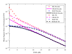
(a) i.i.d Gaussian channels

(b) Correlated non-zero mean channels

Figure 1: Average estimation square error compared with BCRLB/CRLB for ML and MAP estimation.

VI-B Acquisition Range and Combined Pilot Structure

Periodic and TD Pilots: Figure 2 shows the acquisition range of periodic and time division pilots at 20dB SNR. One can observe that the periodic pilot has smaller square error while the TD pilot has larger acquisition range that almost is the largest possible of $\left|\boldsymbol{f}_{\delta}-\mu_{\boldsymbol{f}_{\delta}}\right|<0.5$.

Combined Pilots: This observation motivates the combination of both pilot structure to design a pilot that has the advantages of both. Figure 3 shows that this is indeed possible. The combined pilot with 8 symbol time of periodic pilot followed by 8 symbol time of TD pilot achieves almost as small square error as the periodic pilot of the same length and almost as large acquisition range as the TD pilot of the same length.

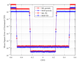
Figure 2: Acquisition range of CFO estimation for different pilots.

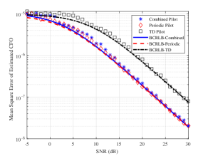
(a) Average square estimation errors and the BCRLB bounds

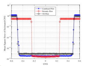
(b) Acquisition ranges

Figure 3: MSE and acquisition range of combined pilot comparing with the periodic and TD pilots

VI-C MAP Estimation for CFO Tracking

Tracking: The MAP estimation provides a means for tracking time varying parameters. Here, we give an example of CFO tracking by taking advantage of the prior knowledge, where the CFO changes from packet/frame to packet/frame but is correlated from frame to frame. The estimated CFO $\hat{f}_{\delta,\nu}$ of the $\nu$-th frame and its $\text{BCRLB}_{\nu}$ can be used together with the correlation model to calculate the $\nu+1$-th frame’s prior knowledge of $\boldsymbol{f}_{\delta,\nu+1}$. In this example, we assume the channel is independent from frame to frame to isolate the benefit of CFO tracking.

Example Model: We use a simple AR model for the CFO. It is straightforward for a designer to adapt the result here for other desired models. The model is $\boldsymbol{f}_{\delta,\nu+1}=\rho\boldsymbol{f}_{\delta,\nu}+(1-\rho)\mu_{\boldsymbol{f}_{\delta}}+\boldsymbol{w}_{\nu+1},$ where $0\leq\rho\leq 1$ controls the correlation; $\mu_{\boldsymbol{f}_{\delta}}$ is the stationary mean; and $\boldsymbol{w}_{\nu+1}\sim\mathcal{N}(0,\sigma_{\boldsymbol{w}}^{2})$ is an i.i.d. Gaussian noise. Since the MAP estimation approximately achieves BCRLB for almost all SNR according to the above simulation results, we may approximately assume $B_{\nu}=\left\{\boldsymbol{f}_{\delta,\nu}:\text{E}\left[\boldsymbol{f}_{\delta,\nu}\right]=\hat{f}_{\delta,\nu},\text{Var}\left[\boldsymbol{f}_{\delta,\nu}-\hat{f}_{\delta,\nu}\right]=\text{BCRLB}_{\nu}\right\}$ after finishing the estimation using frame $\nu$. Then according to the AR model, the conditional mean $\text{E}\left[\boldsymbol{f}_{\delta,\nu+1}|B_{\nu}\right]$ $=\rho\hat{f}_{\delta,\nu}+(1-\rho)\mu_{\boldsymbol{f}_{\delta}}$ and conditional variance $\text{Var}\left[\boldsymbol{f}_{\delta,\nu+1}|B_{\nu}\right]$ $=\rho^{2}\text{BCRLB}_{\nu}+\sigma_{w}^{2}$ may serve as the prior knowledge for frame $\nu+1$. The stationary variance is $\text{Var}\left[\boldsymbol{f}_{\delta,\infty}\right]$ $=\frac{\sigma_{w}^{2}}{1-\rho^{2}}$.

Observation: For the AR model with $\rho=0.9,\mu_{\boldsymbol{f}_{\delta}}=0.1,\sigma_{w}^{2}=10^{-8},$ $\text{SNR}=10\text{dB}$, and pilot length per frame $n=16$, the simulation result is in Figure 4. For the first frame, the variance of the CFO is assumed to be infinity, resulting in an ML estimation. The MAP estimation is applied since the 2nd frame. We can observe that the MAP tracking performance improves over time and is much better than the ML estimation that does not use the prior knowledge. The BCRLBs for periodic and TD pilot in the figure overlap in this case and assume perfect estimation of the previous frame. Thus, it is a lower bound. If desired, the performance can be improved by a backward belief propagation from the last frame to the first frame.

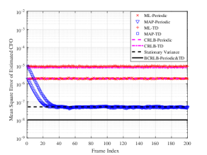
Figure 4: Tracking performance of CFO estimation in i.i.d channels

VII Conclusion

In this paper, the solution of the joint MAP estimation of channel states and the frequency offset is provided. Unexpectedly, the solution is separable with an individual MAP estimation of the CFO with channel statistic information first. An almost closed form algorithm is given. The Bayesian Cramér-Rao Lower bounds (BCRLB) is derived in closed form for the frequency offset estimation with prior knowledge. Based on it, pilot signal signal design guideline is provided on mean square error and acquisition range trade-off. Simulations with different pilot structures are conducted and analyzed. The simulation results show that the proposed algorithm has bound-approaching performance at almost all SNR and a wide acquisition range. The MAP estimation provides a different means to track time varying CFO, as demonstrated in simulation, and can achieve much better performance than the ML estimation.

Appendix A Proof of Theorem 3 of the MAP Estimator

Since $\det(\pi\Sigma_{\vec{\boldsymbol{y}}|\boldsymbol{f}_{\delta}})$ is not a function of $f_{\delta}$, we can maximize the exponent in (12) as

$$\hat{f}_{\delta} = \arg\max_{f_{\delta}}f_{\vec{\boldsymbol{y}}|\boldsymbol{f}_{\delta}}(\vec{y}|f_{\delta})f_{\boldsymbol{f}_{\delta}}(f_{\delta})$$ (36)

$$= \arg\max_{f_{\delta}}-\left(\vec{y}-\vec{\mu}_{\vec{\boldsymbol{y}}|\boldsymbol{f}_{\delta}}\right)^{\dagger}\Sigma_{\vec{\boldsymbol{y}}|\boldsymbol{f}_{\delta}}^{-1}\left(\vec{y}-\vec{\mu}_{\vec{\boldsymbol{y}}|\boldsymbol{f}_{\delta}}\right)$$

$$-\frac{1}{2}\sigma_{\boldsymbol{f}_{\delta}}^{-2}\left|f_{\delta}-\mu_{\boldsymbol{f}_{\delta}}\right|^{2}$$

We calculate the terms in (36) below. The conditional covariance

$$\Sigma_{\vec{\boldsymbol{y}}|\boldsymbol{f}_{\delta}}^{-1} = \left(\grave{X}\Sigma_{\vec{\boldsymbol{h}}}\grave{X}^{\dagger}+I\right)^{-1}$$

$$= \left(I-\grave{X}\left(\Sigma_{\vec{\boldsymbol{h}}}^{-1}+\grave{X}^{\dagger}\grave{X}\right)^{-1}\grave{X}^{\dagger}\right)$$

$$= \left(I-\grave{X}\left(\Sigma_{\vec{\boldsymbol{h}}}^{-1}+\grave{S}^{\dagger}\grave{S}\right)^{-1}\grave{X}^{\dagger}\right)$$

is converted by the Woodbury matrix identity. Then

$$\left(\vec{y}-\vec{\mu}_{\vec{\boldsymbol{y}}|\boldsymbol{f}_{\delta}}\right)^{\dagger}I\left(\vec{y}-\vec{\mu}_{\vec{\boldsymbol{y}}|\boldsymbol{f}_{\delta}}\right)$$ (38)

$$= \vec{y}^{\dagger}\vec{y}+\vec{\mu}_{\vec{\boldsymbol{y}}|\boldsymbol{f}_{\delta}}^{\dagger}\vec{\mu}_{\vec{\boldsymbol{y}}|\boldsymbol{f}_{\delta}}-2\Re\left[\left\langle\vec{y},\vec{\mu}_{\vec{\boldsymbol{y}}|\boldsymbol{f}_{\delta}}\right\rangle\right]$$

$$= \vec{y}^{\dagger}\vec{y}+\vec{\mu}_{\vec{\boldsymbol{h}}}^{\dagger}\grave{X}^{\dagger}\grave{X}\vec{\mu}_{\vec{\boldsymbol{h}}}-2\Re\left[\left\langle\vec{y},\grave{X}\vec{\mu}_{\vec{\boldsymbol{h}}}\right\rangle\right]$$

$$= \vec{y}^{\dagger}\vec{y}+\vec{\mu}_{\vec{\boldsymbol{h}}}^{\dagger}\grave{S}^{\dagger}\grave{S}\vec{\mu}_{\vec{\boldsymbol{h}}}-2\Re\left[\left\langle\grave{X}^{\dagger}\vec{y},\vec{\mu}_{\vec{\boldsymbol{h}}}\right\rangle\right],$$

and

$$\left(\vec{y}-\vec{\mu}_{\vec{\boldsymbol{y}}|\boldsymbol{f}_{\delta}}\right)^{\dagger}\grave{X}\left(\Sigma_{\vec{\boldsymbol{h}}}^{-1}+\grave{S}^{\dagger}\grave{S}\right)^{-1}\grave{X}^{\dagger}\left(\vec{y}-\vec{\mu}_{\vec{\boldsymbol{y}}|\boldsymbol{f}_{\delta}}\right)$$ (39)

$$= \left(\grave{X}^{\dagger}\vec{y}-\grave{S}^{\dagger}\grave{S}\vec{\mu}_{\vec{\boldsymbol{h}}}\right)^{\dagger}\left(\Sigma_{\vec{\boldsymbol{h}}}^{-1}+\grave{S}^{\dagger}\grave{S}\right)^{-1}\left(\grave{X}^{\dagger}\vec{y}-\grave{S}^{\dagger}\grave{S}\vec{\mu}_{\vec{\boldsymbol{h}}}\right)$$

$$= \left(\grave{X}^{\dagger}\vec{y}\right)^{\dagger}\left(\Sigma_{\vec{\boldsymbol{h}}}^{-1}+\grave{S}^{\dagger}\grave{S}\right)^{-1}\left(\grave{X}^{\dagger}\vec{y}\right)+$$

$$\left(\grave{S}^{\dagger}\grave{S}\vec{\mu}_{\vec{\boldsymbol{h}}}\right)^{\dagger}\left(\Sigma_{\vec{\boldsymbol{h}}}^{-1}+\grave{S}^{\dagger}\grave{S}\right)^{-1}\left(\grave{S}^{\dagger}\grave{S}\vec{\mu}_{\vec{\boldsymbol{h}}}\right)$$

$$-2\Re\left[\left(\grave{S}^{\dagger}\grave{S}\vec{\mu}_{\vec{\boldsymbol{h}}}\right)^{\dagger}\left(\Sigma_{\vec{\boldsymbol{h}}}^{-1}+\grave{S}^{\dagger}\grave{S}\right)^{-1}\left(\grave{X}^{\dagger}\vec{y}\right)\right].$$

After discarding terms in (38) and (39) that are not functions of $f_{\delta}$, we obtain (14).

Appendix B Proof of Theorem 6

We find the derivatives of the three terms in $\frac{\partial g(\vec{y},f_{\delta})}{\partial f_{\delta}}$ of (14) as follows. The first one is

$$\frac{\partial 2\Re\left[\left\langle\grave{X}^{\dagger}\vec{y},\vec{b}\right\rangle\right]}{\partial f_{\delta}}$$ (40)

$$= 2\Re\left[\left\langle\frac{\partial}{\partial f_{\delta}}\left[S^{\dagger}\left[e^{-j2\pi f_{\delta}(k-1)}y_{r,k}\right]_{k}\right]_{r},\vec{b}\right\rangle\right]$$

$$= 2\Re\left[-j2\pi\left\langle\left[S^{\dagger}\left[(k-1)e^{-j2\pi f_{\delta}(k-1)}y_{r,k}\right]_{k}\right]_{r},\vec{b}\right\rangle\right]$$

$$= 4\pi\Im\left[\left\langle\left[S^{\dagger}\left[(k-1)e^{-j2\pi f_{\delta}(k-1)}y_{r,k}\right]_{k}\right]_{r},\vec{b}\right\rangle\right]$$

$$= 4\pi\Im\left[\sum_{k^{\prime}=1}^{n-1}e^{-j2\pi f_{\delta}k^{\prime}}k^{\prime}\sum_{r,t}s_{t,k^{\prime}+1}^{*}y_{r,k^{\prime}+1}b_{r,t}^{*}\right]$$

$$= -4\pi\Im\left[\sum_{k^{\prime}=1}^{n-1}e^{j2\pi f_{\delta}k^{\prime}}k^{\prime}\sum_{r,t}s_{t,k^{\prime}+1}y_{r,k^{\prime}+1}^{*}b_{r,t}\right].$$

The second one is

$$\frac{\partial\left(\grave{X}^{\dagger}\vec{y}\right)^{\dagger}A\left(\grave{X}^{\dagger}\vec{y}\right)}{\partial f_{\delta}}$$ (42)

$$= \frac{\partial\text{Tr}\left(A\left(\grave{X}^{\dagger}\vec{y}\right)\left(\grave{X}^{\dagger}\vec{y}\right)^{\dagger}\right)}{\partial f_{\delta}}$$

$$= \frac{\partial\text{Tr}\left(A\grave{S}^{\dagger}\grave{F}^{\dagger}\vec{y}\vec{y}^{\dagger}\grave{F}\grave{S}\right)}{\partial f_{\delta}}$$

$$= \text{Tr}\left(A\grave{S}^{\dagger}\left[\left[\frac{\partial}{\partial f_{\delta}}e^{j2\pi f_{\delta}(k_{1}-k_{2})}\right.\right.\right.$$

$$\left.\left.\left.\times y_{r_{2},k_{2}}y_{r_{1},k_{1}}^{*}\right]_{k_{2},k_{1}}\right]_{r_{2},r_{1}}\grave{S}\right)$$

$$= \text{Tr}\left(A\left[S^{\dagger}\left[j2\pi(k_{1}-k_{2})e^{j2\pi f_{\delta}(k_{1}-k_{2})}\right.\right.\right.$$

$$\left.\left.\left.\times y_{r_{2},k_{2}}y_{r_{1},k_{1}}^{*}\right]_{k_{2},k_{1}}S\right]_{r_{2},r_{1}}\right)$$

$$= j2\pi\sum_{k_{1},k_{2}}e^{j2\pi f_{\delta}(k_{1}-k_{2})}(k_{1}-k_{2})\times$$

$$\sum_{r_{1},t_{1},r_{2},t_{2}}s_{t_{1},k_{1}}a_{r_{1},t_{1},r_{2},t_{2}}s_{t_{2},k_{2}}^{*}y_{r_{2},k_{2}}y_{r_{1},k_{1}}^{*}$$

$$= -4\pi\Im\left[\sum_{k^{\prime}=1}^{n-1}e^{j2\pi f_{\delta}k^{\prime}}k^{\prime}\sum_{k_{1}=k^{\prime}+1}^{n}\sum_{r_{1},t_{1},r_{2},t_{2}}\right.$$

$$\left.a_{r_{1},t_{1},r_{2},t_{2}}s_{t_{1},k_{1}}s_{t_{2},k_{1}-k^{\prime}}^{*}y_{r_{2},k_{1}-k^{\prime}}y_{r_{1},k_{1}}^{*}\right],$$

where (42) follows from the observation that $x-x^{*}=2j\Im[x]$ and that the summand in (42) is anti-symmetric when exchanging $k_{1}$ and $k_{2}$ and thus, we only need to sum for $k_{1}>k_{2}$, while defining $k^{\prime}=k_{1}-k_{2}$ and replacing $k_{2}=k_{1}-k^{\prime}$. The third one is

$$-\frac{1}{2}\sigma_{\boldsymbol{f}_{\delta}}^{-2}\frac{\partial}{\partial f_{\delta}}\left|f_{\delta}-\mu_{\boldsymbol{f}_{\delta}}\right|^{2}$$ (43)

$$= -\sigma_{\boldsymbol{f}_{\delta}}^{-2}\left(f_{\delta}-\mu_{\boldsymbol{f}_{\delta}}\right).$$

Combing eq. (40, 42, 43), we obtain eq. (15, 16).

Appendix C Proof of Theorem 12 of the Cramer-Rao Lower Bound

To calculate the BCRLB, calculate

$$\frac{\partial^{2}\ln\left(f_{\vec{\boldsymbol{y}}|\boldsymbol{f}_{\delta}}(\vec{y}|f_{\delta})f_{\boldsymbol{f}_{\delta}}(f_{\delta})\right)}{\partial f_{\delta}^{2}}$$

$$= \frac{\partial^{2}g(\vec{y},f_{\delta})}{\partial f_{\delta}^{2}}$$

$$= -\frac{\partial}{\partial f_{\delta}}4\pi\Im\left[\sum_{k=1}^{n-1}e^{j2\pi f_{\delta}k}kr_{k}e^{-j\theta_{k}}\right]$$

$$-\frac{\partial}{\partial f_{\delta}}\sigma_{\boldsymbol{f}_{\delta}}^{-2}\left(f_{\delta}-\mu_{\boldsymbol{f}_{\delta}}\right)$$

$$= -4\pi\Im\left[j2\pi\sum_{k=1}^{n-1}e^{j2\pi f_{\delta}k}k^{2}r_{k}e^{-j\theta_{k}}\right]-\sigma_{\boldsymbol{f}_{\delta}}^{-2}$$

$$= -8\pi^{2}\Re\left[\sum_{k=1}^{n-1}e^{j2\pi f_{\delta}k}k^{2}r_{k}e^{-j\theta_{k}}\right]-\sigma_{\boldsymbol{f}_{\delta}}^{-2},$$

where we have used (15).

Note that $\text{E}\left[\cdot\right]=\text{E}_{\boldsymbol{f}_{\delta}}\left[\text{E}_{\vec{\boldsymbol{y}}|\boldsymbol{f}_{\delta}}\left[\cdot\right]\right]$. We calculate

$$\text{E}_{\vec{\boldsymbol{y}}|\boldsymbol{f}_{\delta}}\left[\frac{\partial^{2}\ln\left(f_{\vec{\boldsymbol{y}}|\boldsymbol{f}_{\delta}}(\vec{\boldsymbol{y}}|\boldsymbol{f}_{\delta})f_{\boldsymbol{f}_{\delta}}(\boldsymbol{f}_{\delta})\right)}{\partial\boldsymbol{f}_{\delta}^{2}}\right]$$ (45)

$$= -8\pi^{2}\Re\left[\sum_{k=1}^{n-1}e^{j2\pi\boldsymbol{f}_{\delta}k}k^{2}\text{E}_{\vec{\boldsymbol{y}}|\boldsymbol{f}_{\delta}}\left[\boldsymbol{r}_{k}e^{-j\boldsymbol{\theta}_{k}}\right]\right]-\sigma_{\boldsymbol{f}_{\delta}}^{-2}$$

first. Inspecting (16), we need to calculate

$$\text{E}_{\vec{\boldsymbol{y}}|\boldsymbol{f}_{\delta}}\left[\boldsymbol{y}_{r,k+1}^{*}\right]$$

$$= \text{E}_{\vec{\boldsymbol{y}}|\boldsymbol{f}_{\delta}}\left[e^{-j2\pi\boldsymbol{f}_{\delta}k}\sum_{t^{\prime}}s_{t^{\prime},k+1}^{*}\boldsymbol{h}_{r,t^{\prime}}^{*}+\boldsymbol{n}_{r,k+1}^{*}\right]$$

$$= e^{-j2\pi\boldsymbol{f}_{\delta}k}\sum_{t^{\prime}}s_{t^{\prime},k+1}^{*}\mu_{\boldsymbol{h}_{r,t^{\prime}}}^{*}$$

and

$$\text{E}_{\vec{\boldsymbol{y}}|\boldsymbol{f}_{\delta}}\left[y_{r_{1},k_{1}}^{*}y_{r_{2},k_{2}}\right]$$

$$= \text{E}_{\vec{\boldsymbol{y}}|\boldsymbol{f}_{\delta}}\left[\left(e^{-j2\pi\boldsymbol{f}_{\delta}(k_{1}-1)}\sum_{t_{1}^{\prime}}s_{t_{1}^{\prime},k_{1}}^{*}\boldsymbol{h}_{r_{1},t_{1}^{\prime}}^{*}+\boldsymbol{n}_{r_{1},k_{1}}^{*}\right)\right.$$

$$\left.\left(e^{j2\pi\boldsymbol{f}_{\delta}(k_{2}-1)}\sum_{t_{2}^{\prime}}s_{t_{2}^{\prime},k_{2}}\boldsymbol{h}_{r_{2},t_{2}^{\prime}}+\boldsymbol{n}_{r_{2},k_{2}}\right)\right]$$

$$\stackrel{{\scriptstyle k_{2}=k_{1}-k}}{{=}} e^{-j2\pi\boldsymbol{f}_{\delta}k}\sum_{t_{1}^{\prime}}s_{t_{1}^{\prime},k_{1}}^{*}\sum_{t_{2}^{\prime}}s_{t_{2}^{\prime},k_{1}-k}\text{E}\left[\boldsymbol{h}_{r_{1},t_{1}^{\prime}}^{*}\boldsymbol{h}_{r_{2},t_{2}^{\prime}}\right]$$

$$+\delta[r_{1}-r_{2}]\delta[k],$$

where $\text{E}\left[\boldsymbol{h}_{r_{1},t_{1}^{\prime}}^{*}\boldsymbol{h}_{r_{2},t_{2}^{\prime}}\right]=c_{\boldsymbol{h}_{r_{1},t_{1}^{\prime}}\boldsymbol{h}_{r_{2},t_{2}^{\prime}}}^{*}+\mu_{\boldsymbol{h}_{r_{2},t_{2}^{\prime}}}\mu_{\boldsymbol{h}_{r_{1},t_{1}^{\prime}}}^{*}$; and $c_{\boldsymbol{h}_{r_{1},t_{1}^{\prime}}\boldsymbol{h}_{r_{2},t_{2}^{\prime}}}$ is defined in (4). They are used to obtain

$$\text{E}_{\vec{\boldsymbol{y}}|\boldsymbol{f}_{\delta}}\left[\boldsymbol{r}_{k}e^{-j\boldsymbol{\theta}_{k}}\right]$$ (46)

$$= e^{-j2\pi\boldsymbol{f}_{\delta}k}\sum_{r,t}\sum_{t^{\prime}}s_{t,k+1}s_{t^{\prime},k+1}^{*}\mu_{\boldsymbol{h}_{r,t^{\prime}}}^{*}b_{r,t}+$$

$$e^{-j2\pi\boldsymbol{f}_{\delta}k}\sum_{k_{1}=k+1}^{n}\sum_{r_{1},t_{1},r_{2},t_{2}}a_{r_{1},t_{1},r_{2},t_{2}}\times$$

$$s_{t_{1},k_{1}}s_{t_{2},k_{1}-k}^{*}\sum_{t_{2}^{\prime}}s_{t_{2}^{\prime},k_{1}-k}\sum_{t_{1}^{\prime}}s_{t_{1}^{\prime},k_{1}}^{*}\times$$

$$\left(c_{\boldsymbol{h}_{r_{1},t_{1}^{\prime}},\boldsymbol{h}_{r_{2},t_{2}^{\prime}}}^{*}+\mu_{\boldsymbol{h}_{r_{2},t_{2}^{\prime}}}\mu_{\boldsymbol{h}_{r_{1},t_{1}^{\prime}}}^{*}\right),\ k\neq 0.$$

Plug (46) into (45), we see that $\text{E}_{\vec{\boldsymbol{y}}|\boldsymbol{f}_{\delta}}\left[\frac{\partial^{2}\ln\left(f_{\vec{\boldsymbol{y}}|\boldsymbol{f}_{\delta}}(\vec{\boldsymbol{y}}|\boldsymbol{f}_{\delta})f_{\boldsymbol{f}_{\delta}}(\boldsymbol{f}_{\delta})\right)}{\partial\boldsymbol{f}_{\delta}^{2}}\right]$ is not a function of $\boldsymbol{f}_{\delta}$. Therefore,

$$\text{E}_{\vec{\boldsymbol{y}}|\boldsymbol{f}_{\delta}}\left[\frac{\partial^{2}\ln\left(f_{\vec{\boldsymbol{y}}|\boldsymbol{f}_{\delta}}(\vec{\boldsymbol{y}}|\boldsymbol{f}_{\delta})f_{\boldsymbol{f}_{\delta}}(\boldsymbol{f}_{\delta})\right)}{\partial\boldsymbol{f}_{\delta}^{2}}\right]$$

$$= \text{E}_{\boldsymbol{f}_{\delta}}\left[\text{E}_{\vec{\boldsymbol{y}}|\boldsymbol{f}_{\delta}}\left[\frac{\partial^{2}\ln\left(f_{\vec{\boldsymbol{y}}|\boldsymbol{f}_{\delta}}(\vec{\boldsymbol{y}}|\boldsymbol{f}_{\delta})f_{\boldsymbol{f}_{\delta}}(\boldsymbol{f}_{\delta})\right)}{\partial\boldsymbol{f}_{\delta}^{2}}\right]\right],$$

which is plugged into (29) to obtain $\beta$ of BCRLB in (32).

One can calculate $\text{E}_{\vec{\boldsymbol{y}}|\{\boldsymbol{f}_{\delta}=f_{\delta}\}}\left[\frac{\partial^{2}\ln\left(f_{\vec{\boldsymbol{y}}|\boldsymbol{f}_{\delta}}(\vec{\boldsymbol{y}}|f_{\delta})\right)}{\partial f_{\delta}^{2}}\right]$ and observe that it is obtained by setting $\sigma_{\boldsymbol{f}_{\delta}}^{-2}=0$. This gives CRLB.

• For i.i.d. zero mean channel, (33) is proved by plugging (18) into (32) and employing the definition of $\ddot{s}_{k_{1},k_{1}-k}$ in (20).

  • For periodic pilot, observe that according to 20,

    $$\left|\ddot{s}_{k_{1},k_{1}-k}\right|^{2} = \rho^{2}$$

    is only nonzero for $k=il_{\text{t}}$, $i=1,...,m-1$. Define $k_{1}=(i_{1}-1)l_{\text{t}}+i_{2}$, $i_{1}=i+1,...,m$, $i_{2}=1,...,l_{\text{t}}$. Then in 33,

    $$\sum_{k=1}^{n-1}k^{2}\sum_{k_{1}=k+1}^{n}\left|\ddot{s}_{k_{1},k_{1}-k}\right|^{2}$$

    $$= \sum_{i=1}^{m-1}(il_{\text{t}})^{2}\sum_{i_{1}=i+1}^{m}\sum_{i_{2}=1}^{l_{\text{t}}}\rho^{2}$$

    $$= \rho^{2}l_{\text{t}}^{3}\sum_{i=1}^{m-1}i^{2}(m-i)$$

    $$= \rho^{2}l_{\text{t}}^{3}\left(\frac{m(m-1)m(2m-1)}{6}-\frac{(m-1)^{2}m^{2}}{4}\right)$$

    $$= \rho^{2}l_{\text{t}}^{3}\left(\frac{m^{2}(m^{2}-1)}{12}\right).$$

    $$= \frac{\rho^{2}}{l_{\text{t}}}\left(\frac{n^{2}(n^{2}-l_{\text{t}}^{2})}{12}\right),$$

    which produces 34.

  • For time division pilot, observe that according to 20,

    $$\left|\ddot{s}_{k_{1},k_{1}-k}\right|^{2} = \rho^{2}$$

    is only nonzero for $k=i=1,...,m-1$. Define $k_{1}=(i_{2}-1)m+i_{1}$, $i_{2}=1,...,l_{\text{t}}$, $i_{1}=i+1,...,m$. Then in 33, similarly

    $$\sum_{k=1}^{n-1}k^{2}\sum_{k_{1}=k+1}^{n}\left|\ddot{s}_{k_{1},k_{1}-k}\right|^{2}$$

    $$= \sum_{i=1}^{m-1}(i)^{2}\sum_{i_{1}=i+1}^{m}\sum_{i_{2}=1}^{l_{\text{t}}}\rho^{2}$$

    $$= \frac{\rho^{2}}{l_{\text{t}}^{3}}\left(\frac{n^{2}(n^{2}-l_{\text{t}}^{2})}{12}\right),$$

    which produces 34.

References

• [1] O. Besson and P. Stoica, “On parameter estimation of MIMO flat-fading channels with frequency offsets,” IEEE Transactions on Signal Processing, vol. 51, no. 3, pp. 602–613, 2003. [Online]. Available: http://ieeexplore.ieee.org/abstract/document/1179750/
• [2] D. Rife and R. Boorstyn, “Single tone parameter estimation from discrete-time observations,” IEEE Transactions on Information Theory, vol. 20, no. 5, pp. 591–598, Sep. 1974.
• [3] M. Luise and R. Reggiannini, “Carrier frequency recovery in all-digital modems for burst-mode transmissions,” IEEE Transactions on Communications, vol. 43, no. 2, 3, 4, pp. 1169–1178, 1995. [Online]. Available: http://ieeexplore.ieee.org/abstract/document/380149/
• [4] W.-Y. Kuo and M. P. Fitz, “Frequency offset compensation of pilot symbol assisted modulation in frequency flat fading,” IEEE Transactions on Communications, vol. 45, no. 11, pp. 1412–1416, Nov. 1997.
• [5] M. Morelli, U. Mengali, and G. M. Vitetta, “Further results in carrier frequency estimation for transmissions over flat fading channels,” IEEE Communications Letters, vol. 2, no. 12, pp. 327–330, Dec. 1998.
• [6] O. Besson and P. Stoica, “On frequency offset estimation for flat-fading channels,” IEEE Communications Letters, vol. 5, no. 10, pp. 402–404, Oct. 2001.
• [7] F. Simoens and M. Moeneclaey, “Reduced complexity data-aided and code-aided frequency offset estimation for flat-fading MIMO channels,” IEEE Transactions on Wireless Communications, vol. 5, no. 6, pp. 1558–1567, Jun. 2006.
• [8] T. H. Pham, A. Nallanathan, and Y. C. Liang, “Joint channel and frequency offset estimation in distributed MIMO flat-fading channels,” IEEE Transactions on Wireless Communications, vol. 7, no. 2, pp. 648–656, Feb. 2008.
• [9] P. A. Parker, P. Mitran, D. W. Bliss, and V. Tarokh, “On Bounds and Algorithms for Frequency Synchronization for Collaborative Communication Systems,” IEEE Transactions on Signal Processing, vol. 56, no. 8, pp. 3742–3752, Aug. 2008.
• [10] A. N. Mody and G. L. Stuber, “Synchronization for MIMO OFDM systems,” in IEEE Global Telecommunications Conference, 2001. GLOBECOM ’01, vol. 1, 2001, pp. 509–513 vol.1.
• [11] Y. Zeng and T.-S. Ng, “A semi-blind channel estimation method for multiuser multiantenna OFDM systems,” IEEE Transactions on Signal Processing, vol. 52, no. 5, pp. 1419–1429, 2004.
• [12] Y. Sun, Z. Xiong, and X. Wang, “EM-based iterative receiver design with carrier-frequency offset estimation for MIMO OFDM systems,” IEEE Transactions on Communications, vol. 53, no. 4, pp. 581–586, Apr. 2005.
• [13] M. O. Pun, M. Morelli, and C. C. J. Kuo, “Maximum-likelihood synchronization and channel estimation for OFDMA uplink transmissions,” IEEE Transactions on Communications, vol. 54, no. 4, pp. 726–736, Apr. 2006.
• [14] H. Minn, N. Al-Dhahir, and Y. Li, “Optimal training signals for MIMO OFDM channel estimation in the presence of frequency offset and phase noise,” IEEE Transactions on Communications, vol. 54, no. 10, pp. 1754–1759, Oct. 2006.
• [15] Y. Zeng, A. R. Leyman, and T.-S. Ng, “Joint semiblind frequency offset and channel estimation for multiuser MIMO-OFDM uplink,” IEEE Transactions on Communications, vol. 55, no. 12, pp. 2270–2278, 2007.
• [16] H. Nguyen-Le, T. Le-Ngoc, and C. C. Ko, “Joint Channel Estimation and Synchronization for MIMO-OFDM in the Presence of Carrier and Sampling Frequency Offsets,” IEEE Transactions on Vehicular Technology, vol. 58, no. 6, pp. 3075–3081, Jul. 2009.
• [17] E. P. Simon, L. Ros, H. Hijazi, J. Fang, D. P. Gaillot, and M. Berbineau, “Joint Carrier Frequency Offset and Fast Time-Varying Channel Estimation for MIMO-OFDM Systems,” IEEE Transactions on Vehicular Technology, vol. 60, no. 3, pp. 955–965, Mar. 2011.
• [18] R. Jose and K. Hari, “Joint estimation of synchronization impairments in MIMO-OFDM system,” in Communications (NCC), 2012 National Conference On.   IEEE, 2012, pp. 1–5.
• [19] M. Morelli and M. Moretti, “Joint maximum likelihood estimation of CFO, noise power, and SNR in OFDM systems,” IEEE Wireless Communications Letters, vol. 2, no. 1, pp. 42–45, 2013.
• [20] H. Solis-Estrella and A. G. Orozco-Lugo, “Carrier frequency offset estimation in OFDMA using digital filtering,” IEEE Wireless Communications Letters, vol. 2, no. 2, pp. 199–202, 2013.
• [21] W. Zhang, Q. Yin, and F. Gao, “Computationally Efficient Blind Estimation of Carrier Frequency Offset for MIMO-OFDM Systems,” IEEE Transactions on Wireless Communications, vol. 15, no. 11, pp. 7644–7656, Nov. 2016.
• [22] A. A. Nasir, S. Durrani, and R. A. Kennedy, “Blind timing and carrier synchronisation in distributed multiple input multiple output communication systems,” IET communications, vol. 5, no. 7, pp. 1028–1037, 2011. [Online]. Available: http://digital-library.theiet.org/content/journals/10.1049/iet-com.2010.0528
• [23] N. Shah, M. Ghosh, P. Xia, Z. You, F. La Sita, R. Olesen, and O. Oteri, “Carrier frequency offset correction for uplink multi-user MIMO for next generation Wi-Fi,” in Computing, Networking and Communications (ICNC), 2015 International Conference On.   IEEE, 2015, pp. 1004–1008.
• [24] H. Mehrpouyan and S. D. Blostein, “Bounds and Algorithms for Multiple Frequency Offset Estimation in Cooperative Networks,” IEEE Transactions on Wireless Communications, vol. 10, no. 4, pp. 1300–1311, Apr. 2011.
• [25] D. Chu, “Polyphase codes with good periodic correlation properties (Corresp.),” IEEE Transactions on Information Theory, vol. 18, no. 4, pp. 531–532, Jul. 1972.
• [26] H. L. V. Trees, K. L. Bell, and Z. Tian, Detection Estimation and Modulation Theory, Part I: Detection, Estimation, and Filtering Theory, 2nd ed.   Hoboken, N.J: Wiley, Apr. 2013.