Scaling of diffraction intensities near the origin:
Some rigorous results

Abstract.

The scaling behaviour of the diffraction intensity near the origin is investigated for (partially) ordered systems, with an emphasis on illustrative, rigorous results. This is an established method to detect and quantify the fluctuation behaviour known under the term hyperuniformity. Here, we consider one-dimensional systems with pure point, singular continuous and absolutely continuous diffraction spectra, which include perfectly ordered cut and project and inflation point sets as well as systems with stochastic disorder.

1. Introduction

While the concept of order is intuitive, it is surprisingly challenging to ‘measure’ the order in a system in a way that leads to a meaningful classification of different manifestations of order in Nature. Some of the most prominent measures available are based on ideas from statistical physics and crystallography, such as entropy which is closely related to disorder, or diffraction which is the main tool for determining the structure of solids. Essentially, diffraction is the Fourier transform of the pair correlation function, and hence quantifies the order in the two-point correlations of the structure.

Following the discovery of quasicrystals in the early 1980s, a proper mathematical treatment of the diffraction of aperiodically ordered structures was required; see [11, 28] and references therein for background and details. It turns out that there is a close connection between diffraction and what is known as the dynamical spectrum in mathematics [16]. The latter is the spectrum of the corresponding Koopman operator and is an important concept in ergodic theory. Aperiodically ordered structures, in particular those constructed by inflation rules, provide interesting examples of systems that exhibit a scaling (self-similarity) type of order, which differs substantially from the translational order found in periodic structures, such as conventional crystals.

Starting from the idea to use the degree of ‘(hyper)uniformity’ in density fluctuations in many-particle systems [39] to characterise their order, the scaling behaviour of the diffraction near the origin has emerged as a measure that captures the variance of the long-distance correlations. Recently, a number of conjectures on the scaling behaviour of the diffraction of aperiodically ordered structures were made [34, 35], reformulating and extending earlier, partly heuristic, results by Luck [31] from this perspective; see also [3, 27].

The purpose of this article is to link the recent interest in these questions with some of the known techniques and results from rigorous diffraction theory, as started by Hof in [28] and later developed by many people; see [11] and references therein for a systematic account. Our approach will make substantial use of the exact renormalisation relations for primitive inflation rules [5, 6, 8, 32, 13], which will allow us to establish the scaling behaviour rigorously. This is in some contrast to classic methods of finite size scaling [1, 24, 23, 2], where such a behaviour is extrapolated and only asymptotically true.

The paper is organised as follows. We begin by recalling some background material on diffraction, the projection formalism, inflation rules and Lyapunov exponents in Section 2. Then, in Section 3, we discuss systems with pure point spectrum, starting from the paradigmatic Fibonacci chain, which we treat in two different ways. We also discuss various generalisations, including noble means inflations and a limit-periodic system. After a brief look into substitutions with more than two letters, we close with an instructive example of number-theoretic origin, which can also be understood as a projection set.

In Section 4, we summarise the situation for systems with absolutely continuous spectrum via a comparative exposition of random and deterministic cases. In particular, we discuss the Poisson process in comparison to the Rudin–Shapiro sequence, the classical random matrix ensembles, as well as the Markov lattice gas and binary random tilings. Finally, Section 5 deals with systems with singular continuous spectrum, of which the classic Thue –Morse sequence is a paradigm with a decay behaviour faster than any power law. We then embed this into the family of generalised Thue –Morse sequences.

2. Preliminaries and general methods

Our approach to the scaling behaviour of the diffraction measure near the origin requires a number of different methods. In this section, we summarise key results and provide references for background and further details.

2.1. Diffraction and scaling

Throughout this article, we use the notation and results from [11] on diffraction theory, as well as some more advanced results on the Fourier transform of measures from [33, 12]. Various definitions are discussed there, and we use standard results from these sources without further reference. Note that the term ‘measure’ in this context refers to general (complex) Radon measures in the mathematical sense. They can be identified with the continuous linear functionals on the space of compactly supported continuous functions on $\mathbb{R}^{d}$. In particular, given a (usually translation bounded) measure $\omega$, we assume that an averaging sequence $\mathcal{A}$ of van Hove type is specified, and the autocorrelation $\gamma=\gamma_{\omega}=\omega\circledast\widetilde{\omega}$ is given as the Eberlein (or volume-averaged) convolution along $\mathcal{A}$. The measure $\gamma$ is positive definite, and hence Fourier transformable as a measure.

The Fourier transform of $\gamma$ is the diffraction measure $\widehat{\gamma}$, which is a positive measure. This is the measure-theoretic formulation of the structure factor from physics and crystallography, which is better suited for rigorous results. In particular, this approach defines the different spectral components by means of the Lebesgue decomposition

$$\widehat{\gamma}\,=\,\widehat{\gamma}_{\mathsf{pp}}+\widehat{\gamma}_{\mathsf{sc}}+\widehat{\gamma}_{\mathsf{ac}}$$

of $\widehat{\gamma}$ into its pure point, singular continuous and absolutely continuous parts; see [11, Sec. 8.5.2] for details. In what follows, we only consider the one-dimensional case.

For the investigation of scaling properties, we follow the existing literature and define

(1) $$Z(k)\,\mathrel{\mathop{:}}=\,\widehat{\gamma}\bigl{(}(0,k]\bigr{)},$$

which is a modified version of the distribution function of the diffraction measure. Due to the reflection symmetry of $\widehat{\gamma}$ with respect to the origin, this quantity can also be expressed as

$$Z(k)\,=\,\frac{\raisebox{-2.0pt}{$1$}}{\raisebox{0.5pt}{$2$}}\Bigl{(}\widehat{\gamma}\bigl{(}[-k,k]\bigr{)}-\widehat{\gamma}\bigl{(}\{0\}\bigr{)}\Bigr{)}.$$

Sometimes, it is natural to replace $Z(k)$ by $Z(k)/I(0)$, where $I(0)=\widehat{\gamma}\bigl{(}\{0\}\bigr{)}$ is the intensity of the central diffraction (or Bragg) peak. Note that this just amounts to a different normalisation. It will always be clear from the context when we do so. This normalisation has no influence on the scaling behaviour of $Z(k)$ as $k\,\raisebox{2.0pt}{$\scriptscriptstyle\searrow$}\,0$.

The interest in the scaling near the origin is based on the intuition that the small-$k$ behaviour of the diffraction measure probes the long-wavelength fluctuations in the structure, which is related to the variance in the distribution of patches, and hence can serve as an indicator for the degree of uniformity of the structure [39]. Clearly, any periodic structure leads to $Z(k)=0$ for all sufficiently small $k$, so that the main interest is focused on non-periodic systems, both ordered and disordered.

2.2. Projection formalism

One way to produce well-ordered aperiodic systems is based on the (partial) projection of higher-dimensional (periodic) lattices. Such cut and project sets or model sets can be viewed as a generalised variant of the notion of a quasiperiodic function. We can only present a brief summary here, for details we refer to [11, Ch. 7]. The general setting for a model set in physical (direct) space $\mathbb{R}^{d}$ is encoded in the cut and project scheme (CPS) $(\mathbb{R}^{d},H,\mathcal{L})$,

(2) $$\begin{array}[]{r@{}ccccc@{}l}&\mathbb{R}^{d}&\xleftarrow{\,\;\;\pi\;\;\,}&\mathbb{R}^{d}\,\times\,H&\xrightarrow{\;\pi_{\mathrm{int}\;}}&H&\\ &\cup&&\cup&&\cup&\raisebox{1.0pt}{\text{\footnotesize dense}}\\ &\pi(\mathcal{L})&\xleftarrow{\;1-1\;}&\mathcal{L}&\xrightarrow{\;\hphantom{1-1}\;}&\pi_{\mathrm{int}}(\mathcal{L})&\\ &\|&&&&\|&\\ &L&\lx@intercol\hfil\xrightarrow{\qquad\quad\quad\;\;\;\star\;\;\;\quad\quad\qquad}\hfil\lx@intercol&{L}^{\star}&\\ \end{array}$$

where the internal space $H$ is a locally compact Abelian group (in many examples, $H$ will turn out to be another Euclidean space, so $H=\mathbb{R}^{m}$), $\mathcal{L}$ is a lattice (co-compact discrete subgroup) in $\mathbb{R}^{d}\times H$, and where $\pi$ and $\pi_{\mathrm{int}}$ denote the natural projections onto the physical and internal spaces. The assumption that $L=\pi(\mathcal{L})\subset\mathbb{R}^{d}$ is a bijective image of $\mathcal{L}$ in physical space guarantees that the $\star\,$-map $x\mapsto x^{\star}$ is well defined on $L$.

A model set for a given CPS is then a set of the form

(3) $$\varLambda\,=\,\mbox{\Large$\curlywedge$}(W)\,=\,\bigl{\{}x\in L:x^{\star}\in W\bigr{\}},$$

where the domain $W\subseteq H$ (called the window or acceptance domain) is a relatively compact set with non-empty interior. These conditions on the window guarantee that the model set $\varLambda\subseteq L$ is both uniformly discrete and relatively dense, so a Delone set in $\mathbb{R}^{d}$. If the window is sufficiently ‘nice’ (for instance, when $W$ is compact with boundary of measure $0$), the diffraction measure $\widehat{\gamma}$ of the associated Dirac comb

$$\delta_{\!\varLambda}\,\mathrel{\mathop{:}}=\sum_{x\in\varLambda}\delta_{x}$$

is a pure point measure; see [11, Ch. 9] for details. Note that the dynamical spectrum is pure point as well; see [16] and references therein.

Example 2.1.

Consider a CPS with $d=1$ and $H=\mathbb{R}$, and the planar lattice

$$\mathcal{L}\,=\,\bigg{\langle}\!\binom{1}{1},\binom{\tau}{1-\tau}\!\bigg{\rangle}_{\!\!\mathbb{Z}\hskip 0.5pt}\subset\,\mathbb{R}^{2},$$

where $\tau=\bigl{(}1+\sqrt{5}\,\bigr{)}/2$ is the golden ratio. The projection of $\mathcal{L}$ to physical space is the $\mathbb{Z}\hskip 0.5pt$-module $L=\mathbb{Z}\hskip 0.5pt[\tau]=\{m+n\tau\mid m,n\in\mathbb{Z}\hskip 0.5pt\}$, and similarly $L^{\star}=\mathbb{Z}\hskip 0.5pt[\tau]$. The $\star$-map acts as algebraic conjugation $\sqrt{5}\mapsto-\sqrt{5}$, so that $(m+n\tau)^{\star}=m+n-n\tau$. The Fibonacci model set is $\varLambda=\mbox{\Large$\curlywedge$}(W)$ with window $W=(-1,\tau-1]$. As indicated in Figure 1, the two different point types (left endpoints of long and short intervals, respectively) in the Fibonacci model set are obtained as model sets for the two smaller windows $W_{\!L}=(-1,\tau-2]$ and $W_{\!S}=(\tau-2,\tau-1]$, with $W=W_{\!L}\operatorname{\dot{\cup}}W_{\!S}$. $\Diamond$

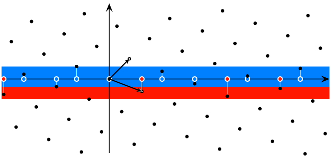
Figure 1. Projection description of the Fibonacci model set from Example 2.1. The horizontal line represents the physical space, the vertical line the internal space. The black points form the lattice $\mathcal{L}$. Points inside the strip $\mathbb{R}\times W$ are projected to physical space to produce the model set $\varLambda$.

2.3. Inflation rules and exact renormalisation

Another important construction of aperiodic sequences and tilings is based on substitution and inflation rules; see [11, Chs. 4–5] for background. The idea is perhaps most easily phrased in terms of tilings. Starting from a (finite) set of prototiles (equivalence classes of tiles under translation), an inflation rule consists of a rescaling (more generally, an expansive linear transformation) of the prototiles and a subsequent dissection of the rescaled tiles into prototiles of the original shape and size. Iterating such an inflation rule produces tilings of space, which generically will not be periodic. Let us illustrate this with the example of the Fibonacci model set from above, which can also be constructed by an inflation rule (note that this is not generally the case: Cut and project tilings generically do not possess an inflation symmetry, and inflation tilings generally do not allow an embedding into a higher-dimensional lattice with a bounded window).

Example 2.2.

Consider two prototiles (intervals) in $\mathbb{R}$, a long interval $a$ of length $\tau$ and a short interval $b$ of length $1$. The (geometric) Fibonacci inflation rule with inflation factor $\tau$ is

Starting from an initial configuration of, say, two adjacent large tiles with common vertex at the origin, and iterating this rule produces a tiling of $\mathbb{R}$ which is a fixed point under the square of the inflation rule. Denoting the set of left endpoints of intervals of type $a$ by $\varLambda_{a}$ and of type $b$ by $\varLambda_{b}$, we have $\varLambda_{a,b}\subset\mathbb{Z}\hskip 0.5pt[\tau]$ by construction, which are model sets in the description of Example 2.1; see [11, Ex. 7.3] for details. $\Diamond$

The inherent recursive structure of the inflation approach not only leads to recursive relations for the point sets constructed in this way, but also ensures the existence of a set of renormalisation equations for their two-point correlation functions; see [6] and references therein for details. Here, we illustrate this for the Fibonacci case.

Example 2.3.

Consider the point set $\varLambda=\varLambda_{a}\operatorname{\dot{\cup}}\varLambda_{b}$ constructed by the inflation of Example 2.2. Define the pair correlation functions (or coefficients) $\nu_{ij}(z)$ with $i,j\in\{a,b\}$ as the relative frequency (frequency per point of $\varLambda$) of two points in $\varLambda$ at distance $z$, subject to the condition that the left point is of type $i$ and the right point of type $j$. The pair correlation functions exist (as a consequence of unique ergodicity) and satisfy the relations $\nu_{ij}(z)=0$ for any $z\not\in\varLambda-\varLambda$, $\nu_{ij}(0)=0$ for $i\neq j$, and $\nu_{ij}(-z)=\nu_{ji}(z)$ for any $z$.

The recognisability of our inflation rule then implies the following set of exact renormalisation equations [6, 32, 8],

(4) $$\begin{split}\nu_{aa}(z)\,&=\,\tfrac{1}{\tau}\bigl{(}\nu_{aa}(\tfrac{z}{\tau})+\nu_{ab}(\tfrac{z}{\tau})+\nu_{ba}(\tfrac{z}{\tau})+\nu_{bb}(\tfrac{z}{\tau})\bigr{)},\\ \nu_{ab}(z)\,&=\,\tfrac{1}{\tau}\bigl{(}\nu_{aa}(\tfrac{z}{\tau}-1)+\nu_{ba}(\tfrac{z}{\tau}-1)\bigr{)},\\ \nu_{ba}(z)\,&=\,\tfrac{1}{\tau}\bigl{(}\nu_{aa}(\tfrac{z}{\tau}+1)+\nu_{ab}(\tfrac{z}{\tau}+1)\bigr{)},\\ \nu_{bb}(z)\,&=\,\tfrac{1}{\tau}\bigl{(}\nu_{aa}(\tfrac{z}{\tau})\bigr{)},\end{split}$$

where $z\in\mathbb{Z}\hskip 0.5pt[\tau]$ and $\nu_{ij}(z)=0$ whenever $z\not\in\varLambda_{j}-\varLambda_{i}$. This set of equations has a unique solution if one of the single-letter frequencies $\nu_{aa}(0),\nu_{bb}(0)$ is given; see [6] for details and further examples.

The autocorrelation measure for the point set $\varLambda$ is of the form

$$\gamma_{\varLambda}\,=\sum_{z\in\varLambda-\varLambda}\eta(z)\,\delta_{z}$$

with autocorrelation coefficients

$$\eta(z)\,\mathrel{\mathop{:}}=\,\lim_{R\to\infty}\frac{\operatorname{card}\bigl{(}\varLambda_{R}\cap(z+\varLambda_{R})\bigr{)}}{2R},$$

where $\varLambda_{R}\mathrel{\mathop{:}}=\varLambda\cap[-R,R]$. Again, these coefficients exist by unique ergodicity. The autocorrelation coefficients can be expressed in terms of the pair correlation functions as

(5) $$\frac{\eta(z)}{\operatorname{dens}(\varLambda)}\,=\,\nu_{aa}(z)+\nu_{ab}(z)+\nu_{ba}(z)+\nu_{bb}(z).$$

By taking Fourier transforms, this allows us to use the renormalisation approach to analyse the diffraction of $\varLambda$; see [5, 13, 8] for details. $\Diamond$

The approach of Example 2.3 can be applied to inflation tilings in quite a general setting, as it only requires recognisability (not necessarily local) of the inflation rule. Studying the corresponding diffraction spectrum and, in particular, its spectral components, naturally leads to the investigation of matrix iterations and their asymptotic behaviour; see [5, 13, 8] for recent work in this direction, as well as [21, 22] for related work in the more general setting of matrix Riesz products for substitution systems with arbitrary choices of length scales.

2.4. Lyapunov exponents for (effective) single matrix iterations

If $M\in\operatorname{Mat}(d,\mathbb{C})$ is a fixed matrix, the asymptotic behaviour of $\|M^{n}v\|$ as $n\to\infty$ with $v\in\mathbb{C}^{d}$ can be understood in terms of the Lyapunov exponents of this iteration, via determining

$$\lim_{n\to\infty}\frac{\raisebox{-2.0pt}{$1$}}{\raisebox{0.5pt}{$n$}}\log\|M^{n}v\|\hskip 0.5pt;$$

see [20, 40] for background. In this simple single matrix case, the Lyapunov spectrum of $M$ is

$$\sigma_{\mathrm{L}}(M)\,=\,\{\log\hskip 0.5pt\lvert\mu\rvert:\mu\in\sigma(M)\}\hskip 0.5pt,$$

where $\sigma(M)$ denotes the spectrum of $M$; compare [20]. By an expansion in the principal vectors and eigenvectors of $M$, one can also extract the explicit scaling behaviour as $n\to\infty$, for any given $v$.

Slightly more interesting and relevant to us is the following situation. Consider a matrix family $B(k)$ for $k\geqslant 0$ that is smooth (in fact, analytic) in $k$, with $\lim_{k\searrow 0}B(k)=M$. Then, we are interested in the asymptotic behaviour of

$$\|B(\lambda^{-n}k)B(\lambda^{-n+1}k)\cdots B(\lambda^{-1}k)\hskip 0.5ptv\|$$

for fixed $v$ as $n\to\infty$, which means that we consider a specific matrix cocycle of $k\mapsto k/\lambda$ on $\mathbb{R}$, with $\lambda>1$; see [20, 40] for background. Due to the relation with $M=B(0)$, the Lyapunov spectrum of the cocycle agrees with that of $M$, so

(6) $$\lim_{n\to\infty}\frac{\raisebox{-2.0pt}{$1$}}{\raisebox{0.5pt}{$n$}}\,\log\|B(\lambda^{-n}k)B(\lambda^{-n+1}k)\cdots B(\lambda^{-1}k)\hskip 0.5ptv\|\,\in\,\sigma_{\mathrm{L}}(M)\hskip 0.5pt.$$

This behaviour emerges from the observation that the cocycle, with increasing length but fixed $k$, more and more looks like a multiplication by powers of $M$.

3. Aperiodic systems with pure point spectrum

Let us set the scene by considering a paradigmatic example in some detail, which is actually approachable by two different methods, namely by the projection formalism and by the renormalisation approach. Common to all examples in this section is the fact that $Z(k)$ is not a continuous function of $k$, which requires some extra care.

3.1. The Fibonacci chain and related systems

Consider the primitive substitution $\varrho_{\mathrm{F}}$ on the binary alphabet $\mathcal{A}=\{a,b\}$, as defined by $a\mapsto ab$ and $b\mapsto a$, which is the symbolic substitution that underlies Example 2.1. The Abelianisation leads to the corresponding substitution matrix

$$M_{\mathrm{F}}\,=\,\begin{pmatrix}1&1\\ 1&0\end{pmatrix}.$$

Its Perron–Frobenius (PF) eigenvalue is the golden mean, $\tau$. The corresponding right and left eigenvectors code the relative frequencies of letters and the natural interval lengths for the geometric representation, respectively.

There are two bi-infinite fixed points for $\varrho^{2}_{\mathrm{F}}$, where the legal seeds are $a|a$ and $b|a$, with the vertical line denoting the location of the origin; see [11, Sec. 4] for details and background. We choose the one with seed $a|a$ and let $\mathbb{X}$ define the symbolic hull generated by it via an orbit closure under the shift action, which is actually independent of the choice we made. Now, we turn this $\mathbb{X}$ into a tiling system by fixing natural tile (or interval) lengths according to the left PF eigenvector, namely $\tau$ for $a$ and $1$ for $b$. The left endpoints of the tiles, for the tiling that emerges from our chosen fixed point with seed $a|a$, form a Delone set with distances $\tau$ and $1$, and the orbit closure (in the local topology) under the (continuous) translation action by $\mathbb{R}$ gives the geometric hull $\mathbb{Y}$ we are interested in.

Let $\varLambda\in\mathbb{Y}$ be arbitrary, and consider the Dirac comb $\delta_{\!\varLambda}$, which is a translation-bounded measure with well-defined autocorrelation $\gamma$ and diffraction $\widehat{\gamma}$. The latter does not depend on the choice of $\varLambda$, and is given by

(7) $$\widehat{\gamma}\,=\sum_{k\in L^{\circledast}}I(k)\,\delta_{k}\quad\text{with}\quad I(k)\,=\,\operatorname{dens}(\varLambda)^{2}\operatorname{sinc}\bigl{(}\pi\tau k^{\star}\bigr{)}^{2},$$

where $L^{\circledast}=\mathbb{Z}\hskip 0.5pt[\tau]/\text{\small$\sqrt{5}$}\subset\mathbb{Q}(\text{\small$\sqrt{5}$}\,)$ is the Fourier module, $k^{\star}$ is obtained from $k$ by replacing $\sqrt{5}$ with $-\sqrt{5}$, and $\operatorname{sinc}(x)=\frac{\sin(x)}{x}$; see [11, Sec. 9.4.1] for a derivation. Note that $L^{\circledast}$ is also the dynamical spectrum (in additive notation) of the dynamical system $(\mathbb{Y},\mathbb{R})$, which is pure point with all eigenfunctions being continuous [38, 30].

Behind this description lies the fact that the Delone set of our special fixed point is the regular model set of Example 2.1, with CPS $(\mathbb{R},\mathbb{R},\mathcal{L})$ and a half-open window of length $\tau$, where our choice of the lattice is $\mathcal{L}=\{(x,x^{\star}):x\in\mathbb{Z}\hskip 0.5pt[\tau]\}$, which is the Minkowski embedding of $\mathbb{Z}\hskip 0.5pt[\tau]$ as a planar lattice in $\mathbb{R}\times\mathbb{R}\simeq\mathbb{R}^{2}$. The $\star$-map then is algebraic conjugation in the quadratic field $\mathbb{Q}(\mbox{\small$\sqrt{5}$}\,)$, as induced by $\sqrt{5}\mapsto-\sqrt{5}$.

More generally, if we use the same CPS with an interval of length $s$ as window, the diffraction measure of the resulting point set is of the same form as in Eq. (7), with the intensity now being $I(k)=I(0)\hskip 0.5pt\operatorname{sinc}(\pi s\hskip 0.5ptk^{\star})^{2}$. If one considers a sequence of positions $(k/\tau^{\ell})$ with $k\in L^{\circledast}$, it is clear that $I(k/\tau^{\ell})=\mathcal{O}\bigl{(}\tau^{-2\ell}\bigr{)}$ as $\ell\to\infty$, because $\operatorname{sinc}(x)=\mathcal{O}(x^{-1})$ as $x\to\infty$. As we shall discuss later in Remark 3.4, this leads to an asymptotic behaviour of the form $Z(k)=\mathcal{O}(k^{2})$ as $k\,\raisebox{2.0pt}{$\scriptscriptstyle\searrow$}\,0$.

In what follows, we shall see that the decay of $Z(k)$ from Eq. (1) can be faster, provided $s$ takes special values. This result is implicit in [27] and was recently re-derived, by slightly different methods, in [34].

Proposition 3.1.

Let $\varLambda=\mbox{\Large$\curlywedge$}(W)$ be a regular model set in the CPS $(\mathbb{R},\mathbb{R},\mathcal{L})$ of the Fibonacci chain, where the window $W\subset\mathbb{R}$ is an interval of length $s\in\mathbb{Z}\hskip 0.5pt[\tau]$. Then, with $L^{\circledast}=\mathbb{Z}\hskip 0.5pt[\tau]/\mbox{\small$\sqrt{5}$}$ as above, the diffraction measure of $\delta_{\!\varLambda}$ is given by $\widehat{\gamma}=I(0)\sum_{k\in L^{\circledast}}\operatorname{sinc}\bigl{(}\pi s\hskip 0.5ptk^{\star}\bigr{)}^{2}$, and the intensities along a sequence $(k/\tau^{\ell})_{\ell\in\mathbb{N}_{0}}$, for any $0\neq k\in L^{\circledast}$, decay like $\tau^{-4\ell}$ as $\ell\to\infty$.

Proof.

The statement on the diffraction measure, $\widehat{\gamma}$, is a direct consequence of the results in [11, Sec. 9.4.1]. It does not depend on the position of the window, or on whether the interval is closed, open or half-open.

Now, $s\in\mathbb{Z}\hskip 0.5pt[\tau]$ means $s=a+b\tau$ with $a,b\in\mathbb{Z}\hskip 0.5pt$. Let $0\neq k\in L^{\circledast}$, so $k=\kappa/\mbox{\small$\sqrt{5}$}$ with $\kappa=m+n\tau$ for some $m,n\in\mathbb{Z}\hskip 0.5pt$, excluding $m=n=0$. Applying the $\star$-map then gives

$$I\Bigl{(}\frac{\raisebox{-2.0pt}{$k$}}{\raisebox{0.5pt}{$\tau^{\ell}$}}\Bigr{)}\,=\,\operatorname{dens}(\varLambda)^{2}\,\operatorname{sinc}\Bigl{(}\frac{\raisebox{-2.0pt}{$\pi\tau^{\ell}s\hskip 0.5pt\kappa^{\star}$}}{\raisebox{0.5pt}{$\mbox{\small$\sqrt{5}$}$}}\Bigr{)}^{2},$$

with $\ell\in\mathbb{N}_{0}$. To continue, we recall the relation

(8) $$\sin(m\pi+x)\,=\,(-1)^{m}\sin(x)\qquad\text{for $m\in\mathbb{Z}\hskip 0.5pt$ and $x\in\mathbb{R}$}.$$

Moreover, with $f_{n}$ denoting the Fibonacci numbers as defined by $f_{0}=0$, $f_{1}=1$ together with the recursion $f_{n+1}=f_{n}+f_{n-1}$, we will need the well-known formula

(9) $$f_{n}\,=\,\frac{\raisebox{-2.0pt}{$1$}}{\raisebox{0.5pt}{$\mbox{\small$\sqrt{5}$}$}}\,\Bigl{(}\tau^{n}-\bigl{(}-1/\tau\bigr{)}^{n}\Bigr{)},$$

which holds for all $n\in\mathbb{Z}\hskip 0.5pt$. Then, as $\ell\to\infty$, we get

$$\sin\Bigl{(}\frac{\raisebox{-2.0pt}{$\pi\tau^{\ell}s\hskip 0.5pt\kappa^{\star}$}}{\raisebox{0.5pt}{$\mbox{\small$\sqrt{5}$}$}}\Bigr{)}^{2}\,=\>\sin\Bigl{(}\frac{\raisebox{-2.0pt}{$\pi\hskip 0.5pt\lvert s\hskip 0.5pt\kappa^{\star}\rvert$}}{\raisebox{0.5pt}{$\mbox{\small$\sqrt{5}$}$}}\,\tau^{-\ell}\Bigr{)}^{2}\,=\,\frac{\raisebox{-2.0pt}{$\pi^{2}\bigl{(}s\hskip 0.5pt\kappa^{\star}\bigr{)}^{2}$}}{\raisebox{0.5pt}{$5$}}\,\tau^{-2\ell}\,+\mathcal{O}\bigl{(}\tau^{-6\ell}\bigr{)},$$

where the first step follows from using Eq. (9) to replace $\tau^{\ell}/\mbox{\small$\sqrt{5}$}$ and then reducing the argument via Eq. (8), which is possible because all Fibonacci numbers are integers. The second step uses the Taylor approximation $\sin(x)=x+\mathcal{O}(x^{3})$ for small $x$.

Inserting this expression into the formula for the intensity gives

(10) $$I\Bigl{(}\frac{\raisebox{-2.0pt}{$k$}}{\raisebox{0.5pt}{$\tau^{\ell}$}}\Bigr{)}\,=\>c(s,k)\,\tau^{-4\ell}+\mathcal{O}\bigl{(}\tau^{-8\ell}\bigr{)}\qquad\text{as $\ell\to\infty$},$$

where the constant derives from the previous calculation. ∎

Analysing the steps of the last proof, one finds

$$c(s,k)\,=\,\operatorname{dens}(\varLambda)^{2}\pi^{2}s^{2}(k^{\star})^{2},$$

where $k^{\star}$ lies in the window and is thus bounded. So, for any fixed $s\in\mathbb{Z}\hskip 0.5pt[\tau]$, we have $c(s,k)=\mathcal{O}(1)$, which allows us to sum over the inflation series of peaks as follows. Consider

$$\varSigma(k)\,\mathrel{\mathop{:}}=\sum_{\ell=0}^{\infty}I\Bigl{(}\frac{\raisebox{-2.0pt}{$k$}}{\raisebox{0.5pt}{$\tau^{\ell}$}}\Bigr{)},$$

where the previous estimates lead to the asymptotic behaviour

(11) $$\varSigma\Bigl{(}\frac{\raisebox{-2.0pt}{$k$}}{\raisebox{0.5pt}{$\tau^{\ell}$}}\Bigr{)}\,\sim\>\widetilde{c}(k)\hskip 0.5pt\varSigma(k)\,\tau^{-4\ell}\qquad\text{as $\ell\to\infty$}\hskip 0.5pt,$$

with $\widetilde{c}(k)=\mathcal{O}(1)$. Now, observe that the diffraction measure satisfies

$$Z(k)\,=\,\widehat{\gamma}\bigl{(}(0,k\hskip 0.5pt]\bigr{)}\,=\,\sum_{\kappa\in L^{\circledast}\cap(\frac{k}{\tau},k\hskip 0.5pt]}\varSigma(\kappa)\hskip 0.5pt,$$

which then, via (11), implies the asymptotic behaviour

$$Z\Bigl{(}\frac{\raisebox{-2.0pt}{$k$}}{\raisebox{0.5pt}{$\tau^{\ell}$}}\Bigr{)}\,\asymp\,Z(k)\,\tau^{-4\ell}.$$

The upper bound is a consequence of the summability of the geometric series in conjunction with the boundedness of $\widetilde{c}(k)$, while the lower bound follows from the existence of at least one series of non-trivial peaks with a scaling according to (10) and the behaviour of $\operatorname{sinc}(x)$ near $x=0$.

Put together, we have the following result.

Theorem 3.2.

Under the assumptions of Proposition 3.1, one has

$$Z(k)\,\asymp\,k^{4}\qquad\text{as $k\,\raisebox{2.0pt}{$\scriptscriptstyle\searrow$}\,0$}.$$

In particular, $Z(k)=\mathcal{O}(k^{4})$.∎

Remark 3.3.

The cases with $s\in\mathbb{Z}\hskip 0.5pt[\tau]$ treated in Proposition 3.1 are connected in the sense that the minimal components of the corresponding hulls are all mutually locally derivable (MLD) to each other, so they all have a local inflation/deflation symmetry in the sense of [11]. Within this family, there is the Fibonacci chain, which can be constructed from a self-similar tiling inflation rule. It is thus natural to assume that the particularly rapid decay of $Z(k)$ in this case can also be traced back to the inflation nature, as in Section 3.2 below. $\Diamond$

Remark 3.4.

For general $s$, as mentioned previously, one only has $I(k/\tau^{\ell})=\mathcal{O}\bigl{(}\tau^{-2\ell}\bigr{)}$. Since the summation argument remains unchanged, one then only gets $Z(k)=\mathcal{O}(k^{2})$ as $k\,\raisebox{2.0pt}{$\scriptscriptstyle\searrow$}\,0$. Unlike the situation treated in Theorem 3.2, it is not clear when one finds $Z(k)\asymp k^{2}$. Consequently, it is an open question whether intermediate decay exponents are possible, for instance as a result of Diophantine approximation properties. $\Diamond$

3.2. Noble means inflations

These are generalisations of the Fibonacci case, with substitution matrices $M_{p}=\left(\begin{smallmatrix}p&1\\ 1&0\end{smallmatrix}\right)$ for integer $p\in\mathbb{N}$, where $p=1$ is the Fibonacci example. One possible substitution rule [11, Rem. 4.7] is $a\mapsto a^{p}b$, $b\mapsto a$, but the position of the letter $b$ in the image of $a$ does not matter, as all choices produce equivalent rules, by an application of [11, Prop. 4.6]. All noble means substitutions result in Sturmian sequences.

The inflation factor $\lambda_{p}$ is the Perron–Frobenius eigenvalue of $M_{p}$, so

$$\lambda_{p}\,=\,\frac{\raisebox{-2.0pt}{$1$}}{\raisebox{0.5pt}{$2$}}\bigl{(}p+\sqrt{p^{2}+4}\,\bigr{)}\,=\,[p;p,p,p,\ldots]\hskip 0.5pt,$$

with $p=1$ giving the Fibonacci case (golden mean) discussed above. The corresponding inflation rule works with lengths $\lambda_{p}$ and $1$ for the intervals of type $a$ and $b$, respectively. Then, the arguments used above generalise directly to the noble means inflation case, which possess a model set description where both the physical and the internal space are one-dimensional, resulting in the same scaling exponents for the entire family.

In fact, the noble means inflations can more easily be analysed using the renormalisation approach [5, 8] mentioned in Section 2.3. The two eigenvalues of the inflation matrix $M_{p}$ are $\lambda_{p}=\frac{1}{2}\big{(}p+\sqrt{p^{2}+4}\,\bigr{)}$ and $-1/\lambda_{p}$. Consequently, as explained in Section 2.4, the Lyapunov spectrum of the matrix iteration is $\sigma_{\mathrm{L}}(M_{p})=\{\log(\lambda_{p}),-\log(\lambda_{p})\}$. To continue, we need the Fourier–Bohr (FB) coefficients for the $a$- and $b$-positions separately, which we denote by $A_{a}(k)$ and $A_{b}(k)$, respectively. Note that one can obtain the FB coefficients of any weighted version of the chain by an appropriate superposition, whose absolute square is the corresponding diffraction intensity at $k$.

Let $A(k)=\bigl{(}A_{a}(k),A_{b}(k)\bigr{)}^{T}$ be the vector of FB coefficients at a given $k$. Then, the renormalisation approach gives the relation

$$\big{\|}A(\lambda^{-n}_{p}k)\big{\|}\,=\,\lambda^{-n}_{p}\hskip 0.5pt\big{\|}B(\lambda^{-n}_{p}k)B(\lambda^{-n+1}_{p}k)\dots B(\lambda^{-1}_{p}k)\hskip 0.5ptA(k)\big{\|}.$$

Due to the additional prefactor, by taking logarithms, the Lyapunov exponents are shifted by $-\log(\lambda_{p})$, and thus are $\{0,-2\log(\lambda_{p})\}$. The exponent $0$ is not the relevant one, because it would correspond to intensities that do not decay as we approach $k=0$, which contradicts the measure property of $\widehat{\hskip 0.5pt\gamma_{p}\hskip 0.5pt}$. Consequently, the scaling of the amplitudes is governed by the Lyapunov exponent $-2\log(\lambda_{p})$, and the corresponding diffraction intensities scale as

$$I(\lambda^{-\ell}_{p}k)\,\sim\,c(k)\hskip 0.5pt\lambda^{-4\ell}_{p}I(k)\hskip 0.5pt,$$

which is the generalisation of the behaviour we observed for the Fibonacci case in Proposition 3.1. On the basis of the same argument for the boundedness of the $c(k)$, we can sum the contributions and conclude as follows.

Corollary 3.5.

For the noble means inflations with $p\in\mathbb{N}$, one has the asymptotic behaviour

$$Z_{p}(k)\,=\,\widehat{\hskip 0.5pt\gamma_{p}\hskip 0.5pt}\bigl{(}(0,k]\bigr{)}\,\asymp\,k^{4}\quad\text{as $k\,\raisebox{2.0pt}{$\scriptscriptstyle\searrow$}\,0$.}$$

In particular, $Z_{p}(k)=\mathcal{O}(k^{4})$.∎

Note that this result relies on the inflation structure, and thus only applies to inflation-symmetric cases, in line with Remark 3.3. Let us continue with further examples of inflation systems, where we state the results in a less formal manner.

3.3. Limit-periodic systems and beyond

Consider the two-letter substitution rule

$$a\mapsto ab\,,\quad b\mapsto aa\,,$$

with substitution matrix $\left(\begin{smallmatrix}1&2\\ 1&0\end{smallmatrix}\right)$. The latter is diagonalisable and has eigenvalues $2$ and $-1$. This substitution rule defines the period doubling system, which is a paradigm of a Toeplitz-type system with limit-periodic structure; see [11, Sec. 4.5] for background and [11, Sec. 9.4.4] for a detailed discussion of its pure point diffraction measure.

As the period doubling system arises from a primitive substitution rule, which in this case is identical to the inflation rule, the renormalisation approach of Section 2.3 applies. Here, the exponents (taking into account the additional factor $2^{-n}$ in the amplitude renormalisation equation) are $\{0,-\log(2)\}$, of which only the negative one is relevant (for the same reason as above). Consequently, the diffraction intensities scale as

$$I(2^{-\ell}k)\,\sim\,c(k)\hskip 0.5pt4^{-\ell}I(k)\hskip 0.5pt,$$

and the scaling behaviour for the period doubling system is $Z(k)\asymp k^{2}$ as $k\,\raisebox{2.0pt}{$\scriptscriptstyle\searrow$}\,0$. Again, this follows via geometric series summations in conjunction with the observation that the $c(k)$ are bounded (for instance, via the existing model set description; see [11, Ex. 7.4]).

The same type of analysis also works for limit-quasiperiodic systems. As an example, consider the two-letter substitution rule $a\mapsto aab$, $b\mapsto abab$ from [18], in its proper geometric realisation. The eigenvalues of the substitution matrix are $\lambda_{\pm}=2\pm\sqrt{2}$. The standard renormalisation analysis from above for the FB coefficient now results in

$$\big{\|}A(k/\lambda_{+})\big{\|}\,\sim\,\frac{\raisebox{-2.0pt}{$2-\sqrt{2}$}}{\raisebox{0.5pt}{$2+\sqrt{2}$}}\,\big{\|}A(k)\big{\|}$$

for $k\,\raisebox{2.0pt}{$\scriptscriptstyle\searrow$}\,0$, and thus in the scaling behaviour $I(\lambda^{-n}_{+}\hskip 0.5ptk)\sim c(k)\hskip 0.5pt\lambda_{+}^{-2n\tilde{\alpha}}$ with

$$\tilde{\alpha}\,=\,2-\frac{\log\hskip 0.5pt\lvert\det(M)\rvert}{\log(\lambda_{+})}\,=\,2\,\frac{\log\bigl{(}1+\sqrt{2}\,\bigr{)}}{\log\bigl{(}2+\sqrt{2}\,\bigr{)}}\,\approx\,1.436\hskip 0.5pt,$$

where the $c(k)$ are once again bounded. Consequently, one finds $Z(k)\asymp k^{2\tilde{\alpha}}$ as $k\,\raisebox{2.0pt}{$\scriptscriptstyle\searrow$}\,0$. Our parameter $\tilde{\alpha}$ is related to the hyperuniformity parameter $\alpha$ from [34] by $1+\alpha=2\tilde{\alpha}$.

More generally, this formula applies to primitive binary inflation systems, with the appropriate interpretation of the case $\det(M)=0$. We discuss an example of this phenomenon in Section 5.1 below. This exceptional scaling behaviour is known from [27]; see also [34].

3.4. Substitutions with more than two letters

The methods described above are not restricted to the binary case. In general, one can at least obtain a bound for the small-$k$ behaviour of $Z(k)$ from the spectral gap of the substitution matrix. For an arbitrary substitution, one generates the corresponding inflation rule with intervals of natural length, as determined by the left eigenvector of the substitution matrix.

As an example, let us consider the substitution

$$a\mapsto abc\,,\quad b\mapsto ab\,,\quad c\mapsto b\,,$$

which occurs in the description of the Kolakoski sequence with run lengths $3$ and $1$; see [19] as well as [11, Exs. 4.8 and 7.5]. The substitution matrix has spectrum $\sigma(M)=\{\lambda,\mu,\overline{\mu}\}$, which are the roots of the polynomial $x^{3}-2x^{2}-1$. In particular, $\lambda$ is a Pisot–Vijayaraghavan number and a unit, and $\lvert\mu\rvert^{2}=1/\lambda$. The natural interval lengths are $\lambda(\lambda-1)$, $\lambda$ and $1$. The Lyapunov spectrum is $\sigma_{\mathrm{L}}(M)=\{\log(\lambda),\log\lvert\mu\rvert\}=\{\log(\lambda),-\frac{1}{2}\log(\lambda)\}$. This leads to the relevant amplitude scaling

$$\Big{\|}A\Bigl{(}\frac{\raisebox{-2.0pt}{$k$}}{\raisebox{0.5pt}{$\lambda^{n}$}}\Bigr{)}\Big{\|}\,\sim\,c(k)\,\lambda^{-3n/2}\,\big{\|}A(k)\big{\|}$$

as $n\to\infty$. With the usual arguments from above, this gives

$$Z(k)\,\asymp\,k^{3}\quad\text{as $k\,\raisebox{2.0pt}{$\scriptscriptstyle\searrow$}\,0\hskip 0.5pt$.}$$

The same asymptotic behaviour for small $k$ emerges for the plastic number substitution, compare [11, Exs. 3.5 and 7.6], which is another ternary substitution whose characteristic polynomial has one real and a pair of complex conjugate roots.

When one considers a substitution with three real eigenvalues of $M$, say $\sigma(M)=\{\lambda,\lambda_{1},\lambda_{2}\}$, and $\lvert\det(M)\rvert=1$, it is not immediately clear which of the two relevant Lyapunov exponents determines the scaling behaviour. When the characteristic polynomial is irreducible, it will be the larger of the two in modulus. In any case, one obtains $Z(k)=\mathcal{O}(k^{2\tilde{\alpha}})$ as $k\,\raisebox{2.0pt}{$\scriptscriptstyle\searrow$}\,0$, with

$$\tilde{\alpha}\,=\,1-\frac{\log\lvert\lambda_{i}\rvert}{\log(\lambda)}$$

for $i=1$ or $i=2$. The analogous formula applies to larger alphabets as well, where it remains to be determined which eigenvalue dominates the asymptotic behaviour.

3.5. Square-free integers

As an example of a pure-point diffractive system of a different nature (and which, in particular, does not possess an inflation symmetry), we consider the point set of square-free integers in $\mathbb{Z}\hskip 0.5pt$. An integer is called square-free if it is not divisible by the square of any prime, which for instance means that $1$, $2$, $3$, $5$ and $6$ are square-free, while $0$, $4$, $8$, $9$ and $12$ are not. Clearly, $n$ is square-free if and only if $-n$ is. Let

$$V\,=\,\{n\in\mathbb{Z}\hskip 0.5pt:n\text{ is square-free}\}$$

denote the set of square-free integers, which has density $\operatorname{dens}(V)=\frac{6}{\pi^{2}}$. In fact, $V$ can be described by the projection formalism [17], and is actually an example of a weak model set of maximal density [14, 29], which gives access to the full spectral information.

Let us now define the (discrete) hull of $V$ as $\mathbb{X}_{V}=\overline{\{t+V:t\in\mathbb{Z}\hskip 0.5pt\}}$, where the closure is taken in the local topology. Then, one considers the topological dynamical system $(\mathbb{X}_{V},\mathbb{Z}\hskip 0.5pt)$, which has positive topological entropy. Some people prefer to consider the flow under the continuous translation action of $\mathbb{R}$, which emerges via a standard suspension with a constant roof function. By slight abuse of notation, we write $(\mathbb{X}_{V},\mathbb{R})$ for it, although the hull is now different. One usually equips $\mathbb{X}_{V}$ with the patch frequency or Mirsky measure, $\nu_{\text{M}}$. This system has pure point diffraction and dynamical spectrum, and the set $V$ itself is generic for $\nu_{\text{M}}$. Therefore, one can calculate the diffraction measure from $V$ itself. It is given [17] by

$$\widehat{\gamma_{V}}\,=\,\operatorname{dens}(V)^{2}\sum_{\kappa\in L^{\circledast}}I(\kappa)\,\delta_{\kappa}\,,\quad\text{with $\operatorname{dens}(V)=\frac{\raisebox{-2.0pt}{$1$}}{\raisebox{0.5pt}{$\zeta(2)$}}=\frac{\raisebox{-2.0pt}{$6$}}{\raisebox{0.5pt}{$\pi^{2}$}}$}\hskip 0.5pt,$$

where $\zeta(s)$ denotes Riemann’s zeta function. Here, $L^{\circledast}$ is the subset of rational numbers with cube-free denominator, which is a subgroup of $\mathbb{Q}$ and, at the same time, the dynamical spectrum of $(\mathbb{X}_{V},\mathbb{R},\nu_{\mathrm{M}})$ in additive notation. For $\kappa=\frac{m}{q}$ with $m$ and $q$ coprime integers, one has $I(\kappa)=I(0)\hskip 0.5ptf(q)^{2}$ with $I(0)=\operatorname{dens}(V)^{2}$ and

(12) $$f(q)\,=\,\begin{cases}\prod_{p|q}\frac{1}{p^{2}-1}\hskip 0.5pt,&\text{if $q$ is cube-free},\\ 0\hskip 0.5pt,&\text{otherwise},\end{cases}$$

where $p|q$ means that $p$ runs through all primes that divide $q$. In particular, $I(\kappa)$ only depends on the denominator of $\kappa\in\mathbb{Q}$, so that the diffraction measure is $1$-periodic.

Let $\mathbb{N}^{(3)}$ denote the positive cube-free integers and consider $Z(k)\mathrel{\mathop{:}}=\widehat{\gamma_{V}}\bigl{(}(0,k]\bigr{)}/I(0)$ for small $k>0$, where we get

(13) $$Z(k)\;=\sum_{\begin{subarray}{c}q\in\mathbb{N}^{(3)}\\ qk\geqslant 1\end{subarray}}\operatorname{card}\{1\leqslant m\leqslant qk:\gcd(m,q)=1\}\,f(q)^{2}$$

because $I\bigl{(}\frac{m}{q}\bigr{)}$ with $\gcd(m,q)=1$ does not depend on $m$. Via some standard, though slightly tricky, methods from analytic number theory, one can show [4] that

(14) $$\log\bigl{(}Z(k)\bigr{)}\,\sim\,\frac{\raisebox{-2.0pt}{$3$}}{\raisebox{0.5pt}{$2$}}\log(k)\quad\text{as $k\,\raisebox{2.0pt}{$\scriptscriptstyle\searrow$}\,0\hskip 0.5pt$}.$$

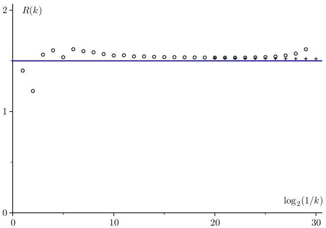
Figure 2. Approximation of $R(k)=\log(Z(k))/\log(k)$ based on truncating the sum in Eq. (13) to cube-free numbers $q$ that are multiples of the first $2^{13}$ square-free numbers (circles) and the first $2^{20}$ square-free numbers (crosses), respectively. The blue line corresponds to the ratio $3/2$.

The result of a numerical approximation to the sum in Eq. (13) is shown in Figure 2. Here, the sum over all cube-free numbers is rewritten as a sum over all square-free numbers and their cube-free multiples which share the same value of the function $f$ of Eq. (12). Truncated sums including up to $2^{20}$ square-free numbers are used, showing a behaviour that is close to the asymptotic form of $Z(k)$ from Eq. (14). Note that, due to the truncation of a sum of positive numbers, the numerical approximations for the ratio $R(k)=\log(Z(k))/\log(k)$, where $k\,\raisebox{2.0pt}{$\scriptscriptstyle\searrow$}\,0$, are always larger than the actual values, and apart from a couple of points at large values of $k$, all numerical estimates are above the asymptotic line. Also, since fewer terms contribute to the sums for smaller $k$, eventually the difference will become large for small $k$, as seen in Figure 2 for the data using fewer square-free numbers. A quantitive estimate of the error is difficult. For a more detailed analysis of this asymptotic behaviour, including power-free numbers for larger powers, we refer to [4].

4. Systems with absolutely continuous spectrum

The generic case for the emergence of absolutely continuous diffraction is the presence of some degree of randomness. This means that the most natural setting here is that of stochastic point processes, and quite a bit of work has recently been done; compare [26] and references therein.

Our goal in this section is modest in the sense that we only aim at collecting some one-dimensional results that are all well known, but rarely appear together. Moreover, we are not looking into the hyperuniform setting as in [26], but rather into systems that frequently appear in practice. For this reason, we keep also this section somewhat informal.

4.1. Poisson and Rudin–Shapiro

The homogeneous Poisson process with intensity (or point density) $1$ on the real line has diffraction measure $\widehat{\gamma}=\delta_{0}+\lambda_{\mathrm{L}}$, where $\lambda_{\mathrm{L}}$ denotes Lebesgue measure. This result applies to almost every realisation of this classic stochastic point process; see [11, Ex. 11.6]. This gives

(15) $$Z_{\text{P}}(k)\,=\,k$$

in this case, which can serve as a reference for the comparison with other stochastic processes.

The Bernoulli lattice gas on $\mathbb{Z}\hskip 0.5pt$ with occupation probability $p$ per site, see [11, Ex. 11.2], leads to $\widehat{\gamma}=p^{2}\delta_{\mathbb{Z}\hskip 0.5pt}+p(1-p)\lambda_{\mathrm{L}}$ for a.e. realisation, and hence to

$$Z(k)\,=\,p(1-p)k\hskip 0.5pt.$$

When using weights $\pm 1$ instead of $1$ and $0$, this changes to $\widehat{\gamma}=(2p-1)^{2}\delta_{\mathbb{Z}\hskip 0.5pt}+4p(1-p)\lambda_{\mathrm{L}}$ and thus to

$$Z(k)\,=\,4p(1-p)k$$

by [11, Prop. 11.1]. In particular, $p=\frac{1}{2}$ gives $Z(k)=k$ as for the Poisson process above. Similar results emerge for more general Bernoulli systems, where the slope of $Z$ is a measure of the point (or particle) density and of the variance of the underlying random variable; see [11, Rem. 11.1] for more.

The binary Rudin–Shapiro chain, when realised as a sequence with weights $\{\pm 1\}$, is a deterministic system with diffraction $\widehat{\gamma}=\lambda_{\mathrm{L}}$, and thus $Z(k)=k$ exactly; see [11, Thm. 10.2] and references given there. In particular, this system has linear complexity, as one can obtain it as a factor of a substitution rule on four letters [11, Sec. 4.7.1]. Note that these results apply to every element of the Rudin–Shapiro hull, which is minimal.

One can apply a simple Bernoullisation process [10] to the Rudin–Shapiro chain (or to any element of its hull). Given $p\in[0,1]$, one simply changes the sign at each site independently with probability $p$; see [11, Sec. 11.2.2] for the general setting and further details. By an application of [11, Prop. 11.2], the diffraction measure almost surely does not change, which means that we get

$$Z(k)\,=\,k\quad\text{for all }p\in[0,1]\hskip 0.5pt.$$

This is an interesting case of homometry, as one can continuously change the entropy of the system from $0$ (for $p=0$) to $\log(2)$ (for $p=\frac{1}{2}$, which really gives the fair coin tossing sequence with weights $\pm 1$). In particular, the (frequency weighted) patch complexity has no influence on $Z$ in this case. This highlights the limitation of this quantity (as well as that of the full diffraction measure) as a characterisation of order.

4.2. Random matrix ensembles

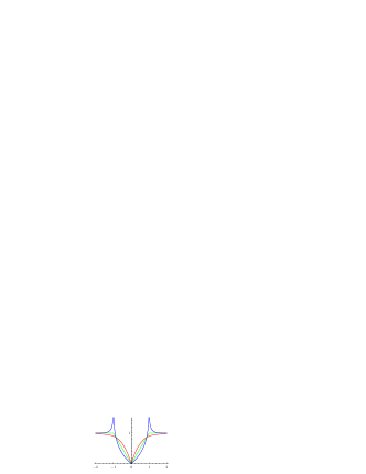
Figure 3. Absolutely continuous part of the diffraction measure for the classic random matrix ensembles with parameters $\beta=1$ (red), $\beta=2$ (green) and $\beta=4$ (blue).

The point processes (with point density $1$) derived from the classic random matrix ensembles with parameter $\beta$, compare [25] for background, can also be analysed for the scaling near $0$. Based on the calculations in [15], see also [11, Thm. 11.3], the scaling behaviour emerges from integrating the Radon–Nikodym densities, which are illustrated in Figure 3. The result reads

$$Z_{\beta}(k)\,=\,\begin{cases}k^{2}-\tfrac{2}{3}k^{3}+\mathcal{O}(k^{4}),&\text{for $\beta=1$},\\ \tfrac{1}{2}k^{2},&\text{for $\beta=2$},\\ \tfrac{1}{4}k^{2}+\tfrac{1}{12}k^{3}+\mathcal{O}(k^{4}),&\text{for $\beta=4$}.\end{cases}$$

The general behaviour is $Z_{\beta}(k)=\frac{1}{\beta}k^{2}+\mathcal{O}(k^{3})$, which significantly differs from the other cases discussed in this section. As $\beta\,\raisebox{2.0pt}{$\scriptscriptstyle\searrow$}\,0$, the leading term diverges, which indicates that one gets a different power law in this limit. Indeed, $\beta\,\raisebox{2.0pt}{$\scriptscriptstyle\searrow$}\,0$ gives the homogeneous Poisson process with unit density, with $Z_{\text{P}}(k)=k$ as in Eq. (15). In contrast, for $\beta\to\infty$, the leading term vanishes. This limit corresponds to the (deterministic) point process that realises the lattice $\mathbb{Z}\hskip 0.5pt$, where $Z(k)=0$ for all sufficiently small $k>0$.

4.3. Markov lattice gas

Let us consider a simple one-dimensional Markov lattice gas on $\mathbb{Z}\hskip 0.5pt$, as defined by

$$\raisebox{-18.0pt}{\includegraphics[width=130.08731pt]{markovgraph.eps}}\qquad\text{with Markov matrix}\quad M\,=\,\begin{pmatrix}p&1-p\\ 1-q&q\end{pmatrix},$$

where $p$ and $q$ are probabilities subject to the constraint $0<p+q<2$. The two states of the Markov chain correspond to empty (weight $0$) and occupied (weight $1$) sites. Interpreted as a lattice gas, we almost surely get a particle system of density $\varrho=\frac{1-p}{2-p-q}$.

Employing the results from [11, Ex. 11.11], we know that the absolutely continuous part of the diffraction measure, $\widehat{\gamma}_{\text{ac}}$, is almost surely represented by the Radon–Nikodym density

$$g(k)\,=\,\frac{(1-p)(1-q)(1+r)}{(1-r)(1-2\hskip 0.5ptr\cos(2\pi k)+r^{2})}\,,$$

where $r=p+q-1$, which satisfies $|r|<1$ by our assumption. A straightforward calculation gives

(16) $$Z(k)\,=\,g(0)\Bigl{(}k-\frac{\raisebox{-2.0pt}{$4\hskip 0.5pt\pi^{2}$}}{\raisebox{0.5pt}{$3$}}\hskip 0.5pt\frac{\raisebox{-2.0pt}{$r$}}{\raisebox{0.5pt}{$(1-r)^{2}$}}\,k^{3}+\mathcal{O}(k^{5})\Bigr{)}$$

with $g(0)=\frac{(1-p)(1-q)(1+r)}{(1-r)^{3}}\geqslant 0$. When $r=0$, Eq. (16) simplifies to

$$Z(k)\,=\,(1-p)(1-q)\hskip 0.5ptk\hskip 0.5pt.$$

Note that $r<0$ and $r>0$ correspond to effectively repulsive and attractive systems, respectively; see Figure 4 for an illustration of $g$ for these two situations.

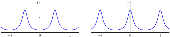
Figure 4. Absolutely continuous part of the Markov chain diffraction. The left panel shows the case $p=q=\frac{1}{4}$, which is effectively repulsive, with parameter $r=-\frac{1}{2}$. The right panel shows the corresponding effectively attractive case for $p=q=\frac{3}{4}$, with $r=\frac{1}{2}$.

4.4. Binary random tilings on the line

To keep things simple, let us consider a random tiling of $\mathbb{R}$ that is built from just two intervals (of lengths $u$ and $v$, say) with corresponding probabilities $p$ and $q=1-p$. We place a scatterer of unit strength at the left endpoint of each interval. Then, almost surely, the diffraction comprises a pure point and an absolutely continuous component, see [11, Thm. 11.6], where only the latter contributes to the scaling of $Z(k)$ near $0$. By a straightforward integration, as $k\,\raisebox{2.0pt}{$\scriptscriptstyle\searrow$}\,0$, one obtains

$$Z(k)\,=\,\frac{p\hskip 0.5ptq(u-v)^{2}}{(pu+qv)^{3}}\left(k+\frac{\pi^{2}}{9}\hskip 0.5pt\frac{u^{2}v^{2}-2u\hskip 0.5ptv(pu^{2}+qv^{2})}{p\hskip 0.5ptq(u-v)^{2}-(pu^{2}+qv^{2})}\,k^{3}+\mathcal{O}(k^{5})\right),$$

which is non-trivial only for $u\neq v$. For $u=v$, the resulting point set is always periodic, and $Z(k)=0$ for all sufficiently small $k>0$.

Note that, as in all other examples of this section, $Z(k)$ is a continuous function, and one can often determine both the scaling exponent and the corresponding coefficient explicitly. While the continuity persists for singular continuous $\widehat{\gamma}$, determining the constant will generally be more complicated.

5. Singular continuous measures

Let us finally consider the case of structures with singular continuous diffraction. While this seems a rare phenomenon in practice, such systems are actually generic in some sense (in particular among substitution systems), and thus deserve more attention.

5.1. The Thue –Morse measure

The singular continuous Thue –Morse (TM) measure $\mu_{\mathrm{TM}}$ is defined as an infinite Riesz product [37, 11],

$$\mu_{\mathrm{TM}}\,=\prod_{\ell=0}^{\infty}\bigl{(}1-\cos(2^{\ell+1}\pi x)\bigr{)},$$

which is to be understood as a limit in the vague topology; we refer to [11, Ch. 10.1] and references therein for background and notation. Note that $\mu_{\mathrm{TM}}$ is a probability measure on $\mathbb{T}=\mathbb{R}/\mathbb{Z}\hskip 0.5pt$, which is the viewpoint from dynamical systems. It is connected to the diffraction measure $\widehat{\gamma}_{\mathrm{TM}}$ on $\mathbb{R}$ via

$$\widehat{\gamma}_{\mathrm{TM}}\,=\,\mu_{\mathrm{TM}}*\delta_{\mathbb{Z}\hskip 0.5pt}\hskip 0.5pt,$$

under the obvious identification of $\mathbb{T}$ with $[0,1)$ and addition modulo $1$. For the investigation of $Z(k)$ for small $k$, we can thus simply work with $\mu_{\mathrm{TM}}$.

More concretely, for $n\in\mathbb{N}_{0}$, we consider the functions

$$f_{n}(x)\,=\prod_{\ell=0}^{n-1}\bigl{(}1-\cos(2^{\ell+1}\pi x)\bigr{)},$$

which are probability densities on the unit interval, where $f_{0}(x)=1$ as usual. They satisfy

(17) $$f_{n+m}(x)\,=\,f_{n}(x)\,f_{m}(2^{n}x)$$

for all $n,m\in\mathbb{N}_{0}$. Since $f_{n}(x)=f_{n}(1-x)$, one also has

(18) $$\int_{0}^{1}\!x\,f_{n}(x)\,\mathrm{d}x\,=\,\frac{\raisebox{-2.0pt}{$1$}}{\raisebox{0.5pt}{$2$}}$$

for all $n\in\mathbb{N}_{0}$. The corresponding distribution functions

$$F_{n}(k)\,=\int_{0}^{k}\!\,\mathrm{d}F_{n}(x)\,=\int_{0}^{k}\!f_{n}(x)\,\mathrm{d}x$$

converge uniformly to the distribution function $F(x)\mathrel{\mathop{:}}=\mu_{\mathrm{TM}}\bigl{(}[0,k]\bigr{)}$, which is a continuous function on $[0,1]$ with $F(0)=0$ and $F(1)=1$. In fact, $F$ is strictly increasing and satisfies the symmetry relation $F(1-k)=1-F(k)$. Moreover, $F$ possesses the uniformly converging Fourier series representation [11, Eq. 10.9]

$$F(k)\,=\,k\,+\sum_{m=1}^{\infty}\frac{\eta(m)}{m\pi}\hskip 0.5pt\sin(2\pi mk)\hskip 0.5pt,$$

where the $\eta(m)$ are the Fourier coefficients of $\mu_{\mathrm{TM}}$. Note that the $\eta(m)$ are also the pair correlation coefficients of the Thue –Morse sequence when realised with weights $\pm 1$. They are recursively specified by $\eta(0)=1$ together with

$$\eta(2m)\,=\,\eta(m)\quad\text{and}\quad\eta(2m+1)\,=\,-\frac{\raisebox{-2.0pt}{$1$}}{\raisebox{0.5pt}{$2$}}\bigl{(}\eta(m)+\eta(m+1)\bigr{)}$$

for $m\in\mathbb{N}_{0}$. In particular, this entails $\eta(1)=-\frac{1}{3}$, while all other values then follow recursively.

To study $Z(k)=F(k)$ for small $k$, compare [9], it suffices to analyse the behaviour of $F$ along sequences $(2^{-n})_{n\in\mathbb{N}}$ because $F$ is strictly increasing and continuous. Let $N\geqslant n$ and observe

(19) $$\begin{split}F_{N}(2^{-n})\,&=\int_{0}^{2^{-n}}\!\!\!f_{N}(x)\,\mathrm{d}x\,\stackrel{{\scriptstyle\eqref{eq:f-split}}}{{=}}\int_{0}^{2^{-n}}\!\!\!f_{n}(x)\,f_{N-n}(2^{n}x)\,\mathrm{d}x\\[5.69054pt] &\leqslant\sup\big{\{}f_{n}(x):x\in[0,2^{-n}]\big{\}}\;2^{-n}\!\int_{0}^{1}\!f_{N-n}(y)\,\mathrm{d}y\,=\,2^{-n}f_{n}(2^{-n})\hskip 0.5pt,\end{split}$$

where the last step uses that $f_{n}$ is increasing on $[0,2^{-n}]$. In the other direction, one gets

(20) $$\begin{split}F_{N}(2^{-n})\,&=\,2^{-n}\!\int_{0}^{1}f_{n}(2^{-n}y)\,f_{N-n}(y)\,\mathrm{d}y\\[5.69054pt] &\geqslant\,2^{-n}f_{n}\biggl{(}2^{-n}\!\int_{0}^{1}\!y\,f_{N-n}(y)\,\mathrm{d}y\biggr{)}\,\stackrel{{\scriptstyle\eqref{eq:expect}}}{{=}}\,2^{-n}f_{n}(2^{-n-1})\hskip 0.5pt,\end{split}$$

where the estimate follows from Jensen’s inequality, as $f_{n}(2^{-n}x)$ is convex on $[0,1]$.

Remark 5.1.

One can improve the lower bound by splitting the integral as

$$F_{N}(2^{-n})\,=\,2^{-n}\!\int_{0}^{\frac{1}{2}}f_{n-1}(2^{-n+1}y)\,2\hskip 0.5ptf_{N-n+1}(y)\,\mathrm{d}y\,\geqslant\,2^{-n}f_{n-1}(2^{-n+1}\beta_{N-n+1})$$

with $\beta_{N-n+1}=2\int_{0}^{1/2}y\hskip 0.5ptf_{N-n+1}(y)\,\mathrm{d}y$. This trick uses the fact that $2f_{n}(x)$ is a probability density on $\bigl{[}0,\frac{1}{2}\bigr{]}$, as a consequence of the reflection symmetry. Taking the limit as $N\to\infty$, one obtains the estimate $F(2^{-n})\geqslant 2^{-n}f_{n-1}(2^{-n+1}\beta)$ with

$$\beta\,=\,\frac{\raisebox{-2.0pt}{$1$}}{\raisebox{0.5pt}{$4$}}-\frac{\raisebox{-2.0pt}{$2$}}{\raisebox{0.5pt}{$\pi^{2}$}}\sum_{m\geqslant 0}\frac{\eta(2m+1)}{(2m+1)^{2}}\,\approx\,0.30994\hskip 0.5pt,$$

as can be calculated with the Fourier series representation of $F$. $\Diamond$

So far, by taking $N\to\infty$, we have the bounds

(21) $$2^{-n}f_{n}(2^{-n-1})\,\leqslant\,F(2^{-n})\,\leqslant\,2^{-n}f_{n}(2^{-n})\hskip 0.5pt,$$

where the lower one can be improved as explained in Remark 5.1. For small $x$, a series expansion analysis of $f_{n}$ gives

$$f_{n}(x)\,=\,2^{n^{2}}(\pi x)^{2n}\Bigl{(}1-\frac{\raisebox{-2.0pt}{$4^{n}-1$}}{\raisebox{0.5pt}{$9$}}(\pi x)^{2}+\frac{\raisebox{-2.0pt}{$11\cdot 16^{n}-25\cdot 4^{n}+14$}}{\raisebox{0.5pt}{$2015$}}(\pi x)^{4}+\mathcal{O}\bigl{(}x^{6}\bigr{)}\Bigr{)}.$$

With a bit more work, for $x=2^{-n}$, one can now establish the asymptotic behaviour

(22) $$2^{-n}f_{n}(2^{-n})\,\sim\,c\,2^{-n^{2}}\Bigl{(}\frac{\raisebox{-2.0pt}{$\pi^{2}$}}{\raisebox{0.5pt}{$2$}}\Bigr{)}^{n}\qquad\text{as $n\to\infty$},$$

with $c\approx 0.306{\hskip 0.5pt}663$. The constant was calculated numerically from the quickly converging sequence of quotients. Note that the right-hand side of Eq. (22) decays faster than any power of $2^{-n}$, which means that we will not get a power law for the scaling of $F(k)$ as $k\,\raisebox{2.0pt}{$\scriptscriptstyle\searrow$}\,0$. Similarly, one obtains the asymptotic behaviour

(23) $$2^{-n}f_{n}(2^{-n-1})\,\sim\,\frac{\raisebox{-2.0pt}{$\pi^{2}c$}}{\raisebox{0.5pt}{$4$}}\,2^{-n^{2}}\Bigl{(}\frac{\raisebox{-2.0pt}{$\pi^{2}$}}{\raisebox{0.5pt}{$8$}}\Bigr{)}^{n}\qquad\text{as $n\to\infty$},$$

with the same constant $c$, hence $\frac{\pi^{2}c}{4}\approx 0.756{\hskip 0.5pt}660$.

It remains to express the result in terms of $k=2^{-n}$, via $\log(k)=-n\log(2)$. From Eqs. (22) and (23), in conjunction with the continuity and monotonicity of $F$, one obtains the following result.

Theorem 5.2.

The distribution function $F$ of the Thue –Morse measure satisfies the asymptotic bounds

$$c_{1}k^{2+\alpha}\exp\Bigl{(}-\frac{\raisebox{-2.0pt}{$\log(k)^{2}$}}{\raisebox{0.5pt}{$\log(2)$}}\Bigr{)}\,\leqslant\,F(k)\,\leqslant\,c_{2}\hskip 0.5ptk^{\alpha}\hskip 0.5pt\exp\Bigl{(}-\frac{\raisebox{-2.0pt}{$\log(k)^{2}$}}{\raisebox{0.5pt}{$\log(2)$}}\Bigr{)}$$

for small $k>0$, with exponent

$$\alpha\,=\,-\frac{\log\bigl{(}\frac{\pi^{2}}{2}\bigr{)}}{\log(2)}\,\approx\,-2.302{\hskip 0.5pt}992$$

and suitable constants $c_{1}$, $c_{2}$.∎

A similar estimate, with the same leading term, was previously given in [27]. Some numerical experiments indicate that the upper bound is better then the lower one (which can be improved by Remark 5.1), and that the true behaviour is closer to a prefactor of the form $k^{\alpha+s}$ with $s$ near $\frac{1}{2}$, which deserves further analysis.

5.2. Generalised Thue –Morse (gTM) sequences

Let us finally consider the family of binary, primitive, constant-length substitutions $\varrho_{p,q}\!:a\mapsto a^{p}b^{q},b\mapsto b^{\hskip 0.5ptp}a^{q}$ with $p,q\in\mathbb{N}$; see [7] for a general exposition and [11, Ex. 10.1] for a short summary. The case $p=q=1$ is the classic Thue –Morse substitution considered above. In what follows, we suppress the explicit dependence on $p$ and $q$ for ease of notation.

Figure 5. Distribution functions $F(k)$ of the gTM measures for $(p,1)$ with $p\in\{1,3,5\}$ and the behaviour at small $k$ for $p\in\{1,2,3,4,5\}$ (inset). Dashed lines indicate the scaling behaviour from Eq. (26) for $p\in\{2,3,4,5\}$.

Here, the spectral measure is given by the Riesz product $\mu=\prod_{m\geqslant 0}\vartheta\bigl{(}(p+q)^{m}x\bigr{)}$ with the non-negative trigonometric polynomial

(24) $$\vartheta(x)\,=\,1+\frac{\raisebox{-2.0pt}{$2$}}{\raisebox{0.5pt}{$p+q$}}\sum_{r=1}^{p+q-1}\alpha(p,q,r)\,\cos(2\pi rx)\hskip 0.5pt,$$

where $\alpha(p,q,r)=p+q-r-2\hskip 0.5pt\min(p,q,r,p+q-r)$. For $x\to 0$, $\vartheta$ behaves as

(25) $$\vartheta(x)\,=\,\frac{(p-q)^{2}}{p+q}+\frac{12\hskip 0.5ptp^{2}q^{2}+(p-q)^{2}-(p-q)^{4}}{3(p+q)}\hskip 0.5pt(\pi x)^{2}+\mathcal{O}(x^{4})\hskip 0.5pt.$$

Whenever $p=q$, we have $\vartheta(0)=0$, and we are in a situation similar to that of the classic Thue –Morse sequence. Otherwise, $\vartheta(0)>0$, where this value can be less than $1$, precisely $1$ or larger than $1$. Nevertheless, all these cases can be treated by the same approach. Defining $f_{n}(x)=\prod_{m=0}^{n-1}\vartheta\bigl{(}(p+q)^{m}x\bigr{)}$, one has

$$f_{n+m}(x)\,=\,f_{n}(x)\,f_{m}\bigl{(}(p+q)^{n}x\bigr{)}$$

for arbitrary $m,n\in\mathbb{N}_{0}$. In particular, this gives

$$f_{n+m}\Bigl{(}\frac{\raisebox{-2.0pt}{$x$}}{\raisebox{0.5pt}{$(p+q)^{n}$}}\Bigr{)}\,=\,\vartheta\Bigl{(}\frac{\raisebox{-2.0pt}{$x$}}{\raisebox{0.5pt}{$(p+q)^{n}$}}\Bigr{)}\,f_{n+m-1}\Bigl{(}\frac{\raisebox{-2.0pt}{$x$}}{\raisebox{0.5pt}{$(p+q)^{n-1}$}}\Bigr{)}.$$

Since $\lim_{n\to\infty}\vartheta\bigl{(}(p+q)^{-n}x\bigr{)}=\vartheta(0)$, we see that, for any fixed $m$, the limit

$$\lim_{n\to\infty}\vartheta(0)^{-n}f_{n+m}\bigl{(}(p+q)^{-n}x\bigr{)}$$

exists. By standard arguments, this implies the asymptotic behaviour

$$F\bigl{(}(p+q)^{-n}\bigr{)}\,\sim\,\biggl{(}\frac{p+q}{\vartheta(0)}\biggr{)}^{\!-n}\qquad\text{as $n\to\infty$.}$$

Since $F$ is continuous and increasing, using $\vartheta(0)=(p-q)^{2}/(p+q)$, one finds the scaling behaviour

(26) $$Z(k)\,=\,F(k)\,\sim\,k^{2-2\frac{\log|p-q|}{\log(p+q)}}\qquad\text{as $k\,\raisebox{2.0pt}{$\scriptscriptstyle\searrow$}\,0\hskip 0.5pt$,}$$

which is in agreement with the scaling argument from [27] and Conjecture 3 in [35]. For $p\neq q$, the exponent can be $2$, $1$ or take positive values below $1$ that can become arbitrarily small. The corresponding behaviour for small $k$ matches well with the examples from [7] and [11, Fig. 10.2], as illustrated in Figure 5 for some characteristic choices of the parameters.

6. Concluding remarks

The situation for one-dimensional systems is in reasonably good shape, though a better understanding is still desirable. This is particularly so for multi-type systems, where the existing approach gives bounds but not necessarily the exact asymptotic behaviour.

Less clear is the appropriate approach to analyse tilings and point processes in higher dimension, where one could single out special directions, but also consider the total diffraction into regions near the origin. This should be possible within the realm of both inflation tilings and projection point sets.

References

- [1] Alcaraz F C, Baake M, Grimm U and Rittenberg V, Operator content of the XXZ chain, J. Phys. A: Math. Gen. 21 (1988) L117–L120.
- [2] Alcaraz F C and Rittenberg V, Shared information in stationary states at criticality, J. Stat. Mech. (2010) P03024:1–28; arXiv:0912.2963.
- [3] Aubry S, Godrèche C and Luck J M, Scaling properties of a structure intermediate between quasiperiodic and random, J. Stat. Phys. 51 (1988) 1033–1074.
- [4] Baake M and Coons M, Scaling of the diffraction measure of -free integers near the origin, preprint (2019); arXiv:1904.00279.
- [5] Baake M, Frank N P, Grimm U and Robinson E A, Geometric properties of a binary non-Pisot inflation and absence of absolutely continuous diffraction, Studia Math. 247 (2019) 109–154; arXiv:1706.03976.
- [6] Baake M and Gähler F, Pair correlations of aperiodic inflation rules via renormalisation: Some interesting examples, Topol. & Appl. 205 (2016) 4–27; arXiv:1511.00885.
- [7] Baake M, Gähler F and Grimm U, Spectral and topological properties of a family of generalised Thue –Morse sequences, J. Math. Phys. 53 (2012) 032701:1–24; arXiv:1201.1423.
- [8] Baake M, Gähler F and Mañibo N, Renormalisation of pair correlation measures for primitive inflation rules and absence of absolutely continuous diffraction, Commun. Math. Phys., in press; arXiv:1805.09650.
- [9] Baake M, Gohlke P, Kesseböhmer M and Schindler T, Scaling properties of the Thue –Morse measure, Discr. Cont. Dynam. Syst. A 39 (2019) 4157–4185; arXiv:1810:06949.
- [10] Baake M and Grimm U, Kinematic diffraction is insufficient to distinguish order from disorder, Phys. Rev. B 79 (2009) 020203(R):1–4 and Phys. Rev. B 80 (2009) 029903(E); arXiv:0810.5750.
- [11] Baake M and Grimm U, Aperiodic Order. Vol. : A Mathematical Invitation, Cambridge University Press, Cambridge (2013).
- [12] Baake M and Grimm U (eds.), Aperiodic Order. Vol. : Crystallography and Almost Periodicity, Cambridge University Press, Cambridge (2017).
- [13] Baake M, Grimm U and Mañibo N, Spectral analysis of a family of binary inflation rules, Lett. Math. Phys. 108 (2018) 1783–1805; arXiv:1709.09083.
- [14] Baake M, Huck C and Strungaru N, On weak model sets of extremal density, Indag. Math. 28 (2017) 3–31; arXiv:1512.07129.
- [15] Baake M and Kösters H, Random point sets and their diffraction, Philos. Mag. 91 (2011) 2671–2679; arXiv:1007.3084.
- [16] Baake M and Lenz D, Spectral notions of aperiodic order, Discr. Cont. Dynam. Syst. S 10 (2017) 161–190; arXiv:1601.06629.
- [17] Baake M, Moody R V and Pleasants P A B, Diffraction of visible lattice points and th power free integers, Discr. Math. 221 (2000) 3–42; arXiv:math.MG/9906132.
- [18] Baake M, Moody R V and Schlottmann M, Limit-(quasi)periodic point sets as quasicrystals with -adic internal spaces, J. Phys. A: Math. Gen. 31 (1998) 5755–5765; arXiv:math-ph/9901008.
- [19] Baake M and Sing B, Kolakoski- is a (deformed) model set, Can. Math. Bull. 47 (2004) 168–190; arXiv:math.MG/0206098.
- [20] Barreira L and Pesin Y, Nonuniform Hyperbolicity, Cambridge University Press, Cambridge (2007).
- [21] Bufetov A and Solomyak B, On the modulus of continuity for spectral measures in substitution dynamics, Adv. Math. 260 (2014) 84–129; arXiv:1305.7373.
- [22] Bufetov A and Solomyak B, A spectral cocycle for substitution systems and translation flows, preprint arXiv:1802.04783.
- [23] de Gier J, Nichols A, Pyatov P and Rittenberg V, Magic in the spectra of the XXZ quantum chain with boundaries at and , Nucl. Phys. B 729 (2005) 387–418; arXiv:hep-th/0505062.
- [24] de Gier J, Nienhuis B, Pearce P A and Rittenberg V, Stochastic processes and conformal invariance, Phys. Rev. E 67 (2003) 016101:1–4; arXiv:cond-mat/0205467.
- [25] Forrester P, Log-Gases and Random Matrices, Princeton University Press, Princeton (2010).
- [26] Ghosh S and Lebowitz J L, Generalized stealthy hyperuniform processes: Maximal rigidity and the bounded holes conjecture, Commun. Math. Phys. 363 (2018) 97–110; arXiv:1707.04328.
- [27] Godrèche C and Luck J M, Multifractal analysis in reciprocal space and the nature of the Fourier transform of self-similar structures, J. Phys. A: Math. Gen. 23 (1990) 3769–3797.
- [28] Hof A, On diffraction by aperiodic structures, Commun. Math. Phys. 169 (1995) 25–43.
- [29] Keller G and Richard C, Periods and factors of weak model sets, Israel J. Math. 229 (2019) 85–132; arXiv:1702.02383.
- [30] Lenz D, Continuity of eigenfunctions of uniquely ergodic dynamical systems and intensity of Bragg peaks, Commun. Math. Phys. 287 (2009) 225–258; arXiv:math-ph/0608026.
- [31] Luck J M, A classification of critical phenomena on quasi-crystals and other aperiodic structures, Europhys. Lett. 24 (1993) 359–364.
- [32] Mañibo N, Spectral analysis of primitive inflation rules, Oberwolfach Rep. 14 (2017) 2830–2832.
- [33] Moody R V and Strungaru N, Almost periodic measures and their Fourier transforms, in [12], pp. 173–270.
- [34] Oğuz E C, Socolar J E S, Steinhardt P J and Torquato S, Hyperuniformity of quasicrystals, Phys. Rev. B 95 (2017) 054119:1–10; arXiv:1612:01975.
- [35] Oğuz E C, Socolar J E S, Steinhardt P J and Torquato S, Hyperuniformity and anti-hyperuniformity in one-dimensional substitution tilings, Acta Cryst. A 75 (2019) 3–13; arXiv:1806.10641.
- [36] Pleasants P A B and Huck C, Entropy and diffraction of the -free points in -dimensional lattices, Discr. Comput. Geom. 50 (2013) 39–68; arXiv:1112.1629.
- [37] Queffélec M, Substitution Dynamical Systems — Spectral Analysis, 2nd ed., LNM 1294, Springer, Berlin (2010).
- [38] Solomyak B, Dynamics of self-similar tilings, Ergod. Th. & Dynam. Syst. 17 (1997) 695–738 and Ergod. Th. & Dynam. Syst. 19 (1999) 1685 (erratum).
- [39] Torquato S and Stillinger F H, Local density fluctuations, hyperuniformity, and order metrics, Phys. Rev. E 68 (2003) 041113:1–25 and Phys. Rev. E 68 (2003) 069901 (erratum); arXiv:cond-mat/0311532.
- [40] Viana M, Lectures on Lyapunov Exponents, Cambridge University Press, Cambridge (2013).