Formal Verification of Input-Output Mappings of Tree Ensembles

Abstract

Recent advances in machine learning and artificial intelligence are now being considered in safety-critical autonomous systems where software defects may cause severe harm to humans and the environment. Design organizations in these domains are currently unable to provide convincing arguments that their systems are safe to operate when machine learning algorithms are used to implement their software.

In this paper, we present an efficient method to extract equivalence classes from decision trees and tree ensembles, and to formally verify that their input-output mappings comply with requirements. The idea is that, given that safety requirements can be traced to desirable properties on system input-output patterns, we can use positive verification outcomes in safety arguments. This paper presents the implementation of the method in the tool VoTE (Verifier of Tree Ensembles), and evaluates its scalability on two case studies presented in current literature. We demonstrate that our method is practical for tree ensembles trained on low-dimensional data with up to 25 decision trees and tree depths of up to 20. Our work also studies the limitations of the method with high-dimensional data and preliminarily investigates the trade-off between large number of trees and time taken for verification.

1 Introduction

In recent years, artificial intelligence utilizing machine learning algorithms has begun to outperform humans at several tasks, e.g., playing board games [29] and diagnosing skin cancer [10]. These advances are now being considered in safety-critical autonomous systems where software defects may cause severe harm to humans and the environment, e.g, airborne collision avoidance systems [16].

Several researchers have raised concerns [5, 19, 26] regarding the lack of verification methods for these kinds of systems in which machine learning algorithms are used to train software deployed in the system. Within the avionics sector, guidelines [7] describe how design organizations may apply formal methods to the verification of safety-critical software. Applying these methods to complex and safety-critical software is a non-trivial task due to practical limitations in computing power and challenges in qualifying complex verification tools. These challenges are often caused by a high expressiveness provided by the language in which the software is implemented in. Most research that apply formal methods to the verification of machine learning is so far focused on the verification of neural networks, but there are other models that may be more appropriate when verifiability is important, e.g., decision trees [3], random forests [4] and gradient boosting machines [11]. Where neural networks are subject to verification of correctness, they are usually adopted in non-safety-critical cases, e.g., fairness with respect to individual discrimination, where probabilistic guarantees are plausible [2]. Since our aim is to support safety arguments for digital artefacts that may be deployed in hazardous situations, we need to rely on guarantees of absence of misclassifications, or at least recognize when such guarantees cannot be provided. The tree-based models provide such an opportunity since their structural simplicity makes them easy to analyze systematically, but large (yet simple) models may still prove hard to verify due to combinatorial explosion.

This paper is an improved and substantially extended version of our previous work [31]. In that work, we developed a method to partition the input domain of decision trees into disjoint sets, and to explore all path combinations in random forests in such a way that counteracts combinatorial path explosions. In this paper, we generalize the method to also apply to gradient boosting machines and implement it in a tool named VoTE. The paper also evaluates the tool with respect to performance. The VoTE source code (which includes automation of the case studies) is published as free software. Compared to previous works, the contributions of this paper are as follows.

• A generalization to include more tree ensembles, e.g., gradient boosting machines, with an updated tool support (VoTE).

• A Soundness proof of the associated approximation technique used for this purpose.

• An improved node selection strategy that yields speed improvements in the range of 4 %–91 % for trees with a depth of $10$ or more in the two demonstrated case studies.

The rest of this paper is structured as follows. Section 2 presents preliminaries on decision trees, tree ensembles, and a couple of interesting properties subject to verification. Section 3 discusses related works on formal verification and machine learning, and Section 4 presents our method with our supporting tool VoTE. Section 5 presents applications of our method on two case studies; a collision detection problem, and a digit recognition problem. Finally, Section 6 concludes the paper and summarizes the lessons we learned.

2 Preliminaries

In this section, we present preliminaries on different machine learning models and their properties that we consider for verification in this paper.

2.1 Decision Trees

In machine learning, decision trees are used as predictive models to capture statistical properties of a system of interest.

Definition 1 (Decision Tree)

A decision tree implements a prediction function $t:X^{n}\rightarrow\mathbb{R}^{m}$ that maps disjoint sets of points $X_{i}\subset X^{n}$ to a single output point $\bar{y}_{i}\in\mathbb{R}^{m}$, i.e.,

$$t(\bar{x})=\begin{cases}(y_{1,1},\ldots,y_{1,m})&\bar{x}\in X_{1}\\ \hfill\vdots\\ (y_{k,1},\ldots,y_{k,m})&\bar{x}\in X_{k},\\ \end{cases}$$

where $k$ is the number of disjoint sets and $X^{n}=\bigcup\limits_{i=1}^{k}X_{i}$.

For perfectly balanced binary decision trees, $k=2^{d}$, where $d$ is the tree depth. Each internal node is associated with a decision function that separates points in the input space from each other, and the leaves define output values. The n-dimensional input domain $X^{n}$ includes elements $\bar{x}$ as tuples in which each element ${x}_{i}$ captures some feature of the system of interest as an input variable. The tree structure is evaluated in a top-down manner, where decision functions determine which path to take towards the leaves. When a leaf is hit, the output $\bar{y}\in\mathbb{R}^{m}$ associated with the leaf is emitted. Figure 1 depicts a decision tree with one decision function ($x\leq 0$) and two outputs (1 and 2).

Figure 1: A decision tree with two possible outputs, depending on the value of single input variable $x$.

In general, decision functions are defined by non-linear combinations of several input variables at each internal node. In this paper, we only consider binary trees with linear decision functions with one input variable, which Irsoy et al. call univariate hard decision trees [14]. As illustrated by Figure 2, a univariate hard decision tree forms hyperrectangles (boxes) that split the input space along axes in the coordinate system.

Figure 2: The input space of a univariate hard decision tree, which splits the input space along axes in the coordinate system, thus forming boxes.

Although researchers have demonstrated that non-linear [14] and multivariate decision trees [32] can be useful, state-of-the-art implementations of tree ensembles normally use hard univariate decision trees, e.g., scikit-learn [23] and CatBoost [24].

2.2 Random Forests

Decision trees are known to suffer from a phenomenon called overfitting. Models suffering from this phenomenon can be fitted so tightly to their training data that their performance on unseen data is reduced the more you train them. To counteract these effects in decision trees, Breiman [4] proposes random forests.

Definition 2 (Random Forest)

A random forest implements a prediction function $f_{\mathit{rf}}:X^{n}\rightarrow\mathbb{R}^{m}$ as the arithmetic mean of the predictions from $B$ decision trees, i.e.,

$$f_{\mathit{rf}}(\bar{x})=\frac{1}{B}\sum\limits_{b=1}^{B}t_{b}(\bar{x}),$$

where $t_{b}$ is the $b$-th tree.

To reduce correlation between trees, each tree is trained on a random subset of the training data, using potentially overlapping random subsets of the input variables.

2.3 Gradient Boosting Machines

Similarly, Freidman [11] introduces a machine learning model called gradient boosting machine that uses several decision trees to implement a prediction function. Unlike random forests, these trees are trained in a sequential manner. Each consecutive tree tries to compensate for errors made by previous trees by estimating the gradient of errors (using gradient decent, hence the name).

Definition 3 (Gradient Boosting Machine)

A gradient boosting machine implements a prediction function $f_{\mathit{gb}}:X^{n}\rightarrow\mathbb{R}^{m}$ as the sum of predictions from $B$ decision trees, i.e.,

$$f_{\mathit{gb}}(\bar{x})=\sum\limits_{b=1}^{B}t_{b}(\bar{x}),$$

where $t_{b}$ is the $b$-th tree.

Typically, trees in a gradient boosting machine are significantly shallower than trees in a random forest, often with a tree depth in the range 2–10. Gradient boosting machines instead capture complexity by growing more trees.

2.4 Tree Ensemble

The learning algorithms used in random forests and gradient boosting machines are conceptually different from each other. However, once training is completed, the prediction functions which are the subjects to verification in this paper are similar. In a verification context, random forests and gradient boosting machines can therefore be generalized as instances of a tree ensemble.

Definition 4 (Tree Ensemble)

A tree ensemble implements a prediction function $f:X^{n}\rightarrow\mathbb{R}^{m}$ as the sum of predictions from $B$ decision trees, post-processed by a function $p:\mathbb{R}^{m}\rightarrow\mathbb{R}^{m}$, i.e.,

$$f(\bar{x})=p\Big{(}\sum\limits_{b=1}^{B}t_{b}(\bar{x})\Big{)},$$

where $t_{b}$ is the $b$-th tree.

In a verification context, the only conceptual difference between a random forest and gradient boosting machine is the post-processing function $p$, i.e., a constant division $p(\bar{y})=\frac{\bar{y}}{B}$ in the case of random forests, and the identity function $p(\bar{y})=\bar{y}$ in the case of gradient boosting machines.

2.5 Classifiers

Decision trees and tree ensembles may also be used as classifiers. A classifier is a function that categorizes samples from an input domain into one or more classes. In this paper, we only consider functions that map each point from an input domain to exactly one class.

Definition 5 (Classifier)

Let $f(\bar{x})=(y_{1},\ldots,y_{m})$ be a model trained to predict the probability $y_{i}$ associated with a class $i$ within disjoint regions in the input domain, where $m$ is the number of classes. Then we would expect that $\forall i\in\{1,\ldots,m\},0\leq y_{i}\leq 1$, and $\sum\limits_{i=1}^{m}y_{i}=1$. A classifier $f_{c}(\bar{x})$ may then be defined as

$$f_{c}(\bar{x})=\operatorname*{argmax}_{i}y_{i}.$$

A random forest typically infers probabilities by capturing the number of times a particular class has been observed within some hyperrectangle in the input domain of a tree during training. Training a gradient boosting machine to predict class membership probabilities is somewhat different, depending on the characteristics of the used learning algorithm, and often involves additional post-processing of the sum of all trees. For example, when training multiclass classifiers in CatBoost [24], individual trees emit values from a logarithmic domain that are summed up, and finally transformed and normalized into probabilities using the $\operatorname*{softmax}$ function, i.e.,

$$p(\bar{y})=\operatorname*{softmax}(y_{1},\ldots,y_{m})=\frac{(e^{y_{1}},\ldots,e^{y_{m}})}{\sum\limits_{i=1}^{m}y_{i}}$$

2.6 Safety Properties

In this paper, we consider two properties commonly used in related works; robustness against noise and plausibility of range. Note that compliance with these two properties alone is generally not sufficient to ensure safety. System safety engineers typically define requirements on software functions that are richer than these two properties alone.

Property 1 (Robustness against Noise)

Let $f:X^{n}\rightarrow\mathbb{R}^{m}$ be the function subject to verification, $\epsilon\in\mathbb{R}_{\geq 0}$ a robustness margin, and $\Delta=\{\delta\in\mathbb{R}:-\epsilon<\delta<\epsilon\}$ noise. We denote by $\bar{\delta}$ an $n$-tuple of elements drawn from $\Delta$. The function is robust against noise iff

$$\forall\bar{x}\in X^{n},\;\;\forall\bar{\delta}\in\Delta^{n},f(\bar{x})=f(\bar{x}+\bar{\delta}).$$

Pulina and Tacchella [25] define a stability property that is similar to our notion of robustness here but use scalar noise.

Property 2 (Plausibility of Range)

Let $f:X^{n}\rightarrow\mathbb{R}^{m}$ be the function subject to verification. The function has a desired plausibility of range when its output values are within a stated boundary, i.e.,

$$\forall\bar{x}\in X^{n},\forall i\in\{1,\ldots,m\},f(\bar{x})=(y_{1},\ldots,y_{m}),\;\;\alpha_{i}\leq y_{i}\leq\beta_{i}.$$

for some $\alpha_{i},\beta_{i}\in\mathbb{R}$.

In classification problems, the output tuple $(y_{1},\ldots,y_{m})$ contains probabilities, and thus $\alpha_{i}=0$ and $\beta_{i}=1$.

3 Related Works

Significant progress has been made in the application of machine learning to autonomous systems, and awareness regarding its security and safety implications has increased. Researchers from several fields are now addressing these problems in their own way, often in collaboration across fields [28]. For example, Bastani et al. [2] verify a property called path-specific causal fairness, which is similar to our notion of robustness. In that work, a method that provides probabilistic guarantees of fairness is provided, whereas our approach provides formal guarantees.

In the following sections, we group related works in to two categories; those that formally verify safety-critical properties of neural networks, and those that verify tree-based models.

3.1 Formal Verification of Neural Networks

There has been extensive research on formal verification of neural networks. Pulina and Tacchella [25] combine SMT solvers with an abstraction-refinement technique to analyze neural networks with non-linear activation functions. They conclude that formal verification of realistically sized networks is still an open challenge. Scheibler et al. [27] use bounded model checking to verify a non-linear neural network controlling an inverted pendulum. They encode the neural network and differential equations of the system as an SMT formula, and try to verify properties without success. These works [25, 27] suggest that SMT solvers are currently unable to verify entire non-linear neural networks of realistic sizes.

Huang et al. [13] present a method to verify the robustness of neural network classifiers against perturbations which are specified by the user, e.g., change in lightning and axial rotation in images. The method uses polyhedrons to capture intermediate perturbations that propagate recursively through the network, and unlike Pulina and Tacchella [25], operates in a layer-by-layer fashion. In each iteration, an SMT solver is used to detect if any manipulation captured by a polyhedral would cause a misclassification in the output layer. They demonstrate that their method is capable of finding many adversarial examples, but struggle when the recursion is exhaustive and the input dimension is large.

Katz et al. [17] combine the simplex method with a SAT solver to verify properties of deep neural networks with piecewise linear activation functions. They successfully verify domain-specific safety properties of a prototype airborne collision avoidance system trained using reinforcement learning. The verified neural network contains a total of 300 nodes organized into 6 layers. Ehlers [9] combines an LP solver with a modified SAT solver to verify neural networks. His method includes a technique to approximate the overall behavior of the network to reduce the search space for the SAT solver. The method is evaluated on two case studies; a collision detection problem, and a digit recognition problem. We reuse these two case studies in our work, and also provide a global approximation of the overall model (in our cases, tree ensembles).

In [15], Ivanov et al. successfully verify safety properties of non-linear neural networks trained to approximate closed-loop control systems. Their approach exploits the fact that the sigmoid function is a solution to a quadratic differential equation, which enables them to transform sigmoid-based neural networks into an equivalent non-linear hybrid system. They then leverage existing verification tools for hybrid systems to verify the reachability property. Even though verification of non-linear hybrid systems is undecidable in general, existing methods work on many practical examples. Dutta et al. [8] address the plausibility of range property of feedback controllers realized by neural networks. Similar to Huang et al. [13], they capture inputs as polyhedrons, but use mixed integer linear programming (MILP) to solve constraints, and demonstrate practicality on neural networks with thousands of neurons.

Kouvaros and Lomuscio [18] analyze the robustness of convolutional neural networks against different kinds of image perturbations, e.g., change in contrast and scaling. They use MILP to encode the problem as a set of linear equations which are solved layer-by-layer and evaluate their approach on a neural network with 1481 nodes trained on a digit recognition problem.

Tjeng et al. [30] further improve upon previous MILP-based approaches that verify the robustness of neural networks. In particular, they use linear programming to improve approximations of inputs to non-linearities throughout the verification process, and evaluate its contribution together with other MILP-based optimisation techniques for neural networks available in the literature.

Wang et.al. [33] improve upon the work by Ehlers [9] by using a finer approximation technique, which they also combine with a novel approach to identify which approximations are too conservative. When such an overapproximation is identified, they iteratively split and branch the analysis into smaller pieces. They demonstrate that their contributions improve performance of several orders of magnitude in several case studies, e.g., airborne collision avoidance system, and a digit recognition problem (which we also address, but for tree ensembles).

Narodytska et al. [22] verify binary neural networks, a class of machine learning models that mix floating-point operations with Boolean operations, and as such use less memory and are more power efficient during prediction compared to networks that use floating-point operations exclusively. They encode computations that use Boolean operations into a SAT problem, while floating-point operations are first encoded using MILP, which is then mapped into the SAT problem. They then use an off-the-shelf SAT-solver to verify robustness and equivalence properties. They leverage a counterexample-guided search procedure and the structure of neural network to speed up the search and demonstrate its effectiveness on the MNIST dataset. Cheng et al. [6] also verify binary neural networks using a SAT-solver, and present a novel factorisation technique made possible by the fact that weights in binary neural networks are Boolean-valued. They use state-of-the-art hardware verification tools to check satisfiability and demonstrate that the factorisation technique is beneficial on most of the problem instances included in their evaluation.

Mirman et al. [21] use abstract interpretation to verify robustness of neural networks with convolution and fully connected layers. They evaluate their method on four image classification problems (one of which we use in our work), and demonstrate promising performance.

In this paper, we address similar verification problems as the works mentioned above that analyze neural networks. Unfortunately, there is currently no established benchmark in the literature that facilitates a direct comparison between different machine learning models that takes both validation of, e.g., accuracy on a data set, and formal verification of safety-critical requirements into account.

3.2 Formal Verification of Decision Trees and Tree Ensembles

The idea that decision trees may be easier to verify than neural networks is demonstrated by Bastani et al. [1]. They train a neural network to play the game Pong, then extract a decision tree policy from the trained neural network. The extracted tree is significantly easier to verify than the neural network, which they demonstrate by formally verifying properties within seconds using an of-the-shelf SMT solver. Our method provides even better performance when verifying decision trees. However, our outlook is that decision trees per se may not be sufficient for problems in non-trivial settings and hence we address tree ensembles which provides a counter-measure to overfitting.

In our previous work [31], we verify safety-critical properties of random forests. Two techniques are presented, a fast but approximate technique which yields conservative output bounds, and a slower but precise technique employed when approximations are too conservative. In the precise technique, we partition the input space of decision trees into disjoint sets, explore all feasible path combinations amongst the trees, then compute equivalence classes of the entire random forest. Finally, these equivalence classes are checked against requirements. In this paper, we generalize our original method to other tree ensembles such as gradient boosting. We also improve the performance of the precise technique by changing the node selection strategy, i.e., the order in which child nodes are considered while exploring feasible path combinations.

4 Analyzing Tree Ensembles

In this section, we define a process for verifying learning-based systems, and define a formal method capable of verifying properties of decision trees and tree ensembles. We also describe VoTE (Verifier of Tree Ensembles) that implements our method, and illustrate its usage with an example that verifies the plausibility of range property of tree ensemble classifiers.

4.1 Problem Definition

The software verification process for learning-based systems can be formulated as the following problem definitions.

Problem 1 (Constraint Satisfaction)

Let $f:X^{n}\rightarrow\mathbb{R}^{m}$ be a function that is known to implement some desirable behavior in a system, and a property $\mathbb{P}$ specifying additional constraints on the relationship between $\bar{x}\in X^{n}$ and $\bar{y}\in\mathbb{R}^{m}$. Verify that $\forall\bar{x}\in X^{n}$, the property $\mathbb{P}$ holds for the computations from $f$.

Since the prediction function in a tree ensemble is a pure function and thus there is no state space to explore, this problem may be addressed by considering all combinations of paths through trees in the ensemble. Furthermore, by partitioning the input domain into equivalence classes, i.e., sets of points in the input space that yield the same output, constraint satisfaction may be verified for regions in the input domain, rather than for individual points explicitly.

Problem 2 (Equivalence Class Partitioning)

For each path combination $p$ in a tree ensemble with the prediction function $f:X^{n}\rightarrow\mathbb{R}^{m}$, determine the complete set of inputs $X_{p}\subseteq X^{n}$ that lead to traversing $p$, and the corresponding output $\bar{y}_{p}\in\mathbb{R}^{m}$.

Our method efficiently generates equivalence classes as pairs of $(X_{p},\bar{y}_{p})$, and automatically verifies the satisfaction of a property $\mathbb{P}$. Assuming that the trees in an ensemble are of equal size, the number of path combinations in the tree ensemble is $2^{d\cdot B}$. In practice, decisions made by the individual trees are influenced by a subset of features shared amongst several trees within the same ensemble, and thus several path combinations are infeasible and may be discarded from analysis.

Example 1 (Discarded Path Combination)

Consider a tree ensemble with the trees depicted in Figure 3. There are four path combinations. However, $x$ cannot be less than or equal to zero at the same time as being greater than five. Consequently, Tree 1 cannot emit $1$ at the same time as Tree 2 emits $3$, and thus one path combination may be discarded from analysis.

Tree 1                     Tree 2  

Figure 3: Two decision trees that when combined into a tree ensemble, contains three feasible path combinations and one discarded path combination.

We postulate that since several path combinations may be discarded from analysis, all equivalence classes in a tree ensemble may be computed and enumerated within reasonable time for practical applications. To explore this idea, we developed the tool VoTE which automates the computation, enumeration, and verification of equivalence classes.

4.2 Tool Overview

VoTE consists of two distinct components, VoTE Core and VoTE Property Checker. VoTE Core takes as input a tree ensemble with prediction function $f:X^{n}\rightarrow\mathbb{R}^{m}$, a hyperrectangle defining the input domain $X^{n}$ (which may include $\pm\infty$), and computes all equivalence classes in $f$. These equivalence classes are then processed by VoTE Property Checker that checks if all input-output mappings captured by each equivalence class are valid according to a property $\mathbb{P}$, as illustrated by Figure 4.

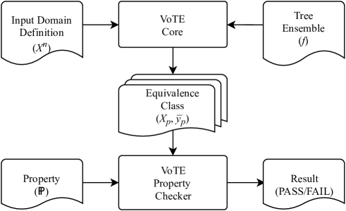
Figure 4: Overview of VoTE.

4.3 Computing Equivalence Classes

There are three distinct tasks being carried out by VoTE Core while computing equivalence classes of a tree ensemble:

• partitioning the input domain of decision trees into disjoint sets,

• exploring all feasible path combinations in the tree ensemble,

• deriving output tuples from leaves.

Path exploration is performed by walking the trees depth-first. The order in which intermediate nodes are considered is described in Section 4.4. When a leaf is hit, the output $\bar{y}_{p}$ for the traversed path combination $p$ is incremented with the value associated with the leaf, and path exploration continues with the next tree. The set of inputs $X_{p}$ is captured by a set of constraints derived from decision functions associated with internal nodes encountered while traversing $p$. When all leaves in a path combination have been processed, an optional post-processing function is applied to $\bar{y}_{p}$, e.g., a division by the number of trees in the case of random forests, and the $\operatorname*{softmax}$ function in the case of a gradient boosting machine classifier (recall the definition of a random forest in Section 2.2 which includes a division, and the use of the softmax function for classifiers in Section 2.5). Finally, the VoTE Property Checker checks if the mappings from $X_{p}$ to $\bar{y}_{p}$ comply with the property $\mathbb{P}$. If the property holds, the next available path combination is traversed, otherwise verification terminates with a “FAIL” and provides the most recent ($X_{p}$, $\bar{y}_{p}$) mapping as a counterexample.

4.4 Node Selection Strategy

Each decision function effectively splits the input domain into smaller pieces throughout the analysis. When a joint evaluation of two decision functions yields an empty set of points, our method concludes an infeasible path combination and continues with the next path combination. One way of improving the performance is to reduce the time spent on analyzing infeasible path combination by discovering them early. Consider the example depicted in Figure 5. When performing the split as illustrated by the dashed line, the left-hand slice $X_{4}$ contains significantly fewer points than the right-hand slice $X_{5}$. Our method is based on the idea that by selecting the child nodes in an order based on the number of points captured by each slice, splits that yield empty sets of points are encountered earlier.

Figure 5: An example used to illustrate our node selection strategy. The dashed line indicates a split of a hyperrectangle into two pieces. Our node selection strategy considers the piece with the least number of points first.

We believe that by choosing the child node which captures the least number of points first, significant performance is to be expected compared to a static selection strategy, e.g., by always selecting the left child first as implemented in previous work [31].

4.5 Approximating Output Bounds

The output of a tree ensemble may be bounded by analyzing each leaf in the collection of trees exactly once. Assuming that all trees are of equal size, the number of leaves in a tree ensemble is $B\cdot 2^{d}$, where $B$ is the number of trees and $d$ the tree depth, thus making the analysis scale linearly with respect to the number of trees.

Definition 6 (Approximate Tree Output Bounds)

Let $t:X^{n}\rightarrow\mathbb{R}^{m}$ be a decision tree with $k$ leaves, and $T=\{t(\bar{x}):\forall\bar{x}\in X^{n}\}$ the image of $t$, i.e., the set of output tuples associated with those leaves. We then approximate the output of $t$ as an interval $[\bar{t}_{\min},\bar{t}_{\max}]$, where

$$\bar{t}_{\min}=(\min\{T_{1,1},\ldots,T_{k,1}\},\ldots,\min\{T_{1,m},\ldots,T_{k,m}\}),$$

$$\bar{t}_{\max}=(\max\{T_{1,1},\ldots,T_{k,1}\},\ldots,\max\{T_{1,m},\ldots,T_{k,m}\}),$$

and $T_{i,j}$ denotes the $j$-th element in the $i$-th output tuple in $T$.

Lemma 1 (Sound Tree Output Approximation)

The approximate tree output bounds $[\bar{t}_{\min},\bar{t}_{\max}]$ of a decision tree $t:X^{n}\rightarrow\mathbb{R}^{m}$ are sound, i.e.,

$$\forall\bar{x}\in X^{n},\bar{t}_{\min}\leq t(\bar{x})\leq\bar{t}_{\max}.$$

Proof 1

For an arbitrary $\bar{x}\in X^{n}$, let $t(\bar{x})=(v_{1},\ldots,v_{m})$. Expansion of $\bar{t}_{\min}\leq t(\bar{x})\leq\bar{t}_{\max}$ then yields

$$\begin{cases}\min\{T_{1,1},\ldots,T_{k,1}\}\leq v_{1}\leq\max\{T_{1,1},\ldots,T_{k,1}\}\\ \vdots\\ \min\{T_{1,m},\ldots,T_{k,m}\}\leq v_{m}\leq\max\{T_{1,m},\ldots,T_{k,m}\}.\end{cases}$$

Since $\bar{x}$ is drawn from the domain of $t$, and $T$ is the image of $t$, then the output scalar $v_{j}$ is captured by $T$. Specifically, $v_{j}\in\bigcup\limits_{i=1}^{k}\{T_{i,j}\}$. Hence, as per the definition of the $\max$ and $\min$ set operators,

$$\forall j\in\{1,\ldots,m\},\min\{T_{1,j},\ldots,T_{k,j}\}\leq v_{j}\leq\max\{T_{1,j},\ldots,T_{k,j}\}.$$

Definition 7 (Approximate Ensemble Output Bounds)

Let $f:X^{n}\rightarrow\mathbb{R}^{m}$ be an ensemble of $B$ trees with a post processing function $p:\mathbb{R}^{m}\rightarrow\mathbb{R}^{m}$, i.e.,

$$f(\bar{x})=p(t_{1}(\bar{x})+\ldots+t_{B}(\bar{x})),$$

where $t_{i}:X^{n}\rightarrow\mathbb{R}^{m}$ is the $i$-th tree in the ensemble. We then approximate the output of $f$ as an interval $[\bar{y}_{\min},\bar{y}_{\max}]$, where

$$\bar{y}_{\min}=p(\bar{t}_{\min_{1}}+\ldots+\bar{t}_{\min_{B}}),$$

$$\bar{y}_{\max}=p(\bar{t}_{\max_{1}}+\ldots+\bar{t}_{\max_{B}}),$$

and $[\bar{t}_{\min_{i}}$, $\bar{t}_{\max_{i}}]$ is the approximate tree output bounds of the $i$-th tree.

Theorem 1 (Sound Ensemble Output Approximation)

The approximate ensemble output bounds
$[\bar{y}_{\min},\bar{y}_{\max}]$ of an ensemble $f:X^{n}\rightarrow\mathbb{R}^{m}$ with a post processing function $p:\mathbb{R}^{m}\rightarrow\mathbb{R}^{m}$ are sound if $p$ is monotonic, i.e.,

$$\forall\bar{x}\in X^{n},\bar{y}_{\min}\leq f(\bar{x})\leq\bar{y}_{\max}.$$

Proof 2

Using Lemma 1, we know that $\forall i\in\{1,\ldots,B\},\forall\bar{x}\in X^{n},t_{i}(\bar{x})\leq\bar{t}_{\max_{i}}$, and that

$$t_{1}(\bar{x})+\ldots+t_{B}(\bar{x})\leq\bar{t}_{\max_{1}}+\ldots+\bar{t}_{\max_{B}}.$$

Since $p$ is monotonic, for $\bar{v}_{1},\bar{v}_{2}\in\mathbb{R}^{m},\bar{v}_{1}\leq\bar{v}_{2}\implies p(\bar{v}_{1})\leq p(\bar{v}_{2})$, it follows that $\forall\bar{x}\in X^{n}$,

$$t_{1}(\bar{x})+\ldots+t_{B}(\bar{x})\leq t_{\max_{1}}+\ldots+t_{\max_{B}}\implies$$

$$p(t_{1}(\bar{x})+\ldots+t_{B}(\bar{x}))\leq p(t_{\max_{1}}+\ldots+t_{\max_{B}})\iff$$

$$f(\bar{x})\leq\bar{y}_{\max}.$$

Analogously, the lower bound $\bar{y}_{\min}$ is also sound.

These output bounds may be used by a property checker to approximate $f$ in, e.g., the plausibility of range property from Section 2.6, assuming that the used post-processing function is monotonic. This assumption holds for random forests since the post-processing function is simply a constant division. Several prominent gradient boosting machines, e.g., CatBoost [24], use the $\operatorname*{softmax}$ function to post-process multiclass classifications, a function which is also known to be monotonic [12].

Note that this approximation technique is sound, but not complete. If property checking does not yield “PASS” with the approximation (see details below), the property $\mathbb{P}$ may still hold, and further analysis of the tree ensemble is required, e.g., by computing all possible equivalence classes (which is exhaustive and precise).

4.6 Implementation

This section presents implementation details of VoTE Core and VoTE Property Checker, aspects that impact accuracy in floating-point computations, and how VoTE can be adapted to tree ensembles with user-defined post-processing functions.

4.6.1 VoTE Core

For efficiency, core features in VoTE are implemented as a library in C, and utilize a pipeline architecture as illustrated by Figure 6 to compute and enumerate equivalence classes.

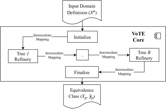
Figure 6: Control flow of equivalence class partitioning in VoTE Core.

The first processing element in the pipeline constructs an intermediate mapping from the entire input domain to an output tuple of zeros. The final processing element applies an optional post-processing function to output tuples, e.g., a division by the number of trees as in the case of a random forest, and the $\operatorname*{softmax}$ function in the case of a gradient boosting machine classifier. In between, there is one refinery element for each tree that splits intermediate mappings into disjoint regions according to decision functions in the trees, and increments the output with values carried by the leaves.

To decouple VoTE from any particular machine learning library, a tree ensemble is loaded into memory by reading a JSON-formatted file from disk. VoTE includes support tools to convert random forests trained by the library scikit-learn [23] and gradient boosting machines trained with CatBoost [24] to this file format.

Currently, VoTE Core includes post-processing functions for random forests and gradient boosting classifiers. Which one to use for a particular problem instance is specified in the JSON file. VoTE can be easily adapted to support additional post-processing functions by simply implementing them inside VoTE Core, or integrating them with a user-defined property checker.

4.6.2 VoTE Property Checker

VoTE includes two pre-defined property checkers which are parameterized and executed from a command-line interface; the plausibility of range property checker, and the robustness property checker.

The plausibility of range property checker first uses the output bound approximation to check for property violations, and resorts to equivalence-class analysis only when a violation is detected when using the approximation.

The robustness property checker checks that all points $X_{r}$ within a hypercube with sides $\epsilon$, centered around a test point $\bar{x}_{t}$, map to the same output. Note that selecting which test points to include in the verification may be problematic. In principle, all points in the input domain should be checked for robustness, but with classifiers, there is always a hyperplane separating two classes from each other, and thus there are always points which violate the robustness property (adjacent to each side of the hyperplane). Hence, the property is only applicable to points at distances greater than $\epsilon$ from any classification boundaries.

VoTE also includes Python bindings for easy prototyping of domain-specific property checkers. Example 2 depicts an implementation of the plausibility of range property that uses these Python bindings to perform sanity checking for a classifier’s output.

Example 2 (Plausibility of Range for a Classifier)

Ensure that the probability of all classes in every prediction is within $[0,1]$.

⬇

import sys

import vote

def plausibility_of_range(mapping, alpha=0, beta=1):

minval = min([mapping.outputs[dim].lower

for dim in range(mapping.nb_outputs)])

maxval = max([mapping.outputs[dim].upper

for dim in range(mapping.nb_outputs)])

return (minval >= alpha) and (maxval <= beta)

e = vote.Ensemble(sys.argv[1]) # load model from disk

assert e.forall(plausibility_of_range)

4.6.3 Computational Accuracy

Implementations of tree ensembles normally approximate real values as floating-point numbers, and thus may suffer from inaccurate computations. In general, VoTE and the software subject to verification must use the same precision on floating-point numbers and prediction function in, e.g., Definition 2 to get a compatible property satisfaction. In this version of VoTE, we use the same representation so that the calculation errors are the same as in the machine learning library scikit-learn [23] and CatBoost [24]. Specifically, we approximate real values as 32-bit floating-point numbers, and implement the prediction functions literally as presented in, e.g., Definition 2, i.e., by first computing the sum of all individual trees, then dividing by the number of trees. Other machine learning libraries may use 64-bit floating-point numbers, and may implement the prediction function differently, e.g.,

$$f(\bar{x})=\sum\limits_{b=1}^{B}\frac{t_{b}(\bar{x})}{B}.$$

This would be easily changeable in VoTE.

5 Case Studies

In this section, we present an evaluation of VoTE on two case studies from the literature where neural networks have been analyzed for compliance with interesting properties. Each case study defines a training set and a test set. We used scikit-learn [23] to train random forests, and CatBoost [24] to train gradient boosting machines. For random forests, all training parameters except the number of trees and maximum tree depth were kept constant and at their default values. When training gradient boosting machines, we also adjusted the learning rate to 0.5 since the default value demonstrated poor accuracy on our case studies. Furthermore, since gradient boosting machines typically use shallower trees than random forests, we used different tree depths and different number of trees for these types of ensembles. In fact, CatBoost is limited to a maximum tree depth of 16.

We evaluated accuracy on each trained model against its test set, i.e., the percentage of samples from the test set where there are no misclassifications, in order to ensure that we were verifying instances that were interesting enough to evaluate. We then developed verification cases for the plausibility of range and robustness against noise properties (from Section 2.6) using VoTE. The time spent on verification was recorded for each trained model as presented below. Next, we evaluated the least-points-first node selection strategy (from Section 4.4) against two baselines on all case studies (always picking the left child first, and always picking the right child first).

Experiments were conducted on a single machine with an Intel Core i5 2500 K CPU and 16 GB RAM. Furthermore, we used a GeForce GTX 1050 Ti GPU with 4 GB of memory to speed up training of gradient boosting machines.

5.1 Vehicle Collision Detection

In this case study, we verified properties of tree ensembles trained to detect collisions between two moving vehicles traveling along curved trajectories at different speeds. Each verified model accepts six input variables, emits two output variables, and contains 20–25 trees with depths between 5–20.

5.1.1 Dataset

We used a simulation tool from Ehlers [9] to generate 30,000 training samples and 3,000 test samples. Unlike neural networks which Ehlers used in his case study, the size of a tree ensemble is limited by the amount of data available during training. Hence, we generated ten times more training data than Ehlers to ensure that sufficient data is available for the size and number of trees assessed in our case study. Each sample contains the relative distance between the two vehicles, the speed and starting direction of the second vehicle, and the rotation speed of both vehicles. Each feature in the dataset is given in normalized form (position, speed, and direction fall in the range $[0,1]$, and rotation speed in the range $[-1,1]$).

5.1.2 Robustness

We verified the robustness against noise for all trained models by defining input regions surrounding each sample in the test set with the robustness margin $\epsilon=0.05$, which amounts to a 5 % change since the data is normalized. Table 1 lists tree ensembles included in the experiment with their maximum tree depth $d$, number of trees $B$, accuracy of the classifications (Accuracy), elapsed time $T$ during verification, and the percentage of samples from the test set where there were no misclassifications within the robustness region (Robustness).

Table 1: Accuracy, robustness, and elapsed verification time (T) of tree ensembles in the vehicle collision detection case study.

Type	$d$	$B$	Accuracy (%)	Robustness (%)	$T$ (s)
RF	10	20	90.4	48.9	56
RF	10	25	90.0	50.3	286
RF	15	20	93.0	34.1	273
RF	15	25	92.9	35.1	1651
RF	20	20	94.2	29.5	367
RF	20	25	94.5	29.6	2520
GB	5	20	93.4	44.5	1
GB	5	25	93.8	40.4	2
GB	10	20	95.5	34.4	26
GB	10	25	95.7	34.0	69
GB	15	20	95.8	34.0	222
GB	15	25	96.0	33.8	511

Increasing the maximum depth of trees increased accuracy on the test set, but reduced the robustness against noise. Adding more trees to a random forest slightly improves its robustness, while gradient boosting machines decreased their robustness against noise as more trees were added. These observations suggest that the models were over-fitted with noiseless examples during training, and thus adding noisy examples to the training set may improve robustness. The elapsed time during verification was significantly less for gradient boosting machines than random forests (using the same parameters). The significant difference in elapsed time between, e.g., gradient boosting machines with $\{d=5,B=20\}$ and $\{d=15,B=25\}$, may seem counter-intuitive at first. However, recall that the theoretical upper limit of the number of path combinations in a tree ensemble is $2^{d\cdot B}$, and that $2^{5\cdot 20}\ll 2^{15\cdot 25}$.

Since our observations suggest that the models were over-fitted, we generated a new training data set which contains 750,000 additional samples with additive noise drawn from the uniform distribution. Specifically, for each sample in the noiseless training data set with an input tuple $\bar{x}$, we added 25 new samples with the input $\bar{x}+\bar{z}$ and the same output, where $\bar{z}$ is a tuple of elements drawn from $\mathcal{U}(-\epsilon,\epsilon)$. We then reran the experiments after training new models on the noisy data set. The results from these experiments are listed in Table 2 in the same format as before.

Table 2: Accuracy, robustness, and elapsed verification time (T) of tree ensembles in the vehicle collision detection case study, trained on a data set with additive random noise.

Type	$d$	$B$	Accuracy (%)	Robustness (%)	$T$ (s)
RF	10	20	89.3	59.4	209
RF	10	25	89.1	60.0	904
RF	15	20	92.4	42.4	2779
RF	15	25	92.2	42.4	12833
RF	20	20	93.6	31.3	7640
RF	20	25	93.7	32.7	53387
GB	5	20	92.7	50.7	2
GB	5	25	93.1	46.2	4
GB	10	20	94.6	35.7	44
GB	10	25	94.7	34.2	142
GB	15	20	94.6	33.3	391
GB	15	25	94.8	32.5	1642

Adding noise to the training data reduced the accuracy with at most 1.2 %, but improved on the robustness against perturbations with up to 10.5 %. More interestingly, models trained on noisy data were more time-consuming to verify compared to those trained on noiseless data, particularly when using random forests. After careful inspection of trees trained on the different data sets, we noticed that random forests trained on the noiseless data contain branches that are shorter than the maximum tree depth. Consequently, there are fewer path combinations in these random forests compared to those trained on the noisy data, which could explain the differing measurements in elapsed verification times.

5.1.3 Node Selection Strategy

Next, we evaluated the least-points-first node selection strategy against the two baseline strategies. Table 3 lists the elapsed verification time for the evaluated models when using the least-points-first node selection strategy ($T$), always selecting the left child first as implemented in the tool VoRF from previous work [31] ($T_{\mathit{VoRF}}$), and always selecting the right child first ($T_{\mathit{right}}$).

Table 3: Elapsed time for different node selection strategies in the vehicle collision detection case study.

Type	$d$	$B$	$T_{\mathit{VoRF}}$ (s)	$T_{\mathit{right}}$ (s)	$T$ (s)
RF	10	20	79	74	56
RF	10	25	422	374	286
RF	15	20	399	441	273
RF	15	25	2351	2457	1651
RF	20	20	930	847	367
RF	20	25	5499	4522	2520
GB	5	20	1	1	1
GB	5	25	3	3	2
GB	10	20	30	31	26
GB	10	25	84	85	69
GB	15	20	265	259	222
GB	15	25	618	616	511

The least-points-first node selection strategy was more effective on random forests than on gradient boosting machines, with speedup factors in the range 1.3–2.5 versus 1.0–1.5, respectively. However, gradient boosting machines were already significantly easier to verify than random forests (with the same number of trees and depth).

5.1.4 Scalability

Next, we assessed the scalability of VoTE Core when the number of trees grows by verifying the trivial property $\mathbb{P}=\mathit{true}$ which accepts all input-output mappings. We implemented this trivial property in a verification case that also counts the number of equivalence classes emitted by VoTE Core. We then executed the verification case for models trained with a maximum tree depth of $d=10$. The recorded number of equivalence classes $C$ for different number of trees $B$ is depicted in Figure 7 on a logarithmic scale.

Figure 7: Number of equivalence classes $C$ on a logarithmic scale from the vehicle collision detection case study for different number of trees $B$ with a depth $d=10$.

The number of equivalence classes increased exponentially as more trees were added, but the magnitude of the growth decreased for each added tree. The number of equivalence classes for large number of trees are significantly smaller than the upper limit of $2^{d\cdot B}$ (which occurs when there are no shared features amongst trees, and thus each path combination yields a distinct equivalence class). Furthermore, the gradient boosting machines consistently yield significantly fewer equivalence classes than random forests, which could explain the differences in verification times we observed between the two types of models (with the same number of trees and depth).

5.1.5 Plausibility of Range

Finally, we verified the plausibility of range property (here ensuring that all predicted probabilities are in the range $[0,1]$). All random forests passed the verification case within fractions of a second thanks to the fast output bound approximation algorithm. For gradient boosting machines however, the output approximations were too conservative; hence we resorted the precise technique. All gradient boosting machines passed the verification case, and the elapsed time during verification for different node selection strategies are listed in Table 4.

Table 4: Elapsed time for different node selection strategies when verifying gradient boosting machines in the vehicle collision detection case study.

$d$	$B$	$T_{\mathit{VoRF}}$ (s)	$T_{\mathit{right}}$ (s)	$T_{\mathit{VoTE}}$ (s)
5	20	2	2	2
5	25	10	10	9
10	20	304	289	260
10	25	1067	1015	917
15	20	3032	3230	2910
15	25	10582	9900	8750

The least-points-first node selection strategy consistently outperformed the two baseline strategies, with speedup factors in the range 1.0–1.2.

5.2 Digit Recognition

In this case study, we verified properties of tree ensembles trained to recognize images of hand-written digits.

5.2.1 Dataset

The MNIST dataset [20] is a collection of hand-written digits commonly used to evaluate machine learning algorithms. The dataset contains 70,000 gray-scale images with a resolution of $28\times 28$ pixels at 8 bpp, encoded as tuples of 784 scalars. We randomized the dataset and split into two subsets; a 85 % training set, and a 15 % test set (a similar split was used in [20]).

5.2.2 Robustness

We defined input regions surrounding each sample in the test set with the robustness margin $\epsilon=1$, which amounts to a 0.5 % lighting change per pixel in a 8 bpp gray-scaled image. Each input region contains $2^{784}$ noisy images, which would be too many for VoTE to handle within a reasonable amount of time. Consequently, we reduced the complexity of the problem significantly by only considering robustness against noise within a sliding window of $5\times 5$ pixels. For a given sample from the test set, noise was added within the $5\times 5$ window, yielding $2^{5\cdot 5}$ noisy images. This operation was then repeated on the original image, but with the window placed at an offset of 1px relative to its previous position. Applying this operation on an entire image yields $2^{5\cdot 5}\cdot(28-5)^{2}\approx 2^{34}$ distinct noisy images per sample from the test set, and about $10^{14}$ noisy images when applied to the entire test set.

Figure 8 depicts one of many examples from the MNIST dataset that were misclassified by the tree ensemble with $B=25$ and $d=10$. Since the added noise is invisible to the naked eye, the noise (a single pixel) is highlighted in red inside the circle.

Figure 8: A misclassified noisy sample from the MNIST dataset.

Table 5 lists tree ensembles included in the experiment with their maximum tree depth $d$, number of trees $B$, accuracy on the test set (Accuracy), elapsed time $T$ during verification, and the percentage of samples from the test set where there were no misclassifications within the robustness region (Robustness).

Table 5: Accuracy and robustness of tree ensembles in the digit recognition case study.

Type	$d$	$B$	Accuracy (%)	Robustness (%)	$T$ (s)
RF	10	20	93.8	75.2	254
RF	10	25	94.2	74.8	1217
RF	15	20	95.8	82.8	436
RF	15	25	96.0	84.0	2141
RF	20	20	96.0	82.3	391
RF	20	25	96.4	83.7	1552
GB	5	75	94.5	60.9	129
GB	5	150	95.3	67.3	301
GB	5	300	95.7	68.6	1551
GB	10	25	94.9	65.8	82
GB	10	50	95.7	73.9	159
GB	10	100	96.3	78.8	486

Increasing the complexity of a tree ensemble slightly increased its accuracy, and significantly increased its robustness against noise. The elapsed time during verification was significantly less for gradient boosting machines than random forests (using the same parameters).

5.2.3 Node Selection Strategy

Next, we evaluated the least-points-first node selection strategy against the two baseline strategies. Table 6 lists the elapsed verification time for the evaluated models when using the least-points-first node selection strategy ($T$), always selecting the left child first as implemented in the tool VoRF from previous work [31] ($T_{\mathit{VoRF}}$), and always selecting the right child first ($T_{\mathit{right}}$).

Table 6: Elapsed time for different child node selection strategies in the digit recognition case study.

Type	$d$	$B$	$T_{\mathit{VoRF}}$ (s)	$T_{\mathit{right}}$ (s)	$T$ (s)
RF	10	20	2009	1093	254
RF	10	25	10724	5386	1217
RF	15	20	4474	1837	436
RF	15	25	23718	8960	2141
RF	20	20	4037	1817	391
RF	20	25	17360	7228	1552
GB	5	75	836	376	129
GB	5	150	2419	848	301
GB	5	300	18829	4717	1551
GB	10	25	442	268	82
GB	10	50	1157	561	159
GB	10	100	5772	1618	486

The effectiveness of our node selection strategy was similar for both random forests and gradient boosting machines, with significant speed up factors in the range 4.2–11.2 and 2.8–12.1, respectively.

5.2.4 Scalability

Next, we assessed the scalability of VoTE Core when the number of trees grows by verifying the trivial property $\mathbb{P}=\mathit{true}$. This was done in a similar way as described in the vehicle collision detection use case presented in Section 5.1.4. We then executed the verification case for all models with a tree depth of $d=10$. Enumerating all possible equivalence classes was intractable for tree ensembles with more than $B=4$ trees. We aborted the experiment after running the verification case with a tree ensembles of $B=5$ for 72 h. Figure 9 depicts the four data points we managed to acquire for the two types of models.

Figure 9: Number of equivalence classes $C$ on a logarithmic scale from the digit recognition case study for different number of trees $B$ with a depth $d=10$.

The number of equivalence classes increased exponentially as more trees were added, without demonstrating any signs of stagnation. The ability to discard infeasible path combinations in a tree ensembles is an essential ingredient to our method. When tree ensembles are trained on high-dimensional data, the number of features shared between trees is relatively low, so it is not surprising that our method experiences combinatorial path explosion.

As described in Section 5.2.2, state explosion was already anticipated when considering robustness to noise when changing arbitrary pixels in the whole state space. This was the underlying reason why the property $\mathbb{P}$ to verify was formulated as robustness to noise when changing pixels within a sliding window of $5\times 5$ pixels, which significantly reduced the search space. This reduction in space was anticipated based on some intuition about the application domain. Not having this intuition may lead to trying to prove properties that are tougher than required, or eliminating a class of applications (e.g., image processing) with long verification times.

5.2.5 Plausibility of Range

Finally, we verified the plausibility of range property (again ensuring that that all predicted probabilities are in the range $[0,1]$). All random forests passed the verification case within fractions of a second thanks to the fast output bound approximation algorithm. For gradient boosting machines however, the output approximations were too conservative. Since the precise technique does not scale well on models trained on high-dimensional data, we were unable to verify the plausibility of range property of gradient boosting machines in this case study.

6 Conclusions and Future Work

In this paper, we proposed a method to formally verify properties of tree ensembles. Our method exploits the fact that several trees make decisions based on a shared subset of the input variables, and thus several path combinations in tree ensembles are infeasible. We implemented the method in a tool called VoTE, and demonstrated its scalability on two case studies.

In the first case study, a collision detection problem with six input variables, we demonstrated that problems with a low-dimensional input space can be verified using our method within a reasonable amount of time. In the second case study, a digit recognition problem with 784 input variables, we demonstrated that our method copes with high-dimensional input space when verifying robustness against noise. But it does so only if the systematically introduced noise does not attempt to exhaustively cover all possibilities. Since the number of shared input variables between trees is low, we observed a combinatorial explosion of paths in the tree ensembles. This combinatorial explosion also appeared when we verified the plausibility of range property of gradient boosting machines where the fast approximation technique was too conservative. However, when verifying the plausibility of range property of random forests, the approximation technique was sufficiently accurate, and verification was completed within seconds.

There exist properties and systems for which formal verification may not be successfully deployed. Conversely, using random sampling for testing robustness may not be acceptable as an argument in a safety assurance case, unless a clear relation between the test samples and the property needed for safety can be mathematically established. Additional work to identify where to apply testing and where formal verification saves time is a useful direction to explore.

For future work, we plan to investigate different tree selection strategies, i.e., strategies that determine in which order trees in an ensemble are analyzed. We also consider combining our approximation technique with our precise technique into an abstraction-refinement scheme. Other directions of work include creating new properties that are meaningful in the context of the problem at hand, e.g., decisive classifications, and applying to use cases where control is involved (and not only sensing).

Acknowledgements

This work was partially supported by the Wallenberg AI, Autonomous Systems and Software Program (WASP) funded by the Knut and Alice Wallenberg Foundation.

References

- Bastani et al. [2018] O. Bastani, Y. Pu, A. Solar-Lezama, Verifiable reinforcement learning via policy extraction, in: Advances in Neural Information Processing Systems (NIPS), 2018, pp. 2494–2504.
- Bastani et al. [2019] O. Bastani, X. Zhang, A. Solar-Lezama, Probabilistic verification of fairness properties via concentration, Proc. ACM Program. Lang. 3 (2019). doi:10.1145/3360544.
- Breiman [1984] L. Breiman, Classification and regression trees, Wadsworth International Group, 1984.
- Breiman [2001] L. Breiman, Random forests, Machine learning 45 (2001) 5–32. doi:10.1023/A:1010933404324.
- Burton et al. [2017] S. Burton, L. Gauerhof, C. Heinzemann, Making the case for safety of machine learning in highly automated driving, in: International Conference on Computer Safety, Reliability, and Security (SAFECOMP), Springer International Publishing, 2017, pp. 5–16. doi:10.1007/978-3-319-66284-8\_1.
- Cheng et al. [2018] C.H. Cheng, G. Nührenberg, C.H. Huang, H. Ruess, Verification of binarized neural networks via inter-neuron factoring, in: R. Piskac, P. Rümmer (Eds.), Verified Software. Theories, Tools, and Experiments (VSTTE), Springer International Publishing, 2018, pp. 279–290.
- DO-333 [2012] DO-333, Formal Methods Supplement to DO-178C and DO-278A, RTCA, Inc., 2012.
- Dutta et al. [2018] S. Dutta, S. Jha, S. Sankaranarayanan, A. Tiwari, Output range analysis for deep feedforward neural networks, in: A. Dutle, C. Muñoz, A. Narkawicz (Eds.), NASA Formal Methods (NFM), Springer International Publishing, 2018, pp. 121–138.
- Ehlers [2017] R. Ehlers, Formal verification of piece-wise linear feed-forward neural networks, in: International Symposium on Automated Technology for Verification and Analysis (ATVA), Springer International Publishing, 2017, pp. 269–286. doi:10.1007/978-3-319-68167-2\_19.
- Esteva et al. [2017] A. Esteva, B. Kuprel, R.A. Novoa, J. Ko, S.M. Swetter, H.M. Blau, S. Thrun, Dermatologist-level classification of skin cancer with deep neural networks, Nature 542 (2017) 115. doi:10.1038/nature21056.
- Friedman [2001] J.H. Friedman, Greedy function approximation: a gradient boosting machine, Annals of statistics (2001) 1189–1232.
- Gao and Pavel [2017] B. Gao, L. Pavel, On the properties of the softmax function with application in game theory and reinforcement learning, arXiv preprint arXiv:1704.00805 (2017).
- Huang et al. [2017] X. Huang, M. Kwiatkowska, S. Wang, M. Wu, Safety verification of deep neural networks, in: R. Majumdar, V. Kunčak (Eds.), Computer Aided Verification (CAV), Springer International Publishing, 2017, pp. 3–29.
- Irsoy et al. [2012] O. Irsoy, O.T. Yıldız, E. Alpaydın, Soft decision trees, in: Proceedings of the 21st International Conference on Pattern Recognition (ICPR), IEEE, 2012, pp. 1819–1822.
- Ivanov et al. [2019] R. Ivanov, J. Weimer, R. Alur, G.J. Pappas, I. Lee, Verisig: verifying safety properties of hybrid systems with neural network controllers, in: Proceedings of the 22th International Conference on Hybrid Systems: Computation and Control, Association for Computing Machinery, 2019, pp. 169–178. doi:10.1145/3302504.3311806.
- Julian et al. [2016] K.D. Julian, J. Lopez, J.S. Brush, M.P. Owen, M.J. Kochenderfer, Policy compression for aircraft collision avoidance systems, in: Digital Avionics Systems Conference (DASC), 2016 IEEE/AIAA 35th, IEEE, 2016, pp. 1–10. doi:10.1109/DASC.2016.7778091.
- Katz et al. [2017] G. Katz, C. Barrett, D.L. Dill, K. Julian, M.J. Kochenderfer, Reluplex: An efficient SMT solver for verifying deep neural networks, in: International Conference on Computer Aided Verification (CAV), Springer International Publishing, 2017, pp. 97–117. doi:10.1007/978-3-319-63387-9\_5.
- Kouvaros and Lomuscio [2018] P. Kouvaros, A. Lomuscio, Formal verification of CNN-based perception systems, arXiv preprint arXiv:1811.11373 (2018).
- Kurd et al. [2007] Z. Kurd, T. Kelly, J. Austin, Developing artificial neural networks for safety critical systems, Neural Computing and Applications 16 (2007) 11–19. doi:10.1007/s00521-006-0039-9.
- LeCun et al. [1998] Y. LeCun, L. Bottou, Y. Bengio, P. Haffner, Gradient-based learning applied to document recognition, Proceedings of the IEEE 86 (1998) 2278–2324. doi:10.1109/5.726791.
- Mirman et al. [2018] M. Mirman, T. Gehr, M. Vechev, Differentiable abstract interpretation for provably robust neural networks, in: Proceedings of the 35th International Conference on Machine Learning (ICML), 2018, pp. 3578–3586.
- Narodytska et al. [2018] N. Narodytska, S. Kasiviswanathan, L. Ryzhyk, M. Sagiv, T. Walsh, Verifying properties of binarized deep neural networks, in: Thirty-Second AAAI Conference on Artificial Intelligence, 2018, pp. 6615–6624.
- Pedregosa et al. [2011] F. Pedregosa, G. Varoquaux, A. Gramfort, V. Michel, B. Thirion, O. Grisel, M. Blondel, P. Prettenhofer, R. Weiss, V. Dubourg, et al., Scikit-learn: Machine learning in Python, Journal of machine learning research 12 (2011) 2825–2830.
- Prokhorenkova et al. [2018] L. Prokhorenkova, G. Gusev, A. Vorobev, A.V. Dorogush, A. Gulin, Catboost: unbiased boosting with categorical features, in: Advances in Neural Information Processing Systems (NIPS), 2018, pp. 6639–6649.
- Pulina and Tacchella [2012] L. Pulina, A. Tacchella, Challenging SMT solvers to verify neural networks, AI Communications 25 (2012) 117–135. doi:10.3233/AIC-2012-0525.
- Russell et al. [2015] S. Russell, D. Dewey, M. Tegmark, Research priorities for robust and beneficial artificial intelligence, AI Magazine 36 (2015) 105–114. doi:10.1609/aimag.v36i4.2577.
- Scheibler et al. [2015] K. Scheibler, L. Winterer, R. Wimmer, B. Becker, Towards verification of artificial neural networks, in: Automatic Verification and Analysis of Complex Systems (MBMV), 2015, pp. 30–40.
- Seshia et al. [2018] S.A. Seshia, X.J. Zhu, A. Krause, S. Jha, Machine Learning and Formal Methods, Dagstuhl Seminar 17351, Schloss Dagstuhl-Leibniz-Zentrum fuer Informatik, 2018. doi:10.4230/DagRep.7.8.55.
- Silver et al. [2016] D. Silver, A. Huang, C.J. Maddison, A. Guez, L. Sifre, G. Van Den Driessche, J. Schrittwieser, I. Antonoglou, V. Panneershelvam, M. Lanctot, et al., Mastering the game of Go with deep neural networks and tree search, Nature 529 (2016) 484–489. doi:10.1038/nature16961.
- Tjeng et al. [2019] V. Tjeng, K.Y. Xiao, R. Tedrake, Evaluating robustness of neural networks with mixed integer programming, in: International Conference on Learning Representations (ICLR), 2019.
- Törnblom and Nadjm-Tehrani [2019] J. Törnblom, S. Nadjm-Tehrani, Formal verification of random forests in safety-critical applications, in: C. Artho, P.C. Ölveczky (Eds.), Formal Techniques for Safety-Critical Systems, Springer International Publishing, 2019, pp. 55–71.
- Wang et al. [2018a] F. Wang, Q. Wang, F. Nie, W. Yu, R. Wang, Efficient tree classifiers for large scale datasets, Neurocomputing 284 (2018a).
- Wang et al. [2018b] S. Wang, K. Pei, J. Whitehouse, J. Yang, S. Jana, Efficient formal safety analysis of neural networks, in: Advances in Neural Information Processing Systems (NIPS), 2018b, pp. 6367–6377.