Solving Dependency Quantified Boolean Formulas
Using Quantifier Localization

Abstract

Dependency quantified Boolean formulas (DQBFs) are a powerful formalism, which subsumes quantified Boolean formulas (QBFs) and allows an explicit specification of dependencies of existential variables on universal variables. Driven by the needs of various applications which can be encoded by DQBFs in a natural, compact, and elegant way, research on DQBF solving has emerged in the past few years. However, research focused on closed DQBFs in prenex form (where all quantifiers are placed in front of a propositional formula), while non-prenex DQBFs have almost not been studied in the literature. In this paper, we provide a formal definition for syntax and semantics of non-closed non-prenex DQBFs and prove useful properties enabling quantifier localization. Moreover, we make use of our theory by integrating quantifier localization into a state-of-the-art DQBF solver. Experiments with prenex DQBF benchmarks, including all instances from the QBFEVAL’18–’20 competitions, clearly show that quantifier localization pays off in this context.

1 Introduction

During the last two decades enormous progress in the solution of quantifier-free Boolean formulas (SAT) has been observed. Nowadays, SAT solving is successfully used in many applications, e. g., in planning [2], automatic test pattern generation [3, 4], and formal verification of hard- and software systems [5, 6, 7]. Motivated by the success of SAT solvers, efforts have been made, e. g., [8, 9, 10, 11], to consider the more general formalism of quantified Boolean formulas (QBFs).

Although QBFs are capable of encoding decision problems in the PSPACE complexity class, they are not powerful enough to succinctly encode many natural and practical problems that involve decisions under partial information. For example, the analysis of games with incomplete information [12], topologically constrained synthesis of logic circuits [13], synthesis of safe controllers [14], synthesis of fragments of linear-time temporal logic (LTL) [15], and verification of partial designs [16, 17] fall into this category and require an even more general formalism, which is known as dependency quantified Boolean formulas (DQBFs) [12].

Unlike QBFs, where an existential variable implicitly depends on all the universal variables preceding its quantification level, DQBFs admit that arbitrary dependency sets are explicitly specified. Essentially, these quantifications with explicit dependency sets correspond to Henkin quantifiers [18]. The semantics of a DQBF can be interpreted from a game-theoretic viewpoint as a game played by one universal player and multiple non-cooperative existential players with incomplete information, each partially observing the moves of the universal player as specified by his/her own dependency set. A DQBF is true if and only if the existential players have winning strategies. This specificity of dependencies allows DQBF encodings to be exponentially more compact than their equivalent QBF counterparts. In contrast to the PSPACE-completeness of QBF, the decision problem of DQBF is NEXPTIME-complete [12].

Driven by the needs of the applications mentioned above, research on DQBF solving has emerged in the past few years, leading to solvers such as iDQ [19], HQS [20, 21, 22], dCAQE [23], iProver [24], and DQBDD [25].

As an example for a DQBF, consider the formula

$$\forall x_{1}\forall x_{2}\exists y_{1}(x_{1})\exists y_{2}(x_{2})\,:\,(x_{1}\wedge x_{2})\equiv(y_{1}\equiv y_{2})$$

from [26]. Here $\forall x_{1}\forall x_{2}\exists y_{1}(x_{1})\exists y_{2}(x_{2})$ is called the quantifier prefix and $(x_{1}\wedge x_{2})\equiv(y_{1}\equiv y_{2})$ the matrix of the DQBF. This DQBF asks whether there are choices for $y_{1}$ only depending on the value of $x_{1}$, denoted $\exists y_{1}(x_{1})$, and for $y_{2}$ only depending on $x_{2}$, denoted $\exists y_{2}(x_{2})$, such that the Boolean formula after the quantifier prefix evaluates to true for all assignments to $x_{1}$ and $x_{2}$. The Boolean formula in turn states that the existential variables $y_{1}$ and $y_{2}$ have to be equal iff $x_{1}$ and $x_{2}$ are true. Since $y_{1}$ can only ‘see’ $x_{1}$ and $y_{2}$ only $x_{2}$, $y_{1}$ and $y_{2}$ ‘cannot coordinate’ to satisfy the constraint. Thus, the formula is false. Now consider a straightforward modification of this DQBF into a QBF with only implicit dependency sets. Changing the quantifier prefix into a QBF quantifier prefix $\forall x_{1}\exists y_{1}\forall x_{2}\exists y_{2}$ means that $y_{1}$ may depend on $x_{1}$, but $y_{2}$ may depend on $x_{1}$ and $x_{2}$. In that case the formula would be true. Changing the prefix into $\forall x_{2}\exists y_{2}\forall x_{1}\exists y_{1}$ has a similar effect.

So far, syntax and semantics of DQBFs have been defined only for closed prenex forms (see for instance [13]), i. e., for DQBFs where all quantifiers are placed in front of the matrix and all variables occurring in the matrix are either universally or existentially quantified. In this paper, we consider quantifier localization for DQBF, which transforms prenex DQBFs into non-prenex DQBFs for more efficient DQBF solving.

Quantifier localization for QBF has been used with great success for image and pre-image computations in the context of sequential equivalence checking and symbolic model checking where it has been called “early quantification”. Here existential quantifiers were moved over AND operations [27, 28, 29, 30]. In [31] the authors consider quantifier localization for QBFs where the matrix is restricted to conjunctive normal form (CNF). They move universal and existential quantifiers over AND operations and propose a method to construct a tree-shaped quantifier structure from a QBF instance with linear quantifier prefix. Moreover, they show how to benefit from this structure in the QBF solving phase. This work has been used and generalized in [32] for a QBF solver based on symbolic quantifier elimination.

To the best of our knowledge, quantifier localization has not been considered for DQBF so far, apart from the seminal theoretical work on DQBF by Balabanov et al. [13], which considers – as a side remark – quantifier localization for DQBF, transforming prenex DQBFs into non-prenex DQBFs. For quantifier localization they gave two propositions. However, a formal definition of the semantics of non-prenex DQBFs was missing in that work and, in addition, the two propositions are not sound, as we will show in our paper.

In this paper, we provide a formal definition of syntax and semantics of non-prenex non-closed DQBFs. The semantics is based on Skolem functions and is a natural generalization of the semantics for closed prenex DQBFs known from the literature. We introduce an alternative constructive definition of the semantics and show that both semantics are equivalent. Then we define rules for transforming DQBFs into equivalent or equisatisfiable DQBFs, which enable the translation of prenex DQBFs into non-prenex DQBFs. The rules are similar to their QBF counterparts, but it turns out that some of them need additional conditions for being sound for DQBF as well. Moreover, the proof techniques are completely different from those for their corresponding QBF counterparts. We provide proofs for all the rules. Finally, we show a method that transforms a prenex DQBF into a non-prenex DQBF based on those rules. It is inspired by the method constructing a tree-shaped quantifier structure from [31] and works for DQBFs with an arbitrary formula (circuit) structure for the matrix. The approach tries to push quantifiers “as deep into the formula” as possible. Whenever a sub-formula fulfills conditions, which we will specify in Section 3, it is processed by symbolic quantifier elimination. When traversing the structure back, quantifiers which could not be eliminated are pulled back into the direction of the root. At the end, a prenex DQBF solver is used for the simplified formula. Experimental results demonstrate the benefits of our method when applied to a set of more than 5000 DQBF benchmarks (including all QBFEVAL’18–’20 competition [33, 34, 35] benchmarks).

The paper is structured as follows: In Section 2 we provide preliminaries needed to understand the paper, including existing transformation rules for QBFs. Section 3 contains the main conceptual results of the paper whereas Section 4 shows how to make use of them algorithmically. Section 5 presents experimental results and Section 6 concludes the paper.

2 Preliminaries

Let $\varphi,\kappa$ be quantifier-free Boolean formulas over the set $V$ of variables and $v\in V$. We denote by $\varphi[\nicefrac{{\kappa}}{{v}}]$ the Boolean formula which results from $\varphi$ by replacing all occurrences of $v$ (simultaneously) by $\kappa$. For a set $V^{\prime}\subseteq V$ we denote by $\mathbf{A}(V^{\prime})$ the set of Boolean assignments for $V^{\prime}$, i. e., $\mathbf{A}(V^{\prime})=\bigl{\{}\mu\,\big{|}\,\mu:V^{\prime}\to\{0,1\}\bigr{\}}$. As usual, for a Boolean assignment $\mu\in\mathbf{A}(V^{\prime})$ and $V^{\prime\prime}\subseteq V^{\prime}$ we denote the restriction of $\mu$ to $V^{\prime\prime}$ by $\mu|_{V^{\prime\prime}}$. For each formula $\varphi$ over $V$, a variable assignment $\mu\in\mathbf{A}(V)$ induces a truth value $0$ or $1$ of $\varphi$, which we call $\mu(\varphi)$. If $\mu(\varphi)=1$ for all $\mu\in\mathbf{A}(V)$, then $\varphi$ is a tautology. In this case we write $\vDash\varphi$.

A Boolean function with the set of input variables $V$ is a mapping $f:\mathbf{A}(V)\to\{0,1\}$. The set of Boolean functions over $V$ is denoted by $\mathbb{F}_{V}$. The support $\operatorname{supp}(f)$ of a function $f\in\mathbb{F}_{V}$ is defined by $\operatorname{supp}(f)\colonequals\{v\in V\;|\;\exists\mu,\mu^{\prime}\in\mathbf{A}(V)\mbox{ with }\mu(w)=\mu^{\prime}(w)\,\text{ for all }w\in V\setminus\{v\}\mbox{ and }f(\mu)\neq f(\mu^{\prime})\}$. $\operatorname{supp}(f)$ is the set of variables from $V$ on which $f$ “really depends”. The constant zero and constant one function are $\mathbf{0}$ and $\mathbf{1}$, respectively. $\mathrm{ITE}$ denotes the if-then-else operator, i. e., $\mathrm{ITE}(f,g,h)=(f\land g)\lor(\neg f\land h)$.

A function $f:\mathbf{A}(V)\to\{0,1\}$ is monotonically increasing (decreasing) in $v\in V$, if $f(\mu)\leq f(\mu^{\prime})$ ($f(\mu^{\prime})\leq f(\mu)$) for all assignments $\mu,\mu^{\prime}\in\mathbf{A}(V)$ with $\mu(w)=\mu^{\prime}(w)$ for all $w\in V\setminus\{v\}$ and $\mu(v)\leq\mu^{\prime}(v)$.

A quantifier-free Boolean formula $\varphi$ over $V$ defines a Boolean function $f_{\varphi}:\mathbf{A}(V)\to\{0,1\}$ by $f_{\varphi}(\mu)\colonequals\mu(\varphi)$. When clear from the context, we do not differentiate between quantifier-free Boolean formulas and the corresponding Boolean functions, e. g., if $\varphi$ is a Boolean formula representing $f_{\varphi}$, we write $\varphi[\nicefrac{{v^{\prime}}}{{v}}]$ for the Boolean function where the input variable $v$ is replaced by a (new) input variable $v^{\prime}$.

Now we consider Boolean formulas with quantifiers. The usual definition for a closed prenex DQBF is given as follows:

Definition 1 (Closed prenex DQBF).

Let $V=\{x_{1},\ldots,x_{n},\allowbreak y_{1},\ldots,y_{m}\}$ be a set of Boolean variables. A dependency quantified Boolean formula (DQBF) $\psi$ over $V$ has the form

$$\psi\colonequals\forall x_{1}\forall x_{2}\ldots\forall x_{n}\exists y_{1}(D_{y_{1}})\exists y_{2}(D_{y_{2}})\ldots\exists y_{m}(D_{y_{m}}):\varphi$$

where $D_{y_{i}}\subseteq\{x_{1},\ldots,x_{n}\}$ for $i=1,\ldots,m$ is the dependency set of $y_{i}$, and $\varphi$ is a quantifier-free Boolean formula over $V$, called the matrix of $\psi$.

We denote the set of universal variables of $\psi$ by $V^{\forall}_{\psi}=\{x_{1},\ldots,x_{n}\}$ and its set of existential variables by $V^{\exists}_{\psi}=\{y_{1},\ldots,y_{m}\}$. The former part of $\psi$, $\forall x_{1}\forall x_{2}\ldots\forall x_{n}\allowbreak\exists y_{1}(D_{y_{1}})\exists y_{2}(D_{y_{2}})\ldots\exists y_{m}(D_{y_{m}})$, is called its prefix. Sometimes we abbreviate this prefix as $Q$ such that $\psi=Q:\varphi$.

The semantics of closed prenex DQBFs is given as follows:

Definition 2 (Semantics of closed prenex DQBF).

Let $\psi$ be a DQBF with matrix $\varphi$ as above. $\psi$ is satisfiable iff there are functions $s_{y_{i}}:\mathbf{A}(D_{y_{i}})\to\{0,1\}$ for $1\leq i\leq m$ such that replacing each $y_{i}$ by (a Boolean formula for) $s_{y_{i}}$ turns $\varphi$ into a tautology. Then the functions $(s_{y_{i}})_{i=1,\ldots,m}$ are called Skolem functions for $\psi$.

A DQBF is a QBF, if its dependency sets satisfy certain conditions:

Definition 3 (Closed prenex QBF).

Let $V=\{x_{1},\ldots,x_{n},\allowbreak y_{1},\ldots,y_{m}\}$ be a set of Boolean variables. A quantified Boolean formula (QBF) (more precisely, a closed QBF in prenex normal form) $\psi$ over $V$ is given by $\psi\colonequals\forall X_{1}\exists Y_{1}\ldots\forall X_{k}\exists Y_{k}:\varphi$, where $k\geq 1$, $X_{1},\ldots,X_{k}$ is a partition of the universal variables $\{x_{1},\ldots,x_{n}\}$, $Y_{1},\ldots,Y_{k}$ is a partition of the existential variables $\{y_{1},\ldots,y_{m}\}$, $X_{i}\neq\emptyset$ for $i=2,\ldots,k$, and $Y_{j}\neq\emptyset$ for $j=1,\ldots,k-1$, and $\varphi$ is a quantifier-free Boolean formula over $V$.

A QBF can be seen as a DQBF where the dependency sets are linearly ordered. A QBF $\psi\colonequals\forall X_{1}\exists Y_{1}\ldots\forall X_{k}\exists Y_{k}:\varphi$ is equivalent to the DQBF $\psi^{\prime}\colonequals\forall x_{1}\ldots\forall x_{n}\exists y_{1}(D_{y_{1}})\ldots$ $\exists y_{m}(D_{y_{m}}):\varphi$ with $D_{y_{i}}=\bigcup_{j=1}^{\ell}X_{j}$ where $Y_{\ell}$ is the unique set with $y_{i}\in Y_{\ell}$, $1\leq\ell\leq k$, $1\leq i\leq m$.

Quantifier localization for QBF is based on the following theorem (see, e. g., [31]) which can be used to transform prenex QBFs into equivalent or equisatisfiable non-prenex QBFs (where the quantifiers are not necessarily placed before the matrix). Two QBFs $\psi_{1}$ and $\psi_{2}$ are equisatisfiable ($\psi_{1}\approx\psi_{2}$), when $\psi_{1}$ is satisfiable iff $\psi_{2}$ is satisfiable.

Theorem 1.

Let $\mathbin{\diamond}\in\{{\land},{\lor}\}$, let $\mathcal{Q}\in\{\exists,\forall\}$, $\overline{\mathcal{Q}}=\exists$, if $\mathcal{Q}=\forall$ and $\overline{\mathcal{Q}}=\forall$ otherwise. Let $V^{\mathrm{free,supp}}_{\psi}$ be the set of all variables occurring in $\psi$ which are not bound by a quantifier. The following holds for all QBFs:

$$\neg(\mathcal{Q}x:\psi) \quad\approx\quad\overline{\mathcal{Q}}x:(\neg\psi)$$ (1a)

$$\mathcal{Q}x:\psi \quad\approx\quad\psi,\;\text{ if }x\notin V^{\mathrm{free,supp}}_{\psi}$$ (1b)

$$\forall x:(\psi_{1}\land\psi_{2}) \quad\approx\quad(\forall x:\psi_{1})\land(\forall x:\psi_{2})$$ (1c)

$$\exists x:(\psi_{1}\lor\psi_{2}) \quad\approx\quad(\exists x:\psi_{1})\lor(\exists x:\psi_{2})$$ (1d)

$$\mathcal{Q}x:(\psi_{1}\mathbin{\diamond}\psi_{2}) \quad\approx\quad\bigl{(}\psi_{1}\mathbin{\diamond}(\mathcal{Q}x:\psi_{2})\bigr{)},\;\text{ if }x\notin V^{\mathrm{free,supp}}_{\psi_{1}}$$ (1e)

$$\mathcal{Q}x_{1}\,\mathcal{Q}x_{2}:\psi \quad\approx\quad\mathcal{Q}x_{2}\,\mathcal{Q}x_{1}:\psi$$ (1f)

3 Non-Closed Non-Prenex DQBFs

3.1 Syntax and Semantics

In this section, we define syntax and semantics of non-prenex DQBFs. Since the syntax definition is recursive, we need non-closed DQBFs as well.

$$\begin{array}[]{@{}cccccc}\hline\cr\hline\cr\textnormal{No.}&\textnormal{Rule}&&V^{\exists}_{\cdot}&V^{\forall}_{\cdot}&V^{\mathrm{free,supp}}_{\cdot}\\ \hline\cr 1&\dfrac{v\in V}{v\in\Phi^{\mathrm{ncnp}}}&&\emptyset&\emptyset&\{v\}\\[8.53581pt] 2&\dfrac{v\in V}{\neg v\in\Phi^{\mathrm{ncnp}}}&&\emptyset&\emptyset&\{v\}\\[5.69054pt] 3&\dfrac{\varphi_{1}\in\Phi^{\mathrm{ncnp}}\qquad\varphi_{2}\in\Phi^{\mathrm{ncnp}}\qquad\eqref{eq:disjoint}}{(\varphi_{1}\land\varphi_{2})\in\Phi^{\mathrm{ncnp}}}&&V^{\exists}_{\varphi_{1}}\mathbin{\dot{\cup}}V^{\exists}_{\varphi_{2}}&V^{\forall}_{\varphi_{1}}\mathbin{\dot{\cup}}V^{\forall}_{\varphi_{2}}&V^{\mathrm{free,supp}}_{\varphi_{1}}\cup V^{\mathrm{free,supp}}_{\varphi_{2}}\\[11.38109pt] 4&\dfrac{\varphi_{1}\in\Phi^{\mathrm{ncnp}}\qquad\varphi_{2}\in\Phi^{\mathrm{ncnp}}\qquad\eqref{eq:disjoint}}{(\varphi_{1}\lor\varphi_{2})\in\Phi^{\mathrm{ncnp}}}&&V^{\exists}_{\varphi_{1}}\mathbin{\dot{\cup}}V^{\exists}_{\varphi_{2}}&V^{\forall}_{\varphi_{1}}\mathbin{\dot{\cup}}V^{\forall}_{\varphi_{2}}&V^{\mathrm{free,supp}}_{\varphi_{1}}\cup V^{\mathrm{free,supp}}_{\varphi_{2}}\\[14.22636pt] 5&\dfrac{\varphi\in\Phi^{\mathrm{ncnp}}\qquad v\in V^{\mathrm{free}}_{\varphi}\qquad D_{v}\subseteq V\setminus\bigl{(}V_{\varphi}^{Q}\mathbin{\dot{\cup}}\{v\}\bigr{)}}{\exists v(D_{v}):\varphi^{-v}\in\Phi^{\mathrm{ncnp}}}&&V^{\exists}_{\varphi}\mathbin{\dot{\cup}}\{v\}&V^{\forall}_{\varphi}&V^{\mathrm{free,supp}}_{\varphi}\setminus\{v\}\\[11.38109pt] 6&\dfrac{\varphi\in\Phi^{\mathrm{ncnp}}\qquad v\in V^{\mathrm{free}}_{\varphi}}{\forall v:\varphi\in\Phi^{\mathrm{ncnp}}}&&V^{\exists}_{\varphi}&V^{\forall}_{\varphi}\mathbin{\dot{\cup}}\{v\}&V^{\mathrm{free,supp}}_{\varphi}\setminus\{v\}\\ \hline\cr\hline\cr\end{array}$$

where ($\ast$ ‣ 1) refers to the formula

$$\Big{(}V_{\varphi_{1}}^{Q}\cup V^{\mathrm{free,supp}}_{\varphi_{1}}\cup\bigcup_{y\in V^{\exists}_{\varphi_{1}}}D_{y}\Big{)}\cap V_{\varphi_{2}}^{Q}=\emptyset\quad\land\quad\Big{(}V_{\varphi_{2}}^{Q}\cup V^{\mathrm{free,supp}}_{\varphi_{2}}\cup\bigcup_{y\in V^{\exists}_{\varphi_{2}}}D_{y}\Big{)}\cap V_{\varphi_{1}}^{Q}=\emptyset\,. \ast$$ ()

Figure 1: Rules defining the syntax of non-prenex non-closed DQBFs in negation normal form.

Definition 4 (Syntax).

Let $V$ be a finite set of Boolean variables. Let $\varphi^{-v}$ result from $\varphi$ by removing $v$ from the dependency sets of all existential variables in $\varphi$.

The set $\Phi^{\mathrm{ncnp}}$ of non-closed non-prenex DQBFs in negation normal form (NNF) over $V$, the existential and universal variables as well as the free variables in their support are defined by the rules given in Figure 1. As usual, $\Phi^{\mathrm{ncnp}}$ is defined to be the smallest set satisfying those rules.

$V^{\exists}_{\psi}$ is the set of existential variables of $\psi$, $V^{\forall}_{\psi}$ the set of universal variables of $\psi$, and $V^{\mathrm{free,supp}}_{\psi}$ the set of free variables in the support of $\psi$. $V_{\psi}\colonequals V^{\exists}_{\psi}\mathbin{\dot{\cup}}V^{\forall}_{\psi}\mathbin{\dot{\cup}}V^{\mathrm{free,supp}}_{\psi}$ is the set of variables occurring in $\psi$, $V_{\psi}^{Q}\colonequals V^{\exists}_{\psi}\mathbin{\dot{\cup}}V^{\forall}_{\psi}$ is the set of quantified variables of $\psi$, and $V^{\mathrm{free}}_{\psi}\colonequals V\setminus V_{\psi}^{Q}$ is the set of free variables of $\psi$.

Remark 1.

For the sake of simplicity, we assume in Definition 4 that variables are either free or bound by some quantifier, but not both, and that no variable is quantified more than once. Every formula that violates this assumption can easily be brought into the required form by renaming variables. We restrict ourselves to NNF, since prenex DQBFs are not syntactically closed under negation [13]. For closed prenex DQBFs the (quantifier-free) matrix can be simply transformed into NNF by applying De Morgan’s rules and omitting double negations (exploiting that $x\equiv\neg\neg x$) at the cost of a linear blow-up of the formula.

For two DQBFs $\psi_{1},\psi_{2}$ we write $\psi_{1}\sqsubseteq\psi_{2}$ if $\psi_{1}$ is a subformula of $\psi_{2}$.

Definition 5 (Skolem function candidates).

For a DQBF $\psi$ over variables $V$ in NNF, we define a Skolem function candidate as a mapping from existential and free variables to functions over universal variables $s:V^{\mathrm{free}}_{\psi}\mathbin{\dot{\cup}}V^{\exists}_{\psi}\to\mathbb{F}_{V^{\forall}_{\psi}}$ with

1. $\operatorname{supp}\bigl{(}s(v)\bigr{)}=\emptyset$ for all $v\in V^{\mathrm{free}}_{\psi}$, i. e., $s(v)\in\{\mathbf{0},\mathbf{1}\}$, and

2. $\operatorname{supp}\bigl{(}s(v)\bigr{)}\subseteq\bigl{(}D_{v}\cap V^{\forall}_{\psi}\bigr{)}$ for all $v\in V^{\exists}_{\psi}$.

$\mathbb{S}_{\psi}$ is the set of all such Skolem function candidates.

That means, $\mathbb{S}_{\psi}$ is the set of all Skolem function candidates satisfying the constraints imposed by the dependency sets of the existential and free variables.

Notation 1.

Given $s\in\mathbb{S}_{\psi}$ for a DQBF $\psi\in\Phi^{\mathrm{ncnp}}$, we write $s(\psi)$ for the formula that results from $\psi$ by replacing each variable $v$ for which $s$ is defined by $s(v)$ and omitting all quantifiers from $\psi$, i. e., $s(\psi)$ is a quantifier-free Boolean formula, containing only variables from $V^{\forall}_{\psi}$.

Definition 6 (Semantics of DQBFs in NNF).

Let $\psi\in\Phi^{\mathrm{ncnp}}$ be a DQBF over variables $V$. We define the semantics $\llbracket\psi\rrbracket$ of $\psi$ as follows:

$$\llbracket\psi\rrbracket\colonequals\bigl{\{}s\in\mathbb{S}_{\psi}\,\big{|}\,\vDash s(\psi)\bigr{\}}=\bigl{\{}s\in\mathbb{S}_{\psi}\,\big{|}\,\forall\mu\in\mathbf{A}(V^{\forall}_{\psi}):\mu\bigl{(}s(\psi)\bigr{)}=1\bigr{\}}.$$

$\psi$ is satisfiable if $\llbracket\psi\rrbracket\neq\emptyset$; otherwise we call it unsatisfiable. The elements of $\llbracket\psi\rrbracket$ are called Skolem functions for $\psi$.

The semantics $\llbracket\psi\rrbracket$ of $\psi$ is the subset of $\,\mathbb{S}_{\psi}$ such that for all $s\in\llbracket\psi\rrbracket$ we have: Replacing each free or existential variable $v\in V^{\mathrm{free}}_{\psi}\mathbin{\dot{\cup}}V^{\exists}_{\psi}$ with a Boolean expression for $s(v)$ turns $\psi$ into a tautology.

Example 1.

Consider the DQBF

$$\psi\colonequals\forall x_{1}\forall x_{2}:\Bigl{(}\bigl{(}x_{1}\equiv x_{2}\bigr{)}\vee\bigl{(}\exists y_{1}(x_{2}):(x_{1}\not\equiv y_{1})\bigr{)}\Bigr{)}$$

over the set of variables $\{x_{1},x_{2},y_{1}\}$. $y_{1}$ with dependency set $\{x_{2}\}$ is the only existential variable in $\psi$ and there are no free variables. Thus $\mathbb{S}_{\psi}=\{y_{1}\mapsto\mathbf{0},y_{1}\mapsto\mathbf{1},y_{1}\mapsto x_{2},y_{1}\mapsto\neg x_{2}\}$. It is easy to see that $s\colonequals y_{1}\mapsto x_{2}$ is a Skolem function for $\psi$, since $\vDash s(\psi)=\bigl{(}(x_{1}\equiv x_{2})\vee(x_{1}\not\equiv x_{2})\bigr{)}$, and that the other Skolem function candidates do not define Skolem functions.

Remark 2.

For closed prenex DQBFs the semantics defined here obviously coincides with the usual semantics as specified in Definition 2 if we transform the (quantifier-free) matrix into NNF first.

Remark 3.

A (non-prenex) DQBF $\psi$ is a (non-prenex) QBF if every existential variable depends on all universal variables in whose scope it is (and possibly on free variables as well).

The following theorem provides a constructive characterization of the semantics of a DQBF.

Theorem 2.

The set $\llbracket\psi\rrbracket$ for a DQBF $\psi$ over variables $V$ in NNF can be characterized recursively as follows:

$$\llbracket v\rrbracket =\bigl{\{}s\in\mathbb{S}_{v}\,\big{|}\,s(v)=\mathbf{1}\bigr{\}}\text{ for }v\in V_{\psi},$$ (2a)

$$\llbracket\neg v\rrbracket =\bigl{\{}s\in\mathbb{S}_{\neg v}\,\big{|}\,s(v)=\mathbf{0}\bigr{\}}\text{ for }v\in V_{\psi},$$ (2b)

$$\llbracket(\varphi_{1}\land\varphi_{2})\rrbracket =\bigl{\{}s\in\mathbb{S}_{\varphi_{1}\land\varphi_{2}}\,\big{|}\,s_{|V^{\mathrm{free}}_{\varphi_{1}}\mathbin{\dot{\cup}}V^{\exists}_{\varphi_{1}}}\in\llbracket\varphi_{1}\rrbracket\land s_{|V^{\mathrm{free}}_{\varphi_{2}}\mathbin{\dot{\cup}}V^{\exists}_{\varphi_{2}}}\in\llbracket\varphi_{2}\rrbracket\bigr{\}},$$ (2c)

$$\llbracket(\varphi_{1}\lor\varphi_{2})\rrbracket =\bigl{\{}s\in\mathbb{S}_{\varphi_{1}\lor\varphi_{2}}\,\big{|}\,s_{|V^{\mathrm{free}}_{\varphi_{1}}\mathbin{\dot{\cup}}V^{\exists}_{\varphi_{1}}}\in\llbracket\varphi_{1}\rrbracket\lor s_{|V^{\mathrm{free}}_{\varphi_{2}}\mathbin{\dot{\cup}}V^{\exists}_{\varphi_{2}}}\in\llbracket\varphi_{2}\rrbracket\bigr{\}},$$ (2d)

$$\llbracket\exists v(D_{v}):\varphi^{-v}\rrbracket =\llbracket\varphi^{-v}\rrbracket,$$ (2e)

$$\llbracket\forall v:\varphi\rrbracket =\Bigl{\{}t\in\mathbb{S}_{\forall v:\varphi}\,\Big{|}\,\exists s_{0},s_{1}\in\llbracket\varphi\rrbracket:s_{0}(v)=\mathbf{0}\land s_{1}(v)=\mathbf{1}\;\land$$ (2f)

$$\qquad\forall w\in V^{\mathrm{free}}_{\forall v:\varphi}:t(w)=s_{0}(w)=s_{1}(w)\;\land$$

$$\qquad\forall w\in V^{\exists}_{\forall v:\varphi},v\notin D_{w}:t(w)=s_{0}(w)=s_{1}(w)\;\land$$

$$\qquad\forall w\in V^{\exists}_{\forall v:\varphi},v\in D_{w}:t(w)=\mathrm{ITE}\bigl{(}v,\ s_{1}(w),\ s_{0}(w)\bigr{)}\Bigr{\}}$$

For the proof as well as for the following example, we denote the semantics defined in Definition 6 by $\llbracket\psi\rrbracket_{D}$ (i. e., $\llbracket\psi\rrbracket_{D}=\{s\in\mathbb{S}_{\psi}\,|\,\vDash s(\psi)\}$) and the set that is characterized by Theorem 2 by $\llbracket\psi\rrbracket_{T}$.

Proof.

$\llbracket\psi\rrbracket_{D}=\llbracket\psi\rrbracket_{T}$ is shown by induction on the structure of $\psi$, for details we refer to A. ∎

The following example illustrates the recursive characterization of Theorem 2 (and again the recursive Definition 4).

Example 2.

Let us consider the DQBF

$$\psi\colonequals\forall x_{1}\forall x_{2}:\Bigl{(}\bigl{(}x_{1}\equiv x_{2}\bigr{)}\lor\bigl{(}\exists y_{1}(x_{2}):(x_{1}\not\equiv y_{1})\bigr{)}\Bigr{)}$$

over the set of variables $\{x_{1},x_{2},y_{1}\}$ from Example 1 again. We compute $\llbracket\psi\rrbracket_{T}$ recursively.

As an abbreviation for $\bigl{(}(\neg x_{1}\land y_{1})\lor(x_{1}\land\neg y_{1})\bigr{)}$, $(x_{1}\not\equiv y_{1})$ is a DQBF based on rules 1–4 of Definition 4 with $V^{\exists}_{x_{1}\not\equiv y_{1}}=V^{\forall}_{x_{1}\not\equiv y_{1}}=\emptyset$, $V^{\mathrm{free,supp}}_{x_{1}\not\equiv y_{1}}=\{x_{1},y_{1}\}$, $V^{\mathrm{free}}_{x_{1}\not\equiv y_{1}}=\{x_{1},x_{2},y_{1}\}$. With Theorem 2, (2a)–(2d) we get $\llbracket x_{1}\not\equiv y_{1}\rrbracket_{T}=\bigl{\{}s:\{x_{1},x_{2},y_{1}\}\to\mathbb{F}_{\emptyset}\;\big{|}\;s(y_{1})\neq s(x_{1})\bigr{\}}$.

For $\psi^{\prime}\colonequals\bigl{(}\exists y_{1}(x_{2}):(x_{1}\not\equiv y_{1})\bigr{)}$, we obtain by rule 5: $V^{\forall}_{\psi^{\prime}}=\emptyset$, $V^{\exists}_{\psi^{\prime}}=\{y_{1}\}$, $V^{\mathrm{free,supp}}_{\psi^{\prime}}=\{x_{1}\}$. $V^{\mathrm{free}}_{\psi^{\prime}}=\{x_{1},x_{2}\}$. According to Theorem 2, (2e) we have $\llbracket\exists y_{1}(x_{2}):(x_{1}\not\equiv y_{1})\rrbracket_{T}=\llbracket x_{1}\not\equiv y_{1}\rrbracket_{T}$.

Similarly we obtain $\llbracket x_{1}\equiv x_{2}\rrbracket_{T}=\bigl{\{}s:\{x_{1},x_{2},y_{1}\}\to\mathbb{F}_{\emptyset}\;\big{|}\;s(x_{1})=s(x_{2})\bigr{\}}$.

Then, for $\psi^{\prime\prime}\colonequals\bigl{(}\bigl{(}x_{1}\equiv x_{2}\bigl{)}\vee\bigl{(}\exists y_{1}(x_{2}):(x_{1}\not\equiv y_{1})\bigr{)}\bigr{)}$ we have $V^{\forall}_{\psi^{\prime\prime}}=\emptyset$, $V^{\exists}_{\psi^{\prime\prime}}=\{y_{1}\}$, $V^{\mathrm{free,supp}}_{\psi^{\prime\prime}}=V^{\mathrm{free}}_{\psi^{\prime\prime}}=\{x_{1},x_{2}\}$, and by Theorem 2, (2d) $\llbracket\psi^{\prime\prime}\rrbracket_{T}=\bigl{\{}s:\{x_{1},x_{2},y_{1}\}\to\mathbb{F}_{\emptyset}\;\bigr{|}\;\bigl{(}s(x_{1}),s(x_{2}),s(y_{1})\bigr{)}\in\{(\mathbf{0},\mathbf{0},\mathbf{0}),(\mathbf{0},\mathbf{0},\mathbf{1}),(\mathbf{0},\mathbf{1},\mathbf{1}),(\mathbf{1},\mathbf{0},\mathbf{0}),(\mathbf{1},\mathbf{1},\mathbf{0}),(\mathbf{1},\mathbf{1},\mathbf{1})\}\bigr{\}}$.

Now we consider $\forall x_{2}:\psi^{\prime\prime}$. $V^{\forall}_{\forall x_{2}:\psi^{\prime\prime}}=\{x_{2}\}$. $V^{\exists}_{\forall x_{2}:\psi^{\prime\prime}}=\{y_{1}\}$, $V^{\mathrm{free,supp}}_{\forall x_{2}:\psi^{\prime\prime}}=V^{\mathrm{free}}_{\forall x_{2}:\psi^{\prime\prime}}=\{x_{1}\}$. We use $\eqref{th:semantics:forall}$ to construct $\llbracket\forall x_{2}:\psi^{\prime\prime}\rrbracket_{T}$. In principle, there are three possible choices $s_{0}\in\llbracket\psi^{\prime\prime}\rrbracket_{T}$ with $s_{0}(x_{2})=\mathbf{0}$ and three possible choices $s_{1}\in\llbracket\psi^{\prime\prime}\rrbracket_{T}$ with $s_{1}(x_{2})=\mathbf{1}$. Due to the constraint $s_{0}(x_{1})=s_{1}(x_{1})$ in the third line of $\eqref{th:semantics:forall}$, there remain only four possible combinations $s^{(1)}_{0},s^{(1)}_{1},\ldots,s^{(4)}_{0},s^{(4)}_{1}$:

• $\bigl{(}s^{(1)}_{0}(x_{1}),s^{(1)}_{0}(x_{2}),s^{(1)}_{0}(y_{1})\bigr{)}=(\mathbf{0},\mathbf{0},\mathbf{0})$,
  $\bigl{(}s^{(1)}_{1}(x_{1}),s^{(1)}_{1}(x_{2}),s^{(1)}_{1}(y_{1})\bigr{)}=(\mathbf{0},\mathbf{1},\mathbf{1})$, leading to
  $t^{(1)}(x_{1})=\mathbf{0}$, $t^{(1)}(y_{1})=\mathrm{ITE}\bigl{(}x_{2},s^{(1)}_{1}(y_{1}),s^{(1)}_{0}(y_{1})\bigr{)}=\mathrm{ITE}(x_{2},\mathbf{1},\mathbf{0})=x_{2}$,

• $\bigl{(}s^{(2)}_{0}(x_{1}),s^{(2)}_{0}(x_{2}),s^{(2)}_{0}(y_{1})\bigr{)}=(\mathbf{0},\mathbf{0},\mathbf{1})$,
  $\bigl{(}s^{(2)}_{1}(x_{1}),s^{(2)}_{1}(x_{2}),s^{(2)}_{1}(y_{1})\bigr{)}=(\mathbf{0},\mathbf{1},\mathbf{1})$, leading to
  $t^{(2)}(x_{1})=\mathbf{0}$, $t^{(2)}(y_{1})=\mathrm{ITE}\bigl{(}x_{2},s^{(2)}_{1}(y_{1}),s^{(2)}_{0}(y_{1})\bigr{)}=\mathrm{ITE}(x_{2},\mathbf{1},\mathbf{1})=\mathbf{1}$,

• $\bigl{(}s^{(3)}_{0}(x_{1}),s^{(3)}_{0}(x_{2}),s^{(3)}_{0}(y_{1})\bigr{)}=(\mathbf{1},\mathbf{0},\mathbf{0})$,
  $\bigl{(}s^{(3)}_{1}(x_{1}),s^{(3)}_{1}(x_{2}),s^{(3)}_{1}(y_{1})\bigr{)}=(\mathbf{1},\mathbf{1},\mathbf{0})$, leading to
  $t^{(3)}(x_{1})=\mathbf{1}$, $t^{(3)}(y_{1})=\mathrm{ITE}\bigl{(}x_{2},s^{(3)}_{1}(y_{1}),s^{(3)}_{0}(y_{1})\bigr{)}=\mathrm{ITE}(x_{2},\mathbf{0},\mathbf{0})=\mathbf{0}$,

• $\bigl{(}s^{(4)}_{0}(x_{1}),s^{(4)}_{0}(x_{2}),s^{(4)}_{0}(y_{1})\bigr{)}=(\mathbf{1},\mathbf{0},\mathbf{0})$,
  $\bigl{(}s^{(4)}_{1}(x_{1}),s^{(4)}_{1}(x_{2}),s^{(4)}_{1}(y_{1})\bigr{)}=(\mathbf{1},\mathbf{1},\mathbf{1})$, leading to
  $t^{(4)}(x_{1})=\mathbf{1}$, $t^{(4)}(y_{1})=\mathrm{ITE}\bigl{(}x_{2},s^{(4)}_{1}(y_{1}),s^{(4)}_{0}(y_{1})\bigr{)}=\mathrm{ITE}(x_{2},\mathbf{1},\mathbf{0})=x_{2}$.

Altogether, $\llbracket\forall x_{2}:\psi^{\prime\prime}\rrbracket_{T}=\{t^{(1)},t^{(2)},t^{(3)},t^{(4)}\}$.

Finally, for $\psi=\forall x_{1}\forall x_{2}:\psi^{\prime\prime}$ we have $V^{\forall}_{\psi}=\{x_{1},x_{2}\}$, $V^{\exists}_{\psi}=\{y_{1}\}$, $V^{\mathrm{free,supp}}_{\psi}=V^{\mathrm{free}}_{\psi}=\emptyset$. For the choice of $s_{0}$ and $s_{1}$ in (2f) we need $s_{0}(x_{1})=\mathbf{0}$, $s_{1}(x_{1})=\mathbf{1}$ and, due to $x_{1}\notin D_{y_{1}}$, $s_{0}(y_{1})=s_{1}(y_{1})$ (see the third line of (2f)). Thus, the only possible choice is $s_{0}\colonequals t^{(1)}$ and $s_{1}\colonequals t^{(4)}$; $t(y_{1})\colonequals x_{2}$ is the only possible Skolem function for $\psi$. This result agrees with the Skolem function computed using Definition 6 in Example 1.

3.2 Equivalent and Equisatisfiable Non-Closed Non-Prenex DQBFs

Now we define rules for replacing DQBFs by equivalent and equisatisfiable ones. We start with the definition of equivalence and equisatisfiability:

Definition 7 (Equivalence and equisatisfiability).

Let $\psi_{1},\psi_{2}\in\Phi^{\mathrm{ncnp}}$ be DQBFs over $V$. We call them equivalent (written $\psi_{1}\equiv\psi_{2}$) if $\llbracket\psi_{1}\rrbracket=\llbracket\psi_{2}\rrbracket$; they are equisatisfiable (written $\psi_{1}\approx\psi_{1}$) if $\llbracket\psi_{1}\rrbracket=\emptyset\Leftrightarrow\llbracket\psi_{2}\rrbracket=\emptyset$ holds.

Now we prove Theorem 3, which is the DQBF counterpart to Theorem 1 for QBF.

Theorem 3.

Let $\mathbin{\diamond}\in\{{\land},{\lor}\}$ and all formulas occurring on the left- and right-hand sides of the following rules be DQBFs in $\Phi^{\mathrm{ncnp}}$ over the same set $V$ of variables. We assume that $x^{\prime}$ and $y^{\prime}$ are fresh variables, which do not occur in $\varphi$, $\varphi_{1}$, and $\varphi_{2}$. The following equivalences and equisatifiabilities hold for all DQBFs in NNF.

$$\exists y(D_{y}):\varphi \quad\equiv\quad\varphi$$ (3a)

$$\forall x:\varphi \quad\approx\quad\varphi^{-x}\quad\text{ if }x\notin V_{\varphi}$$ (3b)

$$\forall x:\varphi \quad\equiv\quad\varphi[\nicefrac{{0}}{{x}}]\land\varphi[\nicefrac{{1}}{{x}}]\quad\text{ if }V^{\forall}_{\varphi}=V^{\exists}_{\varphi}=\emptyset$$ (3c)

$$\exists y(D_{y}):\varphi \quad\approx\quad\varphi[\nicefrac{{0}}{{y}}]\lor\varphi[\nicefrac{{1}}{{y}}]\quad\text{ if }V^{\forall}_{\varphi}=V^{\exists}_{\varphi}=\emptyset$$ (3d)

$$\forall x:(\varphi_{1}\land\varphi_{2}) \quad\approx\quad\bigl{(}\forall x:\varphi_{1}\bigr{)}\land\bigl{(}\forall x^{\prime}:\varphi_{2}[\nicefrac{{x^{\prime}}}{{x}}]\bigr{)}$$ (3e)

$$\forall x:(\varphi_{1}\land\varphi_{2}) \quad\approx\quad\bigl{(}\varphi_{1}^{-x}\land(\forall x:\varphi_{2})\bigr{)}\quad\text{ if }x\notin V_{\varphi_{1}}$$ (3f)

$$\forall x:(\varphi_{1}\mathbin{\diamond}\varphi_{2}) \quad\equiv\quad\bigl{(}\varphi_{1}\mathbin{\diamond}(\forall x:\varphi_{2})\bigr{)}\quad\text{ if }x\notin V_{\varphi_{1}}\text{ and }x\notin D_{y}\text{ for all }y\in V^{\exists}_{\varphi_{1}}$$ (3g)

$$\exists y(D_{y}):(\varphi_{1}\lor\varphi_{2}) \quad\approx\quad\bigl{(}\exists y(D_{y}):\varphi_{1}\bigr{)}\lor\bigl{(}\exists y^{\prime}(D_{y}):\varphi_{2}[\nicefrac{{y^{\prime}}}{{y}}]\bigr{)}$$ (3h)

$$\exists y(D_{y}):(\varphi_{1}\mathbin{\diamond}\varphi_{2}) \quad\equiv\quad\bigl{(}\varphi_{1}\mathbin{\diamond}(\exists y(D_{y}):\varphi_{2})\bigr{)}\quad\text{ if }y\notin V_{\varphi_{1}}$$ (3i)

$$\exists y_{1}(D_{y_{1}})\,\exists y_{2}(D_{y_{2}}):\varphi \quad\equiv\quad\exists y_{2}(D_{y_{2}})\,\exists y_{1}(D_{y_{1}}):\varphi$$ (3j)

$$\forall x_{1}\,\forall x_{2}:\varphi \quad\equiv\quad\forall x_{2}\,\forall x_{1}:\varphi$$ (3k)

$$\forall x\,\exists y(D_{y}):\varphi \quad\equiv\quad\exists y(D_{y})\,\forall x:\varphi\quad\text{ if }x\notin D_{y}.$$ (3l)

Note that the duality of $\exists$ and $\forall$ under negation as in QBF ($\exists\varphi\equiv\neg\forall\neg\varphi$) does not hold for DQBF as DQBFs are not syntactically closed under negation [13].

Example 3.

We give an example that shows that – in contrast to (1e) of Theorem 1 for QBF – the condition $x\notin D_{y}$ for all $y\in V^{\exists}_{\varphi_{1}}$ is really needed in (3g) if $\mathbin{\diamond}=\lor$. We consider the satisfiable DQBF $\psi\colonequals\forall x_{1}\forall x_{2}:\bigl{(}(x_{1}\equiv x_{2})\vee(\exists y_{1}(x_{2}):(x_{1}\not\equiv y_{1}))\bigr{)}$ from Example 1 again. First of all, neglecting the above condition, we could transform $\psi$ into $\psi^{\prime}\colonequals\forall x_{1}:\bigl{(}(\forall x_{2}:(x_{1}\equiv x_{2}))\vee(\exists y_{1}(x_{2}):(x_{1}\not\equiv y_{1}))\bigr{)}$, which is not well-formed according to Definition 4. However, by renaming $x_{2}$ into $x^{\prime}_{2}$ in the dependency set of $y_{1}$ we would arrive at a well-formed DQBF $\psi^{\prime\prime}\colonequals\forall x_{1}:\bigl{(}(\forall x_{2}:(x_{1}\equiv x_{2}))\vee(\exists y_{1}(x^{\prime}_{2}):(x_{1}\not\equiv y_{1}))\bigr{)}$. According to Definition 5 the only possible Skolem function candidates for $y_{1}$ in $\psi^{\prime\prime}$ are $\mathbf{0}$ and $\mathbf{1}$. It is easy to see that neither inserting $\mathbf{0}$ nor $\mathbf{1}$ for $y_{1}$ turns $\psi^{\prime\prime}$ into a tautology, thus $\psi^{\prime\prime}$ is unsatisfiable and therefore neither equivalent to nor equisatisfiable with $\psi$.

Whereas the proof of Theorem 1 for QBF is rather easy using the equisatisfiabilities $\exists y:\varphi\approx\varphi[\nicefrac{{0}}{{y}}]\lor\varphi[\nicefrac{{1}}{{y}}]$ and $\forall x:\varphi\approx\varphi[\nicefrac{{0}}{{x}}]\land\varphi[\nicefrac{{1}}{{x}}]$, the proof of Theorem 3 is more involved. We provide a detailed proof in B.

It is also important to note that some of the rules in Theorem 3 establish equivalences and some establish equisatisfiabilities only. Whereas this might seem to be negligible if we are only interested in the question whether a formula is satisfiable or not, it turns out to be essential in the context of Section 4 where we replace subformulas by equivalent or equisatisfiable formulas. Replacing a subformula of a formula $\psi$ by an equisatisfiable subformula does not necessarily preserve satisfiability / unsatisfiability. This observation is trivially true already for pure propositional logic (e. g., $x_{1}$ is equisatisfiable with $x_{1}\lor x_{2}$, but $x_{1}\land\neg x_{1}$ is not equisatisfiable with $(x_{1}\lor x_{2})\land\neg x_{1}$). Here we show a more complex example for DQBFs:

Example 4 (label=ex:counter).

Let us consider the DQBF $\psi\colonequals\exists y(\emptyset):\bigl{(}(x\land y)\lor(\neg x\land\neg y)\bigr{)}$, which is, according to (3h), equisatisfiable with $\psi^{\prime}\colonequals\bigl{(}\exists y(\emptyset):(x\land y)\bigr{)}\lor\bigl{(}\exists y^{\prime}(\emptyset):(\neg x\land\neg y^{\prime})\bigr{)}$. $\forall x:\psi$ is unsatisfiable, since for the choice $s(y)=\mathbf{0}$ we have $s(\forall x:\psi)\equiv\neg x$ and for the choice $s(y)=\mathbf{1}$ we have $s(\forall x:\psi)\equiv x$, i. e., for both possible choices for the Skolem function candidates we do not obtain a tautology. However, $\forall x:\psi^{\prime}$ is satisfiable by $s(y)=\mathbf{1}$ and $s(y^{\prime})=\mathbf{0}$.

It is easy to see that situations like in Example LABEL:ex:counter do not occur when we replace equivalent subformulas:

Theorem 4.

Let $\psi$ be a DQBF and $\psi_{1}\sqsubseteq\psi$ be a subformula of $\psi$. Let $\psi_{2}$ be a DQBF that is equivalent to $\psi_{1}$, $V^{\exists}_{\psi_{1}}=V^{\exists}_{\psi_{2}}$, and each existential variable $y$ has the same dependency set in $\psi_{2}$ as in $\psi_{1}$. Then the DQBF $\psi^{\prime}\colonequals\psi[\nicefrac{{\psi_{2}}}{{\psi_{1}}}]$, which results from replacing $\psi_{1}$ by $\psi_{2}$, is equivalent to $\psi$.

Proof (Sketch) 1.

The proof easily follows from the fact that the set of Skolem functions is identical for equivalent subformulas and from the recursive characterization of the semantics of DQBFs in Theorem 2. If the existential variables in $\psi_{1}$ and $\psi_{2}$ as well as their dependency sets are identical, then the same holds for all $\psi^{\prime}_{1}\sqsubseteq\psi$ and $\psi^{\prime}_{2}\sqsubseteq\psi^{\prime}$ with $\psi_{1}^{\prime}\not\sqsubseteq\psi_{1}$ and $\psi_{2}^{\prime}\not\sqsubseteq\psi_{2}$. We make use of this condition in part (2f) of the inductive proof that shows $\psi\equiv\psi^{\prime}$. Assume $\psi_{1}\ \sqsubseteq\ \forall v:\varphi$. In part (2f), free and existential variables of $\forall v:\varphi$ (resp. of $\forall v:\varphi[\nicefrac{{\psi_{2}}}{{\psi_{1}}}]$) are handled differently and therefore it is not enough to inductively assume that the Skolem functions for $\varphi$ and $\varphi[\nicefrac{{\psi_{2}}}{{\psi_{1}}}]$ are identical, but existential / free variables should also not have “changed their type”. Moreover, existential variables with different dependency sets are handled differently (see last two lines of (2f)), so we also have to assume that the dependency set of each existential variable $y$ in $\psi_{1}$ is the same as its dependency set in $\psi_{2}$. ∎

Remark 4.

Theorem 4 says that it is safe to apply rules (3c), (3g), (3i), (3j), (3k), and (3l) to subformulas as well. Theorem 4 does not imply this for rule (3a), since the sets of existential variables of the left-hand side formula and the right-hand side formula are different.

Since we are still interested in obtaining equisatisfiable formulas by replacing equisatisfiable subformulas, we need to have a closer look at the rules (3a), (3b), (3d), (3e), (3f) and (3h). Example LABEL:ex:counter already shows that we will not be able to achieve our goal in all cases without considering additional conditions.

We start with rule (3a). With the restriction $y\notin V_{\varphi}$ rule (3a) can simply be generalized to subformulas:

Theorem 5.

Let $\psi\in\Phi^{\mathrm{ncnp}}$ be a DQBF over $V$ and let $\exists y(D_{y}):\varphi\ \sqsubseteq\ \psi$ be a subformula of $\psi$ with $y\notin V_{\varphi}$. Then $\psi\approx\psi^{\prime}$ where $\psi^{\prime}$ results from $\psi$ by replacing the subformula $\exists y(D_{y}):\varphi$ by $\varphi$.

Proof.

For each $s\in\llbracket\psi^{\prime}\rrbracket$ we have $s\in\llbracket\psi\rrbracket$ and $\vDash s(\psi^{\prime})$ implies $\vDash s(\psi)$.

Now assume $\llbracket\psi\rrbracket\neq\emptyset$ and $s\in\llbracket\psi\rrbracket$ with $\vDash s(\psi)$. Define $s^{\prime}\in\llbracket\psi^{\prime}\rrbracket$ by $s^{\prime}(y)\colonequals c$ for some $c\in\{\mathbf{0},\mathbf{1}\}$ and $s^{\prime}(v)\colonequals s(v)$ for $v\neq y$. Since $y\notin V_{\varphi}$, the only occurrence of $y$ in $\psi$ is in $\exists y(D_{y})$ due to the rules in Definition 4 and there is no occurrence of $y$ in $\psi^{\prime}$, i. e., $s(\psi)=s^{\prime}(\psi^{\prime})$. Thus $\vDash s(\psi)$ implies $\vDash s^{\prime}(\psi^{\prime})$. ∎

Next we consider rule (3b). Although this rule establishes equisatisfiability only, it may be generalized to the replacement of subformulas:

Theorem 6.

Let $\psi\in\Phi^{\mathrm{ncnp}}$ be a DQBF and let $\forall x:\varphi\ \sqsubseteq\ \psi$ be a subformula of $\psi$ with $x\notin V_{\varphi}$. Then $\psi\approx\psi^{\prime}$ where $\psi^{\prime}$ results from $\psi$ by replacing the subformula $\forall x:\varphi$ by $\varphi^{-x}$.

Proof.

If $\llbracket\psi^{\prime}\rrbracket\neq\emptyset$, then for each $s\in\llbracket\psi^{\prime}\rrbracket$ with $\vDash s(\psi^{\prime})$ we also have $\vDash s(\psi)$ and $s\in\llbracket\psi\rrbracket$. $s$ is a Skolem function candidate for $\psi$ as well, since the supports of the Skolem function candidates for $\psi$ cannot be more restricted than those for $\psi^{\prime}$.

Now assume $\llbracket\psi\rrbracket\neq\emptyset$ and $s\in\llbracket\psi\rrbracket$. Choose $s^{\prime}$ with $s^{\prime}(v)\colonequals s(v)[\nicefrac{{c}}{{x}}]$ for all existential variables $v\in V^{\exists}_{\varphi}$ for an arbitrary constant $c\in\{0,1\}$ and $s^{\prime}(v)\colonequals s(v)$ otherwise. It is clear that $s^{\prime}$ is a Skolem function candidate for $\psi^{\prime}$. Now consider an arbitrary assignment $\mu^{\prime}\in\mathbf{A}(V^{\forall}_{\psi^{\prime}})$. Choose $\mu\in\mathbf{A}(V^{\forall}_{\psi})$ by $\mu(v)\colonequals\mu^{\prime}(v)$ for all $v\in V^{\forall}_{\psi^{\prime}}$ and $\mu(x)\colonequals c$. Because of $x\notin V_{\varphi}$, $x$ occurs in $s(\psi)$ only in Skolem functions. Therefore $\mu^{\prime}\bigl{(}s^{\prime}(\psi^{\prime})\bigr{)}=\mu\bigl{(}s(\psi)\bigr{)}$ and $\mu^{\prime}\bigl{(}s^{\prime}(\psi^{\prime})\bigr{)}=1$, since $s(\psi)$ is a tautology. This proves that $s^{\prime}(\psi^{\prime})$ is a tautology as well and $\llbracket\psi^{\prime}\rrbracket\neq\emptyset$. ∎

Next, we look into rule (3d). Theorem 7 is a variant of this rule which is suitable for replacements of subformulas. Here we have the first situation that we need additional conditions for the proof to go through in the more general context of replacing subformulas. Theorem 7 is strongly needed for our algorithm taking advantage of quantifier localization. It shows that, under certain conditions, we can do symbolic quantifier elimination for non-prenex DQBFs as it is known from QBFs:

Theorem 7.

Let $\psi\in\Phi^{\mathrm{ncnp}}$ be a DQBF and let $\exists y(D_{y}):\varphi\ \sqsubseteq\ \psi$ be a subformula of $\psi$ such that $V^{\forall}_{\varphi}=V^{\exists}_{\varphi}=\emptyset$ and $V_{\varphi}\subseteq D_{y}\cup V^{\mathrm{free}}_{\psi}\cup\{v\in V^{\exists}_{\psi}\;|\;D_{v}\subseteq D_{y}\}$. Then $\psi\approx\psi^{\prime}$ where $\psi^{\prime}$ results from $\psi$ by replacing the subformula $\exists y(D_{y}):\varphi$ by $\varphi[\nicefrac{{0}}{{y}}]\lor\varphi[\nicefrac{{1}}{{y}}]$.

The proof of Theorem 7 is somewhat involved and uses results from [36].

Proof (Sketch) 2.

We show equisatisfiability by proving that $\llbracket\psi^{\prime}\rrbracket\neq\emptyset$ implies $\llbracket\psi\rrbracket\neq\emptyset$ and vice versa.

First assume that there is a Skolem function $s^{\prime}\in\llbracket\psi^{\prime}\rrbracket$ with $\vDash s^{\prime}(\psi^{\prime})$. We define $s\in\mathbb{S}_{\psi}$ by $s(v)\colonequals s^{\prime}(v)$ for all $v\in V^{\exists}_{\psi^{\prime}}\cup V^{\mathrm{free}}_{\psi^{\prime}}\setminus\{y\}$ and $s(y)\colonequals s^{\prime}(\varphi[\nicefrac{{1}}{{y}}])$. The fact that $s\in\mathbb{S}_{\psi}$ follows from the restriction that $\varphi$ contains only variables from $D_{y}\cup V^{\mathrm{free}}_{\psi}\cup\{v\in V^{\exists}_{\psi}\;|\;D_{v}\subseteq D_{y}\}$, i. e., $\operatorname{supp}\bigl{(}s(y)\bigr{)}=\operatorname{supp}\bigl{(}s^{\prime}(\varphi[\nicefrac{{1}}{{y}}])\bigr{)}\subseteq D_{y}$. $\vDash s(\psi)$ follows by some rewriting from a result in [36] proving that quantifier elimination can be done by composition, i. e., $\varphi[\nicefrac{{\varphi[\nicefrac{{1}}{{y}}]}}{{y}}]$ is equivalent to $\varphi[\nicefrac{{0}}{{y}}]\lor\varphi[\nicefrac{{1}}{{y}}]$.

Now assume $s\in\llbracket\psi\rrbracket$ with $\vDash s(\psi)$ and define $s^{\prime}$ just by removing $y$ from the domain of $s$. In a first step we change $s$ into $s^{\prime\prime}$ by replacing $s(y)$ with $s^{\prime\prime}(y)\colonequals s^{\prime}(\varphi)[\nicefrac{{1}}{{y}}]$. We conclude $\vDash s^{\prime\prime}(\psi)$ from [36] and monotonicity properties of $\psi$ in negation normal form. In a second step we use [36] again to show that $s^{\prime\prime}(\psi)$ is equivalent to $s^{\prime}(\psi^{\prime})$. Thus finally $\vDash s^{\prime}(\psi^{\prime})$. The detailed proof can be found in C.∎

The generalization of rule (3e) to replacements of subformulas is formulated in Theorem 8. Here we do not need any additional conditions:

Theorem 8.

Let $\psi\in\Phi^{\mathrm{ncnp}}$ be a DQBF and let $\psi_{1}\colonequals\forall x:(\varphi_{1}\land\varphi_{2})\ \sqsubseteq\ \psi$ be a subformula of $\psi$. Then $\psi\approx\psi^{\prime}$ where $\psi^{\prime}$ results from $\psi$ by replacing the subformula $\psi_{1}$ by $\psi_{2}\colonequals\bigl{(}\forall x:\varphi_{1}\bigr{)}\land\bigl{(}\forall x^{\prime}:\varphi_{2}[\nicefrac{{x^{\prime}}}{{x}}]\bigr{)}$.

Before proving Theorem 8, we consider a lemma which will be helpful for the proofs of Theorems 8, 9, and 10.

Lemma 1.

Let $\varphi_{1}\sqsubseteq\varphi$ be quantifier-free Boolean formulas such that $\varphi_{1}$ is not in the scope of any negation from $\varphi$. Let $\varphi^{\prime}\colonequals\varphi[\nicefrac{{\varphi_{2}}}{{\varphi_{1}}}]$ be the Boolean formula resulting from the replacement of $\varphi_{1}$ by the quantifier-free Boolean formula $\varphi_{2}$ and let $\mu\in\mathbf{A}(V_{\varphi}\cup V_{\varphi^{\prime}})$. If $\mu(\varphi)=1$ and $\mu(\varphi^{\prime})=0$, then $\mu(\varphi_{1})=1$ and $\mu(\varphi_{2})=0$.

Proof.

By assumptions, $\varphi_{1}$ is only in the scope of conjunctions and disjunctions. Due to monotonicity of conjunctions and disjunctions we have $\mu(\varphi[\nicefrac{{0}}{{\varphi_{1}}}])\leq\mu(\varphi[\nicefrac{{1}}{{\varphi_{1}}}])$.

Moreover, by construction, we have $\varphi^{\prime}[\nicefrac{{0}}{{\varphi_{2}}}]=\varphi[\nicefrac{{0}}{{\varphi_{1}}}]$ and $\varphi^{\prime}[\nicefrac{{1}}{{\varphi_{2}}}])=\varphi[\nicefrac{{1}}{{\varphi_{1}}}]$. Further, $\mu(\varphi)=\mu(\varphi[\nicefrac{{c}}{{\varphi_{1}}}])$ if $\mu(\varphi_{1})=c\in\{0,1\}$, and $\mu(\varphi^{\prime})=\mu(\varphi^{\prime}[\nicefrac{{c}}{{\varphi_{2}}}])$ if $\mu(\varphi_{2})=c\in\{0,1\}$.

$\mu(\varphi_{1})=\mu(\varphi_{2})$ is not possible, since we assumed $\mu(\varphi)=1$ and $\mu(\varphi^{\prime})=0$, i. e., $\mu(\varphi)\neq\mu(\varphi^{\prime})$. From $\mu(\varphi_{1})=0$ and $\mu(\varphi_{2})=1$ we could conclude $\mu(\varphi)=\mu(\varphi[\nicefrac{{0}}{{\varphi_{1}}}])\leq\mu(\varphi[\nicefrac{{1}}{{\varphi_{1}}}])=\mu(\varphi^{\prime}[\nicefrac{{1}}{{\varphi_{2}}}])=\mu(\varphi^{\prime})$, which also contradicts $\mu(\varphi)=1$ and $\mu(\varphi^{\prime})=0$. ∎

Proof (Sketch) 3 (Theorem 8).

The proof of Theorem 8 uses Lemma 1 to lift rule (3e) to the more general case of replacements of subformulas. It is easy, but rather technical, and can be found in D.∎

The next theorem shows that rule (3f) can also be generalized to replacements of subformulas without needing additional conditions.

Theorem 9.

Let $\psi\in\Phi^{\mathrm{ncnp}}$ be a DQBF and let $\psi_{1}\colonequals\forall x:(\varphi_{1}\land\varphi_{2})\ \sqsubseteq\ \psi$ be a subformula of $\psi$ with $x\notin V_{\varphi_{1}}$. Then $\psi\approx\psi^{\prime}$ where $\psi^{\prime}$ results from $\psi$ by replacing the subformula $\psi_{1}$ by $\psi_{2}\colonequals\bigl{(}\varphi_{1}^{-x}\land(\forall x:\varphi_{2})\bigr{)}$.

Proof.

The proof easily follows from Theorem 8 and Theorem 6. By Theorem 8, $\psi\approx\psi^{\prime\prime}$ with $\psi^{\prime\prime}\colonequals\psi[\nicefrac{{\psi_{3}}}{{\psi_{1}}}]$ and $\psi_{3}\colonequals\bigl{(}\forall x^{\prime}:\varphi_{1}[\nicefrac{{x^{\prime}}}{{x}}]\bigr{)}\land\bigl{(}\forall x:\varphi_{2}\bigr{)}$. Since $x\notin V_{\varphi_{1}}$, we have $x^{\prime}\notin V_{\varphi_{1}[\nicefrac{{x^{\prime}}}{{x}}]}$, and due to Theorem 6 $\psi^{\prime\prime}\approx\psi^{\prime\prime\prime}$ with $\psi^{\prime\prime\prime}\colonequals\psi[\nicefrac{{\psi_{4}}}{{\psi_{1}}}]$ and $\psi_{4}\colonequals\varphi_{1}[\nicefrac{{x^{\prime}}}{{x}}]^{-x^{\prime}}\land\bigl{(}\forall x:\varphi_{2}\bigr{)}$. Because of $\varphi_{1}[\nicefrac{{x^{\prime}}}{{x}}]^{-x^{\prime}}=\varphi_{1}^{-x}$ we have $\psi_{4}=\psi_{2}$ and thus $\psi\approx\psi^{\prime}$. ∎

Finally, in case of rule (3h) we need non-trivial additional restrictions to preserve satisfiability / unsatisfiability of DQBFs where a subformula $\exists y(D_{y}):(\varphi_{1}\lor\varphi_{2})$ is replaced by $\bigl{(}\exists y(D_{y}):\varphi_{1}\bigr{)}\lor\bigl{(}\exists y^{\prime}(D_{y}):\varphi_{2}[y^{\prime}/y]\bigr{)}$ (or vice versa).

Theorem 10.

Let $\psi\in\Phi^{\mathrm{ncnp}}$ be a DQBF and let $\psi_{1}\colonequals\exists y(D_{y}):(\varphi_{1}\vee\varphi_{2})\sqsubseteq\psi$ be a subformula of $\psi$. Further, let

$$V^{\forall,\mathrm{occ}}_{\varphi_{1}} \colonequals\Big{[}(V^{\forall}_{\psi}\cap V_{\varphi_{1}})\cup\bigcup_{v\in V^{\exists}_{\psi}\cap V_{\varphi_{1}}}(V^{\forall}_{\psi}\cap D_{v})\Big{]}\setminus D_{y},$$

$$V^{\forall,\mathrm{occ}}_{\varphi_{2}} \colonequals\Big{[}(V^{\forall}_{\psi}\cap V_{\varphi_{2}})\cup\bigcup_{v\in V^{\exists}_{\psi}\cap V_{\varphi_{2}}}(V^{\forall}_{\psi}\cap D_{v})\Big{]}\setminus D_{y},$$

$$V^{\forall,\mathrm{occ}}_{\psi\setminus\psi_{1}} \colonequals\Big{[}V^{\forall}_{\psi[\nicefrac{{0}}{{\psi_{1}}}]}\cup\bigcup_{v\in V^{\exists}_{\psi[\nicefrac{{0}}{{\psi_{1}}}]}}(V^{\forall}_{\psi}\cap D_{v})\Big{]}\,.$$

If $V^{\forall,\mathrm{occ}}_{\varphi_{1}}\cap V^{\forall,\mathrm{occ}}_{\varphi_{2}}=\emptyset$ and $V^{\forall,\mathrm{occ}}_{\varphi_{1}}\cap V^{\forall,\mathrm{occ}}_{\psi\setminus\psi_{1}}=\emptyset$ (or $V^{\forall,\mathrm{occ}}_{\varphi_{2}}\cap V^{\forall,\mathrm{occ}}_{\psi\setminus\psi_{1}}=\emptyset$), then $\psi\approx\psi^{\prime}$ where $\psi^{\prime}\colonequals\psi[\nicefrac{{\psi_{2}}}{{\psi_{1}}}]$ results from $\psi$ by replacing $\psi_{1}$ by $\psi_{2}\colonequals(\exists y(D_{y}):\varphi_{1})\vee(\exists y^{\prime}(D_{y}):\varphi_{2}[\nicefrac{{y^{\prime}}}{{y}}])$ with $y^{\prime}$ being a fresh variable.

$V^{\forall,\mathrm{occ}}_{\varphi_{1}}$ ($V^{\forall,\mathrm{occ}}_{\varphi_{2}}$) is the set of all universal variables occurring in $\varphi_{1}$ ($\varphi_{2}$) or in dependency sets of existential variables occurring in $\varphi_{1}$ ($\varphi_{2}$), reduced by the dependency set $D_{y}$ of $y$. $V^{\forall,\mathrm{occ}}_{\psi\setminus\psi_{1}}$ is the set of universal variables occurring in $\psi$ outside the subformula $\psi_{1}$ or in dependency sets of existential variables occurring in $\psi$ outside the subformula $\psi_{1}$. In the proof we use that $V^{\forall,\mathrm{occ}}_{\varphi_{1}}\cap V^{\forall,\mathrm{occ}}_{\varphi_{2}}=\emptyset$ implies that – after replacing existential variables by Skolem functions – $\varphi_{1}$ and $\varphi_{2}$ do not share universal variables other than those from $D_{y}$.

Before we present the proof of Theorem 10, we consider two examples to motivate that it is necessary to add the conditions in the theorem.

Example 5 (continues=ex:counter).

The first example is again the formula $\forall x\exists y(\emptyset):\bigl{(}(x\land y)\lor(\neg x\land\neg y)\bigr{)}$, which showed that rule (3h) cannot be always applied for replacing subformulas without changing the satisfiability of the formula. We now demonstrate that one of the conditions from Theorem 10 does indeed not hold for this formula. Using the same notation as in Theorem 10 we have $\psi_{1}\colonequals\exists y(\emptyset):\bigl{(}(x\land y)\lor(\neg x\land\neg y)\bigr{)}$ with $\varphi_{1}\colonequals(x\land y)$ and $\varphi_{2}\colonequals(\neg x\land\neg y)$. Then $V^{\forall,\mathrm{occ}}_{\varphi_{1}}=V^{\forall,\mathrm{occ}}_{\varphi_{2}}=\{x\}$, which means that the condition $V^{\forall,\mathrm{occ}}_{\varphi_{1}}\cap V^{\forall,\mathrm{occ}}_{\varphi_{2}}=\emptyset$ is not fulfilled and Theorem 10 cannot be applied.

To show that for the correctness of the theorem it is also needed to add condition $V^{\forall,\mathrm{occ}}_{\varphi_{1}}\cap V^{\forall,\mathrm{occ}}_{\psi\setminus\psi_{1}}=\emptyset$ (or $V^{\forall,\mathrm{occ}}_{\varphi_{2}}\cap V^{\forall,\mathrm{occ}}_{\psi\setminus\psi_{1}}=\emptyset$), we give another example:

Example 6 (label=ex:counter2).

Let $\psi_{1}\colonequals\exists y(\emptyset):\bigl{(}(x_{1}\land y)\lor(x_{2}\land\neg y)\bigr{)}$ be a DQBF with $\varphi_{1}\colonequals(x_{1}\land y)$ and $\varphi_{2}\colonequals(x_{2}\land\neg y)$. Let $\psi_{2}\colonequals\bigl{(}\exists y(\emptyset):(x_{1}\land y)\lor\exists y^{\prime}(\emptyset):(x_{2}\land\neg y^{\prime})\bigr{)}$ be the DQBF that results from $\psi_{1}$ by applying rule (3h). Formula $\psi\colonequals\forall x_{1}\forall x_{2}:\psi_{1}\lor(\neg x_{1}\land\neg x_{2})$ is then unsatisfiable, because for $s_{0}(y)=\mathbf{0}$ we have $s_{0}(\psi)\equiv x_{2}\lor(\neg x_{1}\land\neg x_{2})$ and for $s_{1}(y)=\mathbf{1}$ we have $s_{1}(\psi)\equiv x_{1}\lor(\neg x_{1}\land\neg x_{2})$, i. e., for both possible choices for the Skolem function candidates we do not obtain a tautology. However, formula $\psi^{\prime}\colonequals\forall x_{1}\forall x_{2}:\psi_{2}\lor(\neg x_{1}\land\neg x_{2})$ is satisfiable by $s(y)=\mathbf{1}$ and $s(y^{\prime})=\mathbf{0}$, since $s(\psi^{\prime})\equiv(x_{1}\lor x_{2})\lor(\neg x_{1}\land\neg x_{2})\equiv\mathbf{1}$.

Checking the conditions of Theorem 10, we can see that $V^{\forall,\mathrm{occ}}_{\varphi_{1}}=\{x_{1}\}$ and $V^{\forall,\mathrm{occ}}_{\varphi_{2}}=\{x_{2}\}$, thus $V^{\forall,\mathrm{occ}}_{\varphi_{1}}\cap V^{\forall,\mathrm{occ}}_{\varphi_{2}}=\emptyset$; however $V^{\forall,\mathrm{occ}}_{\psi\setminus\psi_{1}}=\{x_{1},x_{2}\}$, which means that $V^{\forall,\mathrm{occ}}_{\varphi_{1}}\cap V^{\forall,\mathrm{occ}}_{\psi\setminus\psi_{1}}\neq\emptyset$ as well as $V^{\forall,\mathrm{occ}}_{\varphi_{2}}\cap V^{\forall,\mathrm{occ}}_{\psi\setminus\psi_{1}}\neq\emptyset$. Thus Theorem 10 cannot be applied.

Now we come to the proof which shows that the conditions in the theorem are sufficient. After the proof, we will give an illustration of the construction by considering Example LABEL:ex:counter2 again.

Proof.

In this proof we assume that the condition $V^{\forall,\mathrm{occ}}_{\varphi_{1}}\cap V^{\forall,\mathrm{occ}}_{\psi\setminus\psi_{1}}=\emptyset$ holds. The proof with condition $V^{\forall,\mathrm{occ}}_{\varphi_{2}}\cap V^{\forall,\mathrm{occ}}_{\psi\setminus\psi_{1}}=\emptyset$ can be done with exactly the same arguments.

To prove the correctness of Theorem 10 we show that $\llbracket\psi\rrbracket\neq\emptyset$ iff $\llbracket\psi^{\prime}\rrbracket\neq\emptyset$.

First, assume $\llbracket\psi\rrbracket\neq\emptyset$ and $s\in\llbracket\psi\rrbracket$. The function $s^{\prime}$ with $s^{\prime}(y^{\prime})\colonequals s(y)$ and $s^{\prime}(v)\colonequals s(v)$ otherwise is a valid Skolem function for $\psi^{\prime}$ as well, since $s^{\prime}(\psi^{\prime})=s(\psi)$.

Now assume that $\llbracket\psi^{\prime}\rrbracket\neq\emptyset$ and let $s^{\prime}\in\llbracket\psi^{\prime}\rrbracket$. We construct a Skolem function candidate $s$ of $\psi$ as follows:

$s(v)\colonequals s^{\prime}(v)$ for all $v\in\bigl{(}V^{\exists}_{\psi}\setminus\{y\}\bigr{)}\cup V^{\mathrm{free}}_{\psi}$.

The definition of $s(y)$ for each $\mu\in\mathbf{A}(V^{\forall}_{\psi})$ is derived from $s^{\prime}(y)$ and $s^{\prime}(y^{\prime})$:

$$s(y)(\mu)\colonequals\begin{cases}s^{\prime}(y)(\mu)&\mbox{if }\mu^{\prime}\bigl{(}s^{\prime}(\varphi_{1})\bigr{)}=1\ \forall\mu^{\prime}\in\mathbf{A}(V^{\forall}_{\psi^{\prime}})\mbox{ with }\mu^{\prime}|_{D_{y}}=\mu|_{D_{y}};\\ s^{\prime}(y^{\prime})(\mu)&\mbox{otherwise.}\end{cases}$$

Note that by this definition $s(y)$ only depends on universal variables from $D_{y}$, i. e., we have defined a valid Skolem function candidate according to Definition 5.

We prove that $s$ is a Skolem function for $\psi$ by contradiction: Assume that there exists $\mu\in\mathbf{A}(V^{\forall}_{\psi})=\mathbf{A}(V^{\forall}_{\psi^{\prime}})$ with $\mu\bigl{(}s(\psi)\bigr{)}=0$. $\mu\bigl{(}s^{\prime}(\psi^{\prime})\bigr{)}=1$, since $s^{\prime}(\psi^{\prime})$ is a tautology. According to Lemma 1, $\mu\bigl{(}s^{\prime}(\psi^{\prime})\bigr{)}=1$ and $\mu\bigl{(}s(\psi)\bigr{)}=0$ implies $\mu\bigl{(}s^{\prime}(\psi_{2})\bigr{)}=1$ and $\mu\bigl{(}s(\psi_{1})\bigr{)}=0$. Remember that we have $\psi_{1}=\exists y(D_{y}):(\varphi_{1}\vee\varphi_{2})$ and $\psi_{2}=(\exists y(D_{y}):\varphi_{1})\vee(\exists y^{\prime}(D_{y}):\varphi_{2}[\nicefrac{{y^{\prime}}}{{y}}])$. Now we consider $\mu\bigl{(}s^{\prime}(\varphi_{1})\bigr{)}$ and $\mu\bigl{(}s^{\prime}(\varphi_{2}[\nicefrac{{y^{\prime}}}{{y}}])\bigr{)}$ and differentiate between four cases:

Case 1:

$\mu\bigl{(}s^{\prime}(\varphi_{1})\bigr{)}=0$, $\mu\bigl{(}s^{\prime}(\varphi_{2}[\nicefrac{{y^{\prime}}}{{y}}])\bigr{)}=0$.
This would contradict $\mu\bigl{(}s^{\prime}(\psi_{2})\bigr{)}=\mu\bigl{(}s^{\prime}(\varphi_{1})\bigr{)}\lor\mu\bigl{(}s^{\prime}(\varphi_{2}[\nicefrac{{y^{\prime}}}{{y}}])\bigr{)}=1$.

Case 2:

$\mu\bigl{(}s^{\prime}(\varphi_{1})\bigr{)}=1$, $\mu\bigl{(}s^{\prime}(\varphi_{2}[\nicefrac{{y^{\prime}}}{{y}}])\bigr{)}=1$.
Since we either have $s(y)(\mu)=s^{\prime}(y)(\mu)$ or $s(y)(\mu)=s^{\prime}(y^{\prime})(\mu)$, this implies $\mu\bigl{(}s(\varphi_{1})\bigr{)}=1$ or $\mu\bigl{(}s(\varphi_{2})\bigr{)}=1$. In both cases we obtain $\mu\bigl{(}s(\psi_{1})\bigr{)}=\mu\bigl{(}s(\varphi_{1})\bigr{)}\lor\mu\bigl{(}s(\varphi_{2})\bigr{)}=1$, which contradicts $\mu\bigl{(}s(\psi_{1})\bigr{)}=0$.

Case 3:

$\mu\bigl{(}s^{\prime}(\varphi_{1})\bigr{)}=0$, $\mu\bigl{(}s^{\prime}(\varphi_{2}[\nicefrac{{y^{\prime}}}{{y}}])\bigr{)}=1$.
From the definition of $s(y)$ we obtain $s(y)(\mu)=s^{\prime}(y^{\prime})(\mu)$ and therefore $\mu\bigl{(}s(\varphi_{2})\bigr{)}=\mu\bigl{(}s^{\prime}(\varphi_{2}[\nicefrac{{y^{\prime}}}{{y}}])\bigr{)}=1$ and thus $\mu\bigl{(}s(\psi_{1})\bigr{)}=\mu\bigl{(}s(\varphi_{1})\bigr{)}\lor\mu\bigl{(}s(\varphi_{2})\bigr{)}=1$. Again, this contradicts $\mu\bigl{(}s(\psi_{1})\bigr{)}=0$.

Case 4:

$\mu\bigl{(}s^{\prime}(\varphi_{1})\bigr{)}=1$, $\mu\bigl{(}s^{\prime}(\varphi_{2}[\nicefrac{{y^{\prime}}}{{y}}])\bigr{)}=0$.
Our proof strategy is to show

Fact 1: $s(y)(\mu)=s^{\prime}(y)(\mu)$.

Then we would have $\mu\bigl{(}s(\varphi_{1})\bigr{)}=\mu\bigl{(}s^{\prime}(\varphi_{1})\bigr{)}=1$ and thus $\mu\bigl{(}s(\psi_{1})\bigr{)}=\mu\bigl{(}s(\varphi_{1})\bigr{)}\lor\mu\bigl{(}s(\varphi_{2})\bigr{)}=1$, which would again contradict $\mu\bigl{(}s(\psi_{1})\bigr{)}=0$.

So it remains to show Fact 1. According to the definition of $s(y)$, $s(y)(\mu)=s^{\prime}(y)(\mu)$ iff for all $\mu^{\prime}\in\mathbf{A}(V^{\forall}_{\psi^{\prime}})$ with $\mu^{\prime}_{|{D_{y}}}=\mu_{|{D_{y}}}$ we have $\mu^{\prime}\bigl{(}s^{\prime}(\varphi_{1})\bigr{)}=1$. Assume that this is not the case, i. e., there is a $\mu^{\prime}\in\mathbf{A}(V^{\forall}_{\psi^{\prime}})$ with $\mu^{\prime}|_{D_{y}}=\mu|_{D_{y}}$ and $\mu^{\prime}\bigl{(}s^{\prime}(\varphi_{1})\bigr{)}=0$. Now we show that if this were the case, then we could construct another $\mu^{\prime\prime}\in\mathbf{A}(V^{\forall}_{\psi^{\prime}})$ with $\mu^{\prime\prime}\bigl{(}s^{\prime}(\psi^{\prime})\bigr{)}=0$ which would contradict the fact that $s^{\prime}(\psi^{\prime})$ is a tautology. Define $\mu^{\prime\prime}\in\mathbf{A}(V^{\forall}_{\psi^{\prime}})$ by $\mu^{\prime\prime}(x)\colonequals\mu^{\prime}(x)$ for all $x\in V^{\forall,\mathrm{occ}}_{\varphi_{1}}$, $\mu^{\prime\prime}(x)\colonequals\mu(x)$ otherwise. Since $\mu^{\prime}|_{D_{y}}=\mu|_{D_{y}}$, we have $\mu^{\prime\prime}|_{D_{y}}=\mu^{\prime}|_{D_{y}}=\mu|_{D_{y}}$. Since $s^{\prime}(\varphi_{1})$ only contains variables from $V^{\forall,\mathrm{occ}}_{\varphi_{1}}\cup D_{y}$ we have $\mu^{\prime\prime}\bigl{(}s^{\prime}(\varphi_{1})\bigr{)}=\mu^{\prime}\bigl{(}s^{\prime}(\varphi_{1})\bigr{)}=0$. Moreover, because $V^{\forall,\mathrm{occ}}_{\varphi_{1}}\cap V^{\forall,\mathrm{occ}}_{\varphi_{2}}=\emptyset$ (from the precondition of the theorem) and $s^{\prime}(\varphi_{2}[\nicefrac{{y^{\prime}}}{{y}}])$ contains only variables from $V^{\forall,\mathrm{occ}}_{\varphi_{2}}\cup D_{y}$, we have $\mu^{\prime\prime}\bigl{(}s^{\prime}(\varphi_{2}[\nicefrac{{y^{\prime}}}{{y}}])\bigr{)}=\mu\bigl{(}s^{\prime}(\varphi_{2}[\nicefrac{{y^{\prime}}}{{y}}])\bigr{)}=0$. Altogether we have $\mu^{\prime\prime}\bigl{(}s^{\prime}(\psi_{2})\bigr{)}=\mu^{\prime\prime}\bigl{(}s^{\prime}(\varphi_{1})\bigr{)}\lor\mu^{\prime\prime}\bigl{(}s^{\prime}(\varphi_{2}[\nicefrac{{y^{\prime}}}{{y}}])\bigr{)}=0$ and therefore $\mu^{\prime\prime}\bigl{(}s^{\prime}(\psi^{\prime})\bigr{)}=\mu^{\prime\prime}\bigl{(}s^{\prime}(\psi^{\prime}[\nicefrac{{0}}{{\psi_{2}}}])\bigr{)}$. Since $\mu^{\prime\prime}$ can differ from $\mu$ only for variables in $V^{\forall,\mathrm{occ}}_{\varphi_{1}}$ and those universal variables do not occur outside $s^{\prime}(\psi_{2})$ due to the precondition $V^{\forall,\mathrm{occ}}_{\varphi_{1}}\cap V^{\forall,\mathrm{occ}}_{\psi\setminus\psi_{1}}=\emptyset$, we further have $\mu^{\prime\prime}\bigl{(}s^{\prime}(\psi^{\prime}[\nicefrac{{0}}{{\psi_{2}}}])\bigr{)}=\mu\bigl{(}s^{\prime}(\psi^{\prime}[\nicefrac{{0}}{{\psi_{2}}}])\bigr{)}$. By definition of $s$ as well as $\psi$ and $\psi^{\prime}$, we have $\mu\bigl{(}s^{\prime}(\psi^{\prime}[\nicefrac{{0}}{{\psi_{2}}}])\bigr{)}=\mu\bigl{(}s(\psi[\nicefrac{{0}}{{\psi_{1}}}])\bigr{)}$ which is $0$ by our initial assumption. Taking the last equations together, we have $\mu^{\prime\prime}\bigl{(}s^{\prime}(\psi^{\prime})\bigr{)}=0$ which is our announced contradiction to the fact that $s^{\prime}(\psi^{\prime})$ is a tautology. This completes the proof of Fact 1.

In all four cases we were able to derive a contradiction and thus our assumption that there exists $\mu\in\mathbf{A}(V^{\forall}_{\psi})$ with $\mu\bigl{(}s(\psi)\bigr{)}=0$ has to be wrong. $s(\psi)$ is a tautology and $\llbracket\psi\rrbracket\neq\emptyset$. ∎

Now we illustrate the construction of the proof by demonstrating where the construction fails when the conditions of Theorem 10 are not satisfied. To do so, we look into Example LABEL:ex:counter2 again.

Example 7 (continues=ex:counter2).

We look again at the DQBF $\psi\colonequals\forall x_{1}\forall x_{2}:\psi_{1}\lor(\neg x_{1}\land\neg x_{2})$ with $\psi_{1}\colonequals\exists y(\emptyset):(\varphi_{1}\lor\varphi_{2})$, $\varphi_{1}\colonequals(x_{1}\land y)$, and $\varphi_{2}=(x_{2}\land\neg y)$. $\psi^{\prime}$ results from $\psi$ by replacing $\psi_{1}$ by $\psi_{2}\colonequals\bigl{(}\exists y(\emptyset):(x_{1}\land y)\bigr{)}\lor\bigl{(}\exists y^{\prime}(\emptyset):(x_{2}\land\neg y^{\prime})\bigr{)}$.

We already observed that the conditions of Theorem 10 are not satisfied for this DQBF, $\psi$ is not satisfiable, and $\psi^{\prime}$ is satisfiable. The Skolem function candidate $s^{\prime}$ with $s^{\prime}(y)=\mathbf{1}$ and $s^{\prime}(y^{\prime})=\mathbf{0}$ is the only one that satisfies $\psi^{\prime}$. Now we consider where and why the construction of a Skolem function $s$ for $\psi$ (as shown in the proof) fails.

Since $s^{\prime}(\varphi_{1})\equiv x_{1}\neq\mathbf{1}$, the definition of $s(y)$ in the proof leads to $s(y)=s^{\prime}(y^{\prime})=\mathbf{0}$. In order to prove by contradiction that $s(\psi)$ is a tautology, the proof assumes an assignment $\mu\in\mathbf{A}\bigl{(}\{x_{1},x_{2}\}\bigr{)}$ with $\mu\bigl{(}s(\psi)\bigr{)}=0$ and $\mu\bigl{(}s^{\prime}(\psi^{\prime})\bigr{)}=1$. $\bigl{(}\mu(x_{1}),\mu(x_{2})\bigr{)}=(0,0)$ is not possible, since in this case $\mu\bigl{(}s(\psi)\bigr{)}=1$ as well due to $\mu(\neg x_{1}\land\neg x_{2})=1$. Also for the cases $\bigl{(}\mu(x_{1}),\mu(x_{2})\bigr{)}=(1,1)$ and $\bigl{(}\mu(x_{1}),\mu(x_{2})\bigr{)}=(0,1)$ we obtain contradictions as given in the proof. The interesting case (where the proof fails) is $\bigl{(}\mu(x_{1}),\mu(x_{2})\bigr{)}=(1,0)$. This implies $\mu\bigl{(}s^{\prime}(\varphi_{1})\bigr{)}=\mu(x_{1})=1$ and $\mu\bigl{(}s^{\prime}(\varphi_{2}[\nicefrac{{y^{\prime}}}{{y}}])\bigr{)}=\mu(x_{2})=0$, i. e., we are in Case 4, where we try to prove Fact 1 (i. e., $s(y)=s^{\prime}(y)$ for the constant Skolem functions in the example) by contradiction – which does not work here. Reduced to our example, Fact 1 does not hold if there is an assignment $\mu^{\prime}\in\mathbf{A}\bigl{(}\{x_{1},x_{2}\}\bigr{)}$ with $\mu^{\prime}\bigl{(}s^{\prime}(\varphi_{1})\bigr{)}=0$, which just means $\mu^{\prime}(x_{1})=0$. The proof idea is to construct from $\mu^{\prime}$ another assignment $\mu^{\prime\prime}\in\mathbf{A}\bigl{(}\{x_{1},x_{2}\}\bigr{)}$ with $\mu^{\prime\prime}\bigl{(}s^{\prime}(\psi^{\prime})\bigr{)}=0$ (contradicting the fact that $s^{\prime}(\psi^{\prime})$ is a tautology). $\mu^{\prime\prime}(x)=\mu^{\prime}(x)$ for all $x\in V^{\forall,\mathrm{occ}}_{\varphi_{1}}=\{x_{1}\}$, $\mu^{\prime\prime}(x)=\mu(x)$ otherwise, i. e., $\mu^{\prime\prime}(x_{1})=0$ and $\mu^{\prime\prime}(x_{2})=0$, leading to $\mu^{\prime\prime}\bigl{(}s^{\prime}(\psi_{2})\bigr{)}=\mu^{\prime\prime}(x_{1}\lor x_{2})=0$.

The contradiction derived in the proof relies on the fact that $\mu^{\prime\prime}$ can differ from $\mu$ only for variables in $V^{\forall,\mathrm{occ}}_{\varphi_{1}}$, which implies by the precondition $V^{\forall,\mathrm{occ}}_{\varphi_{1}}\cap V^{\forall,\mathrm{occ}}_{\psi\setminus\psi_{1}}=\emptyset$ that the assignments to universal variables outside $s^{\prime}(\psi_{2})$ are identical both for $\mu$ and $\mu^{\prime\prime}$. This is not true in our example where $V^{\forall,\mathrm{occ}}_{\varphi_{1}}\cap V^{\forall,\mathrm{occ}}_{\psi\setminus\psi_{1}}=\{x_{1}\}$ and $\mu(\neg x_{1}\land\neg x_{2})=0$, but $\mu^{\prime\prime}(\neg x_{1}\land\neg x_{2})=1$. Thus $\mu^{\prime\prime}\bigl{(}s^{\prime}(\psi^{\prime})\bigr{)}=\mu^{\prime\prime}\bigl{(}(x_{1}\lor x_{2})\lor(\neg x_{1}\land\neg x_{2})\bigr{)}=1$, i. e., we do not obtain the contradiction $\mu^{\prime\prime}\bigl{(}s^{\prime}(\psi^{\prime})\bigr{)}=0$.

3.3 Refuting Propositions 4 and 5 from [13]

A first paper looking into quantifier localization for DQBF was [13]. To this end, they proposed Propositions 4 and 5, which are unfortunately unsound. We literally repeat Proposition 4 from [13]:

Proposition 4 ([13]).

The DQBF

$$\forall\vec{x}\,\exists y_{1}(S_{1})\ldots\exists y_{m}(S_{m}):(\phi_{A}\vee\phi_{B})$$

where $\forall\vec{x}$ denotes $\forall x_{1}\ldots\forall x_{n}$, sub-formula $\phi_{A}$ (respectively $\phi_{B}$) refers to variables $X_{A}\subseteq X$ and $Y_{A}\subseteq Y$ (respectively $X_{B}\subseteq X$ and $Y_{B}\subseteq Y$), is logically equivalent to

$$\forall\vec{x}_{c}\bigl{(}(\forall\vec{x}_{a}\exists y_{a_{1}}(S_{a_{1}}\cap X_{A})\ldots\exists y_{a_{p}}(S_{a_{p}}\cap X_{A}):\phi_{A})\vee{}$$

$$(\forall\vec{x}_{b}\exists y_{b_{1}}(S_{b_{1}}\cap X_{B})\ldots\exists y_{b_{q}}(S_{b_{q}}\cap X_{B}):\phi_{B})\bigr{)},$$

where variables $\vec{x}_{c}$ are in $X_{A}\cap X_{B}$, variables $\vec{x}_{a}$ are in $X_{A}\setminus X_{B}$, variables $\vec{x}_{b}$ are in $X_{B}\setminus X_{A}$, $y_{a_{i}}\in Y_{A}$, and $y_{b_{j}}\in Y_{B}$.

Lemma 2.

Proposition 4 is unsound.

Proof.

Consider the following DQBF

$$\psi^{1}\colonequals\forall x_{1}\forall x_{2}\exists y_{1}(x_{2}):\bigl{(}\underbrace{(x_{1}\equiv x_{2})}_{\phi_{A}}\vee\underbrace{(x_{1}\not\equiv y_{1})}_{\phi_{B}}\bigr{)}$$

By (3i), $\psi^{1}$ is equisatisfiable with $\psi$ from Example 1 and thus satisfiable. According to Proposition 4 we can identify the sets $X_{A}=\{x_{1},x_{2}\}$, $X_{B}=\{x_{1}\}$, $Y_{A}=\emptyset$, and $Y_{B}=\{y_{1}\}$. and rewrite the formula to

$$\psi^{2}\colonequals\forall x_{1}:\big{(}(\forall x_{2}:(x_{1}\equiv x_{2}))\vee(\exists y_{1}(\emptyset):(x_{1}\not\equiv y_{1}))\big{)}.$$ (4)

This formula, in contrast to $\psi^{1}$, is unsatisfiable because the only Skolem functions candidates for $y_{1}$ are $\mathbf{0}$ and $\mathbf{1}$. Both Skolem function candidates do not turn $\psi^{2}$ into a tautology. ∎

In the example from the proof, the “main mistake” was to replace $D_{y_{1}}=\{x_{2}\}$ by $\emptyset$. If this were correct, then the remainder would follow from (3i) and (3g).

Remark 5.

Proposition 4 of [13] is already unsound when we consider the commonly accepted semantics of closed prenex DQBFs as stated in Definition 2. The proposition claims that $\psi^{1}$ is equisatisfiable with $\psi^{2}$ . Additionally, it claims that

$$\psi^{3}\colonequals\forall x_{1}\forall x_{2}\exists y_{1}(\emptyset):\bigl{(}(x_{1}\equiv x_{2})\vee(x_{1}\not\equiv y_{1})\bigr{)}$$

is equisatisfiable with $\psi^{2}$. Due to transitivity of equisatisfiability, Proposition 5 claims that $\psi^{1}$ is equisatisfiable with $\psi^{3}$. However, according to the semantics in Definition 2, $\psi^{1}$ is satisfiable and $\psi^{3}$ unsatisfiable. Also note that $\psi^{1}$ and $\psi^{3}$ are actually QBFs; so Proposition 4 is also unsound when restricted to QBFs.

Next we literally repeat Proposition 5 from [13]:

Proposition 5 ([13]).

The DQBF

$$\forall\vec{x}\,\exists y_{1}(S_{1})\ldots\exists y_{k}(S_{k}):(\phi_{A}\land\phi_{B})$$

where $\forall\vec{x}$ denotes $\forall x_{1}\ldots\forall x_{n}$, sub-formula $\phi_{A}$ (respectively $\phi_{B}$) refers to variables $X_{A}\subseteq X$ and $Y_{A}\subseteq Y$ (respectively $X_{B}\subseteq X$ and $Y_{B}\subseteq Y$), is logically equivalent to

$$\forall\vec{x}\,\exists y_{2}(S_{2})\ldots\exists y_{k}(S_{k}):\bigl{(}(\exists y_{1}(S_{1}\cap X_{A}):\phi_{A})\land\phi_{B}\bigr{)}$$

for $y_{1}\notin Y_{B}$.

Lemma 3.

Proposition 5 is unsound.

Proof.

For a counterexample, consider the formula

$$\psi^{4}\colonequals\forall x_{1}\forall x_{2}\exists y_{1}(x_{1},x_{2})\exists y_{2}(x_{1},x_{2}):\underbrace{\bigl{(}y_{1}\equiv\neg y_{2}\bigr{)}}_{\phi_{A}}\land\underbrace{\bigl{(}y_{2}\equiv(x_{1}\land x_{2})\bigr{)}}_{\phi_{B}}.$$

with the corresponding variable sets $X_{A}=\emptyset$, $X_{B}=\{x_{1},x_{2}\}$, $Y_{A}=\{y_{1},y_{2}\}$, and $Y_{B}=\{y_{2}\}$. We have $y_{1}\notin Y_{B}$ and $\{x_{1},x_{2}\}\cap X_{A}=\emptyset$. Proposition 5 says that $\psi^{4}$ is equisatisfiable with:

$$\psi^{5}\colonequals\forall x_{1}\forall x_{2}\exists y_{2}(x_{1},x_{2}):\bigl{(}\exists y_{1}(\emptyset):(y_{1}\equiv\neg y_{2})\bigr{)}\land\bigl{(}y_{2}\equiv(x_{1}\land x_{2})\bigr{)}\,.$$

The formula $\psi^{4}$ is satisfiable; the Skolem function $s$ with $s(y_{1})=\neg(x_{1}\land x_{2})$ and $s(y_{2})=(x_{1}\land x_{2})$ is in $\llbracket\psi\rrbracket$.

The formula $\psi^{5}$, however, is unsatisfiable: Since $D_{y_{1}}^{\psi^{5}}=\emptyset$, there are only two Skolem function candidates for $y_{1}$, either $s(y_{1})=\mathbf{0}$ or $s(y_{1})=\mathbf{1}$. In the first case, we need to find a function for $y_{2}$ such that $\bigl{(}\mathbf{0}\equiv\neg y_{2}\bigr{)}\land\bigl{(}y_{2}\equiv(x_{1}\land x_{2})\bigr{)}$ becomes a tautology. In order to satisfy the first part, $\mathbf{0}\equiv\neg y_{2}$, we need to set $s(y_{2})=\mathbf{1}$. Then the formula can be simplified to $(x_{1}\land x_{2})$, which is not a tautology. In the second case, $s(y_{1})=\mathbf{1}$, we get the expression $\bigl{(}\mathbf{1}\equiv\neg y_{2}\bigr{)}\land\bigl{(}y_{2}\equiv(x_{1}\land x_{2})\bigr{)}$. This requires to set $s(y_{2})=\mathbf{0}$ in order to satisfy the first part, turning the formula into $\mathbf{0}\equiv(x_{1}\land x_{2})$, or more concisely, $\neg(x_{1}\land x_{2})$, which is neither a tautology. Therefore we can conclude that $\psi^{5}$ is unsatisfiable and, accordingly, Proposition 5 of [13] is unsound. ∎

For Proposition 5 we make a similar observation as for Proposition 4:

Remark 6.

Also Proposition 5 of [13] is already unsound when we consider the commonly accepted semantics of closed prenex DQBFs as stated in Definition 2. The proposition claims that $\psi^{4}$ is equisatisfiable with $\psi^{5}$. Additionally, it claims that

$$\psi^{6}\colonequals\forall x_{1}\forall x_{2}\exists y_{1}(\emptyset)\exists y_{2}(x_{1},x_{2}):\bigl{(}y_{1}\equiv\neg y_{2}\bigr{)}\land\bigl{(}y_{2}\equiv(x_{1}\land x_{2})\bigr{)}$$

is equisatisfiable with $\psi^{5}$. Due to transitivity of equisatisfiability, Proposition 5 claims that $\psi^{4}\approx\psi^{6}$ holds. However, according to the semantics in Definition 2, $\psi^{4}$ is satisfiable and $\psi^{6}$ unsatisfiable. Again, $\psi^{4}$ and $\psi^{6}$ are actually QBFs; so Proposition 5 is also unsound when restricted to QBFs.

4 Taking Advantage of Quantifier Localization

In this section, we explain the implementation of the algorithm that exploits the properties of non-prenex DQBFs to simplify a given formula. First, we define necessary concepts and give a coarse sketch of the algorithm. Then, step by step, we dive into the details.

Benedetti introduced in [31] quantifier trees for pushing quantifiers into a CNF. In a similar way we construct a quantifier graph, which is a structure similar to an And-Inverter Graph (AIG) [37]. It allows to perform quantifier localization according to Theorems 3, 8, 9, and 10.

Definition 8 (Quantifier graph).

For a non-prenex DQBF $\psi^{\mathrm{np}}$, a quantifier graph is a directed acyclic graph $G_{\psi^{\mathrm{np}}}=(N_{\psi^{\mathrm{np}}},E_{\psi^{\mathrm{np}}})$. $N_{\psi^{\mathrm{np}}}$ denotes the set of nodes of $G_{\psi^{\mathrm{np}}}$. Each node $n\in N_{\psi^{\mathrm{np}}}$ is labeled with an operation ${\mathbin{\diamond}}\in\{\wedge,\vee\}$ from $\psi^{\mathrm{np}}$ if $n$ is an inner node, or with a variable $v\in V_{\psi^{\mathrm{np}}}$ if it is a terminal node. $E_{\psi^{\mathrm{np}}}$ is a set of edges. Each edge is possibly augmented with quantified variables and / or negations.

The input to the basic algorithm for quantifier localization (DQBFQuantLoc), which is shown in Algorithm 1, is a closed prenex DQBF $\psi$. The matrix $\varphi$ of $\psi$ is represented as an AIG, and the prefix $Q$ is a set of quantifiers as stated in Definition 1. (If the matrix is initially given in CNF, we preprocess it by circuit extraction (see for instance [32, 21, 38]) and the resulting circuit is then represented by an AIG.) The output of DQBFQuantLoc is a DQBF in closed prenex form again. In intermediate steps, we convert $\psi$ into a non-prenex DQBF $\psi^{\mathrm{np}}$, represented as a quantifier graph, by pushing quantifiers of the prefix into the matrix. After pushing the quantified variables as deep as possible into the formula, we eliminate quantifiers wherever it is possible. If a quantifier cannot be eliminated, it is pulled out of the formula again. In this manner we finally obtain a modified and possibly simplified prenex DQBF $\psi^{\prime}$.

1

Input : Prenex DQBF $\psi\colonequals Q:\varphi$, where

– $Q=\forall x_{1}\ldots\forall x_{n}\exists y_{1}(D_{y_{1}})\ldots\exists y_{m}(D_{y_{m}})$

– $\varphi$ has an arbitrary structure given as an AIG

Output : prenex DQBF $\psi^{\prime}$

2

3$G_{\psi^{\mathrm{np}}}\colonequals$ NormalizeToNNF($\psi$);

4 $G_{\psi^{\mathrm{np}}}\colonequals$ BuildMacroGates($G_{\psi^{\mathrm{np}}}$);

5 $G_{\psi^{\mathrm{np}}}\colonequals$ Localize($G_{\psi^{\mathrm{np}}}$);

6 $G_{\psi^{\prime}}\colonequals$ Eliminate($G_{\psi^{\mathrm{np}}}$);

return $\psi^{\prime}$

Algorithm 1 DQBFQuantLoc

4.1 Building NNF and Macrogates

Figure 2: Quantifier graph in NNF.

In Line 1 of Algorithm 1, we first translate the matrix $\varphi$ of the DQBF $\psi$ into negation normal form (NNF) by pushing the negations of the circuit to the primary inputs (using De Morgan’s law). The resulting formula containing the matrix in NNF is represented as a quantifier graph as in Definition 8, where we only have negations at those edges which point to terminals. Figure 2 shows a quantifier graph as returned by NormalizeToNNF. We will use it as a running example to illustrate our algorithm.

Then, in Line 1 of Algorithm 1, we combine subcircuits into AND / OR macrogates. The combination into macrogates is essential to increase the degrees of freedom given by different decompositions of ANDs / ORs that enable different applications of the transformation rules according to rules (3g), (3i), and Theorems 8, 9, and 10. A macrogate is a multi-input gate, which we construct by collecting consecutive nodes representing the same logic operation ($\land$, $\lor$). Except for the topmost node within a macrogate no other node may have more than one incoming edge, i. e., macrogates are subtrees of fanout-free cones. During the collection of nodes, we stop the search along a path when we visit a node with multiple parents. From this node we later start a new search. The nodes which are the target of an edge leaving a macrogate are the macrochildren of the macrogate and the parents of its root are called the macroparents. It is clear that a macrogate consisting of only one node has exactly two children like a standard node. For such nodes we use the terms macrogate and node interchangeably. In Figure 3(a) we show a macrogate found in the running example.

4.2 Quantifier Localization

After calling NormalizeToNNF and BuildMacroGates the only edge that carries quantified variables is the root edge. By shifting quantified variables to edges below the root node we push them into the formula. Sometimes we say that we push a quantified variable to a child by which we mean that we write the variable to the edge pointing to this child.

On the quantifier graph for formula $\psi^{\mathrm{np}}$ we perform the localization of quantifiers according to Theorems 3, 8, 9, and 10 with the function Localize in Line 1 of Algorithm 1. Algorithm 2 presents the details.

1

Input : Quantifier graph $G_{\psi^{\mathrm{np}}}$

Output : Modified quantifier graph $G_{\psi^{\mathrm{np}}}$

2 nodeList $\colonequals$ double linked list of all nodes of $G_{\psi^{\mathrm{np}}}$ in topological order, i. e., starting with the root gate;

3 $g\colonequals$ nodeList.first ;

4 while $g\neq\mathrm{nodeList.end}$ do

5       PushVariables(g);

6       if there are variables left which do not occur on all incoming edges of $g$ then

7             $v\colonequals$ variable that occurs on most incoming edges of $g$;

8             $g^{\prime}\colonequals$ SeparateIncomings(g,v);

9             insert $g^{\prime}$ into nodeList after $g$;

10            

11      else

12             $g\colonequals$ nodeList.next;

13            

14       end if

15      

16 end while

17return modified quantifier graph $G_{\psi^{\mathrm{np}}}$;

Algorithm 2 Localize

The graph is traversed in topological order (given by nodeList), starting with the macrogate $g_{root}$, which is the root of the graph representing $\psi^{\mathrm{np}}$. Note that despite the transformations made so far, the graph passed to Localize still represents a prenex DQBF. For each macrogate $g$ from the graph we first call the function PushVariables in Algorithm 2, Line 2 (the details of PushVariables are listed in Algorithm 3). This function pushes as many variables as possible over $g$.

Only variables that are common to all incoming edges of $g$ can be pushed over $g$. Thus, after PushVariables there might be remaining variables, which only occur on some but not all edges. In Line 2 of Algorithm 2 we pick such a variable $v$ that occurs on at least one, but not all incoming edges. To allow $v$ to be pushed over $g$, we apply SeparateIncomings to $g$ w. r. t. $v$ (Algorithm 2, Line 2). This function creates a copy $g^{\prime}$ of $g$ and removes from $g^{\prime}$ all incoming edges containing $v$. From $g$ it removes all incoming edges without $v$, i. e., $v$ occurs on all incoming edges to $g$ when returning from this function. Then, the procedure that pushes variables and possibly copies gates is repeated for $g$ and $g^{\prime}$. If there is no more quantified variable for which the incoming edges need to be separated, we continue the procedure for the next macrogates in topological order given by nodeList.

Now we take a closer look at the function PushVariables from Line 2 of Algorithm 2, which pushes quantified variables over a single macrogate $g$ according to Theorems 3, 8, 9, and 10.

1

Input : macrogate $g$

2

3$V_{\text{com}}\colonequals$ CollectCommonVariables(g);

4

5if g is a conjunction then

6       while $V_{\text{com}}\cap V^{\exists}_{\psi}\neq\emptyset$ do

7             $v\colonequals$ FindBestVariableConj($V_{\text{com}}$);

8             try to push $v$ to macrochildren;

9             delete $v$ from $V_{\text{com}}$;

10            

11       end while

12      for each universal variable $x$ in $V_{\text{com}}$ do

13             try to push $x$ to macrochildren;

14             delete $x$ from $V_{\text{com}}$;

15            

16       end for

17      

18 else

19       for each existential variable $y$ in $V_{\text{com}}$ do

20             if IsVarPushable(y,g) then

21                   push $y$ to macrochildren;

22                   delete $y$ from $V_{\text{com}}$;

23                  

24             end if

25            

26       end for

27      

28      while $V_{\text{com}}\neq\emptyset$ do

29             $v\colonequals$ FindBestVariableDisj($V_{\text{com}}$);

30             try to push $v$ to macrochildren;

31             delete $v$ from $V_{\text{com}}$;

32            

33       end while

34      

35 end if

Algorithm 3 PushVariables

For macrogate $g$ we first determine the set of quantified variables $V_{\text{com}}$ that occur on all incoming edges of $g$ by CollectCommonVariables. These are the only ones which we can push further into the graph.

We annotate the edges by sets of quantifiers, not by sequences of quantifiers, although in the DQBF formulas we have sequences of quantifiers. The reason for this approach lies in rules (3j), (3k), and (3l). The order of quantifiers of the same type can be changed arbitrarily due to rules (3j) and (3k). For quantifiers $\forall x$ and $\exists y(D_{y})$ there are only two possible cases: If $x\in D_{y}$, then $\forall x$ has to be to the left of $\exists y(D_{y})$, since $\exists y(D_{y})\,\forall x:\varphi$ with $x\in D_{y}$ cannot occur in a valid DQBF by construction. If $x\notin D_{y}$, then both orders of $\forall x$ and $\exists y(D_{y})$ are possible due to rule (3l). Thus, by rule (3l) we can easily derive from a set of quantifiers all orders that are allowed in a valid DQBF. Since in both cases ($x\in D_{y}$ and $x\notin D_{y}$), $\exists y(D_{y})$ can be on the right, it is always possible to push existential quantifiers first. Universal variables $x$ can only be pushed, if all existential variables $y$ on the same edge do not contain $x$ in their dependency set (see (3l)). So pushing existential variables first may have the advantage that this enables pushing of universal variables.

In Lines 3 and 3 of Algorithm 3 we distinguish between a conjunction and a disjunction.

4.2.1 Pushing over Conjunctions

As already said, we push existential variables first. If $g$ is a conjunction, we can push existential variables using rule (3i) only. Before pushing an existential variable $y$, we collect the set $C_{y}$ of all children containing $y$. (Note that we do not differentiate here between a child $c_{i}$ and the subformula represented by $c_{i}$, which would be more precise.)

If $C_{y}=\emptyset$, then we can just remove the existential quantification of $y$ from the edges towards $g$ by Theorem 5. If $C_{y}=\{c_{i}\}$, then we simply push the existential variable to the edge leading from $g$ to $c_{i}$ ($c_{i}$ can then be regarded as $\varphi_{2}$ from (3i)). If $C_{y}$ contains all children of $g$, then $y$ cannot be pushed. In all other cases a decomposition of the macrogate $g$ takes place. All children from $C_{y}$ are merged and treated as $\varphi_{2}$ from (3i), i. e., the AND macrogate is decomposed into one AND macrogate $g^{\prime}$ combining the children in $C_{y}$, and another macrogate $g^{\prime\prime}$ (replacing $g$) whose children are the remaining children of $g$ as well as the new $g^{\prime}$. Pushing $y$, we write $y$ on the incoming edge of $g^{\prime}$. (Of course, $g^{\prime}$ has to be inserted after $g$ into the topological order nodeList used in Algorithm 2.) According to rule (3j) we can push existential variables in an arbitrary order. Here we apply FindBestVariableConj (Line 3, Algorithm 2) to heuristically determine a good order of pushing. We choose the existential variable $y$ first that occurs in the fewest children of $g$, i. e., we choose the variable $y$ where $|C_{y}|$ is minimal. Remember that the children in $C_{y}$ are combined into an AND macrogate $g^{\prime}$ and $y$ (as well as all universal variables $y$ depends on) cannot be pushed over $g^{\prime}$. So our goal is to find a variable $y$ which is the least obstructive for pushing other variables.

Subsequently, only universal variables are left for pushing. This is done by Theorems 8 and 9. As mentioned above, a universal variable $x$ cannot be pushed if there is some existential variable $y$ with $x\in D_{y}$ left on the incoming edges of $g$, because $y$ could not be pushed before. For all other universal variables $x$ we collect the set $C_{x}$ of all children containing $x$. If $C_{x}=\emptyset$, then we just remove the universal quantification of $x$ by Theorem 6. Otherwise, for all children $c\notin C_{x}$ we remove $x$ from the dependency sets of all existential variables $y$ on the edge from $g$ to $c$ according to Theorem 9. For all children $c\in C_{x}$ we push $x$ to the edge from $g$ to $c$ together with renaming $x$ into a fresh variable $x^{\prime}$ according to Theorem 8.

4.2.2 Pushing over Disjunctions

In case $g$ is a disjunction, at first we check for each existential variable $y$ (Lines 3–3, Algorithm 3) whether it can be distributed to its children. This is not always the case, since the preconditions of Theorem 10 may possibly not be fulfilled. Function IsVarPushable from Line 3 in Algorithm 3 performs this check based on Theorem 10 and / or rule (3i). If the function returns true, $y$ can be distributed to certain children of $g$. For the check of function IsVarPushable, whose details are listed in Algorithm 4, we collect for each existential variable $y$ the set $C_{y}$ of children containing $y$. For the check in IsVarPushable we do not have to consider the children which are not in $C_{y}$, since we do not need to push $y$ to those children according to rule (3i). If $C_{y}=\emptyset$, we can just remove the existential quantification of $y$ from the edges towards $g$ by Theorem 5. If $C_{y}=\{c_{i}\}$, then we can push $y$ to the edge leading to $c_{i}$ according to rule (3i). In both cases IsVarPushable returns true, see Lines 4–4 of Algorithm 4. The remaining cases are handled by Theorem 10. Let $\psi^{\mathrm{np}}$ be the DQBF represented by the root node of the quantifier graph. For each $c_{i}\in C_{y}$ we compute as in Theorem 10 $V^{\forall,\mathrm{occ}}_{c_{i}}=\Big{[}(V^{\forall}_{\psi^{\mathrm{np}}}\cap V_{c_{i}})\cup\bigcup_{v\in V^{\exists}_{\psi^{\mathrm{np}}}\cap V_{c_{i}}}(V^{\forall}_{\psi^{\mathrm{np}}}\cap D_{v})\Big{]}\setminus D_{y}$, the set of all universal variables occurring in $c_{i}$ or in dependency sets of existential variables occurring in $c_{i}$, reduced by the dependency set $D_{y}$ of $y$ (Lines 4–4, Algorithm 4). Moreover we compute in Line 4 of Algorithm 4 $V^{\forall,\mathrm{occ}}_{\psi^{\mathrm{np}}\setminus g}=\Big{[}V^{\forall}_{\psi^{\mathrm{np}}[\nicefrac{{0}}{{g}}]}\cup\bigcup_{v\in V^{\exists}_{\psi^{\mathrm{np}}[\nicefrac{{0}}{{g}}]}}(V^{\forall}_{\psi^{\mathrm{np}}}\cap D_{v})\Big{]}$, the set of universal variables outside the subformula (represented by the macrogate) $g$ or in dependency sets of existential variables outside the subformula $g$. If all $V^{\forall,\mathrm{occ}}_{c_{i}}$ are pairwise disjoint and $V^{\forall,\mathrm{occ}}_{c_{i}}\cap V^{\forall,\mathrm{occ}}_{\psi^{\mathrm{np}}\setminus g}=\emptyset$ for all $c_{i}\in C_{y}$ except at most one (which then “plays the role of $\varphi_{2}$ in Theorem 10”), then IsVarPushable returns true and $y$ can be pushed to all $c_{i}\in C_{y}$. Again, according to Theorem 10, we have to replace $y$ by fresh variables after pushing to the children $c_{i}\in C_{y}$. As already mentioned, we do not need to push $y$ to the children $c_{i}\notin C_{y}$ due to rule (3i).

After checking Theorem 10 for all existential variables, PushVariables continues with all variables left in $V_{com}$ in Lines 3–3 of Algorithm 3. They can be universal variables and those existential variables which have been determined to be stuck due to IsVarPushable. An existential variable $y$ can still be pushed according to (3i) by decomposing $g$ into a macrogate $g^{\prime}$ combining all children in $C_{y}$ and a macrogate $g^{\prime\prime}$ combining all other children together with $g^{\prime}$, with $g^{\prime\prime}$ replacing $g$ (as in the case of $g$ being a conjunction). For universal variables $x$ we compute the set $C_{x}$ of all children containing $x$ or an existential variable $y$ with $x\in D_{y}$, see rule (3g). Then we decompose $g$ with a new macrogate combining all children in $C_{x}$. Similar to the case of conjunctions, we determine the next variable to be considered for splitting by FindBestVariableDisj (Line 3, Algorithm 3). FindBestVariableDisj selects the variable that has the fewest children in $C_{y}$ resp. $C_{x}$ to be split off. For universal variables $x$ we have to take additionally into account that $x$ is only eligible by FindBestVariableDisj, if $x$ is not in the dependency set of any $y$ on an incoming edge of $g$ anymore, see rule (3l).

1

Input : Existential variable $y$, disjunctive macrogate $g$

Output : true/false

2

3$C_{y}\colonequals$ all children $c_{i}$ of $g$ with $y\in V_{c_{i}}$;

4

5if $|C_{y}|\leq 1$ then

6       return true;

7      

8 end if

9

10for each child $c_{i}$ do

11       $V^{\forall,occ}_{c_{i}}\colonequals\Big{[}(V^{\forall}_{\psi^{\mathrm{np}}}\cap V_{c_{i}})\cup\bigcup_{v\in V^{\exists}_{\psi^{\mathrm{np}}}\cap V_{c_{i}}}(V^{\forall}_{\psi^{\mathrm{np}}}\cap D_{v})\Big{]}\setminus D_{y}$;

12      

13 end for

14

15for each pair $c_{i},c_{j}\in C_{y},$ $i\neq j$ do

16       if $V^{\forall,occ}_{c_{i}}\cap V^{\forall,occ}_{c_{j}}\neq\emptyset$ then

17             return false;

18            

19       end if

20      

21 end for

22

23$V^{\forall,occ}_{\psi^{\mathrm{np}}\setminus g}\colonequals\Big{[}V^{\forall}_{\psi^{\mathrm{np}}[\nicefrac{{0}}{{g}}]}\cup\bigcup_{v\in V^{\exists}_{\psi^{\mathrm{np}}[\nicefrac{{0}}{{g}}]}}(V^{\forall}_{\psi^{\mathrm{np}}}\cap D_{v})\Big{]}$;

24

25nonDisjoint $\colonequals$ 0;

26

27for each child $c_{i}\in C_{y}$ do

28       if $V^{\forall,occ}_{c_{i}}\cap V^{\forall,occ}_{\psi^{\mathrm{np}}\setminus g}\neq\emptyset$ then

29             nonDisjoint $\colonequals$ nonDisjoint + 1;

30             if nonDisjoint $>1$ then

31                   return false;

32                  

33            

34       end if

35      

36 end for

37return true;

38

Algorithm 4 IsVarPushable

The complete procedure is illustrated in Figure 3.

(a) A macrogate, marked in red.

(b) $G_{\psi^{\mathrm{np}}}$ after distributing $y_{1}$, $y_{2}$ according
to Theorem 10 and (3i).

(c) $G_{\psi^{\mathrm{np}}}$ after splitting the macrogate to
enable pushing $x_{2}$.

(d) $G_{\psi^{\mathrm{np}}}$ after processing all macrogates.

Figure 3: BuildMacroGates and Localize.

4.3 Eliminating Variables

Finally, in Line 1 of Algorithm 1, we try to eliminate those variables which can be symbolically quantified after quantifier localization. The conditions are given by Theorem 7 and rule (3c). We proceed from the terminals to the root and check each edge with at least one quantified variable written to it. If a variable could not be eliminated, we pull it back to the incoming edges of this edges’ source node. If a variable has been duplicated according to Theorems 8 or 10 and some duplications are brought back to one edge, then we merge them into a single variable again.

As Figure 3(d) shows, we can eliminate $y_{1}$ and $y_{1}^{\prime}$, since there are no other variables in the support of the target nodes. The same holds for $y_{2}$ because $x_{2}$ is the only variable different from $y_{2}$ in the support of the target node and $x_{2}$ is in the dependency set of $y_{2}$, see Theorem 7. Subsequently, $x_{2}$ and $x_{1}$ can be eliminated according to rule (3c), such that we obtain a constant function.

Note that in our implementation we avoid copying and renaming variables when we apply Theorems 8 or 10. This saves additional effort when pulling back variables which could not be eliminated and avoids to copy shared subgraphs which become different by renaming. On the other hand, we have to consider this implementation detail in the check of conditions of Theorem 10, of course. Sets $V^{\forall,\mathrm{occ}}_{c_{i}}$ and $V^{\forall,\mathrm{occ}}_{c_{j}}$ which contain only common universal variables $x$ which are “virtually different” (i. e., different, if we would perform renaming) are then considered to be disjoint. Fortunately, it is easy to decide this by checking whether $c_{i}$ and $c_{j}$ are in the scope of $\forall x$ or not.

Finally, having all remaining variables pulled back to the root edge, we return to a closed prenex DQBF with potentially fewer variables, fewer dependencies and a modified matrix, which we can pass back to a solver for prenex DQBFs.

5 Experimental Results

We embedded our algorithm into the DQBF solver HQS, which was the winner of the DQBF track at the QBFEVAL’18 and ’19 competitions [33, 34]. HQS includes the powerful DQBF-preprocessor HQSpre [39, 38]. After preprocessing has finished, we call the algorithm DQBFQuantLocalization to simplify the formula. HQS augmented with the localization of quantifiers is denoted as HQS_np.

The experiments were run on one core of an Intel Xeon CPU E5-2650v2 with 2.6 GHz. The runtime per benchmark was limited to 30 min and the memory consumption to 4 GB. We tested our theory with the same 4811 instances as in [22] [40] [41] [20]. They encompass equivalence checking problems for incomplete circuits [16, 17, 42, 19], controller synthesis problems [14] and instances from [43] where a DQBF has been obtained by succinctly encoding a SAT problem.

Out of 4811 DQBF instances we focus here on those 991 which actually reach our algorithm. The remaining ones are solved by the preprocessor HQSpre or already exceed the time / memory limit either during preprocessing or while translating the formula into an AIG, i. e., in those cases the results for HQS and HQS_np do not differ.

When we reach the function DQBFQuantLocalization from Alg. 1, for 989 out of 991 instances we can perform the localization of quantifiers. Quantifier localization enables the elimination of variables in subformulas of 848 instances. For 57971 times local quantifier elimination takes place and reduces the overall number of variables in all 848 benchmarks which allow variable elimination in subformulas. 49107 variables have been eliminated in this manner. Note that if a variable has been doubled according to Theorems 8 or 10 and not all of the duplicates can be eliminated locally, this variable is not counted among the eliminated variables as some duplicates will be pulled back to the root.

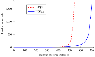
(a) HQS vs. HQS_np – solved instances

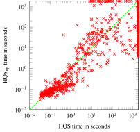
(b) HQS vs. HQS_np – computation time

Figure 4: Impact of Quantifier Localization

Altogether 701 instances out of 991 were solved by HQS_np in the end, whereas HQS could only solve 542. This increases the number of solved instances by more than 29% (for a cactus plot comparing HQS with HQS_np see Figure 4(a)). The largest impact of quantifier localization has been observed on equivalence checking benchmarks for incomplete circuits from [42].

Figure 4(b) shows the computation times of HQS resp. HQS_np for all individual benchmark instances. The figure reveals that quantifier localization, in its current implementation, does not lead to a better result in every case. 186 instances have been solely solved by HQS_np, but the opposite is true for 27 benchmarks. In all of these 27 instances the AIG sizes have grown during local quantifier elimination, and processing larger AIGs resulted in larger run times. Altogether, the size of the AIG after DQBFQuantLocalization has been decreased in 545 cases and increased in 300 cases (in 3 modified instances the number of AIG nodes did not change), although in general it is not unusual that the symbolic elimination of quantifiers must be paid by increasing the sizes of AIGs. Nevertheless, Figure 4(b) shows that in most cases the run times of HQS_np are faster than those of HQS (and, as already mentioned, the number of solved instances is increased by more than 29%).

We also tested our algorithm on the competition benchmarks from QBFEVAL’18 to QBFEVAL’20 [33, 34, 35]. Here the situation is pretty similar. In those competitions 660 different benchmark instances have been used. 141 out of 660 benchmark instances reach our core algorithm and 65 of them could be solved by the original HQS algorithm. In all those 141 instances variables are pushed into the formula, and in 39 instances pushing enabled 3641 local eliminations of variables in total. This made it possible to newly solve 13 benchmark instances and to decrease the runtime for further 10 instances.

6 Conclusions

In this paper, we presented syntax and semantics of non-prenex DQBFs and proved rules to transform prenex DQBFs into non-prenex DQBFs. We could demonstrate that we can achieve significant improvements by extending the DQBF solver HQS based on this theory. Simplifications of DQBFs were due to symbolic quantifier eliminations that were enabled by pushing quantifiers into the formula based on our rules for non-prenex DQBFs.

In the future, we aim at improving the results of quantifier localization, e. g., by introducing estimates on costs and benefits of quantifier localization operations as well as local quantifier elimination and by using limits on the growth of AIG sizes caused by local quantifier elimination.

Appendix A Proof of Theorem 2

See 2

Proof.

We show that $\llbracket\psi\rrbracket_{D}=\llbracket\psi\rrbracket_{T}$ holds by induction on the structure of $\psi$.

(2a):

$v$ is a free variable in $\psi$. Therefore $\mathbb{S}_{\psi}=\{v\mapsto\mathbf{0},v\mapsto\mathbf{1}\}$. Only replacing $v$ by $\mathbf{1}$ turns $\psi$ into a tautology, i. e., $\llbracket\psi\rrbracket_{D}=\{v\mapsto\mathbf{1}\}=\llbracket\psi\rrbracket_{T}$.

(2b):

Like in the first case, $v$ is a free variable in $\psi$. Therefore $\mathbb{S}_{\psi}=\{v\mapsto\mathbf{0},v\mapsto\mathbf{1}\}$. Only replacing $v$ by $\mathbf{0}$ turns $\neg v$ into a tautology, i. e., $\llbracket\psi\rrbracket_{D}=\{v\mapsto\mathbf{0}\}=\llbracket\psi\rrbracket_{T}$.

(2c) $\psi=(\varphi_{1}\land\varphi_{2})$:

$\llbracket\psi\rrbracket_{D}=\bigl{\{}s\in\mathbb{S}_{\psi}\,\big{|}\,\vDash s(\psi)\bigr{\}}=\bigl{\{}s\in\mathbb{S}_{\psi}\,\big{|}\,\vDash s(\varphi_{1})\land s(\varphi_{2})\bigr{\}}$.
The conjunction $s(\varphi_{1})\land s(\varphi_{2})$ is a tautology iff both $s(\varphi_{1})$ and $s(\varphi_{2})$ are tautologies, i. e., $\llbracket\psi\rrbracket_{D}=\bigl{\{}s\in\mathbb{S}_{\psi}\,\big{|}\,{\vDash s(\varphi_{1})}\land{\vDash s(\varphi_{2})}\bigr{\}}$. We can restrict $s$ to the variables that actually occur in the sub-formulas, i. e., $\llbracket\psi\rrbracket_{D}=\bigl{\{}s\in\mathbb{S}_{\psi}\,\big{|}\,{\vDash s_{|V^{\mathrm{free}}_{\varphi_{1}}\mathbin{\dot{\cup}}V^{\exists}_{\varphi_{1}}}(\varphi_{1})}\land{\vDash s_{|V^{\mathrm{free}}_{\varphi_{2}}\mathbin{\dot{\cup}}V^{\exists}_{\varphi_{2}}}(\varphi_{2})}\bigr{\}}$. By using Definition 6 of $\llbracket\cdot\rrbracket_{D}$: $\llbracket\psi\rrbracket_{D}=\bigl{\{}s\in\mathbb{S}_{\psi}\,\big{|}\,s_{|V^{\mathrm{free}}_{\varphi_{1}}\mathbin{\dot{\cup}}V^{\exists}_{\varphi_{1}}}\in\llbracket\varphi_{1}\rrbracket_{D}\land s_{|V^{\mathrm{free}}_{\varphi_{2}}\mathbin{\dot{\cup}}V^{\exists}_{\varphi_{2}}}\in\llbracket\varphi_{2}\rrbracket_{D}\bigr{\}}$. Due to the induction assumption we have $\llbracket\varphi_{1}\rrbracket_{D}=\llbracket\varphi_{1}\rrbracket_{T}$ and $\llbracket\varphi_{2}\rrbracket_{D}=\llbracket\varphi_{2}\rrbracket_{T}$ and thus: $\llbracket\psi\rrbracket_{D}=\bigl{\{}s\in\mathbb{S}_{\psi}\,\big{|}\,s_{|V^{\mathrm{free}}_{\varphi_{1}}\mathbin{\dot{\cup}}V^{\exists}_{\varphi_{1}}}\in\llbracket\varphi_{1}\rrbracket_{T}\land s_{|V^{\mathrm{free}}_{\varphi_{2}}\mathbin{\dot{\cup}}V^{\exists}_{\varphi_{2}}}\in\llbracket\varphi_{2}\rrbracket_{T}\bigr{\}}$. With the definition of $\llbracket\cdot\rrbracket_{T}$ in (2c) we finally obtain:
$\llbracket\psi\rrbracket_{D}=\bigl{\{}s\in\mathbb{S}_{\psi}\,\big{|}\,s\in\llbracket\psi\rrbracket_{T}\bigr{\}}=\llbracket\psi\rrbracket_{T}.$

(2d) $\psi=(\varphi_{1}\lor\varphi_{2})$:

This case is analogous to the previous case, however it needs an additional argument. Here we need the statement ‘The disjunction $s(\varphi_{1})\lor s(\varphi_{2})$ is a tautology iff $s(\varphi_{1})$ or $s(\varphi_{2})$ are tautologies’ which is not true in general. Nevertheless, we can prove it here with the following argument: $s(\varphi_{1})$ only contains variables from $V^{\forall}_{\varphi_{1}}$, and similarly $s(\varphi_{2})$ only variables from $V^{\forall}_{\varphi_{2}}$. According to our assumption from Definition 4 $V^{\forall}_{\varphi_{1}}\cap V^{\forall}_{\varphi_{2}}=\emptyset$ holds. Therefore $s(\varphi_{1})\lor s(\varphi_{2})$ is a tautology iff at least one of its parts is a tautology.

(2e) $\psi=\exists v(D_{v}):\varphi^{-v}$:

$\llbracket\psi\rrbracket_{D}=\bigl{\{}s\in\mathbb{S}_{\psi}\,\big{|}\,\vDash s(\exists v(D_{v}):\varphi^{-v})\bigr{\}}$. The first observation is that $\mathbb{S}_{\psi}=\mathbb{S}_{\varphi^{-v}}$, since $D_{v}\subseteq V\setminus(V^{\exists}_{\varphi}\mathbin{\dot{\cup}}V^{\forall}_{\varphi}\mathbin{\dot{\cup}}\{v\})$, i. e., $D_{v}\cap V^{\forall}_{\varphi}=\emptyset$, and thus Skolem function candidates for $v$ are restricted to constant functions, no matter whether $v$ is a free variable as in $\varphi^{-v}$ or an existential variable without universal variables in its dependency set as in $\psi$. For all other existential variables in $\varphi$, $\varphi^{-v}$ removes $v$ from the dependency sets of all existential variables, but this does not have any effect on the corresponding Skolem function candidates, since $v\notin V^{\forall}_{\varphi}$. Second, for each $s\in\mathbb{S}_{\psi}$ we have $s\bigl{(}\exists v(D_{v}):\varphi\bigr{)}=s\bigl{(}\varphi^{-v}\bigr{)}$. Therefore we get: $\llbracket\psi\rrbracket_{D}=\bigl{\{}s\in\mathbb{S}_{\varphi^{-v}}\,\big{|}\,\vDash s(\varphi^{-v})\bigr{\}}=\llbracket\varphi^{-v}\rrbracket_{D}$. By applying the induction assumption we get $\llbracket\varphi^{-v}\rrbracket_{D}=\llbracket\varphi^{-v}\rrbracket_{T}$ and finally, because of the definition of $\llbracket\cdot\rrbracket_{T}$: $\llbracket\psi\rrbracket_{D}=\llbracket\psi\rrbracket_{T}$.

(2f) $\psi=\forall v:\varphi$:

$\llbracket\psi\rrbracket_{D}=\bigl{\{}t\in\mathbb{S}_{\psi}\,\big{|}\,\vDash t(\forall v:\varphi)\bigr{\}}=\bigl{\{}t\in\mathbb{S}_{\psi}\,\big{|}\,\vDash t(\varphi)\bigr{\}}=\bigl{\{}t\in\mathbb{S}_{\psi}\,\big{|}\,\vDash t(\varphi)[\nicefrac{{0}}{{v}}]\ \land\vDash t(\varphi)[\nicefrac{{1}}{{v}}]\bigr{\}}$. For a function $t\in\mathbb{S}_{\psi}$, we define two functions $s_{0}^{t},s_{1}^{t}\in\mathbb{S}_{\varphi}$ by: $s_{0}^{t}(v)=\mathbf{0}$, $s_{1}^{t}(v)=\mathbf{1}$, $s_{0}^{t}(w)=s_{1}^{t}(w)=t(w)$ if $w\in V^{\exists}_{\varphi}$ with $v\not\in D_{v}$ or $w\in V^{\mathrm{free}}_{\varphi}\setminus\{v\}$, and $s_{0}^{t}(w)=t(w)[\nicefrac{{0}}{{v}}]$, $s_{1}^{t}(w)=t(w)[\nicefrac{{1}}{{v}}]$ for $w\in V^{\exists}_{\varphi}$ with $v\in D_{w}$. Then we have: $t(\varphi)[\nicefrac{{0}}{{v}}]=s_{0}^{t}(\varphi)$ and $t(\varphi)[\nicefrac{{1}}{{v}}]=s_{1}^{t}(\varphi)$. $\llbracket\psi\rrbracket_{D}=\bigl{\{}t\in\mathbb{S}_{\psi}\,\big{|}\,{\vDash s_{0}^{t}(\varphi)}\land{\vDash s_{1}^{t}(\varphi)}\bigr{\}}=\bigl{\{}t\in\mathbb{S}_{\psi}\,\big{|}\,s_{0}^{t}\in\llbracket\varphi\rrbracket_{D}\land s_{1}^{t}\in\llbracket\varphi\rrbracket_{D}\bigr{\}}$. The induction assumption gives us: $\llbracket\varphi\rrbracket_{D}=\llbracket\varphi\rrbracket_{T}$ and therefore: $\llbracket\psi\rrbracket_{D}=\bigl{\{}t\in\mathbb{S}_{\psi}\,\big{|}\,s_{0}^{t}\in\llbracket\varphi\rrbracket_{T}\land s_{1}^{t}\in\llbracket\varphi\rrbracket_{T}\bigr{\}}$. With the equality $t(w)=\mathrm{ITE}\bigl{(}v,t(w)[\nicefrac{{1}}{{v}}],t(w)[\nicefrac{{0}}{{v}}]\bigr{)}=\mathrm{ITE}\bigl{(}v,s_{1}^{t}(w),s_{0}^{t}(w)\bigr{)}$ for $w\in V^{\exists}_{\varphi}=V^{\exists}_{\psi}$ with $v\in D_{w}$ and $t(w)=s_{0}^{t}(w)=s_{1}^{t}(w)$ for the remaining existential or free variables, we obtain:

$$\llbracket\psi\rrbracket_{D} =\bigl{\{}t\in\mathbb{S}_{\psi}\,\big{|}\,\exists s_{0},s_{1}\in\llbracket\varphi\rrbracket_{T}:s_{0}(v)=\mathbf{0}\land s_{1}(v)=\mathbf{1}$$

$$\quad\land\;t(w)=s_{0}(w)=s_{1}(w)\text{ for }w\in V^{\mathrm{free}}_{\psi}=V^{\mathrm{free}}_{\varphi}\setminus\{v\}$$

$$\quad\land\;t(w)=s_{0}(w)=s_{1}(w)\text{ for }w\in V^{\exists}_{\psi}\text{ with }v\notin D_{w}$$

$$\quad\land\;t(w)=\mathrm{ITE}\bigl{(}v,s_{1}(w),s_{0}(w)\bigr{)}\text{ for }w\in V^{\exists}_{\psi}\text{ with }v\in D_{w}\bigr{\}}$$

$$=\llbracket\psi\rrbracket_{T}.$$

∎

Appendix B Proof of Theorem 3

See 3

Proof.

(3a):

Since the left-hand side $\exists y(D_{y}):\varphi$ of rule (3a) is a well-defined DQBF, we have $\varphi=\varphi^{-y}$ according to Definition 4. The rule simply follows from $\llbracket\exists y(D_{y}):\varphi^{-y}\rrbracket=\llbracket\varphi^{-y}\rrbracket$ shown in Theorem 2.

(3b):

We omit the proof here, as it immediately follows from the more general Theorem 6.

(3c):

The statement easily follows from Theorem 2, (2f) considering that $\varphi$ contains only free variables. Let $\psi_{1}\colonequals\forall x:\varphi$ and $\psi_{2}\colonequals\varphi[\nicefrac{{0}}{{x}}]\land\varphi[\nicefrac{{1}}{{x}}]$. We have $\mathbb{S}_{\psi_{1}}=\mathbb{S}_{\psi_{2}}$ and $\llbracket\psi_{1}\rrbracket=\bigl{\{}t\in\mathbb{S}_{\psi_{1}}\,\big{|}\,\exists s_{0},s_{1}\in\llbracket\varphi\rrbracket:s_{0}(x)=\mathbf{0}\land s_{1}(x)=\mathbf{1}\;\land\forall w\in V^{\mathrm{free}}_{\psi_{1}}:t(w)\colonequals s_{0}(w)=s_{1}(w)\bigr{\}}=\llbracket\psi_{2}\rrbracket$.

(3d):

Let $\psi_{1}\colonequals\exists y(D_{y}):\varphi$ and $\psi_{2}\colonequals\varphi[\nicefrac{{0}}{{y}}]\lor\varphi[\nicefrac{{1}}{{y}}]$.

Assume that $\llbracket\psi_{1}\rrbracket\neq\emptyset$ and let $t\in\llbracket\psi_{1}\rrbracket$. $t(y)$ has to be a constant function, i. e., $t(y)=\mathbf{0}$ or $t(y)=\mathbf{1}$. We choose a Skolem function $t^{\prime}$ for $\psi_{2}$ by $t^{\prime}(v)=t(v)$ for all $v\in V^{\mathrm{free}}_{\psi_{2}}$. It is clear that $t^{\prime}$ is a Skolem function candidate for $\psi_{2}$. Assume w. l. o. g. that $t(y)=\mathbf{0}$. Since $t\bigl{(}\exists y(D_{y}):\varphi\bigr{)}=t\bigl{(}\varphi\bigr{)}$ is a tautology, $t^{\prime}\bigl{(}\varphi[\nicefrac{{0}}{{y}}]\bigr{)}=t\bigl{(}\varphi\bigr{)}$ is a tautology, too. Thus, $t^{\prime}\bigl{(}\varphi[\nicefrac{{0}}{{y}}]\lor\varphi[\nicefrac{{1}}{{y}}]\bigr{)}=t^{\prime}\bigl{(}\varphi[\nicefrac{{0}}{{y}}]\bigr{)}\lor t^{\prime}\bigl{(}\varphi[\nicefrac{{1}}{{y}}]\bigr{)}$ is a tautology. This shows that $t^{\prime}\in\llbracket\psi_{2}\rrbracket$ and therefore $\llbracket\psi_{2}\rrbracket\neq\emptyset$.

For the opposite direction assume that $\llbracket\psi_{2}\rrbracket\neq\emptyset$ and let $t^{\prime}\in\llbracket\psi_{2}\rrbracket$. $t^{\prime}\bigl{(}\varphi[\nicefrac{{0}}{{y}}]\lor\varphi[\nicefrac{{1}}{{y}}]\bigr{)}$ is a tautology. Since $\varphi$ contains only free variables, $t^{\prime}\bigl{(}\varphi[\nicefrac{{0}}{{y}}]\bigr{)}$ and $t^{\prime}\bigl{(}\varphi[\nicefrac{{1}}{{y}}]\bigr{)}$ are (equivalent to) constants. At least one of them is $\mathbf{1}$, assume w. l. o. g. $t^{\prime}\bigl{(}\varphi[\nicefrac{{0}}{{y}}]\bigr{)}$. Now we choose $t(v)=t^{\prime}(v)$ for all $v\in V^{\mathrm{free}}_{\psi_{2}}\setminus\{y\}$ and $t(y)=\mathbf{0}$. Since $t\bigl{(}\exists y(D_{y}):\varphi\bigr{)}=t\bigl{(}\varphi\bigr{)}=t^{\prime}\bigl{(}\varphi[\nicefrac{{0}}{{y}}]\bigr{)}=\mathbf{1}$, we have $t\in\llbracket\psi_{1}\rrbracket$ and therefore $\llbracket\psi_{1}\rrbracket\neq\emptyset$.

(3e):

We omit the proof here, since it immediately follows from the more general Theorem 8.

(3f):

We omit the proof here, since it immediately follows from the more general Theorem 9.

(3g):

Let $\psi_{1}\colonequals\forall x:(\varphi_{1}\mathbin{\diamond}\varphi_{2})$ and $\psi_{2}\colonequals\bigl{(}\varphi_{1}\mathbin{\diamond}(\forall x:\varphi_{2})\bigr{)}$ and assume that $x\notin V_{\varphi_{1}}$ and $x\notin D_{y}$ for any $y\in V^{\exists}_{\varphi_{1}}$. Note that we need $x\notin V_{\varphi_{1}}$, since otherwise $\psi_{2}$ would not be well-formed according to Definition 4. From $x\notin D_{y}$ for any $y\in V^{\exists}_{\varphi_{1}}$ we conclude that $\mathbb{S}_{\psi_{1}}=\mathbb{S}_{\psi_{2}}$. Then we have: $\llbracket\psi_{1}\rrbracket=\bigl{\{}s\in\mathbb{S}_{\psi_{1}}\,\big{|}\,\vDash s(\forall x:(\varphi_{1}\mathbin{\diamond}\varphi_{2}))\bigr{\}}=\bigl{\{}s\in\mathbb{S}_{\psi_{1}}\,\big{|}\,\vDash s(\varphi_{1}\mathbin{\diamond}\varphi_{2})\bigr{\}}=\bigl{\{}s\in\mathbb{S}_{\psi_{1}}\,\big{|}\,\vDash s(\varphi_{1}\mathbin{\diamond}(\forall x:\varphi_{2}))\bigr{\}}=\bigl{\{}s\in\mathbb{S}_{\psi_{2}}\,\big{|}\,\vDash s(\varphi_{1}\mathbin{\diamond}(\forall x:\varphi_{2}))\bigr{\}}$, since $\mathbb{S}_{\psi_{1}}=\mathbb{S}_{\psi_{2}}$, and finally $\llbracket\psi_{1}\rrbracket=\llbracket\psi_{2}\rrbracket$.

(3h):

We set $\psi_{1}\colonequals\exists y(D_{y}):(\varphi_{1}\lor\varphi_{2})$ and $\psi_{2}\colonequals\bigl{(}\exists y(D_{y}):\varphi_{1}\bigr{)}\lor\bigl{(}\exists y^{\prime}(D_{y}):\varphi_{2}[\nicefrac{{y^{\prime}}}{{y}}]\bigr{)}$.

$$\llbracket\psi_{1}\rrbracket =\bigl{\{}t\in\mathbb{S}_{\psi_{1}}\,\big{|}\,{\vDash t(\exists y(D_{y}):(\varphi_{1}\lor\varphi_{2}))}\bigr{\}}$$

$$=\bigl{\{}t\in\mathbb{S}_{\psi_{1}}\,\big{|}\,{\vDash t(\varphi_{1}\lor\varphi_{2})}\bigr{\}}$$

$$=\bigl{\{}t\in\mathbb{S}_{\psi_{1}}\,\big{|}\,{\vDash t(\varphi_{1})}\lor{\vDash t(\varphi_{2})}\bigr{\}}$$

The last equality holds, because the variables occurring in $$t(\varphi_{1}) t(\varphi_{2})$$ and are disjoint. On the other hand we have

$$\llbracket\psi_{2}\rrbracket =\bigl{\{}t^{\prime}\in\mathbb{S}_{\psi_{2}}\,\big{|}\,{\vDash t^{\prime}((\exists y(D_{y}):\varphi_{1})\lor(\exists y^{\prime}(D_{y}):\varphi_{2}[\nicefrac{{y^{\prime}}}{{y}}]))}\bigr{\}}$$

$$=\bigl{\{}t^{\prime}\in\mathbb{S}_{\psi_{2}}\,\big{|}\,{\vDash t^{\prime}(\varphi_{1}\lor\varphi_{2}[\nicefrac{{y^{\prime}}}{{y}}])}\bigr{\}}$$

$$=\bigl{\{}t^{\prime}\in\mathbb{S}_{\psi_{2}}\,\big{|}\,{\vDash t^{\prime}(\varphi_{1})}\lor{\vDash t^{\prime}(\varphi_{2}[\nicefrac{{y^{\prime}}}{{y}}])}\bigr{\}}.$$

Again, the last equality holds, because the variables occurring in $t^{\prime}(\varphi_{1})$ and $t^{\prime}\bigl{(}\varphi_{2}[\nicefrac{{y^{\prime}}}{{y}}]\bigr{)}$ are disjoint.

Assume that $\llbracket\psi_{1}\rrbracket\neq\emptyset$ and let $t\in\llbracket\psi_{1}\rrbracket$. Then $t(\varphi_{1})$ or $t(\varphi_{2})$ is a tautology. We choose a Skolem function $t^{\prime}$ for $\psi_{2}$ by $t^{\prime}(v)=t(v)$ for all $v\in V^{\mathrm{free}}_{\psi_{1}}\mathbin{\dot{\cup}}V^{\exists}_{\psi_{1}}$ and $t^{\prime}(y^{\prime})=t(y)$. (Note that $t(y)$ as well as $t^{\prime}(y^{\prime})$ have to be constant functions according to Def. 5.) If $t(\varphi_{1})$ is a tautology, then $t^{\prime}(\varphi_{1})=t(\varphi_{1})$ is a tautology as well, $t^{\prime}\in\llbracket\psi_{2}\rrbracket$ and therefore $\llbracket\psi_{2}\rrbracket\neq\emptyset$. If $t(\varphi_{1})$ is not a tautology, then $t(\varphi_{2})$ has to be a tautology and $t^{\prime}\bigl{(}\varphi_{2}[\nicefrac{{y^{\prime}}}{{y}}]\bigr{)}=t(\varphi_{2})$ is a tautology as well, $t^{\prime}\in\llbracket\psi_{2}\rrbracket$ and therefore $\llbracket\psi_{2}\rrbracket\neq\emptyset$.

For the opposite direction assume $\llbracket\psi_{2}\rrbracket\neq\emptyset$ and let $t^{\prime}\in\llbracket\psi_{2}\rrbracket$. Then $t^{\prime}(\varphi_{1})$ or $t^{\prime}(\varphi_{2}[\nicefrac{{y^{\prime}}}{{y}}])$ is a tautology. If $t^{\prime}(\varphi_{1})$ is a tautology, we choose the Skolem function for $\psi_{1}$ by $t(v)=t^{\prime}(v)$ for all $v\in V^{\mathrm{free}}_{\psi_{1}}\mathbin{\dot{\cup}}V^{\exists}_{\psi_{1}}$. It immediately follows that $t(\varphi_{1})=t^{\prime}(\varphi_{1})$ is a tautology as well, $t\in\llbracket\psi_{1}\rrbracket$ and therefore $\llbracket\psi_{1}\rrbracket\neq\emptyset$. If $t^{\prime}(\varphi_{1})$ is not a tautology, then $t^{\prime}(\varphi_{2}[\nicefrac{{y^{\prime}}}{{y}}])$ has to be a tautology and we choose the Skolem function for $\psi_{1}$ by $t(v)=t^{\prime}(v)$ for all $v\in(V^{\mathrm{free}}_{\psi_{1}}\mathbin{\dot{\cup}}V^{\exists}_{\psi_{1}})\setminus\{y\}$ and $t(y)=t^{\prime}(y^{\prime})$. Then $t(\varphi_{2})=t^{\prime}\bigl{(}\varphi_{2}[\nicefrac{{y^{\prime}}}{{y}}]\bigr{)}$ is also a tautology and again $t\in\llbracket\psi_{1}\rrbracket$ and therefore $\llbracket\psi_{1}\rrbracket\neq\emptyset$.

(3i):

Let $\psi_{1}\colonequals\exists y(D_{y}):(\varphi_{1}\mathbin{\diamond}\varphi_{2})$ and $\psi_{2}\colonequals\varphi_{1}\mathbin{\diamond}\bigl{(}\exists y(D_{y}):\varphi_{2}\bigr{)}$. Note that we need $y\not\in V_{\varphi_{1}}$, since otherwise $\psi_{2}$ would not be well-formed according to Definition 4. The following equalities hold:

$$\llbracket\psi_{1}\rrbracket =\bigl{\{}s\in\mathbb{S}_{\psi_{1}}\,\big{|}\,{\vDash s(\exists y(D_{y}):(\varphi_{1}\mathbin{\diamond}\varphi_{2}))}\bigr{\}}$$

$$=\bigl{\{}s\in\mathbb{S}_{\psi_{1}}\,\big{|}\,{\vDash s(\varphi_{1}\mathbin{\diamond}\varphi_{2})}\bigr{\}}$$

$$=\bigl{\{}s\in\mathbb{S}_{\psi_{1}}\,\big{|}\,\vDash s(\varphi_{1}\mathbin{\diamond}(\exists y(D_{y}):\varphi_{2}))\bigr{\}}$$

$$=\bigl{\{}s\in\mathbb{S}_{\psi_{2}}\,\big{|}\,\vDash s(\varphi_{1}\mathbin{\diamond}(\exists y(D_{y}):\varphi_{2}))\bigr{\}}\text{ since $\mathbb{S}_{\psi_{1}}=\mathbb{S}_{\psi_{2}}$}$$

$$=\llbracket\psi_{2}\rrbracket\,.$$

(3j):

By applying Theorem 2, Equation (2e) multiple times, we get: $\llbracket\exists y_{1}(D_{y_{1}})\exists y_{2}(D_{y_{2}}):\varphi\rrbracket=\llbracket\exists y_{2}(D_{y_{2}}):\varphi\rrbracket=\llbracket\varphi\rrbracket=\llbracket\exists y_{1}(D_{y_{1}}):\varphi\rrbracket=\llbracket\exists y_{2}(D_{y_{2}})\exists y_{1}(D_{y_{1}}):\varphi\rrbracket$.

(3k):

We set $\psi_{1}\colonequals\forall x_{1}\forall x_{2}:\varphi$ and $\psi_{2}\colonequals\forall x_{2}\forall x_{1}:\varphi$. Then we have: $\llbracket\psi_{1}\rrbracket=\llbracket\forall x_{1}\forall x_{2}:\varphi\rrbracket=\bigl{\{}s\in\mathbb{S}_{\psi_{1}}\,\big{|}\,{\vDash s(\forall x_{1}\forall x_{2}:\varphi)}\bigr{\}}=\bigl{\{}s\in\mathbb{S}_{\psi_{1}}\,\big{|}\,{\vDash s(\varphi)}\bigr{\}}=\bigl{\{}s\in\mathbb{S}_{\psi_{2}}\,\big{|}\,{\vDash s(\varphi)}\bigr{\}}$, since $\mathbb{S}_{\psi_{1}}=\mathbb{S}_{\psi_{2}}$, and then $\llbracket\psi_{1}\rrbracket=\bigl{\{}s\in\mathbb{S}_{\psi_{2}}\,\big{|}\,{\vDash s(\forall x_{2}\forall x_{1}:\varphi)}\bigr{\}}=\llbracket\psi_{2}\rrbracket$.

(3l):

We set $\psi_{1}\colonequals\forall x\exists y(D_{y}):\varphi$ and $\psi_{2}\colonequals\exists y(D_{y})\forall x:\varphi$.

First note that $\exists y(D_{y})\forall x:\varphi$ is not well-formed according to Definition 4 if $x\in D_{y}$, because $x$ is universal in $\forall x:\varphi$. With $x\notin D_{y}$ we show that $\llbracket\psi_{1}\rrbracket=\llbracket\psi_{2}\rrbracket$. We have: $\llbracket\psi_{1}\rrbracket=\bigl{\{}s\in\mathbb{S}_{\psi_{1}}\,\big{|}\,{\vDash s(\forall x\exists y(D_{y}):\varphi)}\bigr{\}}=\bigl{\{}s\in\mathbb{S}_{\psi_{1}}\,\big{|}\,{\vDash s(\varphi)}\bigr{\}}$. Because $x\notin D_{y}$, the Skolem function candidates for $y$ in $\psi_{1}$ are restricted to constant functions. The same holds for $y$ in $\psi_{2}$. Therefore $\mathbb{S}_{\psi_{1}}=\mathbb{S}_{\psi_{2}}$ is true. So we can write: $\llbracket\psi_{1}\rrbracket=\bigl{\{}s\in\mathbb{S}_{\psi_{2}}\,\big{|}\,{\vDash s(\varphi)}\bigr{\}}=\bigl{\{}s\in\mathbb{S}_{\psi_{2}}\,\big{|}\,{\vDash s(\exists y(D_{y})\forall x:\varphi)}\bigr{\}}=\llbracket\psi_{2}\rrbracket$.

∎

Appendix C Proof of Theorem 7

See 7

Proof.

We show equisatisfiability by proving that $\llbracket\psi^{\prime}\rrbracket\neq\emptyset$ implies $\llbracket\psi\rrbracket\neq\emptyset$ and vice versa. First assume that there is a Skolem function $s^{\prime}\in\llbracket\psi^{\prime}\rrbracket$ with $\vDash s^{\prime}(\psi^{\prime})$. We define $s\in\mathbb{S}_{\psi}$ by $s(v)\colonequals s^{\prime}(v)$ for all $v\in V^{\exists}_{\psi^{\prime}}\cup V^{\mathrm{free}}_{\psi^{\prime}}\setminus\{y\}$ and $s(y)\colonequals s^{\prime}(\varphi[\nicefrac{{1}}{{y}}])$. Since $\varphi$ contains only variables from $D_{y}\cup V^{\mathrm{free}}_{\psi}\cup\{v\in V^{\exists}_{\psi}\;|\;D_{v}\subseteq D_{y}\}$, $\operatorname{supp}\bigl{(}s(y)\bigr{)}=\operatorname{supp}\bigl{(}s^{\prime}(\varphi[\nicefrac{{1}}{{y}}])\bigr{)}\subseteq D_{y}$, i. e., $s\in\mathbb{S}_{\psi}$. By definition of $s(y)$, $s(\psi)$ is the same as $s^{\prime}(\psi^{\prime\prime})$ where $\psi^{\prime\prime}$ results from $\psi$ by replacing the subformula $\varphi$ by $\varphi[\nicefrac{{\varphi[\nicefrac{{1}}{{y}}]}}{{y}}]$. According to [36], quantifier elimination can be done by composition as well and $\varphi[\nicefrac{{\varphi[\nicefrac{{1}}{{y}}]}}{{y}}]$ is equivalent to $\varphi[\nicefrac{{0}}{{y}}]\lor\varphi[\nicefrac{{1}}{{y}}]$, i. e., $s(\psi)=s^{\prime}(\psi^{\prime})$ and thus $\vDash s(\psi)$.

Now assume $s\in\llbracket\psi\rrbracket$ with $\vDash s(\psi)$. Consider $s^{\prime}$ which results from $s$ by removing $y$ from the domain of $s$. Then $s^{\prime}(\varphi)$ can be regarded as a Boolean function depending on $D_{y}\cup\{y\}$. $s(\varphi)=s^{\prime}(\varphi)[\nicefrac{{s(y)}}{{y}}]$ is a function which (1) does not depend on $y$ and which (2) has the property that for each assignment $\mu$ to the variables from $D_{y}\cup\{y\}$ $\mu\bigl{(}s^{\prime}(\varphi)[\nicefrac{{s(y)}}{{y}}]\bigr{)}=\mu\bigl{(}s^{\prime}(\varphi)\bigr{)}$ or $\mu^{\prime}\bigl{(}s^{\prime}(\varphi)[\nicefrac{{s(y)}}{{y}}]\bigr{)}=\mu^{\prime}\bigl{(}s^{\prime}(\varphi)\bigr{)}$ with $\mu^{\prime}$ resulting from $\mu$ by flipping the assignment to $y$. $s^{\prime}(\varphi)[\nicefrac{{s^{\prime}(\varphi)[\nicefrac{{1}}{{y}}]}}{{y}}]$ which corresponds to the existential quantification of $y$ in $s^{\prime}(\varphi)$ is the largest function fulfilling (1) and (2), i. e., $s(\varphi)\leq s^{\prime}(\varphi)[\nicefrac{{s^{\prime}(\varphi)[\nicefrac{{1}}{{y}}]}}{{y}}]$. We derive $s^{\prime\prime}$ from $s$ by replacing $s(y)$ by $s^{\prime}(\varphi)[\nicefrac{{1}}{{y}}]$ and obtain also $s(\psi)\leq s^{\prime\prime}(\psi)$, since $\psi$ is in NNF, i. e., contains negations only at the inputs, thus $\varphi$ is not in the scope of any negation in $\psi$, but only in the scope of conjunctions and disjunctions which are monotonic functions. Thus $\vDash s(\psi)$ implies $\vDash s^{\prime\prime}(\psi)$. Again, due to the equivalence of $\varphi[\nicefrac{{\varphi[\nicefrac{{1}}{{y}}]}}{{y}}]$ and $\varphi[\nicefrac{{0}}{{y}}]\lor\varphi[\nicefrac{{1}}{{y}}]$, we conclude $s^{\prime\prime}(\psi)=s^{\prime}(\psi^{\prime})$ and thus $\vDash s^{\prime}(\psi^{\prime})$. ∎

Appendix D Proof of Theorem 8

See 8

Proof.

First, we assume that $\llbracket\psi\rrbracket\neq\emptyset$ and let $t\in\llbracket\psi\rrbracket$, i. e., $t(\psi)$ is a tautology. For $\psi^{\prime}$ we construct a Skolem function $t^{\prime}$ by $t^{\prime}(v)\colonequals t(v)[\nicefrac{{x^{\prime}}}{{x}}]$ for all $v\in V^{\exists}_{\varphi_{2}}$, $t^{\prime}(v)\colonequals t(v)$ otherwise. It is easy to see that $t^{\prime}$ is a Skolem function candidate for $\psi^{\prime}$.

Now assume that $t^{\prime}(\psi^{\prime})$ is not a tautoloy, i. e., there is an assignment $\mu^{\prime}\in\mathbf{A}(V^{\forall}_{\psi^{\prime}})$ with $\mu^{\prime}\bigl{(}t^{\prime}(\psi^{\prime})\bigr{)}=0$. Since $\mu^{\prime}\bigl{(}t(\psi)\bigr{)}=1$, we have $\mu^{\prime}\bigl{(}t(\psi_{1})\bigr{)}=1$ and $\mu^{\prime}\bigl{(}t^{\prime}(\psi_{2})\bigr{)}=0$ according to Lemma 1. With $\psi_{2}=\bigl{(}\forall x:\varphi_{1}\bigr{)}\land\bigl{(}\forall x^{\prime}:\varphi_{2}[\nicefrac{{x^{\prime}}}{{x}}]\bigr{)}$ we obtain $\mu^{\prime}\bigl{(}t^{\prime}(\forall x:\varphi_{1})\bigr{)}=\mu^{\prime}\bigl{(}t^{\prime}(\varphi_{1})\bigr{)}=0$ or $\mu^{\prime}\bigl{(}t^{\prime}(\forall x^{\prime}:\varphi_{2}[\nicefrac{{x^{\prime}}}{{x}}])\bigr{)}=\mu^{\prime}\bigl{(}t^{\prime}(\varphi_{2}[\nicefrac{{x^{\prime}}}{{x}}])\bigr{)}=0$. In the first case we have $\mu^{\prime}\bigl{(}t(\varphi_{1})\bigr{)}=\mu^{\prime}\bigl{(}t^{\prime}(\varphi_{1})\bigr{)}=0$ which contradicts $\mu^{\prime}\bigl{(}t(\psi_{1})\bigr{)}=\mu^{\prime}\bigl{(}t(\varphi_{1}\land\varphi_{2})\bigr{)}=\mu^{\prime}\bigl{(}t(\varphi_{1})\bigr{)}\land\mu^{\prime}\bigl{(}t(\varphi_{2})\bigr{)}=1$. In the second case we define $\mu\in\mathbf{A}(V^{\forall}_{\psi})$ by $\mu(v)=\mu^{\prime}(v)$ for all $v\in V^{\forall}_{\psi}\setminus\{x\}$ and $\mu(x)=\mu^{\prime}(x^{\prime})$. In this case we obtain $\mu\bigl{(}t(\varphi_{2})\bigr{)}=\mu^{\prime}\bigl{(}t^{\prime}(\varphi_{2}[\nicefrac{{x^{\prime}}}{{x}}]))\bigr{)}=0$. Thus we obtain $\mu\bigl{(}t(\forall x:(\varphi_{1}\land\varphi_{2}))\bigr{)}=\mu\bigl{(}t(\varphi_{1})\land t(\varphi_{2})\bigr{)}=\mu\bigl{(}t(\varphi_{1})\bigr{)}\land\mu\bigl{(}t(\varphi_{2})\bigr{)}=0$. Since $\psi$ and $\psi^{\prime}$ only differ in the $\psi_{1}$-/$\psi_{2}$-part and the only occurrences of $x$ in $t(\psi)$ are in $t(\psi_{1})$, this leads to $\mu\bigl{(}t(\psi)\bigr{)}=\mu^{\prime}\bigl{(}t^{\prime}(\psi^{\prime})\bigr{)}=0$, which is a contradiction to the fact that $t(\psi)$ is a tautology. Thus, $t^{\prime}(\psi^{\prime})$ has to be a tautology as well and $\llbracket\psi^{\prime}\rrbracket\neq\emptyset$.

For the opposite direction we assume that $\llbracket\psi^{\prime}\rrbracket\neq\emptyset$ and let $t^{\prime}\in\llbracket\psi^{\prime}\rrbracket$. We obtain $\llbracket\psi\rrbracket\neq\emptyset$ with similar arguments: We construct a Skolem function $t$ for $\psi$ as follows: $t(v)=t^{\prime}(v)[\nicefrac{{x}}{{x^{\prime}}}]$ for $v\in V^{\exists}_{\varphi_{2}}$ and $t(v)=t^{\prime}(v)$ otherwise. Assume that $t(\psi)$ is not a tautology, i. e., there is an assignment $\mu\in\mathbf{A}(V^{\forall}_{\psi})$ with $\mu\bigl{(}t(\psi)\bigr{)}=0$ and define $\mu^{\prime}\in\mathbf{A}(V^{\forall}_{\psi^{\prime}})$ by $\mu^{\prime}(v)\colonequals\mu(v)$ for all $v\in V^{\forall}_{\psi}$ as well as $\mu^{\prime}(x^{\prime})\colonequals\mu(x)$. $\mu^{\prime}\bigl{(}t^{\prime}(\psi^{\prime})\bigr{)}=1$ because $t^{\prime}(\psi^{\prime})$ is a tautology. We obtain $\mu^{\prime}\bigl{(}t^{\prime}(\psi_{2})\bigr{)}=1$ and $\mu^{\prime}\bigl{(}t(\psi_{1})\bigr{)}=\mu\bigl{(}t(\psi_{1})\bigr{)}=0$ as above by Lemma 1. From $\mu\bigl{(}t(\psi_{1})\bigr{)}=0$ we conclude $\mu\bigl{(}t(\varphi_{1})\bigr{)}=0$ or $\mu\bigl{(}t(\varphi_{2})\bigr{)}=0$. Since $\mu^{\prime}\bigl{(}t^{\prime}(\varphi_{1})\bigr{)}=\mu\bigl{(}t(\varphi_{1})\bigr{)}$ and $\mu^{\prime}\bigl{(}t^{\prime}(\varphi_{2}[\nicefrac{{x^{\prime}}}{{x}}])\bigr{)}=\mu\bigl{(}t(\varphi_{2})\bigr{)}$, this implies $\mu^{\prime}\bigl{(}t^{\prime}((\forall x:\varphi_{1})\land(\forall x^{\prime}:\varphi_{2}[\nicefrac{{x^{\prime}}}{{x}}]))\bigr{)}=0$ which contradicts $\mu^{\prime}\bigl{(}t^{\prime}(\psi_{2})\bigr{)}=1$ derived above. Thus, $t(\psi)$ is a tautology and $\llbracket\psi\rrbracket\neq\emptyset$. ∎

References

- [1] A. Ge-Ernst, C. Scholl, R. Wimmer, Localizing quantifiers for DQBF, in: C. Barrett, J. Yang (Eds.), Int’l Conf. on Formal Methods in Computer Aided Design (FMCAD), IEEE, 2019, pp. 184–192. doi:10.23919/FMCAD.2019.8894269.
- [2] J. Rintanen, K. Heljanko, I. Niemelä, Planning as satisfiability: parallel plans and algorithms for plan search, Artificial Intelligence 170 (12–13) (2006) 1031–1080. doi:10.1016/j.artint.2006.08.002.
- [3] S. Eggersglüß, R. Drechsler, A highly fault-efficient SAT-based ATPG flow, IEEE Design & Test of Computers 29 (4) (2012) 63–70. doi:10.1109/MDT.2012.2205479.
- [4] A. Czutro, I. Polian, M. D. T. Lewis, P. Engelke, S. M. Reddy, B. Becker, Thread-parallel integrated test pattern generator utilizing satisfiability analysis, Int’l Journal of Parallel Programming 38 (3–4) (2010) 185–202. doi:10.1007/s10766-009-0124-7.
- [5] A. Biere, A. Cimatti, E. M. Clarke, O. Strichman, Y. Zhu, Bounded model checking, Advances in Computers 58 (2003) 117–148. doi:10.1016/S0065-2458(03)58003-2.
- [6] E. M. Clarke, A. Biere, R. Raimi, Y. Zhu, Bounded model checking using satisfiability solving, Formal Methods in System Design 19 (1) (2001) 7–34. doi:10.1023/A:1011276507260.
- [7] F. Ivancic, Z. Yang, M. K. Ganai, A. Gupta, P. Ashar, Efficient SAT-based bounded model checking for software verification, Theoretical Computer Science 404 (3) (2008) 256–274. doi:10.1016/j.tcs.2008.03.013.
- [8] F. Lonsing, A. Biere, DepQBF: A dependency-aware QBF solver, Journal on Satisfiability, Boolean Modelling and Computation 7 (2–3) (2010) 71–76. doi:10.3233/sat190077.
- [9] M. Janota, W. Klieber, J. Marques-Silva, E. M. Clarke, Solving QBF with counterexample guided refinement, in: A. Cimatti, R. Sebastiani (Eds.), Int’l Conf. on Theory and Applications of Satisfiability Testing (SAT), Vol. 7317 of LNCS, Springer, Trento, Italy, 2012, pp. 114–128. doi:10.1007/978-3-642-31612-8_10.
-
[10]
M. Janota, J. Marques-Silva, Solving
QBF by clause selection, in: Q. Yang, M. Wooldridge (Eds.), Int’l Joint
Conf. on Artificial Intelligence (IJCAI), AAAI Press, Buenos Aires,
Argentina, 2015, pp. 325–331.
URL http://ijcai.org/Abstract/15/052 - [11] L. Tentrup, M. N. Rabe, CAQE: A certifying QBF solver, in: Int’l Conf. on Formal Methods in Computer Aided Design (FMCAD), IEEE, Austin, TX, USA, 2015, pp. 136–143. doi:10.1109/FMCAD.2015.7542263.
- [12] G. Peterson, J. Reif, S. Azhar, Lower bounds for multiplayer non-cooperative games of incomplete information, Computers & Mathematics with Applications 41 (7–8) (2001) 957–992. doi:10.1016/S0898-1221(00)00333-3.
- [13] V. Balabanov, H. K. Chiang, J. R. Jiang, Henkin quantifiers and Boolean formulae: A certification perspective of DQBF, Theoretical Computer Science 523 (2014) 86–100. doi:10.1016/j.tcs.2013.12.020.
- [14] R. Bloem, R. Könighofer, M. Seidl, SAT-based synthesis methods for safety specs, in: K. L. McMillan, X. Rival (Eds.), Int’l Conf. on Verification, Model Checking, and Abstract Interpretation (VMCAI), Vol. 8318 of LNCS, Springer, San Diego, CA, USA, 2014, pp. 1–20. doi:10.1007/978-3-642-54013-4_1.
- [15] K. Chatterjee, T. A. Henzinger, J. Otop, A. Pavlogiannis, Distributed synthesis for LTL fragments, in: Int’l Conf. on Formal Methods in Computer Aided Design (FMCAD), IEEE, 2013, pp. 18–25. doi:10.1109/FMCAD.2013.6679386.
- [16] C. Scholl, B. Becker, Checking equivalence for partial implementations, in: ACM/IEEE Design Automation Conference (DAC), ACM Press, Las Vegas, NV, USA, 2001, pp. 238–243. doi:10.1145/378239.378471.
- [17] K. Gitina, S. Reimer, M. Sauer, R. Wimmer, C. Scholl, B. Becker, Equivalence checking of partial designs using dependency quantified Boolean formulae, in: IEEE Int’l Conf. on Computer Design (ICCD), IEEE Computer Society, Asheville, NC, USA, 2013, pp. 396–403. doi:10.1109/ICCD.2013.6657071.
- [18] L. Henkin, Some remarks on infinitely long formulas, in: Infinitistic Methods: Proc. of the 1959 Symp. on Foundations of Mathematics, Pergamon Press, Warsaw, Panstwowe, 1961, pp. 167–183.
- [19] A. Fröhlich, G. Kovásznai, A. Biere, H. Veith, iDQ: Instantiation-based DQBF solving, in: D. L. Berre (Ed.), Int’l Workshop on Pragmatics of SAT (POS), Vol. 27 of EPiC Series, EasyChair, Vienna, Austria, 2014, pp. 103–116. doi:10.29007/1s5k.
- [20] K. Gitina, R. Wimmer, S. Reimer, M. Sauer, C. Scholl, B. Becker, Solving DQBF through quantifier elimination, in: Int’l Conf. on Design, Automation & Test in Europe (DATE), IEEE, Grenoble, France, 2015, pp. 1617–1622. doi:10.7873/DATE.2015.0098.
- [21] R. Wimmer, K. Gitina, J. Nist, C. Scholl, B. Becker, Preprocessing for DQBF, in: M. Heule, S. Weaver (Eds.), Int’l Conf. on Theory and Applications of Satisfiability Testing (SAT), Vol. 9340 of LNCS, Springer, Austin, TX, USA, 2015, pp. 173–190. doi:10.1007/978-3-319-24318-4_13.
- [22] R. Wimmer, A. Karrenbauer, R. Becker, C. Scholl, B. Becker, From DQBF to QBF by dependency elimination, in: Int’l Conf. on Theory and Applications of Satisfiability Testing (SAT), Vol. 10491 of LNCS, Springer, Melbourne, Australia, 2017, pp. 326–343. doi:10.1007/978-3-319-66263-3_21.
- [23] L. Tentrup, M. N. Rabe, Clausal abstraction for DQBF, in: Int’l Conf. on Theory and Applications of Satisfiability Testing (SAT), LNCS, Springer, Lisboa, Portugal, 2019, pp. 388–405. doi:10.1007/978-3-030-24258-9_27.
- [24] K. Korovin, iProver – an instantiation-based theorem prover for first-order logic (system description), in: A. Armando, P. Baumgartner, G. Dowek (Eds.), Int’l Joint Conf. on Automated Reasoning (IJCAR), Vol. 5195 of LNCS, Springer, Sydney, Australia, 2008, pp. 292–298. doi:10.1007/978-3-540-71070-7_24.
- [25] J. Síč, Satisfiability of DQBF using binary decision diagrams, Master’s thesis, Masaryk University, Brno, Czech Republic (2020).
- [26] M. N. Rabe, A resolution-style proof system for DQBF, in: S. Gaspers, T. Walsh (Eds.), Int’l Conf. on Theory and Applications of Satisfiability Testing (SAT), Vol. 10491 of LNCS, Springer, Melbourne, VIC, Australia, 2017, pp. 314–325. doi:10.1007/978-3-319-66263-3_20.
- [27] D. Geist, I. Beer, Efficient model checking by automated ordering of transition relation partitions, in: Int’l Conf. on Computer-Aided Verification (CAV), Vol. 818 of LNCS, Springer, 1994, pp. 299–310. doi:10.1007/3-540-58179-0_63.
- [28] R. Hojati, S. C. Krishnan, R. K. Brayton, Early quantification and partitioned transition relations, in: IEEE Int’l Conf. on Computer Design (ICCD), IEEE Computer Society, 1996, pp. 12–19. doi:10.1109/ICCD.1996.563525.
- [29] G. Cabodi, P. Camurati, L. Lavagno, S. Quer, Disjunctive partitioning and partial iterative squaring: An effective approach for symbolic traversal of large circuits, in: ACM/IEEE Design Automation Conference (DAC), ACM Press, 1997, pp. 728–733. doi:10.1145/266021.266355.
- [30] I. Moon, J. H. Kukula, K. Ravi, F. Somenzi, To split or to conjoin: the question in image computation, in: ACM/IEEE Design Automation Conference (DAC), ACM, 2000, pp. 23–28. doi:10.1145/337292.337305.
- [31] M. Benedetti, Quantifier trees for QBFs, in: F. Bacchus, T. Walsh (Eds.), Int’l Conf. on Theory and Applications of Satisfiability Testing (SAT), Vol. 3569 of LNCS, Springer, St. Andrews, UK, 2005, pp. 378–385. doi:10.1007/11499107_28.
- [32] F. Pigorsch, C. Scholl, Exploiting structure in an AIG based QBF solver, in: Int’l Conf. on Design, Automation & Test in Europe (DATE), IEEE, Nice, France, 2009, pp. 1596–1601. doi:10.1109/DATE.2009.5090919.
-
[33]
L. Pulina, M. Seidl, QBFEval’18
– Competitive evaluation of QBF solvers (2018).
URL http://www.qbflib.org/qbfeval18.php -
[34]
L. Pulina, M. Seidl, A. Shukla,
QBFEval’19 – Competitive
evaluation of QBF solvers (2019).
URL http://www.qbflib.org/qbfeval19.php -
[35]
L. Pulina, M. Seidl, A. Shukla,
QBFEval’20 – Competitive
evaluation of QBF solvers (2020).
URL http://www.qbflib.org/qbfeval20.php - [36] J. R. Jiang, Quantifier elimination via functional composition, in: A. Bouajjani, O. Maler (Eds.), Int’l Conf. on Computer-Aided Verification (CAV), Vol. 5643 of LNCS, Springer, Grenoble, France, 2009, pp. 383–397. doi:10.1007/978-3-642-02658-4_30.
- [37] A. Kuehlmann, V. Paruthi, F. Krohm, M. K. Ganai, Robust Boolean reasoning for equivalence checking and functional property verification, IEEE Transactions on CAD of Integrated Circuits and Systems 21 (12) (2002) 1377–1394. doi:10.1109/TCAD.2002.804386.
- [38] R. Wimmer, C. Scholl, B. Becker, The (D)QBF preprocessor HQSpre – Underlying theory and its implementation, Journal on Satisfiability, Boolean Modeling and Computation 11 (1) (2019) 3–52. doi:10.3233/SAT190115.
- [39] R. Wimmer, S. Reimer, P. Marin, B. Becker, HQSpre – An effective preprocessor for QBF and DQBF, in: A. Legay, T. Margaria (Eds.), Int’l Conf. on Tools and Algorithms for the Construction and Analysis of Systems (TACAS), Vol. 10205 of LNCS, Springer, Uppsala, Sweden, 2017, pp. 373–390. doi:10.1007/978-3-662-54577-5_21.
- [40] K. Wimmer, R. Wimmer, C. Scholl, B. Becker, Skolem functions for DQBF, in: C. Artho, A. Legay, D. Peled (Eds.), Int’l Symposium on Automated Technology for Verification and Analysis (ATVA), Vol. 9938 of LNCS, Chiba, Japan, 2016, pp. 395–411. doi:10.1007/978-3-319-46520-3_25.
- [41] R. Wimmer, K. Gitina, J. Nist, C. Scholl, B. Becker, Preprocessing for DQBF, Reports of SFB/TR 14 AVACS 110, SFB/TR 14 AVACS, online available at http://www.avacs.org (Jul. 2015).
- [42] B. Finkbeiner, L. Tentrup, Fast DQBF refutation, in: C. Sinz, U. Egly (Eds.), Int’l Conf. on Theory and Applications of Satisfiability Testing (SAT), Vol. 8561 of LNCS, Springer, Vienna, Austria, 2014, pp. 243–251. doi:10.1007/978-3-319-09284-3_19.
- [43] V. Balabanov, J.-H. R. Jiang, Reducing satisfiability and reachability to DQBF, talk at the Int’l Workshop on Quantified Boolean Formulas (QBF) (Sep. 2015).