See pages - of titlepage/front.pdf

Copyright © 2018 Massimo Nazaria
  Author’s Address
Massimo Nazaria
Sapienza University of Rome
Department of Computer Science
Via Salaria 113, 00198 Rome, Italy
Email: nazaria@di.uniroma1.it

Abstract

Cyber-Physical Systems (CPSs) have become an intrinsic part of the 21st century world. Systems like Smart Grids, Transportation, and Healthcare help us run our lives and businesses smoothly, successfully and safely. Since malfunctions in these CPSs can have serious, expensive, sometimes fatal consequences, System-Level Formal Verification (SLFV) tools are vital to minimise the likelihood of errors occurring during the development process and beyond. Their applicability is supported by the increasingly widespread use of Model Based Design (MBD) tools. MBD enables the simulation of CPS models in order to check for their correct behaviour from the very initial design phase. The disadvantage is that SLFV for complex CPSs is an extremely time-consuming process, which typically requires several months of simulation. Current SLFV tools are aimed at accelerating the verification process with multiple simulators working simultaneously. To this end, they compute all the scenarios in advance in such a way as to split and simulate them in parallel. Furthermore, they compute optimised simulation campaigns in order to simulate common prefixes of these scenarios only once, thus avoiding redundant simulation. Nevertheless, there are still limitations that prevent a more widespread adoption of SLFV tools. Firstly, current tools cannot optimise simulation campaigns from existing datasets with collected scenarios. Secondly, there are currently no methods to predict the time required to complete the SLFV process. This lack of ability to predict the length of the process makes scheduling verification activities highly problematic. In this thesis, we present how we are able to overcome these limitations with the use of a simulation campaign optimiser and an execution time estimator. The optimiser tool is aimed at speeding up the SLFV process by using a data-intensive algorithm to obtain optimised simulation campaigns from existing datasets, that may contain a large quantity of collected scenarios. The estimator tool is able to accurately predict the execution time to simulate a given simulation campaign by using an effective machine-independent method.

To Silvia

List of Acronyms

CPS

Cyber-Physical System

CCP

Coupon Collector’s Problem

DFS

Depth-First Search

DT

Disturbance Trace

LBT

Labels Branching Tree

LCP

Longest Common Prefix

MBD

Model Based Design

MCDS

Model Checking Driven Simulation

ODE

Ordinary Differential Equations

OP

Omission Probability

PWLF

Piecewise Linear Function

RMSE

Root-Mean-Square Error

SBV

Simulation Based Verification

SLFV

System-Level Formal Verification

WCET

Worst Case Execution Time

Chapter 1 Introduction

1.1 Framework

Over the past few decades, we have experienced many technological breakthroughs which have revolutionised the way we live. Cyber-Physical Systems (CPSs) such as smart grid, automotive, and medical systems contribute to ensuring our lives run smoothly, safely and securely. They have become such an intrinsic part of our 21st century world, that few people nowadays could imagine living without them.

Consequently, we have come to expect CPSs to autonomously cope with all the faulty events originating from the environment they operate in. For example, control software in a car must be able to detect any hardware failure and take immediate mitigating action with a high level of autonomy.

In order to achieve this, software components must ensure that all the relevant faulty events from the external environment are promptly detected, and appropriately dealt with in such a way as to either prevent system failures, or recover from temporary malfunctions in a reasonable amount of time.

Since malfunctions in these CPSs can have far-reaching, potentially dangerous, sometimes fatal consequences, it is extremely important to use the most appropriate verification methods over the development life cycle. For this reason, verification activities are performed in parallel with the development process, from the initial design up to the acceptance testing stages.

This is particularly the case at the earliest design stages, where both the cost and effort required to fix design defects can be minimised. Furthermore, the propagation of undiscovered design defects over subsequent stages results in an exponential increase in the reworking needed to resolve them [18].

In fact, the verification of automobile components must prove that the car works as expected in any operating conditions, including engine speed, road surface and ambient temperatures. To this end, thousands of kilometers of road tests are typically needed to verify newly developed components on real vehicles.

Any bug found at this later verification stage has a huge impact on the project schedule and costs. In order to mitigate this, proper simulation methods are used to carry out verification activities as early as possible.

1.2 Model Based System-Level Formal
Verification

Verification methods and tools have long been established as the greatest contributing factor for any successful software development life cycle. Nowadays, there are a variety of verification tools available for all the specific development stages, including system-level design, unit-level coding, integration, and acceptance testing.

Model Based System-Level Formal Verification (SLFV) tools are extremely valuable to fulfil the need to verify the correctness of CPSs being developed during the earliest stages of the development process. One advantage of this model-based approach is that it brings verification forward in the development life cycle. Thus, developers are able to construct, test, and analyse their designs before any system component is implemented. In this way, if major problems are found, they can be resolved with less impact on the budget or schedule of the project.

The goal of SLFV is to use simulation to build confidence that the system as a whole behaves as expected regardless of disturbances originating from the operational environment. Examples of disturbances include sensor $x$ has a failure, and parameter $y$ has been changed. The fact that there are typically a huge number of disturbance scenarios that can originate from the environment makes SLFV of complex CPSs very time-consuming.

Simulation Based Verification

The most commonly used approach to carrying out SLFV is called Simulation Based Verification (SBV), which consists of simulating both hardware and software components of the CPS at the same time in order to reproduce all the relevant operational scenarios. As an example, Figure 1.1 shows a typical SBV setting.

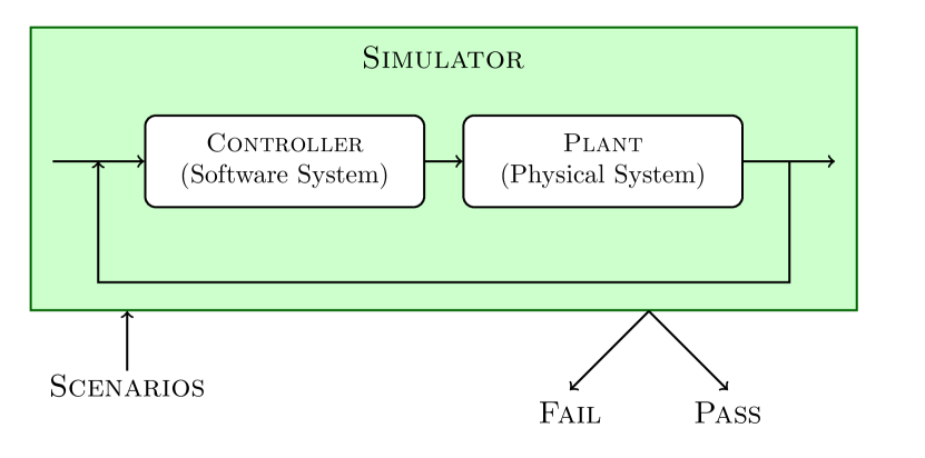
Figure 1.1: Simulation Based Verification

The applicability of SLFV is supported by the increasing use of Model Based Design (MBD) tools to develop CPSs. This is particularly the case within the Automotive, Space, and High-Tech sectors, where tools like Simulink have been established as de facto standards. Such a widespread adoption of MBD tools is mainly due to the fact that they enable SLFV activities at an early stage in the development life cycle.

In this way, when designing a new feature for an existing CPS, modelling and simulation activities can be carried out in order to detect potential design defects that would negatively impact the total development effort and cost. In fact, the re-working that would be required to resolve such defects increases exponentially, if the defects are able to propagate undiscovered over subsequent development stages.

Thus, designers are able to analyse the behaviour of CPSs before actual implementation begins. Needless to say, detecting and fixing errors at the design stage implies significantly less cost and effort compared to later integration and acceptance testing stages.

Another advantage is clearly the potential for shorter time-to-market, which is useful for producers to accelerate getting their product to market so as to maximise the volume of sales after development kickoff.

Simulation Based Verification Process

Figure 1.2 illustrates a high-level diagram of a typical SBV process. In a nutshell, it consists of the following two main phases. First, the Generation Phase where simulation scenarios are generated. Second, the Verification Phase where SBV is carried out.

In the case of failure, design errors are fixed and simulation is repeated until the final output is Pass.

Operational Environment and Safety Properties Specification

SLFV uses formal languages to specify both the environment where the system will operate, and the safety properties it is necessary to satisfy, regardless of any faulty events originating in the specified environment. These formal specification languages include Simulink, and SysML.

As a result of these specifications, SLFV can be performed using an assume-guarantee approach. Namely, an SLFV output of Pass guarantees that the system will behave as expected, assuming that all and only the relevant scenarios are formally specified.

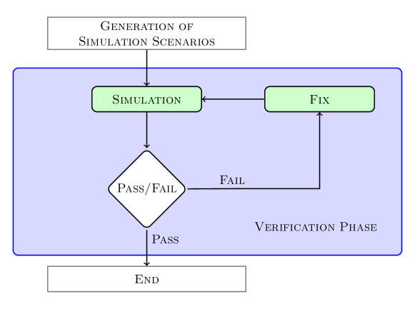
Figure 1.2: Simulation Based System-Level Verification Process

1.3 State of the Art

Notwithstanding the significant advantages of using SLFV, the verification of complex CPSs still remains an extremely time-consuming process. As a matter of fact, SLFV can take up to several months of simulation since it requires a considerable amount of scenarios to be analysed [4].

In order to mitigate this, techniques aimed at speeding up the SLFV process have recently been studied. The two approaches described below use formal methods to specify both the operational environment of the CPS and the safety properties to verify.

1.3.1 System-Level Formal Verification via Parallel
Model Checking Driven Simulation

The approach shown in Figure 1.3 is the so-called Parallel Model Checking Driven Simulation (MCDS) method, which performs SLFV by using a black box approach. This is particularly useful to meet the need to exhaustively analyse the CPS behaviour in all the relevant scenarios that may arise within its operational environment.

This takes place during an initial offline phase where all such scenarios are generated. This upfront generation enables the resulting scenarios to be split into multiple chunks and then simulated in parallel [2][4]. Hence, the MCDS method accelerates the entire SLFV process by involving multiple computing resources which work simultaneously.

Furthermore, the generated scenarios are used to create optimised simulation campaigns with the aim of avoiding redundant simulation. Basically, these campaigns remove this redundancy by simulating duplicate scenarios only once. As a result, SBV is carried out more efficiently by reducing costs and time for simulation activities.

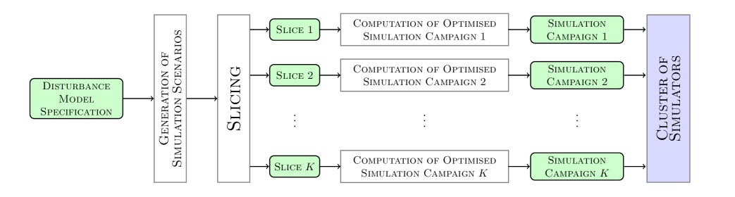
Figure 1.3: SLFV via Parallel Model Checking Driven Simulation

This optimisation is achieved by exploiting the ability of cutting-edge simulation technology (e.g., Simulink) to store the intermediate states of the simulation. These intermediate states are then re-used as the starting point to simulate future scenarios, without the need to start from scratch [2].

Experimental results in [4] show that by using 64 machines with an 8-core processor each, this parallel MCDS approach can complete the SLFV activity in about 27 hours whereas a sequential approach would require more than 200 days.

On top of that, the following benefits can also be exploited from the MCDS method. For example, it can provide online information about the verification coverage, and the Omission Probability (OP) [3][5]. Namely, it can indicate both the number of scenarios simulated so far, and the probability of finding a yet-to-simulate scenario that falsifies a given safety property.

The approach to SLFV that is closest to the MCDS method is presented in [27], where the capability to call external C functions of the model checker CMurphi [12] is exploited in a black box fashion to drive the ESA satellite simulator SIMSAT in order to verify satellite operational procedures. Also in [34], the analogous capability of the model checker SPIN is used to verify actual C code. Both these approaches differ from the MCDS method since they do not consider the optimisation of simulation campaigns.

Statistical and Monte Carlo model checking approaches

Statistical model checking approaches, being basically black box, are also closely related to the MCDS method. For example, [47] addresses SLFV of Simulink models and presents experimental results on the very same Simulink case studies that are used in this thesis. Monte Carlo model checking approaches (see, e.g., [40][43][31]) are also related to this method as well. The main differences between these two latter approaches and the MCDS method are the following: (i) statistical approaches sample the space of admissible simulation scenarios, whereas MCDS addresses exhaustive SBV; (ii) statistical approaches do not address optimisation of the simulation campaign, despite the fact that it makes exhaustive SBV more viable.

Formal verification of Simulink models has been widely investigated, examples are in [42][37][45]. These methods, however, focus on discrete time models (e.g., Simulink/Stateflow restricted to discrete time operators) with small domain variables. Therefore they are well suited to analyse critical subsystems, but cannot handle complex SLVF tasks (i.e., the case studies addressed in this thesis).

This is indeed the motivation for the development of statistical model checking methods as the one in [47] and for exhaustive SBV methods like the MCDS one. For example, in a Model Based Testing setting it has been widely considered the automatic generation of test cases from models (see, e.g., [26]). In SBV settings, instead, automatic generation of simulation scenarios for Simulink has been investigated in [30][35][25][44]. The main differences between these latter approaches and the MCDS method are the following. First, these approaches cannot be used in a black box setting since they generate simulation scenarios from Simulink/Stateflow models, whereas the MCDS method generates scenarios from a formal specification model of disturbances. Second, the above approaches are not exhaustive, whereas the MCDS method is.

Synergies between simulation and formal methods have been widely investigated in digital hardware verification. Examples are in [46][32][39][28] and citations thereof. The main differences between these latter examples and the MCDS method are: (i) they focus on finite state systems, whereas the MCDS method focuses on infinite state systems (namely, hybrid systems); (ii) they are white box (i.e., they require the availability of the CPS model source code) whereas the MCDS method is black box.

The idea of speeding up the SBV process by saving and restoring suitably selected visited states is also present in [28]. Parallel algorithms for explicit state exploration have been widely investigated. Examples are in [41][23][38][24][33]. The main difference between the MCDS method is that these latter ones focus on parallelising the state space exploration engine by devising techniques to minimise locking of the visited state hash table whereas the MCDS method leaves the state space exploration engine (i.e., the simulator) unchanged, and uses an embarrassingly parallel (i.e., map and reduce like [29]) strategy that splits (map step) the set of simulation scenarios into equal size subsets to be simulated on different processors, and stops the SBV process as soon as one of these processors finds an error (reduce step).

The work in [48] also presents an algorithm to estimate the coverage achieved using a SAT based bounded model checking approach. However, since scenarios are not selected uniformly at random, it does not provide any information about the OP, whereas the MCDS method does.

Random model checking, Coverage, and Omission Probability

Random model checking is a formal verification approach closely related to the MCDS method. A random model checker provides, at any time during the verification process, an upperbound to the OP. Upon detection of an error, a random model checker stops and returns a counterexample. Random model checking algorithms have been investigated, e.g., in [31][43][49]. The main differences with respect to the MCDS method are the following: (i) all random model checkers generate simulation scenarios using a sort of Monte-Carlo based random walk. As a result, unlike the MCDS method, none of them is exhaustive (within a finite time horizon); (ii) random model checkers (e.g., see [31]) assume the availability of a lower bound to the probability of selecting an error trace with a random-walk. Being exhaustive, the MCDS method does not make such an assumption.

The coverage yielded by random sampling a set of test cases has been studied by mapping it to the Coupon Collector’s Problem (CCP) (see, e.g., [50]). In the CCP, elements are randomly extracted uniformly and with replacement from a finite set of $n$ test cases (i.e., simulation scenarios in the context of this thesis). Known results (see, e.g., [51]) tell us that the probability distribution of the number of test cases to be extracted in order to collect all $n$ elements has expected value of $\Theta$($n\log{}n$), and a small variance with known bounds. This allows the MCDS method to bound the OP during the SBV process.

Different from CCP based approaches, not only does the MCDS approach bound the OP, but it also grants the completion of the SBV task within just $n$ trials. This is made possible by the fact that simulation scenarios are completely generated upfront.

1.3.2 Probabilistic Temporal Logic Falsification of
Cyber-Physical Systems

Another useful approach to speed up the verification process is the so-called falsification method [15]. Different from the approaches related to, and including, the MCDS method illustrated above, it uses techniques that are aimed at quickly identifying scenarios that falsify the given properties. In other words, these techniques search for operational scenarios where a given requirement specification is not met, hence the evaluation of the corresponding logical property is false. In this way, only a limited number of scenarios are considered, thus less simulation is carried out.

In conclusion, both the aforementioned MCDS and the falsification methods use monitors to discover potential simulation scenarios where the CPS being verified violates a given specification (see, e.g., [36]). These monitors are typically developed manually in the language of the simulator such as the Simulink and Matlab languages. This is an error prone activity that can invalidate the entire verification process, because bugs in these monitors that are due to hand coding mistakes can lead to two significant errors. Firstly, they can result in false positives, i.e., simulation results of Pass which wrongly indicate that the system was able to work as expected under all the given operational scenarios. Secondly, they can result in false negatives, i.e., simulation results of Fail which wrongly points to a scenario were a given requirement was violated.

For this reason, ways to generate monitors directly from formal specifications have recently been presented [16][17][20][21][22]. Clearly, these automatically generated monitors are free of those bugs that are frequently introduced by hand coding.

1.4 Motivations

Despite the fact that SBV tools currently represent the main workhorse for SLFV, they are unlikely to become more widely adopted, unless two limiting factors are overcome.

First of all, the SLFV tool presented in [2] cannot optimise existing datasets, since they may contain a huge number of collected scenarios. In fact, no methods to obtain optimised simulation campaigns from such datasets have yet been studied in spite of the clear need to reduce the time for simulation activities while increasing the quality of these campaigns by removing redundant scenarios.

The second limitation that prevents wider use of current SLFV methods is the lack of prior knowledge of the time needed to complete simulations. The uncertainty surrounding the duration, makes scheduling SLFV activities problematic. For example, underestimating the time needed for simulation activities could result in missed deadlines and costly project delays. Moreover, an overestimated time could result in meeting deadlines long beforehand, which means some resources allocated to the verification task would remain unused.

1.5 Thesis Focus and Contributions to
System-Level Formal Verification

In this thesis, our main focus is on control systems modelled in Simulink, which is a widely used tool in the area of control engineering.

In order to overcome the aforementioned limitations in optimising existing datasets and estimating the time needed for SLFV tasks, we devised and implemented the two following tools: (i) a simulation campaign optimiser, and (ii) an execution time estimator for simulation campaigns.

1.5.1 Simulation Campaign Optimiser

The optimiser tool is aimed at speeding up the SLFV process by avoiding redundant simulation. To this end, we devised and implemented a data-intensive algorithm to obtain optimised simulation campaigns from existing datasets, that may contain a large quantity of collected scenarios. These resulting campaigns are made up of sequences of simulator commands that simulate common prefixes in the given dataset of scenarios only once. These commands include save a simulation state, restore a previously saved simulation state, inject a disturbance on the model, and advance the simulation of a given time length.

Results show that an optimised simulation campaign is at least 3 times faster with respect to the non-optimised one [2]. Furthermore, the presented tool can optimise 4 TB of scenarios in 12 hours using just one core with 50 GB of RAM.

1.5.2 Execution Time Estimator for Simulation
Campaigns

The estimator tool is able to perform an accurate execution time estimate using a partially machine-independent method. In particular, it analyses the numerical integration steps decided by the solver during the simulation. From this preliminary analysis, it first chooses a small set of simulator commands to simulate, and then it collects execution time samples in order to train a prediction function.

Results show that this tool can predict the execution time to simulate a given simulation campaign with an error below 10%.

1.5.3 Publications

The following papers on our two main contributions presented in this thesis are currently being finalised for submission in collaboration with Vadim Alimguzhin, Toni Mancini, Federico Mari, Igor Melatti, and Enrico Tronci.

1. A Data-Intensive Optimiser Tool for Huge Datasets of Simulation Scenarios. To be submitted to Automated Software Engineering.

2. Estimating the Execution Time for Simulation Campaigns with Applications to Simulink. To be submitted to Transactions on Modeling and Computer Simulation.

1.6 Outline

Chapter 2

illustrates background notions and definitions that are used within the thesis.

Chapter 3

presents our optimiser tool. In particular, it first shows the overall method we devised, then it gives details of the algorithm we implemented, finally it presents experimental results regarding the efficiency, scalability, and effectiveness of the method.

Chapter 4

introduces our estimator tool. It gives a detailed description of the method we devised, then it explains how we validated it, finally it presents the experimental results of estimation accuracy.

Chapter 5

draws conclusions and outlines future work.

Chapter 2 Background

2.1 Notation

In this thesis, we use $[n]$ to represent the initial segment $\{1,2,\ldots,n\}$ of natural numbers. Often, we use $\mathbb{N}^{+}$ and $\mathbb{R}^{+}$ to denote the set of natural numbers and positive real numbers respectively. Sometimes, the list concatenation operator is denoted by $\cup$ when we deal with sequences instead of sets.

2.2 Definitions

Disturbance

Definition 2.2.1 (Disturbance).

A disturbance is a number $d\in\mathbb{N}^{+}\cup\{0\}$. A disturbance identifies an exogenous event (e.g. a fault) that we inject into the model being simulated. As an exception, when a disturbance $d$ is zero, we inject nothing on the model, thus a zero indicates what we call the non-disturbance event.

Simulation Interval

Definition 2.2.2 (Simulation Interval).

A simulation interval $\tau$ indicates a fixed amount of simulation seconds. Note that the amount of simulation seconds is usually different from the elapsed time the simulator takes to actually simulate them. In fact, the elapsed time needed to simulate a given simulation interval $\tau$ may be higher or lower than $\tau$, depending on the complexity of the simulation model.

Simulation Scenario

Definition 2.2.3 (Simulation Scenario).

A simulation scenario (or simply scenario) is a finite sequence of disturbances $\delta=(d_{1},d_{2},\ldots,d_{H})$ with length $|\delta|=H$. These disturbances in $\delta$ are associated to $H$ consecutive simulation intervals that have fixed-length $\tau$. In particular, we inject the model with each disturbance $d_{i}\in\delta$ at the beginning of the $i$-th simulation interval. Hence, we simulate $\tau\cdot H$ simulation seconds starting from the initial simulator state, while injecting the model with disturbances at the beginning of each simulation interval.

Simulation Horizon

Definition 2.2.4 (Simulation Horizon).

The simulation horizon (or simply horizon) is the length $H$ of a simulation scenario $\delta=(d_{1},d_{2},\ldots,d_{H})$.

Dataset of Scenarios

Definition 2.2.5 (Dataset of Scenarios).

A dataset of scenarios is a sequence $\Delta=(\delta_{1},\delta_{2},\ldots,\delta_{N})$ that contains a number $|\Delta|=N$ of simulation scenarios. In particular, scenarios in $\Delta$ have horizon $H$. Furthermore, we denote each scenario $\delta_{i}\in\Delta$ by the sequence $\delta_{i}=(d^{i}_{1},d^{i}_{2},\ldots,d^{i}_{H})$.

Simulation Campaign

Definition 2.2.6 (Simulation Campaign).

Given a dataset of scenarios $\Delta$, a simulation campaign is a sequence of simulator commands that we use to simulate the input scenarios in $\Delta$. In particular, we use the five basic commands described in Table 2.1.

Simulator Commands

Table 2.1 shows the five basic simulator commands and their behaviour.

Command	Behaviour
inject($d$)	injects the simulation model with the given disturbance $d\in\mathbb{N}^{+}$
run($t$)	simulates the model for $\tau\cdot t$ simulation seconds, with $t\in[H]$
store($x$)	stores the current state of the simulator on a file named $x$
load($x$)	loads the previously stored state file $x$ into the simulator
free($x$)	removes the previously stored state file $x$

Table 2.1: Simulator Commands

Chapter 3 Optimisation of Huge Datasets of Simulation Scenarios

3.1 Introduction

3.1.1 Framework

The goal of Model Based System-Level Formal Verification (SLFV) for Cyber-Physical Systems (CPSs) is to prove that the system as a whole will behave as expected, regardless of faulty events originating from the environment it operates in. The most widely used approach to SLFV for complex CPSs is called Simulation Based Verification (SBV), and it is supported by the increasing use of Model Based Design (MBD) tools to develop CPSs.

Basically, SBV consists of simulating both hardware and software components at the same time, in order to analyse all the relevant scenarios that the CPS being verified must be able to safely cope with. Due to the risks associated with errors in CPSs, it is extremely important that SBV performs an exhaustive analysis of all the relevant event sequences (i.e., scenarios) that might lead to system failure.

SLFV uses formal languages to specify both the environment where the system will operate, and the safety properties it is necessary to satisfy. As a result of these specifications, SLFV can be performed using an assume-guarantee approach. Namely, a successful SBV process can guarantee that the CPS will behave as expected, assuming that all and only the relevant scenarios are formally specified.

Clearly, the earlier potential errors are identified, the lower the potential costs and effort that are needed to fix them. The fact that MBD tools enable SBV activities to be carried out in the early stages of development life cycle is one of the main reasons for their widespread adoption.

Despite this significant advantage, SBV is still an extremely time-consuming activity. Simulation of complex CPSs can even take as much as several months, since it requires the analysis of a considerable amount of operational scenarios [4].

Techniques aimed at speeding up SBV have recently been explored [2][3][4][5]. They basically exploit cutting-edge simulation technology (e.g., Simulink) that allows for the storage of intermediate states of the simulation. The aim is to reuse the intermediate states as the basis for simulating other future scenarios, instead of having to start again from the initial simulator state [2].

This is achieved by performing an upfront computation of optimised simulation campaigns. In particular, these are made of sequences of simulator instructions that are aimed at simulating common prefixes between scenarios only once, thus removing redundant simulation.

Simulator instructions include save a simulation state, restore a saved simulation state, inject a disturbance on the model, and advance the simulation of a given time length.

3.1.2 Motivations

Unfortunately, these optimised simulation campaigns cannot currently be obtained from existing datasets with a huge number of collected scenarios. The reason for this limitation is that it is computationally expensive to identify common prefixes in large datasets of scenarios.

Consequently, scenarios used in [2] are intentionally generated in a format that makes it easy to spot common prefixes in the resulting dataset. They use a model checker to automatically generate labelled lexicographically-ordered sequences of disturbances, starting from a formal specification model that defines all such sequences.

3.1.3 Contributions

In the following, we show how we overcome this limitation in optimising existing datasets with collected scenarios. Namely, we present a data-intensive optimiser tool to compute optimised simulation campaigns from these datasets.

This tool can efficiently perform the optimisation of a large quantity of scenarios that are unable to fit entirely into the main memory. We accomplish this with a data-intensive algorithm that we describe in detail in this chapter.

In particular, such an algorithm involves a sequence of four distinct steps, that we call initial sorting, load labelling, store labelling, and final optimisation. We designed it in such a way as to minimise both disk I/O latency and the amount of intermediate output data generated at each step, similarly to that offered by current big data computing frameworks such as Apache Hadoop and Apache Spark.

3.2 Problem Formulation

Starting from a dataset $\Delta$ with input scenarios, we generate the corresponding optimised simulation campaign.

The aim is to exploit the capability of modern simulators to store and restore intermediate states thus removing the need to explore common paths of scenarios multiple times.

To be precise, let be given a scenario $\delta=(d_{1},\ldots,d_{H})\in\Delta$. The simulator runs under the input $\delta$ starting from its initial state. Thus, any disturbance $d_{i}\in\delta$, with $1\leq i\leq H$, unequivocally identifies the state reached by the simulator immediately after the $i$-th simulation interval of $\delta$.

Since many scenarios in $\Delta$ share common prefixes of simulation intervals, many simulations which explore the same states multiple times can be considered redundant.

For example, let be given two scenarios $\delta=(\hat{d}_{1},\ldots,\hat{d}_{p},d_{p+1},\ldots,d_{H})$, and $\delta^{\prime}=(\hat{d}_{1},\ldots,\hat{d}_{p},d^{\prime}_{p+1},\ldots,d^{\prime}_{H})$. They share the common prefix $(\hat{d}_{1},\ldots,\hat{d}_{p})$. This prefix would normally be simulated twice for both $\delta$ and $\delta^{\prime}$. This redundancy applies to all the scenarios that share common prefixes in $\Delta$. In the following we show how we avoid the simulation of common prefixes multiple times by exploiting the load/store capabilities of modern simulators.

To simulate the first scenario $\delta$, we: (i) run the simulator with the input being the prefix $(\hat{d}_{1},\ldots,\hat{d}_{p})$; (ii) store the simulator state reached so far with a label $\ell$; (iii) continue the simulation of $\delta$ with the input being the remaining disturbances $(d_{p+1},\ldots,d_{H})$.

To simulate the second scenario $\delta^{\prime}$, we: (i) load back the previously stored state $\ell$ thus avoiding the simulation of the shared prefix $(\hat{d}_{1},\ldots,\hat{d}_{p})$; (ii) continue the simulation of $\delta^{\prime}$ with the input being the remaining disturbances $(d^{\prime}_{p+1},\ldots,d^{\prime}_{H})$.

The difficulty in achieving this, arises from the fact that input scenarios in $\Delta$ are in a format that makes the identification of such prefixes computationally expensive. In particular, input scenarios in $\Delta$ are not lexicographically ordered and do not contain labels to identify common prefixes, differently from the format used in [2]. Furthermore, $\Delta$ may contain as many as millions of scenarios that cannot be entirely accommodated into the available RAM.

3.3 Methodology

3.3.1 Overall Method

In the first step, we uniquely sort the input dataset $\Delta$. The output is a dataset $\mathcal{D}$ that contains a number $|\mathcal{D}|=N$ of distinct lexicographically ordered scenarios. The resulting dataset helps us identify common prefixes during the following step.

In the second step, we compute a file that contains a sequence $\mathcal{L}=(\mathcal{L}_{1},\mathcal{L}_{2},\ldots,\mathcal{L}_{N})$ with $N$ load labels. In particular, every label $\mathcal{L}_{i}$ corresponds to the label of the simulator state that we load at the beginning of the $i$-th scenario in the resulting simulation campaign. More precisely, $\mathcal{L}_{i}$ identifies the simulator state that was previously stored immediately after the simulation of the longest shared prefix of disturbances between the scenario $\delta_{i}\in\mathcal{D}$ and the very first scenario $\delta_{j}\in\mathcal{D}$, with $j<i$, where such a prefix appeared.

In the third step, we uniquely sort the sequence $\mathcal{L}$. The output is a file with a sequence $\mathcal{S}$ of store labels. This resulting sequence helps us spot simulation states to store during the final computation of the simulation campaign in the next step.

Finally, we use the input files $\mathcal{D}$, $\mathcal{L}$, and $\mathcal{S}$ obtained so far in order to compute the final optimised simulation campaign. Basically, we compute a file that contains a sequence $\mathcal{C}$ of simulator commands that avoid the redundant simulation of common paths of scenarios in $\mathcal{D}$ multiple times.

3.3.2 Steps of the Algorithm

Step 1. Initial Sorting

In the first step, we compute a dataset $\mathcal{D}$ of unique lexicographically ordered disturbance sequences, starting from the input dataset $\Delta$, which contains a multiset of unordered disturbance sequences with fixed length $H$.

Since input scenarios in $\Delta$ do not fit entirely into the main memory, an external sorting based approach [14][13] is used to order them. Specifically, we first split these scenarios into smaller chunks and sort them into the main memory. Then, we iteratively merge two sorted chunks at a time, until the last two chunks are merged into the resulting dataset $\mathcal{D}$.

To this end, we allocate two buffers of scenarios in RAM in order to minimise the disk I/O latency. These buffers also help to improve the performance of the other steps where no sorting is involved, namely Step 2 and Step 4 described below.

Step 2. Load Labelling

In this step, we make use of the following labelling strategy in order to compute what we call the sequence of load labels $\mathcal{L}=(\mathcal{L}_{1},\mathcal{L}_{2},\ldots,\mathcal{L}_{N})$ from the dataset $\mathcal{D}=(\mathcal{\delta}_{1},\mathcal{\delta}_{2},\ldots,\mathcal{\delta}_{N})$ which we computed at Step 1.

Each label $\mathcal{L}_{i}$, with $i\in[N]$, is associated to the Longest Common Prefix (LCP) of disturbances between the $i$-th scenario $\delta_{i}$ and all the previous scenarios in $\mathcal{D}$.

Since scenarios in $\mathcal{D}$ are lexicographically ordered, we can easily identify this LCP just by comparing the $i$-th disturbance sequence $\delta_{i}=(d_{1}^{i},\ldots,d_{H}^{i})$ with the previous one $\delta_{i-1}=(d_{1}^{i-1},\ldots,d_{H}^{i-1})$, with $i>1$.

As a result, we obtain the size $p(i)$ of this LCP that we define as

$$p(i):=|\{p\in[H]:\bigwedge\limits_{j=1}^{p}d^{i}_{j}=d^{i-1}_{j}\}|.$$

$p(i)$ represents the index of the rightmost disturbance of the LCP between $\delta_{i}$ and $\delta_{i-1}$. Note that $p(i)=0$ if no common prefix exists, and also that $p(i)$ is always less than $H$, since $\mathcal{D}$ contains no duplicate scenarios.

In order to compute each label $\mathcal{L}_{i}$, we first assign a label $\ell^{i}_{j}$, with $j\in[H]$ to each disturbance $d^{i}_{j}\in\delta_{i}$ in the following way:

$$\ell^{i}_{j}:=\left\{\begin{array}[]{lr}\ell^{i-1}_{j}&\text{if }j\leq p(i)\\ (i-1)\cdot H+j&\text{if }j>p(i)\\ \end{array}\right.$$

Namely, the prefix of disturbances $(d^{i}_{1},d^{i}_{2},\ldots,d^{i}_{p(i)})$ in $\delta_{i}$ share the same labels as the shared prefix $(d^{i-1}_{1},d^{i-1}_{2},\ldots,d^{i-1}_{p(i)})$ in the previous scenario $\delta_{i-1}$. Instead, the remaining disturbances $d^{i}_{j}$ in $\delta_{i}$, with $j\in\{p(i)+1,\ldots,H\}$, are strictly identified by $(i-1)\cdot H+j$.

Finally, each label $\mathcal{L}_{i}$ corresponds to the exact label associated to the rightmost disturbance $d^{i}_{p(i)}\in\delta_{i}$ of the LCP, hence:

$$\mathcal{L}_{i}:=\left\{\begin{array}[]{lr}\ell^{i}_{p(i)}&\text{if }p(i)>0\\ 0&\text{if }p(i)=0\end{array}\right.$$

Note that every label $\mathcal{L}_{i}\in\mathcal{L}$, with $\mathcal{L}_{i}\neq 0$, identifies the simulator state reached immediately after the $(p(i)\text{ }\%\text{ }H)$-th simulation interval of the $\lceil p(i)\text{ }/\text{ }H\rceil$-th scenario $\delta_{\lceil p(i)\text{ }/\text{ }H\rceil}\in\mathcal{D}$. Also note that in order to compute each label $\mathcal{L}_{i}$ there is no need to entirely load $\mathcal{D}$ into the main memory. In fact, all we need is to compare the $i$-th scenario with the previous one.

Step 3. Store Labelling

In this step, we compute a unique lexicographically ordered sequence $\mathcal{S}$ that contains what we call the store labels, starting from the sequence $\mathcal{L}$ computed at Step 2. Sorting is performed using the same strategy we used at Step 1 to obtain $\mathcal{D}$.

The resulting sequence $\mathcal{S}$ contains the same labels in $\mathcal{L}$, but each label in $\mathcal{S}$ appears only once.

We use this sequence of store labels $\mathcal{S}$ during the computation of the final simulation campaign. In particular, $\mathcal{S}$ helps us to spot all those simulator states to store. Labels of store instructions in the resulting campaign appear in the same order as they appear in $\mathcal{S}$.

Note that the first label in $\mathcal{S}$ is always $0$. This is because there is at least the first scenario in $\mathcal{D}$ which shares no common prefixes with previous scenarios, thus $\mathcal{L}_{1}=0$. Also note that since the label $0$ represents the initial simulator state, there is no need to store it. In fact, we assume that this initial state already exists before the simulation begins.

Step 4. Final Optimisation

In this final step, we use the files $\mathcal{D}$, $\mathcal{L}$, and $\mathcal{S}$ obtained at the previous steps in order to compute the optimised simulation campaign.

To this end, we build a sequence $\mathcal{C}=\mathcal{C}_{1}\cup\text{ }\mathcal{C}_{2}\cup\ldots\cup\mathcal{C}_{N}$, where each subsequence $\mathcal{C}_{i}$, with $i\in[N]$, contains simulator commands for the corresponding scenario $\delta_{i}\in\mathcal{D}$. Note that $\cup$ here denotes the list concatenation operator, as defined in Chapter 2.

We use the sequences of labels $\mathcal{S}$ and $\mathcal{L}$ to add commands store and load respectively in the resulting campaign, and are thus able to re-use common simulation states between scenarios.

In addition, we add some commands free in order to remove previously stored simulator states that are no longer needed.

Algorithm 1 describes the approach we use to perform this final step. We compute each subsequence $\mathcal{C}_{i}$ of simulator commands in the following way.

First, we add the commands free (lines from 8 to 11) in order to remove stored simulator states that are no longer needed.

Second, we add the command load (line 14) in order to restore the previously stored simulator state named $\mathcal{L}_{i}$. Note that if $\mathcal{L}_{i}=0$, then the initial simulator state is loaded and the $i$-th scenario $\delta_{i}\in\mathcal{D}$ is completely simulated from the beginning.

Finally, we compute the commands inject, run, and store (lines from 17 to 24). To this end, we first build a sequence of $k$ indexes $(\mathcal{I}_{1},\mathcal{I}_{2},\ldots,\mathcal{I}_{k})$ that has the following properties:

• $\mathcal{I}_{1}$ is the index $p(i)$ of the first time interval in $\delta_{i}$ to simulate;

• $\mathcal{I}_{k}$ is always $H+1$ and we use it to add the last command run (line 21), at the last iteration of the for-loop (line 17);

• All the other indexes $\mathcal{I}_{j}$, with $1<j<k$, correspond to one of these two types of simulation intervals. The first are those intervals where we inject a disturbance $d^{i}_{\mathcal{I}_{j}}$ (line 16), and the second are those ones where we add a command store (line 23) immediately after the simulator state reached by the previous command run (line 21).

Note that there is no need to entirely load $\mathcal{D}$, $\mathcal{L}$, and $\mathcal{S}$ into the main memory. In fact, in order to compute the $i$-th sequence $\mathcal{C}_{i}$ of simulator commands, all we need is the sequence $(d^{i}_{p(i)+1},d^{i}_{p(i)+2},\ldots,d^{i}_{H})\subseteq\delta_{i}$ (line 6), the label $\mathcal{L}_{i}$ (lines 5 and 14), and the first $H-p(i)$ of the remaining labels in $\mathcal{S}$ (lines 16 and 23).

Input: Lex-ordered Dataset $\mathcal{D}=(\delta_{1},\delta_{2},\ldots,\delta_{N})$.

Input: Sequence of Load Labels $\mathcal{L}=(\mathcal{L}_{1},\mathcal{L}_{2},\ldots,\mathcal{L}_{N})$.

Input: Lex-ordered Sequence of Store Labels $\mathcal{S}$.

Output: Sequence of Simulator Commands $\mathcal{C}$.

1

2$\mathcal{C}\leftarrow\varnothing$;

3 $\mathcal{F}\leftarrow(\mathcal{F}_{0},\mathcal{F}_{2},\ldots,\mathcal{F}_{H-1})$ such that $\mathcal{F}_{i}=0$, with $i\in\{0,1,\ldots,H-1\}$;

4

5for each $i\leftarrow 1,2,\ldots,N$ do

6       $\mathcal{C}_{i}\leftarrow\varnothing$;

7       $p(i)\leftarrow\mathcal{L}_{i}\text{ }\%\text{ }H$;

8       $(d^{i}_{p(i)+1},d^{i}_{p(i)+2},\ldots,d^{i}_{H})\subseteq\delta_{i}\in\mathcal{D}$;

9       $\ell^{i}_{j}\leftarrow(i-1)\cdot H+j$, with $j\in\{p(i)+1,p(i)+2,\ldots,H\}$;

10      

11      for each $j\leftarrow p(i)+1,p(i)+2\ldots,H-1$ do

12             if $\mathcal{F}_{j}>0$ then

13                   $\mathcal{C}_{i}\leftarrow\mathcal{C}_{i}\cup\{free(\mathcal{F}_{j})\}$;

14                   $\mathcal{F}_{j}\leftarrow 0$;

15                  

16             end if

17            

18       end for

19      

20      $\mathcal{C}_{i}\leftarrow\mathcal{C}_{i}\cup\{load(\mathcal{L}_{i})\}$;

21       $\mathcal{F}_{p(i)}\leftarrow\mathcal{L}_{i}$;

22      

23      $\mathcal{I}\leftarrow(\mathcal{I}_{1},\mathcal{I}_{2},\ldots,\mathcal{I}_{k})$ such that $\mathcal{I}_{1}=p(i)+1$, $\mathcal{I}_{k}=H+1$, and $(d^{i}_{\mathcal{I}_{j}}\neq 0\text{ }\vee\text{ }\ell^{i}_{\mathcal{I}_{j}-1}\in\mathcal{S})$, with $\mathcal{I}_{1}<\mathcal{I}_{j}<\mathcal{I}_{k}$;

24      

25      for each $j\leftarrow 1,2,\ldots,k-1$ do

26             if $d^{i}_{\mathcal{I}_{j}}\neq 0$ then

27                   $\mathcal{C}_{i}\leftarrow\mathcal{C}_{i}\cup\{inject(d^{i}_{\mathcal{I}_{j}})\}$;

28                  

29             end if

30            $\mathcal{C}_{i}\leftarrow\mathcal{C}_{i}\cup\{run(\mathcal{I}_{j+1}-\mathcal{I}_{j})\}$;

31             if $\ell^{i}_{\mathcal{I}_{j+1}-1}\in\mathcal{S}$ then

32                   $\mathcal{C}_{i}\leftarrow\mathcal{C}_{i}\cup\{store(\ell^{i}_{\mathcal{I}_{j+1}-1})\}$;

33                   $\mathcal{S}\leftarrow\mathcal{S}\setminus\ell^{i}_{\mathcal{I}_{j+1}-1}$;

34                  

35             end if

36            

37       end for

38      $\mathcal{C}\leftarrow\mathcal{C}\cup\mathcal{C}_{i}$;

39      

40 end for

41

Algorithm 1 Computation of the Optimised Simulation Campaign

3.3.3 Correctness of the Algorithm

Prefix-Tree of Scenarios

Let’s define $T_{\mathcal{D}}=(V,E)$ as the prefix-tree of scenarios in $\mathcal{D}$. In particular, $T_{\mathcal{D}}$ is a tree with height $H$, and $V=\mathcal{S}$ $\cup$ $\{0\}$. Namely, the set of vertexes $V$ of $T_{\mathcal{D}}$ contains the simulator state labels in $\mathcal{S}$ including the initial state label $0$, which is the root of $T_{\mathcal{D}}$.

The set of edges $E$ of $T_{\mathcal{D}}$ is composed in such a way that every path $P^{i}=(0,e^{i}_{1},v^{i}_{1},e^{i}_{2},v^{i}_{2},\ldots,e^{i}_{H},v^{i}_{H})$ in $T_{\mathcal{D}}$ corresponds to the exact scenario $\delta_{i}$ in $\mathcal{D}$ and vice versa, with $i\in[N]$. Clearly, every path $P^{i}$ starts from the root $0$ and arrives at one of the leaves of $T_{\mathcal{D}}$.

In order to define set $E$ more precisely, let’s define a function $d:E\rightarrow\mathbb{N}^{+}\cup\text{ }\{0\}$ that associates each edge $e\in E$ with a disturbance in $\mathbb{N}^{+}$ or $0$. Each edge in the path $P^{i}$ is an edge $e^{i}_{j}\in E$ such that $d(e^{i}_{j})=d^{i}_{j}\in\delta_{i}$, with $j\in[H]$.

In conclusion, for all pairs of scenarios $\delta_{i},\delta_{j}$ in $\mathcal{D}$ that share a common prefix $(d^{i}_{1},d^{i}_{2},\ldots,d^{i}_{k})$ there exist the corresponding paths $P^{i},P^{j}$ in $T_{\mathcal{D}}$ that share their initial subpath $(0,e^{i}_{1},v^{i}_{1},e^{i}_{2},v^{i}_{2},\ldots,e^{i}_{k},v^{i}_{k})$, with $d(e^{i}_{1})=d^{i}_{1},d(e^{i}_{2})=d^{i}_{2},\ldots$, and $d(e^{i}_{k})=d^{i}_{k}$.

Correctness of the Computed Subsequences

The resulting simulation campaign is a sequence $\mathcal{C}$ of simulator commands. We compute $\mathcal{C}$ by performing an exploration of all the paths $P^{i}$ in $T_{\mathcal{D}}$ using an ordered DFS-based algorithm [11]. In particular, we visit all these $P^{i}$ paths in the same order of appearance as of the corresponding scenarios $\delta_{i}$ in $\mathcal{D}$.

During this exploration over $T_{\mathcal{D}}$, we compute the resulting simulation campaign as follows. For each scenario $\delta_{i}\in\mathcal{D}$, we populate a subsequence $\mathcal{C}_{i}$ with the following simulator commands.

• Command $load(\mathcal{L}_{i})$ (line 14). This command loads the previously stored simulator state $\mathcal{L}_{i}$. Note that $\mathcal{L}_{i}$ is a vertex of $T_{\mathcal{D}}$ which is at height $p(i)=\mathcal{L}_{i}\text{ }\%\text{ }H$.

• Commands $free(\mathcal{F}_{j})$, for some $j\in\{p(i)+1,p(i)+2,\ldots,H-1\}$ (lines from 8 to 11). These commands remove all the previously stored simulator states that are no longer needed in the rest of the simulation campaign. In fact, these states are vertexes of $T_{\mathcal{D}}$ which are at a height which is greater than $p(i)$. As a result, all the paths that belong to subtrees of $T_{\mathcal{D}}$ rooted at these vertexes are completely explored by the DFS at the exact moment when we append the command $load(\mathcal{L}_{i})$ to $\mathcal{C}_{i}$ (line 14).

• Commands $inject(d^{i}_{\mathcal{I}_{j}})$, for some $j\in[k-1]$ (lines from 17 to 19). These commands inject the simulation model with each disturbance in the sequence $(d_{p(i)+1},\ldots,d_{H})\subseteq\delta_{i}$ (line 6).

• Commands $run(\mathcal{I}_{j+1}-\mathcal{I}_{j})$, for each $j\in[k-1]$ (line 21). These commands advance the simulator state by a number $\mathcal{I}_{j+1}-\mathcal{I}_{j}$ of consecutive simulation intervals of $\tau$ seconds each. Note that the argument $t$ of each $run(t)$ command (i.e., the number of simulation intervals) is decided in the sequence $\mathcal{I}$ (line 16). In particular, we compute this sequence $\mathcal{I}$ in such a way that between any two successive run commands in $\mathcal{C}_{i}$, there is either an inject (line 19) or a store command (line 23).

• Commands $store(\ell^{i}_{\mathcal{I}_{j+1}-1})$, for some $j\in[k-1]$ (line 23). These commands save the current simulator state on disk. Note that, for each index $\mathcal{I}_{j+1}\in\mathcal{I}$ such that $\ell^{i}_{{\mathcal{I}_{j+1}}-1}\in\mathcal{S}$, we append $store(\ell^{i}_{{I_{j+1}}-1})$ to save the simulator state reached immediately after the previous command $run(\mathcal{I}_{j+1}-\mathcal{I}_{j})$ (line 21).

3.4 Experimental Results

In order to evaluate both the efficiency and scalability of our data-intensive optimisation method, we proceed as follows.

First, we optimise multiple input datasets with different sizes with the aim of analysing the execution time of the optimiser tool for each input dataset. In particular, we analyse both the overall execution time for optimisation and the execution time of the single steps of the algorithm.

Finally, we analyse the effectiveness of the method by showing how much redundant simulation can be removed in relation to the input datasets we use. Namely, we indicate how many common prefixes are reused in the final simulation campaign.

3.4.1 Computational Infrastructure

To run our experiments, we use one single node in a 516-node Linux cluster with 2500 TB of distributed storage capacity. This node consists of 2 Intel Haswell 2.40 GHz CPUs with 8 cores and 128 GB of RAM.

3.4.2 Benchmark

We perform our experiments using a 10 TB dataset of scenarios that we automatically generate with the model checker CMurphi [12] from a formal specification model that defines all the admissible disturbances for the model Apollo Lunar Module from the Simulink distribution. In particular, this dataset contains around 8.5 billion scenarios with horizon $H=150$ and $12$ different kinds of disturbance.

Note that scenarios in this dataset are neither lexicographically ordered nor labelled, differently from the format of input scenarios in [2].

3.4.3 Optimisation Experiments

We use this 10-TB dataset to obtain 10 smaller input datasets of increasing sizes, from 100 GB up to 5 TB. For each of these input datasets, we run our optimiser tool to compute the corresponding optimised simulation campaign.

In order to minimise the disk I/O latency in reading input scenarios, we allocate 50 GB of buffers in RAM for each optimisation experiment.

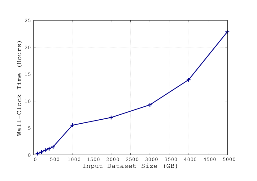
Figure 3.1: Overall Execution Time for Optimisation

3.4.4 Execution Time Analysis

Figure 3.1 shows how the overall optimization time grows in relation to the input size. Table 3.1 illustrates the CPU time usage, which is useful to understand how the I/O latency contributes to the overall execution time of our data-intensive algorithm.

Results from both Figure 3.1 and Table 3.1 indicate two significant outcomes. Firstly, that our method is indeed capable of optimising datasets of disturbance traces that far exceed the available amount of RAM. Secondly, that the performance decreases at a reasonable rate, whereas input data grows at a significant rate with respect to the amount of RAM used for buffering.

Figure 3.2 shows how the sorting step is significantly more time-consuming than all the others. In fact, it takes as long as 12 hours to order the 4-TB input dataset, 6 times longer than the other steps put together.

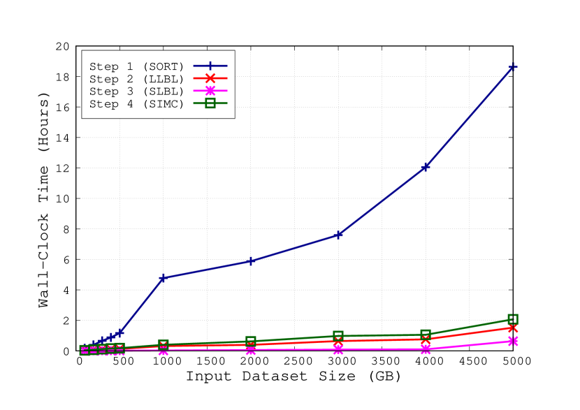
Figure 3.2: Execution Time for each Optimisation Step

Input (GB)	WC Time (sec)	Usr Time (sec)	Sys Time (sec)	CPU Perc. (%)
100	869.96	256.97	208.19	53
200	1888.34	529.17	446.13	52
300	3123.07	807.58	728.63	49
400	4154.61	1082.31	1015.12	50
500	5330.37	1375.38	1346.83	51
1000	19860.45	2905.38	3056.02	30
2000	24998.79	6870.06	6922.10	55
3000	33479.43	9524.09	10505.79	60
4000	50248.18	12533.62	14587.52	54
5000	82325.26	17199.34	20858.58	46

Table 3.1: Overall Execution Time and CPU usage for Optimisation

3.4.5 Optimisation Effectiveness Analysis

In this section we evaluate the effectiveness of our presented optimisation method by analysing results from our benchmark. In particular, we show how much redundant simulation can be removed for each input dataset. To this end, we analyse the number of simulation intervals in both the input scenarios and the resulting simulation campaigns.

Figure 3.3 and Table 3.2 show what we call the Compression Ratio between the input datasets and the resulting optimised simulation campaigns, which we define below.

First, let $SIM(\mathcal{D}):=N\cdot H$ be the number of simulation intervals in a dataset $\mathcal{D}$ that contains $|\mathcal{D}|=N$ input scenarios with horizon $H$. Second, let $SIM(\mathcal{C}):=\sum_{run(t)\text{ }\in\text{ }\mathcal{C}}t$ be the number of simulation intervals in the simulation campaign $\mathcal{C}$ obtained from $\mathcal{D}$, which is the sum of the $t$-arguments of $run(t)$ commands in $\mathcal{C}$. In conclusion, the Compression Ratio between the input dataset and the resulting optimised simulation campaign is $SIM(\mathcal{D})/SIM(\mathcal{C})$.

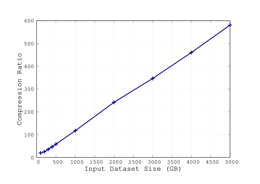
Figure 3.3: Compression Ratio per Input Dataset

Input (GB)	# of Scenarios	$SIM(\mathcal{D})$	$SIM(\mathcal{C})$	Compr. Ratio
100	83333333	12499999950	629628270	19.85
200	166666666	24999999900	994681374	25.13
300	250000000	37500000000	1043778055	35.93
400	333333333	49999999950	1070117781	46.72
500	416666666	62499999900	1067691791	58.54
1000	833330408	124999561200	1065522823	117.31
2000	1666663150	249999472500	1033963170	241.79
3000	2499995861	374999379150	1082233786	346.50
4000	3333326114	499998917100	1086509108	460.19
5000	4166658873	624998830950	1076531113	580.57

Table 3.2: Compression Ratio per Input Dataset

3.5 Related Work

A method to compute optimised simulation campaigns from datasets of scenarios has already been presented in [2]. The idea for this method was based on the presence of labelled lexicographically ordered datasets of input scenarios. In particular, it exploited such an input format in order to efficiently build a Labels Branching Tree (LBT) data structure. The final simulation campaign was then computed from the LBT, which fitted entirely in RAM.

As a result, the method in [2] did not address the computation of labels, and also did not perform the ordering of input scenarios.

In contrast, the method presented in this chapter can efficiently compute simulation campaigns from large datasets of scenarios that are neither labelled nor ordered, and that cannot be fully accommodated into the main memory.

3.6 Conclusions

In this chapter, we presented a method to increase the performance of System-Level Formal Verification (SLFV) by computing highly optimised simulation campaigns from existing datasets that contain a huge number of scenarios that do not fit entirely into the main memory.

For this purpose, we devised and implemented a data-intensive algorithm to efficiently perform the optimisation of such datasets.

In fact, results show that a 4 TB dataset of scenarios can be optimised in as little as 12 hours using just one processor with 50 GB of RAM.

Chapter 4 Execution Time Estimation of Simulation Campaigns

4.1 Introduction

4.1.1 Framework

Simulation Based Verification (SBV) is currently the most widely used approach to carry out System-Level Formal Verification (SLFV) for complex Cyber-Physical Systems (CPSs). In order to perform SBV, it is necessary to execute simulation campaigns on the CPS model to be verified.

Simulation campaigns consist of sequences of simulator commands that are aimed at reproducing all the relevant disturbance sequences (i.e., scenarios) originating from the environment in which the CPS model should operate safely.

Indeed, the goal of SLFV is to prove that the system as a whole is able to safely interact within this environment. For this reason, simulation campaigns include commands to inject the model with disturbances, which represent exogenous events such as hardware failures and system parameter changes.

An example of a simulation campaign could have the following sequence of instructions: (i) simulate the model for 3 seconds, (ii) inject the model with a disturbance, (iii) simulate the model for other 5 seconds, and (iv) check if the state of the model violates any given requirement.

Simulation campaigns are either written by verification engineers or automatically generated from a formal specification model [2]. In this latter case, simulation campaigns can contain as many as $10^{8}$ of simulator commands, which are stored in large binary files of up to hundreds of gigabytes.

As a result of this specification model, simulation campaigns are generated so that SLFV can be performed using an assume-guarantee approach. Namely, a successful SBV process can guarantee that the CPS will behave as expected, assuming that all and only the relevant scenarios are formally specified.

4.1.2 Motivations

Simulation campaigns necessitate a large number of simulator instructions, consequently the length of execution time required to perform SBV tends to be considerable. For example, as illustrated in  [2] it takes as long as 29 days to run a middle-sized simulation campaign for the Fuel Control System model with one 8-core machine (see also [3][4][5]). This makes SBV an extremely time-consuming process, and therefore not very cost effective.

This is mitigated by involving multiple simulators working simultaneously, in the form of clusters that have hundreds of nodes and thousands of cores. For example, results in [4] show that by using 64 machines with an 8-core processor each, the SLFV activity can be completed in about 27 hours whereas a sequential approach would require more than 200 days.

However, there are still the following obstacles to effective SLFV, that involve the management of computing resources. In particular, clusters used to perform SBV are either controlled by commercial companies, thus subjected to strict price policies, or by community based research institutions such as the CINECA, that offer free computation hours for research activities.

Both these kinds of clusters are typically constrained by:

1. The number of cores per task that can be used;

2. The amount of computation hours that can be used.

As a result, it is necessary to either manage the number of cores used to reduce costs, or make the most of the limited number of free computational hours available. Furthermore, each verification phase typically has a strict deadline to be met in order to shorten the time-to-market.

An accurate execution time estimate can reveal if given deadlines can be met. If not, mitigating actions can be taken in good time. For example, the process could be limited to a subset of the simulation campaign. Another option would be to buy additional cores to execute the entire simulation campaign faster.

On top of that, a prior knowledge of the estimated execution time for a simulation campaign helps in calculating the number of cores and computation hours to be bought according to the given time schedule and budget. For example, it is helpful in deciding how many slices to split the simulation campaign into according to the given constraints.

In short, an accurate estimate of execution time leads to better planning of deadlines, and wiser budget allocation for the required computing resources.

4.1.3 Contributions

In order to overcome the lack of tools to perform an effective estimation, we show a method that uses just a small number of execution time samples to accurately train a prediction model. In particular, we describe both how we define our prediction model, and how we choose simulator instructions to collect execution time samples.

This method brings two significant advantages.

First, that only a very small number of execution time samples are required in order to train the prediction model, thus removing the need to simulate a large simulation campaign. Consequently the estimation process is faster, and it is easier to make decisions about the number of slices to split the campaign into (i.e., how many machine to use in parallel).

Secondly, the approach we use to select which simulator commands to sample is machine-independent. Namely, decisions are made on the basis of the simulation model and the solver of the simulator. This makes it possible to select the simulator commands to train the prediction model regardless of the machine where the simulation campaign will run. As a result, we can select commands to sample only once and reuse them to train prediction models on each different machine in the cluster.

To the best of our knowledge, there are no other applicable methodologies in the literature.

4.2 Background

In this section we provide some basic definitions that will be used in the rest of the chapter.

4.2.1 Definitions

Simulation Model

Definition 4.2.1 (Simulation Model).

A simulation model (or simply model) $\mathcal{M}$ is a formal description of the Cyber-Physical System (CPS) to verify (e.g., the Fuel Control System). In particular, the model is written in the language of the simulator being used.

Simulator

Definition 4.2.2 (Simulator).

A simulator $\sigma$ is a software tool that is able to simulate the behaviour of the given CPS model $\mathcal{M}$ to verify.

Set of Disturbances

Definition 4.2.3 (Set of Disturbances).

A set of disturbances $D_{\mathcal{M}}$ is a finite set of disturbances to inject into the CPS model $\mathcal{M}$ during the simulation. Typically, each disturbance $d\in D_{\mathcal{M}}$ consists in modifying some system parameters by the corresponding simulator command $inject(d)$.

Simulation Setting

Definition 4.2.4 (Simulation Setting).

A simulation setting $\mathcal{S}=(\sigma,\mathcal{M},D_{\mathcal{M}},\mu)$ identifies the simulator $\sigma$, the model $\mathcal{M}$ to simulate, the set of disturbances $D_{\mathcal{M}}$ to inject, and the machine $\mu$ where the simulator operates.

4.2.2 Prediction Function

Here we define prediction functions and constants used to estimate the execution time of each command in a simulation campaign $\mathcal{C}$ for a given simulation setting $\mathcal{S}$.

Function $run_{\mathcal{S}}:\mathbb{N}^{+}\rightarrow\mathbb{R}^{+}$ represents the execution time estimate of command $run(t)$ in the setting $\mathcal{S}$. Namely, $run_{\mathcal{S}}(t)$ is the execution time that the simulator takes to advance the state of the model by $\tau\cdot t$ simulation seconds.

Constants $inject_{\mathcal{S}}$, $store_{\mathcal{S}}$, $load_{\mathcal{S}}$, $free_{\mathcal{S}}\in\mathbb{R}^{+}$ represent the execution time estimate of commands inject, store, load, and free, in the same setting $\mathcal{S}$.

Based on a simulation setting $\mathcal{S}$, a simulation campaign $\mathcal{C}$, and a command $c\in\mathcal{C}$, we define as follows our prediction function $\mathcal{P}_{\mathcal{S}}(c)$ to indicate the execution time estimate for command $c$ in the simulation setting $\mathcal{S}$.

$$\mathcal{P}_{\mathcal{S}}(c)=\left\{\begin{array}[]{ll}run_{\mathcal{S}}(t)&c=run(t),t\in\mathbb{N}^{+}\\ inject_{\mathcal{S}}&c=inject(d),d\in D_{\mathcal{M}}\\ store_{\mathcal{S}}&c=store(s),s\in\mathbb{N}^{+}\\ load_{\mathcal{S}}&c=load(s),s\in\mathbb{N}^{+}\\ free_{\mathcal{S}}&c=free(s),s\in\mathbb{N}^{+}\\ \end{array}\right.$$

4.3 Problem Formulation

Let be given a simulation setting $\mathcal{S}$ and a simulation campaign $\mathcal{C}$. The aim is to automatically find an accurate estimation of the execution time to simulate $\mathcal{C}$ in the simulation setting $\mathcal{S}$ by training our prediction function $\mathcal{P}_{\mathcal{S}}$ in such a way that the resulting estimate $\mathcal{P}^{\mathcal{C}}_{\mathcal{S}}$ is the sum of the estimates for each simulator command $c$ in $\mathcal{C}$, i.e.,

$$\mathcal{P}^{\mathcal{C}}_{\mathcal{S}}=\sum_{c\text{ }\in\text{ }\mathcal{C}}\mathcal{P}_{\mathcal{S}}(c).$$

In the rest of the chapter we show how we effectively train $\mathcal{P}_{\mathcal{S}}$ and how we validate its accuracy.

4.4 Methodology

Given how useful having an execution time estimate is, it would be tempting to compute it on the basis of an existing simulation campaign. Once collected, the execution time samples would be used to train a prediction model. However, this naïve approach is risky as it could potentially lead to either poor performances or to inaccurate results for the following reasons. First, the given simulation campaign may require hours of simulations. Second, if a relatively small subset of the given campaign is used, the resulting collected samples could be either insufficient or inappropriate to train an accurate prediction model.

As an example, let us consider only the command $run(t)$, which is the most expensive from a computational point of view. It would be natural to assume a linear relationship between the execution time $e_{run}(t)$ to actually simulate it, and the number of simulation seconds $\tau\cdot t$ that are required to advance. Namely, the estimated execution time to simulate $run(t)$ would be $e_{run}(t):=a\cdot t+b$.

To train such a simple prediction model, a careful selection of $t$-values to sample is needed, according to the following phenomena we observed on several Simulink models.

First, for small values of $t$ up to a certain value $t_{min}$, the execution time to simulate $run(t)$ remains reasonably constant or it grows at a very low rate. Second, for large values of $t$ from a certain value $t_{MAX}$, the execution time grows constantly and it is strictly related to the number of numerical integration steps performed by the simulator. Clearly, $t_{min}$ and $t_{MAX}$ vary depending on the complexity of the model being simulated.

Note that a typical simulation campaign includes a large number of $run(t)$ commands with both short and long values of $t$. These last observations together constitute the main reason why the aforementioned naïve approach would lead to inaccurate estimates, if execution time samples are not collected properly.

4.4.1 Overall Method

In order to train our prediction function $\mathcal{P}_{\mathcal{S}}$, we use a small number of execution time samples that are sufficient to make an accurate execution time estimate of a given simulation campaign $\mathcal{C}$. To this end, we collect such samples by simulating an ad-hoc sequence $\mathcal{C}^{*}$ of simulator commands that we choose for this purpose.

More precisely, we proceed as follows. First, we accurately choose simulator commands to put in $\mathcal{C}^{*}$ in order to compute a meaningful training set. Second, we simulate $\mathcal{C}^{*}$ to collect execution time samples in our training set. Finally, we use the resulting training set to compute parameters for our prediction function $\mathcal{P}_{\mathcal{S}}$.

In the following sections we show how we build $\mathcal{C}^{*}$ and more specifically which $t$-values we choose to collect execution time samples of $run(t)$ commands.

4.4.2 Training Phase

When working with Simulink, if we simulate a command $run(t)$ multiple times with the same $t$-value on a model $\mathcal{M}$, then the solver always chooses the same numerical integration steps, hence the number of such steps remains unchanged (Figure 4.1). Clearly, this stability is not reflected in the resulting execution time when we simulate the same command $run(t)$ multiple times with the same $t$-values (Figure 4.2).

Note that Figure 4.1 and Figure 4.2 are similar in that they are almost constant for $t\leq 1$ and they linearly grow for $t>1$. This similarity can be explained by the fact that the execution time the simulator needs is strictly related to the numerical integration steps it performs. Also note that the breakpoint at $1$ in these figures is strictly linked to the model $\mathcal{M}$ being simulated, which is the Fuel Control System in this case.

Based on the above considerations, we define our prediction function $run_{\mathcal{S}}$ that estimates the execution time needed to simulate $run(t)$ as the following 2-step Piecewise Linear Function (PWLF).

$$run_{\mathcal{S}}(t):=\left\{\begin{array}[]{lr}\alpha&t\leq\gamma\\ \beta\cdot(t-\gamma)+\alpha&t\geq\gamma\\ \end{array}\right.$$

In order to train this function, we first collect execution time samples of $run(t)$ commands, and then we use these samples to find the intercept $\alpha$, the slope $\beta$, and the breakpoint $\gamma$ of $run_{\mathcal{S}}$.

In the following section we illustrate how we choose these $t$-values by analysing the integration steps that the simulator performs for each $t$-value.

Set of $t$-values $T_{\mathcal{M}}$

The aim is to select a set $T_{\mathcal{M}}$ with the $t$-values of $run(t)$ commands to simulate in order to collect meaningful training data for our prediction function $run_{\mathcal{S}}$. In particular, we need to collect execution time samples of $run(t)$ commands for either short or long $t$-values.

To this end, we first find two values $t^{min}_{\mathcal{M}}$ and $t^{MAX}_{\mathcal{M}}$, that correspond to the minimum and the maximum $t$-values in $T_{\mathcal{M}}$ respectively.

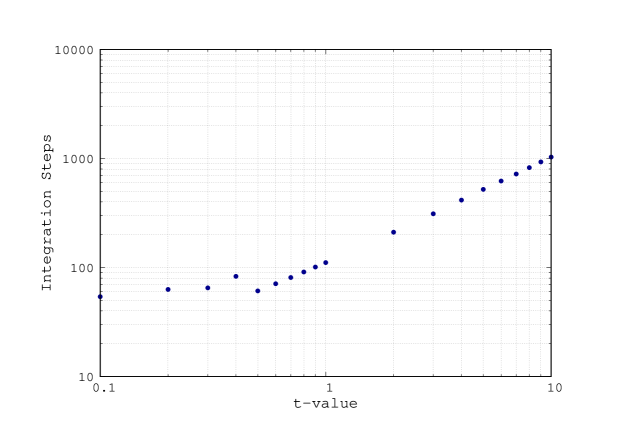
Figure 4.1: Integration Steps to Simulate Command $run(t)$

Figure 4.2: Execution Time to Simulate Command $run(t)$

Let define $N_{\mathcal{M}}(t)$ as the number of integraton steps that the simulator performs to simulate $run(t)$ on the model $\mathcal{M}$. Our method to find $t^{min}_{\mathcal{M}}$ and $t^{MAX}_{\mathcal{M}}$ exploits these two key observations: (i) for small $t$-values, the execution time to simulate $run(t)$ remains relatively constant, i.e., $run_{\mathcal{S}}(t)\simeq c_{1}$, for $t<t^{min}_{\mathcal{M}}$, and (ii) for large $t$-values, it grows constantly and it is strictly related to the number $N_{\mathcal{M}}(t)$ of integration steps, i.e., $run_{\mathcal{S}}(t)\simeq N_{\mathcal{M}}(t)\cdot c_{2}$, for $t>t^{MAX}_{\mathcal{M}}$.

To find $t^{min}_{\mathcal{M}}$, we use the Algorithm 2, which works in the following way. Basically, we search for the largest interval $(0,t^{min}_{\mathcal{M}})$ of all the $t$-values for which the number $N_{\mathcal{M}}(t)$ of steps performed to simulate $run(t)$ remains constant. Note that for $t$-values that are close to zero, the simulator performs the same number $N_{\mathcal{M}}(t)$ of integration steps. For these reasons, in order to train $run_{\mathcal{S}}(t)$ it is sufficient to choose $t^{min}_{\mathcal{M}}$ as the greatest $t$-value such that $N_{\mathcal{M}}(t)$ remains constant for every $t^{\prime}$ less than or equal to $t^{min}_{\mathcal{M}}$, i.e.,

$$t^{min}_{\mathcal{M}}=\max\{t\;|\;(\forall t^{\prime}\leq t)(N_{\mathcal{M}}(t)=N_{\mathcal{M}}(t^{\prime}))\}.$$

Once we have selected the lower bound $t^{min}_{\mathcal{M}}$ of $T_{\mathcal{M}}$, we look for the smallest upper bound $t^{MAX}_{\mathcal{M}}$ in order to make the final training set as small as possible, thus minimising the training effort.

To find $t^{MAX}_{\mathcal{M}}$, we use the Algorithm 3. As mentioned, the function $N_{\mathcal{M}}(t)$ is relatively constant for small $t$-values, while it linearly grows for the larger ones. For this reason, the value of $t^{MAX}_{\mathcal{M}}$, is the smallest $t$ such that the linear regression on the collected points in $(t^{min}_{\mathcal{M}},t]$ has an error lower than a given bound $\varepsilon$.

Input: Model $\mathcal{M}$.

Output: $t^{min}_{\mathcal{M}}\in\mathbb{R}^{+}$.

1 $N_{0}\leftarrow N_{\mathcal{M}}(10^{0})$;

2 for each $i\leftarrow-1,-2,-3,\ldots$ do

3       $N_{i}\leftarrow N_{\mathcal{M}}(10^{i}))$;

4       if $N_{i}=N_{i+1}$ then

5             exit for;

6            

7       end if

8      

9 end for

10$t^{min}_{\mathcal{M}}\leftarrow 10^{i+1}$;

Algorithm 2 Find $t^{min}_{\mathcal{M}}$.

Input: Model $\mathcal{M}$; $t^{min}_{\mathcal{M}}\in\mathbb{R}^{+}$; $\varepsilon$.

Output: $t^{MAX}_{\mathcal{M}}\in\mathbb{R}^{+}$.

1 for each $i\leftarrow 1,2,3,\ldots$ do

2       $t_{i}\leftarrow t^{min}_{\mathcal{M}}\cdot 10^{i-1}$;

3       $N_{i}\leftarrow N_{\mathcal{M}}(t_{i})$;

4       if $i\geq 3$ then

5             $\tilde{N}_{i}\leftarrow\alpha+\beta\cdot t_{i}$, where $\alpha$ and $\beta$ are linear regression coefficients computed from a set of samples $(t_{j},N_{j})$ collected at previous iterations, with $j=1,2,\ldots,i-1$;

6             if $|\frac{N_{i}}{\tilde{N}_{i}}-1|<\varepsilon$ then

7                   exit for;

8                  

9             end if

10            

11       end if

12      

13 end for

14$t^{MAX}_{\mathcal{M}}\leftarrow t_{i}$;

Algorithm 3 Find $t^{MAX}_{\mathcal{M}}$.

From $t^{min}_{\mathcal{M}}$ and $t^{MAX}_{\mathcal{M}}$, we can finally define our set of $t$-values as the following. Let $a$ and $b$ be such that $t^{min}_{\mathcal{M}}=10^{a}$ and $t^{MAX}_{\mathcal{M}}=10^{b}$ respectively.

$$T_{\mathcal{M}}:=\bigcup^{b-1}_{i=a}\bigcup^{10}_{j=1}\{10^{i}\cdot j\}.$$

Namely, we put in $T_{\mathcal{M}}$ $10$ equidistant $t$-values from all the subranges $[10^{i},10^{i+1}]$ in the range $[t^{min}_{\mathcal{M}},t^{MAX}_{\mathcal{M}}]$, with $i=a,a+1,\ldots,b-1$.

Table 4.1 shows the values $t^{min}_{\mathcal{M}}$ and $t^{MAX}_{\mathcal{M}}$ found by the Algorithm 2 and the Algorithm 3 including the error $\varepsilon$ used by the Algorithm 3, and the resulting total number $|T_{\mathcal{M}}|$ of $t$-values to sample, for each Simulink model.

Note that the computation of $T_{\mathcal{M}}$ is machine-independent. In fact, the information we use to find $t^{min}_{\mathcal{M}}$ and $t^{MAX}_{\mathcal{M}}$ depends only on the given model $\mathcal{M}$ and the simulator solver.

Model $\mathcal{M}$	$t^{min}_{\mathcal{M}}$	$t^{MAX}_{\mathcal{M}}$	$\varepsilon$	$|T_{\mathcal{M}}|$
sldemo_fuelsys.mdl	$10^{-2}$	$10^{3}$	$10^{-2}$	$46$
aero_dap3dof.slx	$10^{-4}$	$10^{2}$	$10^{-2}$	$55$
penddemo.slx	$10^{-6}$	$10^{2}$	$10^{-2}$	$73$
sldemo_boiler.slx	$10^{1}$	$10^{5}$	$10^{-2}$	$37$
sldemo_engine.slx	$10^{-5}$	$10^{4}$	$10^{-2}$	$82$
sldemo_househeat.slx	$10^{-1}$	$10^{4}$	$10^{-2}$	$46$

Table 4.1: Values of $t$ to Sample for Command $run(t)$

Simulation Campaign $\mathcal{C}^{*}$

From the set $T_{\mathcal{M}}$ of $t$-values, we populate the sequence $\mathcal{C}^{*}$ of simulator commands. In particular, this sequence is made up of commands $inject(d)$ and $run(t)$, for each $t\in T_{\mathcal{M}}$, and for each disturbance $d\in D_{\mathcal{M}}$. On top of that, we populate $\mathcal{C}^{*}$ with commands load, store, and free in a consistent way. Namely, commands $load(x)$ and $free(x)$ are preceded by the corresponding command $store(x)$.

Once our simulation campaign $\mathcal{C}^{*}$ is ready, we use it to populate our training set with execution time samples. To this end, we simulate $\mathcal{C}^{*}$ multiple times in order to collect a meaningful number of training samples.

4.4.3 Prediction Function

Command Run

In order to train our prediction function $run_{\mathcal{S}}$, we proceed in the following way. Our training set $S_{\mathcal{M}}:=(S_{1},S_{2},\ldots,S_{N})$ contains those samples collected from simulating $run(t)$ commands in the simulation campaign $\mathcal{C}^{*}$. Namely, each $S_{i}=(t_{i},\tau_{i})$, with $i\in[N]$, is a pair that contains the measured execution time $\tau_{i}$ to simulate $run(t_{i})$ on the model $\mathcal{M}$, with $t_{i}\in T_{\mathcal{M}}$.

As previously shown, the shape of our prediction function $run_{\mathcal{S}}$ is a PWLF with breakpoint in $\gamma$, i.e.,

$$run_{\mathcal{S}}(t):=\left\{\begin{array}[]{lr}\alpha&t\leq\gamma\\ \beta\cdot(t-\gamma)+\alpha&t\geq\gamma\\ \end{array}\right.$$ (4.1)

In order to train this function $run_{\mathcal{S}}(t)$, we search for those parameters $\alpha$, $\beta$, and $\gamma$ in 4.1 that minimise the percentage Root-Mean-Square Error (RMSE) on both the following sets.

Let $S_{\mathcal{M}}^{t<\gamma}:=\{(t_{i},\tau_{i})\in S_{\mathcal{M}}:t<\gamma\}$ be the subset of $S_{\mathcal{M}}$ with $t$-values less than $\gamma$. Similarly, let $S_{\mathcal{M}}^{t\geq\gamma}:=\{(t_{i},\tau_{i})\in S_{\mathcal{M}}:t\geq\gamma\}$ be the subset of $S_{\mathcal{M}}$ with $t$-values greater or equal to $\gamma$. We search for $\alpha$, $\beta$, and $\gamma$ that minimise the following sum.

$$Err_{S_{\mathcal{M}}}=\sum_{S\in\{\{S_{\mathcal{M}}^{t<\gamma}\},\{S_{\mathcal{M}}^{t\geq\gamma}\}\}}\sqrt{\frac{1}{|S|}\sum_{(t_{i},\tau_{i})\in S}\left(\frac{\tau_{i}-run_{\mathcal{S}}(t_{i})}{\tau_{i}}\right)^{2}}$$ (4.2)

To this end, we use the CPLEX Optimiser. In particular, we iterate over different chosen values of $\gamma$, and let CPLEX decide the values of $\alpha$ and $\beta$ that minimise $Err_{S_{\mathcal{M}}}$ for the given $\gamma$. Finally, we choose those $\alpha$ and $\beta$ associated to the $\gamma$ with the minimum resulting $Err_{S_{\mathcal{M}}}$.

Table 4.2 shows the values $\alpha$, $\beta$, and $\gamma$ found using the training set $S_{\mathcal{M}}$, and the percentage RMSE $Err_{S_{\mathcal{M}}}$ associated to the function $run_{\mathcal{S}}$ for each Simulink model.

Model $\mathcal{M}$	$\alpha$	$\beta$	$\gamma$	$Err_{S_{\mathcal{M}}}$
sldemo_fuelsys.mdl	$0.39$	$0.02$	$0.4$	$2.8\%$
aero_dap3dof.slx	$0.39$	$0.04$	$0.1$	$3.8\%$
penddemo.slx	$0.038$	$0.0014$	$10$	$23.0\%$
sldemo_boiler.slx	$0.1$	$2\times 10^{-5}$	$50$	$7.6\%$
sldemo_engine.slx	$0.04$	$0.01$	$1.22$	$2.0\%$
sldemo_househeat.slx	$0.08$	$0.0001$	$10$	$8.9\%$

Table 4.2: Parameters of Prediction Function $run_{\mathcal{S}}$

Other Commands

Finally, we train our constants $load_{\mathcal{S}}$, $store_{\mathcal{S}}$, $free_{\mathcal{S}}$, and $inject_{\mathcal{S}}$ that we need to define our final prediction function $\mathcal{P}^{\mathcal{C}}_{\mathcal{S}}$. To this end, we compute the average execution time for each type of simulator command from the collected samples. In particular, we set each prediction constant with the average execution time of the corresponding simulator command.

For example, let $S^{inject}_{\mathcal{M}}:=(\tau_{1},\tau_{2},\ldots,\tau_{K})$ be a training set that contains $K$ execution time samples collected by simulating inject commands in $\mathcal{C}^{*}$. We define our constant $inject_{\mathcal{S}}$ as the average execution time of the gathered samples in $S^{inject}_{\mathcal{M}}$. Namely,

$$inject_{\mathcal{S}}:=\frac{1}{|S^{inject}_{\mathcal{M}}|}\sum_{i\in[K]}\tau_{i}.$$

We do the same thing to train the other constants $load_{\mathcal{S}}$, $store_{\mathcal{S}}$, and $free_{\mathcal{S}}$ in $\mathcal{P}^{\mathcal{C}}_{\mathcal{S}}$.

The reason why we choose constants to estimate the execution time of these simulator commands is clearly shown in Figures 4.5, 4.4, 4.3, and 4.6. These figures show the distribution of the execution time samples of the corresponding simulator commands, that we collected by simulating $\mathcal{C}^{*}$ on the Fuel Control System model.

As an example, from Figure 4.5 we see that the execution time to simulate commands $inject(d)$ in $\mathcal{C}^{*}$ is mostly between 0.5 and 0.6 seconds.

In conclusion, Figure 4.7 shows the average and standard deviation of the execution time to run commands load, store, inject, and free, on each Simulink model we used for our experiments.

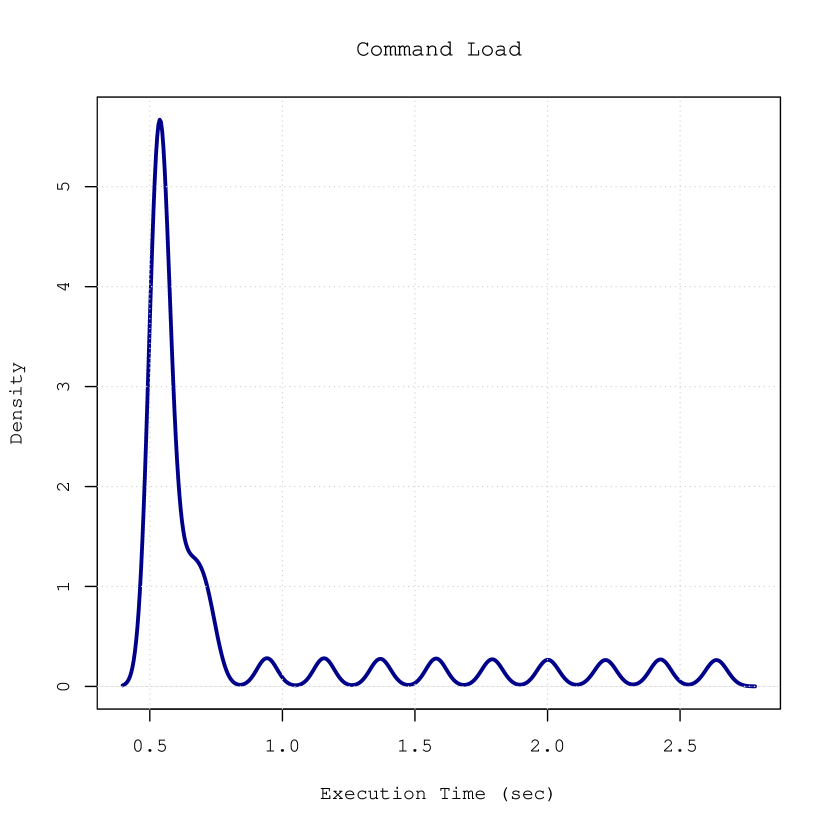
Figure 4.3: Execution Time Distribution of Command load

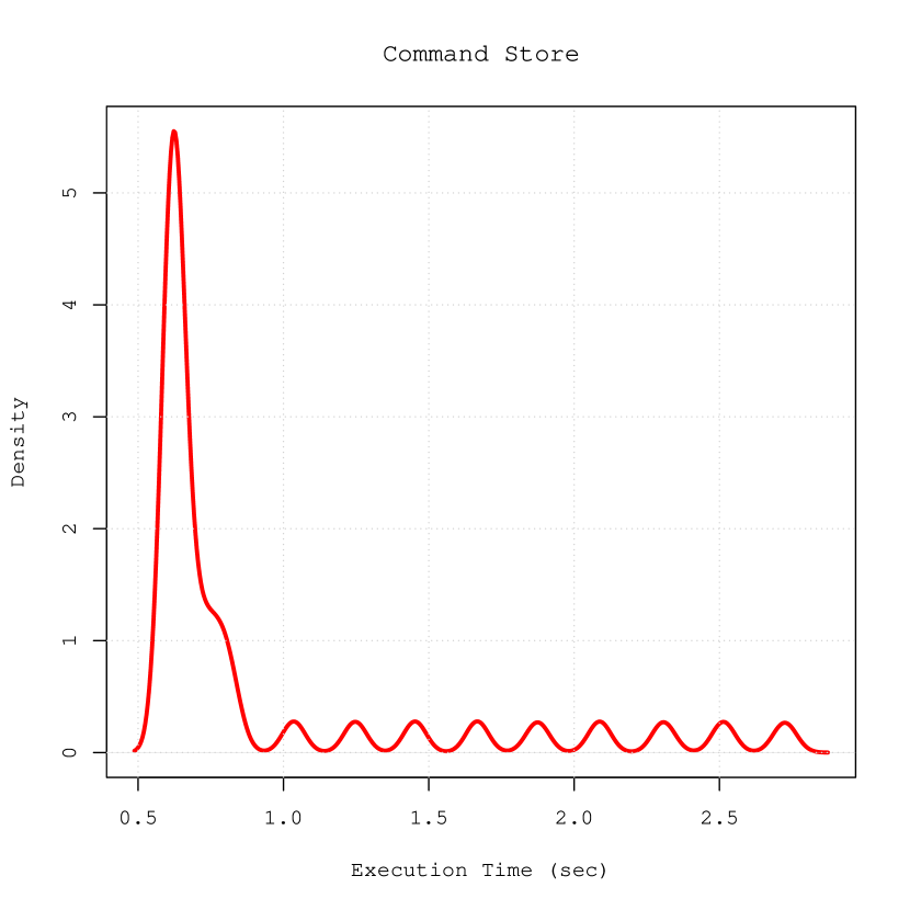
Figure 4.4: Execution Time Distribution of Command store

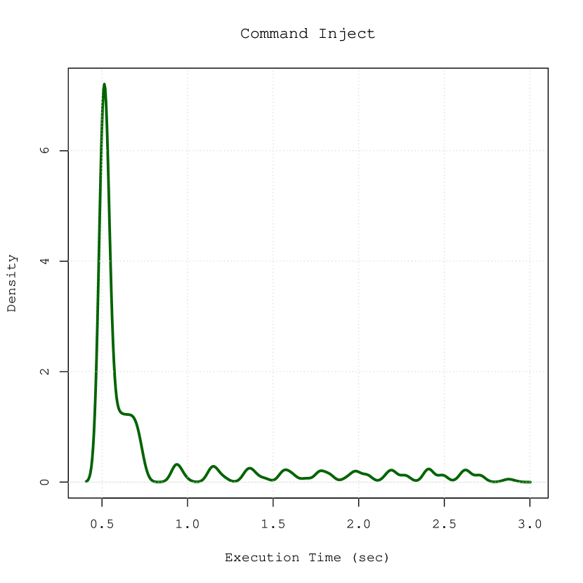
Figure 4.5: Execution Time Distribution of Command inject

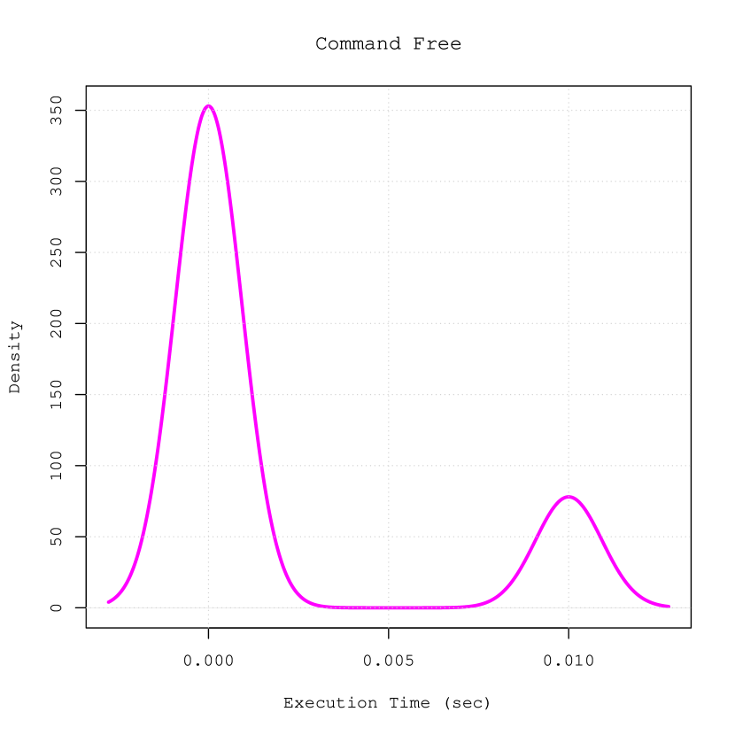
Figure 4.6: Execution Time Distribution of Command free

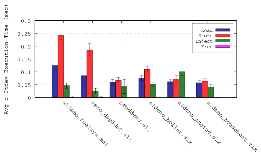
Figure 4.7: Execution Time for Commands load, store, inject, and free

4.5 Experimental Results

4.5.1 Validation of the Method

Command Run

Our goal is to validate the accuracy of the execution time estimate $run_{\mathcal{S}}(t)$ for any $t\in\mathbb{R}^{+}$. For this reason, we specifically build a validation set for our prediction function $run_{\mathcal{S}}$ in the following way. We define this set as $V^{run}_{\mathcal{M}}:=\cup_{i=1}^{K}V_{i}$, where each $V_{i}$ is

$$V_{i}:=\bigcup_{t\in T_{\mathcal{M}}}\{(t^{\prime},\tau)\}\text{, with }t^{\prime}\in[t\div 10,t\cdot 10].$$

Namely, we populate a meaningful number $K$ of validation sets $V_{i}$ by collecting execution time samples of $run(t)$ commands on the model $\mathcal{M}$. In particular, we choose $t^{\prime}$-values in each sample $(t^{\prime},\tau)$ by picking a random value from the interval $[t\div 10,t\cdot 10]$, for every $t\in T_{\mathcal{M}}$.

Finally, we compute the prediction error of our function $run_{\mathcal{S}}$ as the average relative error between the measured execution time and the estimated one. Namely,

$$Err_{run_{\mathcal{S}}}:=\frac{1}{|V^{run}_{\mathcal{M}}|}\sum_{(t,\tau)\in V^{run}_{\mathcal{M}}}\frac{|\tau-run_{\mathcal{S}}(x)|}{\tau}.$$

Figure 4.8 and Table 4.3 show the average of the prediction errors found on each validation set $V_{i}$. In particular, we obtain these results using $K=100$ validation sets for each Simulink model.

Figure 4.9 shows the distribution of the relative prediction error of function $run_{\mathcal{S}}$ for the Fuel Control System model, computed on the entire validation set $V^{run}_{\mathcal{M}}$.

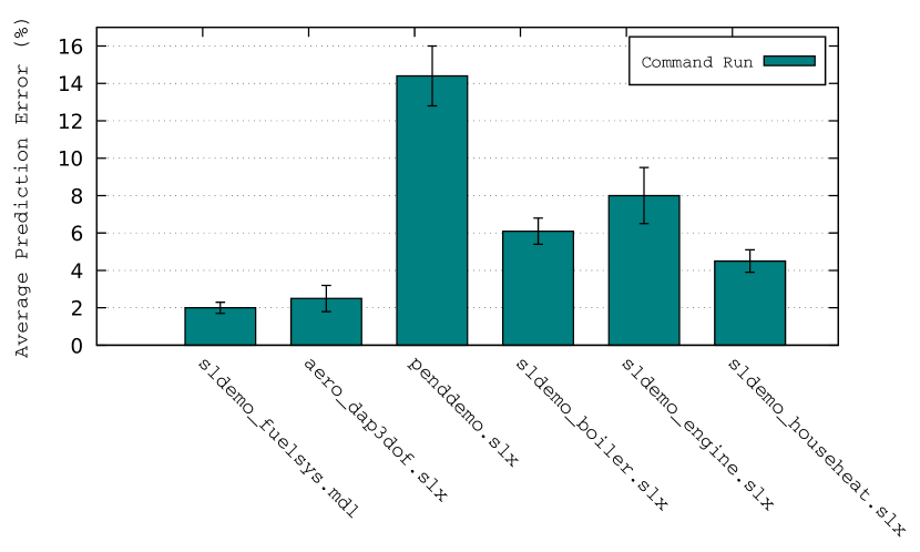
Figure 4.8: Average Prediction Error of $run_{\mathcal{S}}$

Model $\mathcal{M}$	Minimum	Maximum	Average	Standard Deviation
sldemo_fuelsys.mdl	1.1	2.5	2.0	0.3
aero_dap3dof.slx	1.9	5.5	2.5	0.7
penddemo.slx	10.9	18.3	14.4	1.6
sldemo_boiler.slx	3.9	7.6	6.1	0.7
sldemo_engine.slx	5.7	10.6	8.0	1.5
sldemo_househeat.slx	3.4	5.7	4.5	0.6

Table 4.3: Average Prediction Error of $run_{\mathcal{S}}$

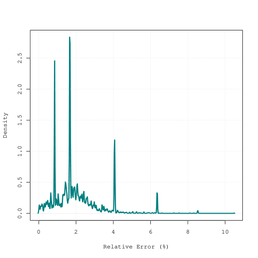
Figure 4.9: Relative Error Distribution of $run_{\mathcal{S}}$

Simulation Campaigns

Slices	Average per Slice (hh:mm:ss)			Relative Error (%)
	Measured	Estim$\alpha\beta\gamma$	Estimnaïve	Err$\alpha\beta\gamma$	Errnaïve
128	96:08:22	99:23:49	99:32:35	7.09	7.07
256	51:36:56	51:38:26	51:49:34	1.29	1.20
512	26:04:26	26:08:05	26:13:25	2.59	2.43

Table 4.4: Estimation Error of Simulation Campaings

Table 4.4 describes the estimation results from our experiments. It illustrates both the measured and estimated execution time to simulate slices of simulation scenarios. These slices are obtained from a dataset of scenarios that we generated automatically from a formal model of disturbances to verify the Apollo Simulink model.

To perform these experiments, we first split the initial dataset of scenarios into 128, 256, and 512 slices. Then, from these slices we compute the corresponding optimised simulation campaigns. Finally, we execute each simulation campaign in parallel, and collect the elapsed time of the simulation.

Results from Table 4.4 show that the measured elapsed time to run a simulation campaign from the 128-slice group is around 96 hours on average. The corresponding elapsed time estimated with both our presented methods (i.e., Estim_{$\alpha\beta\gamma$}) and the naïve one (i.e., Estim_naïve) is around 99 hours on average, with an error of approximately 7%.

It is worth noting that the naïve estimation was obtained from execution time samples collected by running an entire simulation campaign from the 128-slice group. The execution of this campaign as a whole required around 96 hours of simulation.

In contrast, our estimation was obtained from just a few execution time samples collected by running a small simulation campaign we computed ad-hoc. In particular, this simulation campaign is made of about 100 simulator instructions. As can be seen, the execution of this campaign was significantly shorter and is measured in terms of minutes, rather than hours. In fact the total amount of time required was a mere 10 minutes of simulation.

4.6 Related Work

To the best of our knowledge, no previous work in the literature directly addresses the challenge of estimating the execution time of simulation campaigns [6]. In fact, when cluster usage is limited to a maximum walltime $w$ for computation tasks, the typical workaround used for computations requiring more than $w$ seconds is called checkpointing [8]. Namely, the computation task must periodically save its state (checkpoint). In this way, if the task is killed–either because the walltime has expired, or because the cluster has faulted [8]–it may be restarted from the last checkpoint rather than from the beginning.

The use of checkpointing is not appropriate in our setting for the following reasons: (1) The application code must be instrumented in order to perform checkpointing. Although this is leveraged by existing software libraries [1], it requires both access to and knowledge of the source code, which may not be possible. (2) Checkpointing does not provide trade-off between computational resources and splitting of simulation campaigns into smaller or bigger slices, which is our focus here.

With regard to hardware/software Worst Case Execution Time (WCET), some research has been done on studying algorithms and methods to estimate it. As an example, in [7] a systematic method is presented that makes model information available for timing analysis and presents promising results with Simulink/Stateflow models.

In [9] an approach based on integer linear programming is presented for calculating a WCET estimate from a given database of timed execution traces.

The main differences between estimation of WCET and estimation of the execution time of simulation campaigns are the following: (1) WCET aims to determine the worst scenario of execution of a system, mainly to check that hard real-time requirements in hardware/software interactions are met. On the other hand, our focus here is on the average execution time of a simulation campaign. (2) WCET is typically tailored to some specific hardware architecture. On the contrary, our method targets any computer architecture, as it also contains a hardware-dependent training phase.

4.7 Conclusions and Future Work

4.7.1 Conclusions

In this chapter, we presented an effective method to perform an accurate execution time estimate of simulation campaigns. In particular, we described our machine-independent approach to selecting a small number of simulators commands to collect execution time samples from. Furthermore, we showed how to train a prediction function from the collected samples.

Results show that our method can effectively predict the time needed to execute a simulation campaign with an error below 10%.

Chapter 5 Conclusions and Future Work

5.1 Conclusions

In this thesis, we have presented an optimiser and an execution time estimator employed to overcome the limitations associated with Model Based System-Level Formal Verification (SLFV) tools for complex Cyber-Physical Systems (CPSs). Namely the significant amount of time required for simulations as well as the unpredictability of its length, which prevent a more widespread adoption of SLFV tools over the entire development life cycle.

In Chapter 3, we presented an efficient data-intensive optimiser tool to speed up the SLFV process by obtaining optimised simulation campaigns from the existing datasets of scenarios to be verified. Optimised simulation campaigns accelerate SBV by exploiting the capability of modern simulators to store and re-use intermediate simulation states in order to eliminate the need to explore common paths of scenarios multiple times.

In Chapter 4, we presented an effective partially machine-independent execution time estimator tool to predict the required time to complete SLFV activities. An accurate estimate of execution time leads to better planning of deadlines, and wiser budget allocation for the required computing resources.

5.2 Future Work

Experimental results in Section 3.4 indicate that our optimisation method could also be scaled horizontally. In fact, Figure 3.2 shows how the sorting step is significantly more time-consuming than all the others. In fact, it takes as much as 12 hours to sort the 4-TB input dataset, 6 times longer than the other steps put together.

For this reason, an interesting further investigation could be to delegate this step to a cluster-computing framework such as Apache Spark in a dedicated cluster. Such an approach has indeed led to very promising results in recent publications. For example, a team from the Apache Spark community showed how they managed to sort 100 TB of data in as little as 23 minutes [10].

Another investigation into the applicability of the optimiser tool would be the optimisation of existing datasets used in CPS companies. This would require the implementation of the following pre-processing step in order to convert existing scenarios into the input format that we use for our optimiser. Faulty events in the existing dataset would be encoded with disturbance IDs (i.e., disturbances). Next, the fixed length $H$ of scenarios that we use in our input format could be obtained from the existing dataset by searching for the largest sequence of disturbances in the same existing dataset. Once $H$ is obtained, all the other scenarios with length less than $H$ in the existing dataset could be expanded by appending to them the appropriate number of zeros (i.e., non-disturbances) in order to make all the resulting scenarios the same length $H$.

Since there is currently a great interest about continuous integration and deployment of new software components in CPSs that are already in use, e.g., new subsystems in vehicles that are already on the road, it would be interesting to investigate on the possibility to use the solutions presented in this thesis together with incremental verification techniques [19] in order to select only those simulation scenarios that are actually needed to be re-verified, according to the performed software changes.

In conclusion, while in this thesis we focused on Simulink to devise our estimation method, it would be interesting to investigate the applicability of our method with other industrially viable simulators such as Ngspice and JModelica. The use of these simulators would require the implementation of two driver tools to translate each simulator command from the simulation campaign into the corresponding instructions to be executed by Ngspice and JModelica. A Simulink implementation of such a driver tool can be found at our Bitbucket repository.

Appendix A Optimiser Tool: Implementation and Usage

In this section we show how we implemented our optimiser tool. In particular, we first illustrate both the input and output format, and then we describe each step of the algorithm.

The implemented code of the presented optimiser tool is available at our Bitbucket repository.

A.1 Definitions

Lex-Ordered Dataset of Disturbance Traces

A lex-ordered dataset of Disturbance Traces (DTs) is an ordered sequence $\mathcal{D}$ that contains $|\mathcal{D}|=N$ distinct DTs with length $H$, i.e.,

$$\mathcal{D}:=\bigcup_{i\in[N]}\{(d^{i}_{1},d^{i}_{2},\ldots,d^{i}_{H})\}.$$

In particular, each disturbance $d^{i}_{j}\in\mathbb{N}^{+}\cup\{0\}$ is a natural number that encodes a fault to inject on the model being simulated. Furthermore, zeros indicate non-disturbances.

Simulation Scenario

Given the $i$-th DT $\delta_{i}=(d^{i}_{1},d^{i}_{2},\ldots,d^{i}_{H})$ in a lex-ordered dataset $\mathcal{D}$, a simulation scenario (or scenario) is a sequence of $H$ consecutive simulation intervals where we inject the model being simulated with each disturbance $d^{i}_{j}\in\delta_{i}$ at the beginning of the corresponding $j$-th interval. Note that if $d^{i}_{j}=0$, then no disturbance is injected. Furthermore, each simulation interval has a fixed length $\tau$ of simulation seconds. In conclusion, we give the name $H$ to the simulation horizon (or horizon).

Simulation Campaign

Given a lex-ordered dataset $\mathcal{D}$ of DTs in input, a simulation campaign is a sequence of simulator commands that are aimed at simulating scenarios in $\mathcal{D}$. Simulator commands are described in Table A.1 below.

Simulator Commands

Table A.1 shows the syntax and behaviour of the five basic simulator commands.

Syntax	Behaviour
I<int>	injects the disturbance <int> on the model being simulated
R<int>	advances the simulator state by <int> simulation intervals
S<int>	saves the current simulator state in a file named <int>
L<int>	loads the simulator state from the file <int>
F<int>	removes the file <int>

Table A.1: Syntax of Simulator Commands

A.2 Input Format

The input file (DT file) is a binary file that contains DTs where disturbances are encoded by unsigned 64-bit integers.

In particular, a DT file contains a multiset of DTs that have horizon $H$, thus DTs are not lex-ordered so there can be duplicate DTs. Furthermore, there is no header in the DT file that indicates the horizon H of DTs. Also, there is no separator between DTs.

Hence, a DT file is a simple sequence of $N\cdot H$ disturbances, where $N$ is the number of DTs in the DT file, and $H$ is their horizon.

Example A.2 (Input File). Below is an example of an input DT file. Specifically, it contains a multiset of DTs with horizon $H=5$. Note that DTs are not lex-ordered and there are duplicate DTs.

For the sake of clarity, the content of the input DT file above is shown in a textual format. Namely, disturbances are shown in their textual representation and are separated by space characters. Furthermore, DTs are separated by new lines.

A.3 Output Format

The output file (optimised simulation campaign) is a text file with simulator commands that are aimed at simulating the corresponding DTs in the input lex-ordered dataset.

Specifically, each line in the optimised simulation campaign (say the $i$-th line) contains simulator commands that simulate the corresponding DT in input (the $i$-th DT in the dataset). Each line has the following syntax.

$$\text{{\tt F}\textless}\text{{\tt int}\textgreater}\{0,H-1\}\text{ }\text{{\tt L}\textless}\text{{\tt int}\textgreater}\{1\}\text{ }(\text{{\tt I}\textless}\text{{\tt int}\textgreater}\{0,1\}\text{ }\text{{\tt R}\textless}\text{{\tt int}\textgreater}\{1\}\text{ }\text{{\tt S}\textless}\text{{\tt int}\textgreater}\{0,1\})\{1,H\}$$

In particular, there can be a number from 0 to $H-1$ of commands free (i.e., F<int>), depending on the current number of previously stored simulation states that are no longer needed by future DTs.

Then, there is the command load (i.e., L<int>). Note that this command is mandatory. In fact, each input DT in the resulting simulation campaign starts from its corresponding initial state. Note that <int> indicates an integer.

Lastly, there is a number from 1 to $H$ of inject-run-store commands (i.e., $\text{{\tt I}\textless}\text{{\tt int}\textgreater}\{0,1\}\text{ }\text{{\tt R}\textless}\text{{\tt int}\textgreater}\{1\}\text{ }\text{{\tt S}\textless}\text{{\tt int}\textgreater}\{0,1\}$), depending on both the number of disturbances to inject and the number of states to store. Specifically, commands inject and store (i.e., I<int>, and S<int>) are optional since there can be neither disturbances to inject nor states to store at certain simulation intervals.

Example A.3 (Output File). Below is an example of an optimised simulation campaign that corresponds to the lex-ordered dataset of input DTs shown in the input file example.

Note that the command L0 loads the initial simulator state, which is assumed to exist prior to the simulation, thus there is no previous S0 command in the simulation campaign.

A.4 Algorithm Steps

Step 1. Initial Sorting

INPUT:

A file that contains a multiset of DTs with length $H$.

OUTPUT:

A file that contains the corresponding lex-ordered dataset $\mathcal{D}$ of DTs.

The output dataset $\mathcal{D}$ is obtained from uniquely sorting the input DTs.

Example A.4.1 (Step 1). The example below shows the sequence of DTs in input (i.e., from the Example A.2) and the resulting lex-ordered dataset $\mathcal{D}$ of DTs in output.

Step 2. Load Labelling

INPUT:

A file that contains the lex-ordered dataset of DTs $\mathcal{D}$ computed at Step 1.

OUTPUT:

A file with the sequence of load labels $\mathcal{L}:=(\mathcal{L}_{1},\mathcal{L}_{2},\ldots,\mathcal{L}_{N})$.

In order to describe the labelling strategy in more detail, let first define $p(i)$ as the size of the Longest Common Prefix (LCP) between the $i$-th and the $(i-1)$-th DTs in $\mathcal{D}$, i.e.,

$$p(i):=|\{p\in[H]:\bigwedge\limits_{j=1}^{p}d^{i}_{j}=d^{i-1}_{j}\}|.$$

In other words, $p(i)$ represents the index of the rightmost disturbance of the LCP. Note that $p(i)=0$ if no common prefix exists.

LABELING STRATEGY

First of all, disturbances in the 1-st DT are assigned with a label $\ell^{1}_{j}=j$ for each $j\in\{1,2,\ldots,H\}$. For all the other DTs, each disturbance $d^{i}_{j}$ is assigned a label $\ell^{i}_{j}$ as follows.

$$\ell^{i}_{j}:=\left\{\begin{array}[]{lr}\ell^{i-1}_{j}&\text{if }j\leq p(i)\\ (i-1)\cdot H+j&\text{if }j>p(i)\\ \end{array}\right.$$

Note that to compute each label $\ell^{i}_{1},\ell^{i}_{1},\ldots$, and $\ell^{i}_{H}$ there is no need to load $\mathcal{D}$ entirely into the main memory. In fact, all we need is to compare the $i$-th DT in $\mathcal{D}$ with the previous one.

Final Sequence. The final sequence of load labels $\mathcal{L}:=(\mathcal{L}_{1},\mathcal{L}_{2},\ldots,\mathcal{L}_{N})$ is computed in such a way that, for each $i\in\{1,2,\ldots,N\}$,

$$\mathcal{L}_{i}:=\left\{\begin{array}[]{lr}\ell^{i}_{p(i)}&\text{if }p(i)>0\\ 0&\text{if }p(i)=0\\ \end{array}\right.$$

Example A.4.2 (Step 2). The example below shows the input dataset $\mathcal{D}$ of lex-ordered DTs (from Step 1), and the output sequence of load labels.

Note that the output sequence of load labels is stored in a file in the same format as the input DTs. Namely, each label is a 64-bit unsigned integer. Furthermore, there is no separator between labels.

For the sake of clarity, the output sequence above is shown in a textual format.

Step 3. Store Labelling

INPUT:

A file that contains the sequence of load labels $\mathcal{L}$ computed at Step 2.

OUTPUT:

A file that contains the resulting lex-ordered sequence of store labels $\mathcal{S}$.

The output sequence is obtained from uniquely sorting the input sequence. The label 0 in the resulting sequence is then removed. In fact, since $0$ represents the initial simulator state, there is no need to store it.

Example A.4.3 (Step 3). The example below shows the input sequence of load labels, and the output sequence of store labels.

Step 4. Final Optimisation

INPUT 1:

The file that contains $\mathcal{D}$ computed at Step 1.

INPUT 2:

The file that contains $\mathcal{L}$ computed at Step 2.

INPUT 3:

The file that contains $\mathcal{S}$ computed at Step 3.

OUTPUT:

The final optimised simulation campaign.

Each line in the computed simulation campaigns (say the $i$-th line) consists of simulator commands that simulate the corresponding DT (the $i$-th one) from the input lex-ordered dataset of DTs.

DETAILED DESCRIPTION OF STEP 4

As previously stated, each line in the optimised simulation campaign has the following syntax.

$$\text{{\tt F}\textless}\text{{\tt int}\textgreater}\{0,H-1\}\text{ }\text{{\tt L}\textless}\text{{\tt int}\textgreater}\{1\}\text{ }(\text{{\tt I}\textless}\text{{\tt int}\textgreater}\{0,1\}\text{ }\text{{\tt R}\textless}\text{{\tt int}\textgreater}\{1\}\text{ }\text{{\tt S}\textless}\text{{\tt int}\textgreater}\{0,1\})\{1,H\}$$

Hence, for each $i\in\{1,2,\ldots,N\}$, we output a textual line of simulator commands in the following way.

First of all, let $\mathcal{F}:=(\mathcal{F}_{0},\mathcal{F}_{2},\ldots,\mathcal{F}_{H-1})$ be defined as the array for commands free. In particular, $\mathcal{F}$ is an array with $H$ elements initialised to zero. As the name suggests, this array helps us spot those previously stored labels that are no longer required.

Part $\text{{\tt F}\textless}\text{{\tt int}\textgreater}\{0,H-1\}$

For each $j\in\{p(i),p(i)+1,\ldots,H-1\}$, if $\mathcal{F}_{j}>0$, then $\text{{\tt print F}}\mathcal{F}_{j}$, and then set the $j$-th position of the array to zero, i.e., $\mathcal{F}_{j}\leftarrow 0.$

Part $\text{{\tt L}\textless}\text{{\tt int}\textgreater}\{1\}$

First, $\text{{\tt print L}}\mathcal{L}_{i}$, and put the label $\mathcal{L}_{i}$ into the $p(i)$-th position of the array $\mathcal{F}$, i.e., $\mathcal{F}_{p(i)}\leftarrow\mathcal{L}_{i}$.

Part $(\text{{\tt I}\textless}\text{{\tt int}\textgreater}\{0,1\}\text{ }\text{{\tt R}\textless}\text{{\tt int}\textgreater}\{1\}\text{ }\text{{\tt S}\textless}\text{{\tt int}\textgreater}\{0,1\})\{1,H\}$

Let $\mathcal{I}:=\mathcal{I}_{1},\mathcal{I}_{2},\ldots,\mathcal{I}_{k}$ be a sequence of $k$ indexes such that $\mathcal{I}_{1}=p(i)+1$, $\mathcal{I}_{k}=H+1$, and for all the other $\mathcal{I}_{j}$, with $\mathcal{I}_{1}<\mathcal{I}_{j}<\mathcal{I}_{k}$, there is either a disturbance $d^{i}_{\mathcal{I}_{j}}$ to inject, or there is a label to store, in other words the $(\mathcal{I}_{j}-1)$-th label in the current DT, i.e., $(d^{i}_{\mathcal{I}_{j}}\neq 0\vee\ell^{i}_{\mathcal{I}_{j}-1}\in\mathcal{S})$.

For each index $j\in\{1,2,\ldots,k-1\}$, we output the commands inject, run, and store by making use of the sequence $\mathcal{I}$ in this way.

1. If there is a disturbance to inject $d^{i}_{\mathcal{I}_{j}}\neq 0$, then $\text{{\tt print I}}d^{i}_{\mathcal{I}_{j}}$;

2. $\text{{\tt print R}}(\mathcal{I}_{j+1}-\mathcal{I}_{j})$;

3. If the reached label $\ell^{i}_{\mathcal{I}_{j+1}-1}$ has to be stored, i.e., $\ell^{i}_{\mathcal{I}_{j+1}-1}\in\mathcal{S}$, then $\text{{\tt print S}}\ell^{i}_{\mathcal{I}_{j+1}-1}$, and remove it from $\mathcal{S}$, i.e., $\mathcal{S}\leftarrow\mathcal{S}\setminus\{\ell^{i}_{\mathcal{I}_{j+1}-1}\}$.

Note that the label $\ell^{i}_{\mathcal{I}_{j+1}-1}$ corresponds to the simulation interval reached by the previous command $run$. Also note that $p(i)$ is easily obtained from $\mathcal{L}_{i}$, and that $\ell^{i}_{j}$ is strictly identified by $i$ and $j$. Namely, $p(i):=\mathcal{L}_{i}\text{ }\%\text{ }H$, and $\ell^{i}_{j}:=(i-1)\cdot H+j$, for each $j=p(i)+1,\ldots,H$.

In conclusion, there is no need to load $\mathcal{D}$, $\mathcal{L}$, and $\mathcal{S}$ entirely into the main memory. In fact, to generate the $i$-th line of simulator commands, all we need is the following data.

1. The $i$-th DT $(d^{i}_{p(i)+1},d^{i}_{p(i)+2},\ldots,d^{i}_{H})$,

2. The $i$-th label to load $\mathcal{L}_{i}$, and

3. the first $H-p(i)$ elements in $\mathcal{S}$ to spot possible labels to store.
   

Example A.4.4 (Step 4). The example below shows the lex-order dataset of DTs $\mathcal{D}$, the sequence of load labels $\mathcal{L}$, the lex-order sequence of distinct store labels $\mathcal{S}$, and the final simulation campaign $\mathcal{C}$.

A.5 Command-Line Tools

In the following we describe the command line tools we implemented for the presented optimisation method. In particular, we first illustrate each specific tool, and then we show how to use them to optimise an existing dataset of DTs.

A.5.1 dt-sort

Sorts the input file of DTs that have horizon $H$. Uses two buffers of size $B$ (bytes) to perform an IO-efficient external sorting based algorithm. Removes duplicate DTs if the --unique argument is present.

A.5.2 dt-label

Computes a file LL with load labels from the input of uniquely-sorted DTs that have horizon $H$. Uses one buffer of size $B$ to perform IO-efficient buffering of DTs.

A.5.3 dt-optimise

Computes an optimised simulation campaign from: (i) a uniquely-sorted file of DTs that have horizon $H$, (ii) a file LL with load labels that is obtained with dt-label from the same input DTs, (iii) a file SL with uniquely-sorted store labels that is obtained with dt-sort from the LL input file.

Uses two buffers of size $B$ to perform IO-efficient buffering of the input files. Prints the resulting simulation campaign on the standard output.

A.5.4 dt-merge

Merges two input files with lex-ordered DTs. These input DT files both have horizon $H$ and can contain either sorted or uniquely-sorted DTs.

Uses two buffers of size $B$ to perform IO-efficient buffering of input DTs. Removes duplicate DTs if the --unique argument is present.

A.5.5 Optimisation Example

This is an example of how to use the command line tools described above. In particular, we show how to perform each one of the four steps of our optimisation method.

Let in.DT be an input file of DTs with horizon $H=10$, and let’s use a number $B=1000000$ of bytes per buffer.

Step 1 (Initial Sorting). First, we use dt-sort to compute the lex-ordered dataset $\mathcal{D}$ of DTs in a file named in.DT.usort.

Step 2 (Load Labelling). Second, we use dt-label to compute the file named in.DT.usort.LL with the sequence of load labels, starting from the lex-order dataset $\mathcal{D}$ computed at Step 1.

Step 3 (Store Labelling). Third, we use dt-sort again to compute the file named in.DT.usort.SL with the lex-order sequence of distinct store labels, starting from the sequence of load labels computed at Step 2.

In the command line above we have $H=1$ (i.e., the 2nd argument of dt-sort). This is due to the fact that the input file with load labels is seen as a sequence of DTs with horizon 1.

Step 4 (Final Optimisation). Last, we compute the final optimised simulation campaign starting from the files computed at previous steps.

Please note that since dt-optimise prints the final simulation campaign on the standard output, it may be desirable to redirect it into a file when dealing with large input datasets.

Bibliography

- [1] L. A. Bautista-Gomez, S. Tsuboi, D. Komatitsch, F. Cappello, N. Maruyama, and S. Matsuoka. 2011. FTI: high performance fault tolerance interface for hybrid systems. In Proceedings of Conference on High Performance Computing Networking, Storage and Analysis, SC 2011, Seattle, WA, USA, November 12-18, 2011, Scott Lathrop, Jim Costa, and William Kramer (Eds.). ACM, 32:1–32:32. https://doi.org/10.1145/2063384
- [2] T. Mancini, F. Mari, A. Massini, I. Melatti, F. Merli, and E. Tronci. 2013. System Level Formal Verification via Model Checking Driven Simulation. In Proceedings of 25th International Conference on Computer Aided Verification (CAV 2013) (Lecture Notes in Computer Science), Vol. 8044. Springer, 296–312. https://doi.org/10.1007/978-3-642-39799-8_21
- [3] T. Mancini, F. Mari, A. Massini, I. Melatti, and E. Tronci. 2014. Anytime System Level Verification via Random Exhaustive Hardware In The Loop Simulation. In Proceedings of 17th Euromicro Conference on Digital System Design (DSD 2014). IEEE, 236–245.
- [4] T. Mancini, F. Mari, A. Massini, I. Melatti, and E. Tronci. 2014. System Level Formal Verification via Distributed Multi-Core Hardware in the Loop Simulation. In Proceedings of 22nd Euromicro International Conference on Parallel, Distributed, and Network-Based Processing (PDP 2014). IEEE, 734–742. https://doi.org/10.1109/PDP.2014.32
- [5] T. Mancini, F. Mari, A. Massini, I. Melatti, and E. Tronci. 2016. Anytime System Level Verification via Parallel Random Exhaustive Hardware in the Loop Simulation. Microprocessors and Microsystems 41 (2016), 12–28. https://doi.org/10.1016/j.micpro.2015.10.010
- [6] R. McHaney. 1991. Computer Simulation: A Practical Perspective. Academic Press, Inc.
- [7] L. Tan, B. Wachter, P. Lucas, and R. Wilhelm. 2009. Improving Timing Analysis for Matlab Simulink/Stateflow. In Proceedings of the 2nd International Workshop on Model Based Architecting and Construction of Embedded Systems (ACES-MB), Stefan Van Baelen, Thomas Weigert, Ileana Ober, and Huascar Espinoza (Eds.). 59–63.
- [8] J. P. Walters and V. Chaudhary. 2009. Replication-Based Fault Tolerance for MPI Applications. IEEE Transactions on Parallel and Distributed Systems 20, 7 (July 2009), 997–1010. https://doi.org/10.1109/TPDS.2008.172
- [9] M. Zolda and R. Kirner. 2016. Calculating WCET estimates from timed traces. Real-Time Systems 52, 1 (01 Jan 2016), 38–87. https://doi.org/10.1007/s11241-015-9240-1
- [10] M. Armbrust, T. Das, A. Davidson, A. Ghodsi, A. Or, J. Rosen, I. Stoica, P. Wendell, R. Xin, and M. Zaharia. 2015. Scaling Spark in the Real World: Performance and Usability. Proceedings of the VLDB Endowment 8, 12 (2015), 1840–1843. https://doi.org/10.14778/2824032.2824080
- [11] T. H. Cormen, C. E. Leiserson, R. L. Rivest, and C. Stein. 2001. Introduction to Algorithms. MIT Press.
- [12] G. Della Penna, B. Intrigila, I. Melatti, E. Tronci, and M. Venturini Zilli. 2004. Exploiting Transition Locality in Automatic Verification of Finite State Concurrent Systems. International Journal on Software Tools for Technology Transfer 6, 4 (2004), 320–341. https://doi.org/10.1007/s10009-004-0149-6
- [13] E. Horowitz, and S. Sahni. 1983. Fundamentals of Data Structures. W. H. Freeman and Company.
- [14] D. E. Knuth. 1998. The Art of Computer Programming, Volume 3: (2nd Ed.) Sorting and Searching. Addison Wesley Longman Publishing Co., Inc.
- [15] H. Abbas, G. Fainekos, S. Sankaranarayanan, F. Ivančić, and A. Gupta. 2013. Probabilistic Temporal Logic Falsification of Cyber-Physical Systems. ACM Transactions on Embedded Computing Systems, vol. 12, no. 2s, pp. 95:1–95:30.
- [16] D. Nickovic, and O. Maler. 2007. AMT: A Property-Based Monitoring Tool for Analog Systems. In Lecture Notes in Computer Science, vol 4763. Springer, Berlin, Heidelberg. https://doi.org/10.1007/978-3-540-75454-1_22
- [17] O. Maler, D. Nickovic, and A. Pnueli. 2008. Checking Temporal Properties of Discrete, Timed and Continuous Behaviors. Lecture Notes in Computer Science, vol. 4800. Springer, Berlin, Heidelberg.
- [18] C. Jones. 2000. Software Assessments, Benchmarks, and Best Practices. Addison Wesley Longman Publishing Co., Inc.
- [19] K. Johnson, R. Calinescu, and S. Kikuchi. 2013. An incremental verification framework for component-based software systems. Proceedings of the 16th International ACM Sigsoft symposium on Component-based software engineering (CBSE ’13). ACM, New York, NY, USA, 33-42. http://dx.doi.org/10.1145/2465449.2465456
- [20] S. Saudrais, O. Barais, and L. Duchien. 2006. Using Model-Driven Engineering to generate QoS Monitors from a formal specification. 10th IEEE International Enterprise Distributed Object Computing Conference Workshops (EDOCW ’06). Hong Kong, China, pp. 45-45. http://ieeexplore.ieee.org/stamp/stamp.jsp?tp=&arnumber=4031304&isnumber=4031250
- [21] S. Tasiran, Y. Yu, and B. Batson. 2003. Using a formal specification and a model checker to monitor and direct simulation. Proceedings of the 40th annual Design Automation Conference (DAC ’03). ACM, New York, NY, USA, 356-361. http://dx.doi.org/10.1145/775832.775926
- [22] K. Sen, G. Roşu, and G. Agha. 2003. Generating optimal linear temporal logic monitors by coinduction. V.A. Saraswat (Ed.), Proc. Eighth Asian Computing Science Conf. (ASIAN’03). Lecture Notes in Computer Science, Vol. 2896, pp. 260–275.
- [23] J. Barnat, L. Brim, I. Černá, P. Moravec, P. Ročkai, and P. Šimeček. 2006. Divine: a tool for distributed verification. In Proc. CAV 2006, pages 278–281. Springer.
- [24] B. Bingham, J. Bingham, F.M. De Paula, J. Erickson, G. Singh, and M. Reitblatt. 2010. Industrial strength distributed explicit state model checking. Proc. PDMC-HIBI. IEEE.
- [25] A. Brillout, N. He, M. Mazzucchi, D. Kroening, M. Purandare, P. Rümmer, and G. Weissenbacher. 2009. Mutation-based test case generation for simulink models. Proc. FMCO.
- [26] M. Broy, B. Jonsson, J.-P. Katoen, M. Leucker, and A. Pretschner. 2005. Model-Based Testing of Reactive Systems: Advanced Lectures. LNCS 3472. Springer.
- [27] F. Cavaliere, F. Mari, I. Melatti, G. Minei, I. Salvo, E. Tronci, G. Verzino, and Y. Yushtein. 2011. Model checking satellite operational procedures. Proc. DASIA 2011.
- [28] F.M. De Paula, and A.J. Hu. 2007. An effective guidance strategy for abstraction-guided simulation. Proc. DAC 2007, pages 63–68. ACM.
- [29] J. Dean, and S. Ghemawat. 2004. Mapreduce: simplified data processing on large clusters. Proc. OSDI 2004. USENIX Association.
- [30] A. A. Gadkari, A. Yeolekar, J. Suresh, S. Ramesh, S. Mohalik, and K.C. Shashidhar. 2008. Automotgen: Automatic model oriented test generator for embedded control systems. Proc. CAV 2008, pages 204–208.
- [31] R. Grosu, S. Smolka. 2005. Monte carlo model checking, N. Halbwachs, L. D. Zuck (Eds.), Proc. TACAS 2005, Vol. 3440 of LNCS, Springer, pp. 271–286.
- [32] P.H. Ho, T. Shiple, K. Harer, J. Kukula, R. Damiano, V. Bertacco, J. Taylor, and J. Long. 2000. Smart simulation using collaborative formal and simulation engines. Proc. ICCAD 2000.
- [33] G.J. Holzmann. 2012. Parallelizing the SPIN model checker. Proc. of SPIN 2012. Springer.
- [34] G.J. Holzmann, R. Joshi, and A. Groce. 2008. Model driven code checking. Autom. Softw. Eng., 15(3–4):283–297.
- [35] A. Kanade, R. Alur, F. Ivancic, S. Ramesh, S. Sankaranarayanan, and K.C. Shashidhar. 2009. Generating and analyzing symbolic traces of Simulink/Stateflow models. Proc. CAV 2009.
- [36] O. Maler, and D. Nickovic. 2004. Monitoring temporal properties of continuous signals. Proc. FORMATS 2004 and FTRTFT 2004. Springer.
- [37] B. Meenakshi, A. Bhatnagar, and S. Roy. 2006. Tool for translating simulink models into input language of a model checker. Proc. ICFEM 2006, pages 606–620.
- [38] I. Melatti, R. Palmer, G. Sawaya, Y. Yang, R.M. Kirby, and G. Gopalakrishnan. 2009. Parallel and distributed model checking in eddy. Int. J. Softw. Tools Technol. Transf., 11(1):13–25.
- [39] K. Nanshi, and F. Somenzi. 2006. Guiding simulation with increasingly refined abstract traces. Proc. DAC 2006, pages 737–742. ACM.
- [40] K. Sen, M. Viswanathan, and G. Agha. 2005. On statistical model checking of stochastic systems. Proc. CAV 2005. Springer.
- [41] U. Stern, and D.L. Dill. 2001. Parallelizing the Murphi Verifier. Form. Methods Syst. Des., 18(2):117–129.
- [42] S. Tripakis, C. Sofronis, P. Caspi, and A. Curic. 2005. Translating discrete-time Simulink to Lustre. ACM Trans. Emb. Comp. Syst., 4(4):779–818.
- [43] E. Tronci, G. Della Penna, B. Intrigila, and M. Zilli. 2001. A probabilistic approach to automatic verification of concurrent systems. Proc. APSEC 2001, pages 317–324. IEEE.
- [44] R. Venkatesh, U. Shrotri, P. Darke, and P. Bokil. 2012. Test generation for large automotive models. Proc. ICIT 2012, pages 662–667. IEEE.
- [45] M.W. Whalen, D.D. Cofer, S.P. Miller, B.H. Krogh, and W. Storm. 2007. Integration of formal analysis into a model-based software development process. Proc. FMICS 2007.
- [46] C.H. Yang, and D.L. Dill. 1998. Validation with guided search of the state space. Proc. DAC 1998, pages 599–604. ACM.
- [47] P. Zuliani, A. Platzer, and E.M. Clarke. 2010. Bayesian statistical model checking with application to simulink/stateflow verification. Proc. HSCC 2010, pages 243–252.
- [48] F. A. Aloul, B. D. Sierawski, and K. A. Sakallah. 2002. Satometer: how much have we searched?. Proceedings of the 39th annual Design Automation Conference, DAC ’02. ACM, New York, NY, USA, pp. 737–742. doi:10.1145/513918.514103. http://doi.acm.org/10.1145/513918.514103
- [49] H. Sivaraj, and G. Gopalakrishnan. 2003. Random walk based heuristic algorithms for distributed memory model checking. Electr. Notes Theor. Comput. Sci. 2003 51–67. http://dblp.uni-trier.de/db/journals/entcs/entcs89.html#SivarajG03
- [50] A. Arcuri, M. Iqbal, and L. Briand. 2012. Random testing: Theoretical results and practical implications. IEEE Transactions on Software Engineering 258–277. doi:10.1109/TSE.2011.121.
- [51] R. Motwani, and P. Raghavan. 1995. Randomized Algorithms, Cambridge University Press. New York, NY, USA.