Edge magnetoplasmons in graphene: Effects of gate screening and dissipation

Abstract

Magnetoplasmons on graphene edge in quantizing magnetic field are investigated at different Landau level filling factors. To find the mode frequency, the optical conductivity tensor of disordered graphene in magnetic field is calculated in the self-consistent Born approximation, and the nonlocal electromagnetic problem is solved using the Wiener-Hopf method. Magnetoplasmon dispersion relations, velocities and attenuation lengths are studied numerically and analytically with taking into account the screening by metallic gate and the energy dissipation in graphene. The magnetoplasmon velocity decreases in the presence of nearby gate and oscillates as a function of the filling factor because of the dissipation induced frequency suppression occurring when the Fermi level is located near the centers of Landau levels, in agreement with the recent experiments.

I Introduction

Two-dimensional plasmons on graphene offer ample opportunities of applications due to wide tunability of their properties achieved by changing the doping level, confining charge carriers, by nanostructuring graphene or combining it with metal electrodes Politano ; Xiao ; Goncalves . In magnetic field the plasmon resonance splits into two magnetoplasmon modes, as found using the terahertz spectroscopy of graphene disks Crassee ; Yan . The higher-frequency mode can be treated in the quasiclassical limit as two-dimensional plasma oscillations acquiring a frequency enhancement due to confining action of magnetic field Witowski ; Orlita . The lower-frequency mode is localized near graphene edge and propagates only in one direction determined by a magnetic field orientation, so it can be guided along the edges and used to design plasmon circuits. Edge magnetoplasmons and possibilities of their manipulation were extensively studied in semiconductor-based quantum Hall systems (see, e.g., Kumada2011 ; Andreev ; Hashisaka and references therein).

In several recent experiments Kumada ; KumadaPRL ; Petkovic ; PetkovicPRL ; KumadaNJP the time-domain measurements of edge magnetoplasmon propagation on graphene were carried out, which allowed to directly determine their velocities. Similarly to that in semiconductor quantum wells Kumada2011 ; Andreev , the velocity shows pronounced oscillations as a function of the Landau level filling factor, decreasing at non-integer fillings where the system is conducting and the dissipation is present. The presence of nearby metallic gate was also showed to reduce the plasmon velocity. Although the general theory of magnetoplasmons Fetter ; Volkov allows to estimate their velocities, the effects of screening and dissipation are insufficiently studied from the theoretical point of view. The existing approaches for graphene magnetoplasmons Kumada ; Wang ; Petkovic rely either on analytical formulas applicable for a clean system, or use the Drude approximation for graphene conductivity, that cannot describe the oscillating filling-factor dependencies originating from discreteness of Landau levels.

In this paper we provide the theoretical treatment of edge magnetoplasmons in graphene with taking into account gate screening, dissipation and the filling-factor dependence of graphene optical conductivity in quantizing magnetic field. In Sec. II we consider the electromagnetic part of the problem solved using the Wiener-Hopf method and estimate magnetoplasmon frequencies both in the absence and in the presence of dissipation. In contrast to conventional calculations of a complex frequency accounting for the damping, we consider a real frequency and a complex wave vector. In Sec. III we calculate the conductivity tensor of disordered graphene in quantizing magnetic field using the self-consistent Born approximation and length gauge which provide the qualitatively correct description of both its low-frequency and filling-factor dependencies, both being crucial to the theory of edge magnetoplasmons. In Sec. IV we show the results of numerical calculations of the magnetoplasmon dispersions and analyze how the velocity depends on the Landau level filling factor and on the distance between graphene and metallic gate. In agreement with the experiments Kumada ; KumadaPRL ; Petkovic ; PetkovicPRL ; KumadaNJP , we find the oscillating behavior of the velocity, which is suppressed by dissipation at non-integer Landau level fillings, and general reduction of the velocity by the gate screening. Our conclusions are presented in Sec. V.

II Electromagnetic problem

Consider the magnetoplasmon wave propagating along the graphene edge, which is directed parallel to the $y$ axis, with the frequency $\omega$ and wave vector $q$ (Fig. 1). To take into account the damping, we assume the complex wave vector $\tilde{q}=q+i\alpha$ instead of a complex frequency. It is done in order to avoid complications arising in many-body calculations of the retarded conductivities at complex frequencies and conforms the setups of time-domain experiments where magnetoplasmon are attenuated in space. The graphene layer occupies the half-plane $x>0$, $z=0$. We take its conductivity tensor $\sigma_{\alpha\beta}=\sigma_{\alpha\beta}(\omega)\Theta(x)$ ($\Theta$ is the unit step function) in the long-wavelength limit $q\rightarrow 0$ and assume it to be spatially uniform at $x>0$ and isotropic, $\sigma_{xx}=\sigma_{yy}$, $\sigma_{xy}=-\sigma_{yx}$.

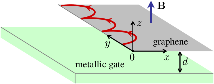
Figure 1: Trajectories of negatively charged electrons deflected by magnetic field $\mathbf{B}$ and bouncing off the graphene edge, which participate in the formation of the magnetoplasmon mode propagating along the $y$ axis. The nearby metallic gate at the distance $d$ is shown at the bottom.

Writing the continuity equation $\partial\rho/\partial t+\mathrm{div}\,\mathbf{j}=0$ for the charge density $\rho=\delta(z)e^{i(\tilde{q}y-\omega t)}\rho(x)$ and the currents $j_{\alpha}=-\sigma_{\alpha\beta}\nabla_{\beta}\varphi$ expressed in terms of the scalar potential $\varphi=e^{i(\tilde{q}y-\omega t)}\varphi(x,z)$, we obtain Volkov ; Wang

$$-i\omega\rho(x)=\Theta(x)\sigma_{xx}(\omega)(\partial_{x}^{2}-\tilde{q}^{2})\varphi(x,0)$$

$$+\delta(x)[\sigma_{xx}(\omega)\partial_{x}+i\tilde{q}\sigma_{xy}(\omega)]\varphi(x,0).$$ (1)

The second equation arises from the three-dimensional Poisson equation $\varepsilon\nabla^{2}\varphi=-4\pi\rho$, where $\varepsilon$ is the dielectric constant of the surrounding medium (we neglect the retardation in the low-frequency limit). Doing a Fourier transform along the $x$ axis and taking into account that $\varphi|_{z=-d}=0$ due to the grounded metallic gate, we can recast it into the integral equation Fetter ; Volkov

$$\varphi(x,0)=\frac{4\pi}{\varepsilon}\int\limits_{0}^{\infty}dx^{\prime}\>L_{\tilde{q},d}(x-x^{\prime})\rho(x^{\prime})$$ (2)

with the kernel

$$L_{\tilde{q},d}(x)=\int\limits_{-\infty}^{+\infty}\frac{dk}{2\pi}\frac{e^{ikx}}{\sqrt{k^{2}+\tilde{q}^{2}}\left[1+\coth(d\sqrt{k^{2}+\tilde{q}^{2}})\right]}.$$ (3)

The system of equations (1)–(3) determines the electromagnetic modes in the system. We can solve it using the Wiener-Hopf method following Ref. Volkov with the only difference that we assume a real frequency $\omega$ and a complex wave vector $\tilde{q}$ instead of complex $\omega$ and real $q$. The final equation for edge magnetoplasmon dispersion is

$$1+\frac{\sigma_{xy}(\omega)}{i\sigma_{xx}(\omega)}\tanh Z(\tilde{q},\omega)=0,$$ (4)

where

$$Z(\tilde{q},\omega)=\frac{1}{2\pi}\int\limits_{-\infty}^{+\infty}\frac{\tilde{q}\>dk}{k^{2}+\tilde{q}^{2}}$$

$$\times\ln\left\{1+\frac{4\pi i\sigma_{xx}(\omega)}{\varepsilon\omega}\frac{\sqrt{k^{2}+\tilde{q}^{2}}}{1+\coth(d\sqrt{k^{2}+\tilde{q}^{2}})}\right\}.$$ (5)

Here $\tilde{q}$ is assumed to have a positive real part, otherwise we need to replace it by $-\tilde{q}$ and change the sigh of the second term in (4). If the dielectric constants above ($\varepsilon_{1}$) and below ($\varepsilon_{2}$) graphene layer are different, then $\varepsilon[1+\coth(d\sqrt{k^{2}+\tilde{q}^{2}})]$ in (5) is replaced by $\varepsilon_{1}+\varepsilon_{2}\coth(d\sqrt{k^{2}+\tilde{q}^{2}})$, which complicates the following calculations Volkov . Nevertheless we can use the approximation of uniform medium with $\varepsilon=(\varepsilon_{1}+\varepsilon_{2})/2$ in the limit $d\rightarrow\infty$ and with $\varepsilon=\varepsilon_{2}$ at $d\rightarrow 0$.

Introducing the dimensionless quantity $\eta=4\pi\tilde{q}\sigma_{xx}(\omega)/i\omega$ Wang , we can find $Z$ as a function of $\eta$ and $\tilde{q}d$. We are interested in the long-wavelength and low-frequency limit, when $\tilde{q},\omega\rightarrow 0$ and $\eta\propto\sigma_{xx}(0)$. In the case of low dissipation we can assume $|\eta|\ll 1$, $\tilde{q}\approx q$, and calculate the analytical asymptotics Volkov of $Z$ in this limit:

$$Z\approx-\frac{\eta}{2\pi}\log\left(-\frac{4e}{\eta}\right), qd\gtrsim e^{-\gamma_{\mathrm{E}}},$$ (6)

$$Z\approx-\frac{\eta}{2\pi}\log\left(-\frac{4e^{1+\gamma_{\mathrm{E}}}qd}{\eta}\right), \displaystyle\frac{|\eta|}{4e^{\gamma_{\mathrm{E}}}}\lesssim qd\lesssim e^{-\gamma_{\mathrm{E}}},$$ (7)

$$Z\approx\sqrt{-\eta qd}, \displaystyle qd\lesssim\frac{|\eta|}{4e^{\gamma_{\mathrm{E}}}},$$ (8)

where $\gamma_{\mathrm{E}}\approx 0.577$ is the Euler gamma constant. Eq. (6) corresponds to the case where the gate is either absent or too far to influence the magnetoplasmons. Eq. (7) corresponds to the opposite limit of local capacitance approximation Johnson , when (2) reduces at small $d$ to the local relationship for the plane capacitor: $\varphi(x)=4\pi d\rho(x)/\varepsilon$. Substituting (6)–(8) to (4), we obtain the dispersion relations for the edge magnetoplasmons Volkov :

$$\omega=-\frac{2q\sigma_{xy}(0)}{\varepsilon}\ln\frac{2e}{qw}, qd\gtrsim e^{-\gamma_{\mathrm{E}}},$$ (9)

$$\omega=-\frac{2q\sigma_{xy}(0)}{\varepsilon}\ln\frac{2e^{1+\gamma_{\mathrm{E}}}d}{w}, \displaystyle\frac{qw}{2e^{\gamma_{\mathrm{E}}}}\lesssim qd\lesssim e^{-\gamma_{\mathrm{E}}},$$ (10)

$$\omega=-\frac{2\pi q\sigma_{xy}(0)}{\varepsilon}\sqrt{\frac{2d}{w}}, \displaystyle qd\lesssim\frac{qw}{2e^{\gamma_{\mathrm{E}}}},$$ (11)

where $w=-(2\pi/\varepsilon)[d\,\mathrm{Im}\,\sigma_{xx}(\omega)/d\omega]|_{\omega=0}$. Since $\sigma_{xy}(0)<0$ at $\mathbf{B}\propto\mathbf{e}_{z}$, we have the edge mode propagating in the positive $y$ direction (Fig. 1). Note that in vanishing magnetic field the dispersion equation (4) reduces to $Z(\tilde{q},\omega)=i\pi/2$ which typically implies $\eta$ of the order of unity ($\eta\approx 2.4344$ at $d\rightarrow\infty$ Volkov ), so the formulas (9)–(11) derived under assumption $|\eta|\ll 1$ become inapplicable.

In the presence of dissipation the expressions (9)–(11) are inaccurate because in the long-wavelength and low-frequency limit probed in the experiments Kumada ; KumadaPRL ; Petkovic ; PetkovicPRL ; KumadaNJP the damping rate dominates the frequency. This should happen even in very clean graphene samples because the magnetoplasmon frequencies are far below the terahertz range. Therefore the real part of $\sigma_{xx}$ dominates the imaginary part connected with $w$ (in other words, the dissipation dominates electron inertial motion). Using (6) and (8) in (4) at $\omega\rightarrow 0$, we obtain the approximations for dispersion law and attenuation rate $\alpha$. At large graphene-to-gate distance $qd\gtrsim 1$ we obtain

$$\omega=\frac{\pi q\sigma_{xx}(0)}{e\varepsilon\,\mathrm{Im}\,Y},\quad\alpha=-q\frac{\mathrm{Re}\,Y}{\mathrm{Im}\,Y},$$ (12)

where $Y$ is the complex solution of the equation $1-iXY\ln Y=0$ with $\mathrm{Re}\,Y<0$, $\mathrm{Im}\,Y>0$, and $X=-2e\sigma_{xy}(0)/\pi\sigma_{xx}(0)$. At very small distances, when $qd\lesssim 0.01$, we obtain

$$\omega=\frac{8\pi q^{2}\sigma_{xy}^{2}(0)d}{\varepsilon\sigma_{xx}(0)},\quad\alpha=q.$$ (13)

Note that, in contrast to the long-wavelength limit of the solution in Ref. Johnson with complex $\omega$ and real $q$, where $\omega$ is purely imaginary, here we have the oscillations highly damped in space with $\tilde{q}=q(1+i)$. At larger distances or wave vectors, when $qd\gtrsim 0.01$, the dispersion becomes linear and attenuation rate decreases.

III Optical conductivity in magnetic field

To calculate the optical conductivity tensor $\sigma_{\alpha\beta}$ in disordered graphene in quantizing magnetic field we use the version of the self-consistent Born approximation Shon which allows us to take into account both formation of Landau levels and their disorder-induced broadening. In this approximation the single-electron Green functions are dressed by interaction with random disorder potential, which results in broadening of each Landau level, and then the current vertex is modified by a disorder ladder. Direct application of the Kubo formula to calculate the current response to the oscillating vector potential $\mathbf{A}=(c/i\omega)\mathbf{E}\propto e^{-i\omega t}$ provides the dynamical conductivity

$$\tilde{\sigma}_{\alpha\beta}(\mathbf{q},\omega)=\frac{ig}{\hbar\omega}G_{j_{\alpha}j_{\beta}}^{\mathrm{R}}(\mathbf{q},\omega)$$ (14)

in terms of the Fourier transform $G_{j_{\alpha}j_{\beta}}^{\mathrm{R}}(\mathbf{q},\omega)=-iS^{-1}\int d\mathbf{r}d\mathbf{r}^{\prime}\int_{0}^{\infty}dt\>e^{-i\mathbf{q}(\mathbf{r}-\mathbf{r}^{\prime})+i\omega t}\langle[j_{\alpha}(\mathbf{r},t),j_{\beta}(\mathbf{r}^{\prime},0)]\rangle$ of the retarded Green function of the current $j_{\alpha}(\mathbf{r},t)=ev_{\mathrm{F}}\psi^{+}(\mathbf{r},t)\sigma_{\alpha}\psi(\mathbf{r},t)$. Here $\psi(\mathbf{r},t)$ is the two-component Heisenberg field operator of massless Dirac electrons in the valley $\mathbf{K}$ of graphene, $v_{\mathrm{F}}\approx 10^{6}\,\mbox{m/s}$ is the Fermi velocity, $g=4$ is the degeneracy over the valleys and spin projections, $S$ is the system area.

However, in practical calculations of (14) the problem of finite limit of $G_{j_{\alpha}j_{\beta}}^{\mathrm{R}}(\mathbf{q},\omega)$ at $\omega\rightarrow 0$ can be encountered (see Gusynin and the example of a clean system considered in Appendix A). As result, $\tilde{\sigma}_{\alpha\beta}$ becomes divergent at low frequencies which we are interested in, which is unphysical for a disordered conductor with nonzero dissipation. At $q=0$, by definition of $G_{j_{\alpha}j_{\beta}}^{\mathrm{R}}$, this divergence corresponds to the unphysical response of the current to static and uniform vector potential, that contradicts the gauge invariance. The same problem of spurious response of graphene to vector potential, arising in calculations of graphene electromagnetic response functions where the momentum cutoff was used to obtain finite results, was reported in Refs. Sabio ; Principi ; Takane . The related problem of spurious Meissner effect, appearing in the non-superconducting state of graphene when the superconducting current of massless Dirac electrons is calculated, was reported Kopnin ; Mizoguchi . To overcome this problem, the unphysical contribution to response functions can be calculated explicitly in the Dirac electron model and then subtracted Principi , the cutoff procedure can be modified Takane , or auxiliary quadratic in momentum terms can be added to Hamiltonian to make its spectrum bounded from below Mizoguchi . Some of these approaches can be modified and applied for electrons in graphene populating Landau levels in a clean system, as shown in Appendix A.

To calculate correct conductivity tensor, which is free from unphysical divergences in the low-frequency limit, we use the $\mathbf{E}\cdot\mathbf{r}$ gauge, which does not involve such unobservable quantities as the vector potential from the very beginning. The use of this gauge is justified in the dipole long-wavelength limit, which is applicable in our case. Indeed, the experiments Kumada ; KumadaPRL ; Petkovic ; PetkovicPRL ; KumadaNJP probe the plasmon wave vectors, $q\ll l_{H}^{-1}$, much smaller than the inverse magnetic length $l_{H}=\sqrt{\hbar c/eB}$, therefore hereafter we consider the limit $q\rightarrow 0$ in conductivity calculations. Using the spectral representation, we show in Appendix B that the optical conductivity in the $\mathbf{E}\cdot\mathbf{r}$ gauge is

$$\sigma_{\alpha\beta}(\omega)=\frac{ig}{\hbar\omega}\left[G_{j_{\alpha}j_{\beta}}^{\mathrm{R}}(\omega)-G_{j_{\alpha}j_{\beta}}^{\mathrm{R}}(\omega=0)\right].$$ (15)

In comparison with (14), here the unphysical response $G_{j_{\alpha}j_{\beta}}^{\mathrm{R}}(\omega=0)$ is subtracted and $\sigma_{\alpha\beta}(\omega)$ is guaranteed to be finite at $\omega\rightarrow 0$. Thus the conductivity calculation in the $\mathbf{E}\cdot\mathbf{r}$ gauge provides physically correct results satisfying the gauge invariance. When Landau level widths are negligible, this approach reduces to those used in Principi ; Takane , as shown by explicit calculations of $G_{j_{\alpha}j_{\beta}}^{\mathrm{R}}(\omega=0)$ in Appendix A. Note that the subtraction similar to those in (15) arises in the case of massive electrons due to the diamagnetic contribution to conductivity Rammer .

The self-consistent Born approximation provides the following expression for the Green function of currents (see also Shon ; Ando ):

$$G_{j_{\alpha}j_{\beta}}^{\mathrm{R}}(\omega)=-\frac{e^{2}v_{\mathrm{F}}^{2}}{2\pi^{2}l_{H}^{2}}\sum_{n_{1}n_{2}}\int\limits_{-\infty}^{+\infty}\frac{F_{\alpha\beta}^{n_{1}n_{2}}\>dz}{1-\gamma_{n_{1}n_{2}}G_{n_{1}}G_{n_{2}}^{*}}$$

$$\times\left\{\frac{n_{\mathrm{F}}(z)G_{n_{1}}\,\mathrm{Im}\,G_{n_{2}}}{1-\gamma_{n_{1}n_{2}}G_{n_{1}}G_{n_{2}}}+\frac{n_{\mathrm{F}}(z+\omega)\,\mathrm{Im}G_{n_{1}}\,G_{n_{2}}^{*}}{1-\gamma_{n_{1}n_{2}}G_{n_{1}}^{*}G_{n_{2}}^{*}}\right\},$$ (16)

where $G_{n_{1}}\equiv G_{n_{1}}^{\mathrm{R}}(z+\omega)$ and $G_{n_{2}}\equiv G_{n_{2}}^{\mathrm{R}}(z)$ are the retarded Green functions of electrons on Landau levels with the numbers $n_{1},n_{2}=0,\pm 1,\pm 2,\ldots$, $n_{\mathrm{F}}(z)=[e^{(\hbar z-\mu)/T}+1]^{-1}$ is the Fermi-Dirac distribution, $\gamma_{n_{1}n_{2}}=(2\pi l_{H}^{2}/\hbar^{2}S)\sum_{kk^{\prime}}\langle\langle\psi_{n_{1}k^{\prime}}|U|\psi_{n_{1}k}\rangle\langle\psi_{n_{2}k}|U|\psi_{n_{2}k^{\prime}}\rangle\rangle_{U}$ is the matrix element of the disorder potential $U$ averaged over its realizations, which appears in the disorder ladder, $\psi_{nk}$ is the electron state on the $n$th Landau level with the $k$th guiding center index. The factor $F_{\alpha\beta}^{n_{1}n_{2}}=2^{\delta_{n_{1}0}+\delta_{n_{2}0}-2}(c_{\alpha}c_{\beta}^{*}\delta_{|n_{1}|-1,|n_{2}|}+c_{\alpha}^{*}c_{\beta}\delta_{|n_{1}|,|n_{2}|-1})$ with $c_{x}=1$, $c_{y}=i$ determines the selection rules $|n_{1}|=|n_{2}|\pm 1$ for the dipole inter-Landau level transitions in graphene.

Eq. (16) takes the simple form in the case of short-range impurities, when $\gamma_{n_{1}n_{2}}$ vanish Shon ; Ando . In this case we can take the electron Green functions $G_{n}^{\mathrm{R}}(\omega)=\int d\omega^{\prime}\>\rho_{n}(\omega^{\prime})/(\omega-\omega^{\prime}+i\delta)$ corresponding to the Lorentzian spectral density $\rho_{n}(\omega)=(\hbar\Gamma/\pi)/[(\hbar\omega-E_{n})^{2}+\Gamma^{2}]$, instead of half-elliptic densities Shon ; Yang appearing as an artefact of the self-consistent Born approximation. Here $E_{n}=\mathrm{sgn}(n)\hbar v_{\mathrm{F}}\sqrt{2|n|}/l_{H}$ and $\Gamma$ are, respectively, the energy and the width of the $n$th Landau level. We assume equal widths of all Landau levels, in agreement with the scanning tunneling spectroscopy experiments (see, e.g., Miller ). From (15)–(16) we obtain the final expression for the conductivity, which behaves correctly in the $\omega\rightarrow 0$ limit:

$$\sigma_{\alpha\beta}(\omega)=\frac{ige^{2}v_{\mathrm{F}}^{2}}{2\pi\hbar l_{H}^{2}}\sum_{n_{1}n_{2}}F_{\alpha\beta}^{n_{1}n_{2}}\int dz_{1}dz_{2}\>\rho_{n_{1}}(z_{1})\rho_{n_{2}}(z_{2})$$

$$\times\frac{n_{\mathrm{F}}(z_{2})-n_{\mathrm{F}}(z_{1})}{(z_{1}-z_{2})(\omega+z_{2}-z_{1}+i\delta)}.$$ (17)

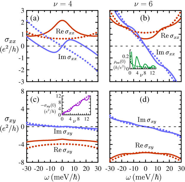
Figure 2: Solid lines: real and imaginary parts of $\sigma_{xx}$ (a,b) and $\sigma_{xy}$ (c,d) as functions of $\omega$ calculated when the Fermi level is located in the center of the 1st Landau level, $\nu=4$ (a,c), or between the 1st and 2nd levels, $\nu=6$ (b,d). Calculations are conducted at $B=12\,\mbox{T}$, $\Gamma=5\,\mbox{meV}$. Dotted lines: Drude conductivities calculated at the same carrier density in the same magnetic field with $\gamma=2\Gamma/\hbar$. Insets in (b) and (c) show the filling-factor dependencies of, respectively, static resistivity $\rho_{xx}(0)$ and Hall conductivity $\sigma_{xy}(0)$ (solid lines) and their Drude counterparts (dotted lines).

The integrals in (17) can be calculated analytically in the limit $T\rightarrow 0$, $n_{\mathrm{F}}(z)\rightarrow\Theta(\mu-\hbar z)$, corresponding to the experiments Kumada ; KumadaPRL ; Petkovic ; PetkovicPRL ; KumadaNJP carried out at cryogenic temperatures. The chemical potential $\mu$ can be connected with the Landau level filling factor: $\nu=g\sum_{n}[\frac{1}{2}\mathrm{sgn}(n)+\int dz\>n_{\mathrm{F}}(z)\rho_{n}(z)]$; $\nu$ is zero for undoped graphene, where the 0th Landau level is half-filled, and increases by 4 for each fully filled Landau level because of the fourfold degeneracy of electron states, so it equals $4n+2$ when the $n$th level is completely filled and $4n$ when the $n$th level is half-filled. We do not take into account the Zeeman splitting of Landau levels or possible symmetry breaking scenarios at fractional fillings because they manifest themselves at much higher magnetic fields.

In the limit of high doping or low magnetic field, when the chemical potential $\mu$ is located between $E_{n}$ and $E_{n+1}$, a single intraband transition $n\rightarrow n+1$ provides a major contribution to (17) Wang ; Witowski . In the limit $n\gg 1$ it takes the form of the classical Drude conductivity in magnetic field

$$\sigma_{xx}(\omega)=\frac{n_{\mathrm{c}}e^{2}}{m^{*}}\frac{i(\omega+i\gamma)}{(\omega+i\gamma)^{2}-\omega_{\mathrm{c}}^{2}},$$ (18)

$$\sigma_{xy}(\omega)=\frac{n_{\mathrm{c}}e^{2}}{m^{*}}\frac{\omega_{\mathrm{c}}}{(\omega+i\gamma)^{2}-\omega_{\mathrm{c}}^{2}},$$ (19)

where $n_{\mathrm{c}}=\nu/2\pi l_{H}^{2}$ is the two-dimensional carrier density, $m^{*}=|\mu|/v_{\mathrm{F}}^{2}$ and $\omega_{\mathrm{c}}=eB/m^{*}c$ are, respectively, the cyclotron mass and frequency, and $\gamma=2\Gamma/\hbar$ is the decay rate of an electron-hole pair.

Examples of $\sigma_{\alpha\beta}(\omega)$ calculated from (17) and in the Drude model (18)–(19) at the same carrier density are shown in Fig. 2. When the Fermi level is located between Landau levels [Fig. 2(b,d)], the conductivity behavior at low frequencies is close to the Drude model predictions, especially at high filling factors. At non-integer filling of Landau levels [Fig. 2(a,c)], the conductivity deviates from the Drude model. Note the marked increase of $\sigma_{xx}$ at low frequencies $|\omega|\lesssim\Gamma$ indicating the dissipation due to intralevel transitions. The second important difference is the positive derivative $d\,\mathrm{Im}\,\sigma_{xx}(\omega)/d\omega|_{\omega=0}>0$ at the half-integer filling in Fig. 2(a), which is indicative of effectively free electrons moving within the Landau level at $|\omega|\lesssim\Gamma$. The similar behavior is demonstrated by a low-frequency Drude conductivity of a typical conductor in the absence of magnetic field: $\mathrm{Im}\,\sigma(\omega)\propto\omega/(\omega^{2}+\gamma^{2})\propto\omega$ at $\omega\rightarrow 0$. In contrast, at the integer filling we see the negative derivative $d\,\mathrm{Im}\,\sigma_{xx}(\omega)/d\omega|_{\omega=0}<0$ in Fig. 2(c), which is typical to bound electrons. This derivative is related to the quantity $w$ in (9)–(11), which can be interpreted Volkov as a distance where the energy of two-dimensional plasma oscillations is comparable with the cyclotron energy. At half-integer fillings, when the dissipation is significant, this quantity has no such meaning, and the formulas (9)–(11) are inapplicable as well. Note the Drude conductivity (18) always demonstrates the insulating behavior $d\,\mathrm{Im}\,\sigma_{xx}(\omega)/d\omega|_{\omega=0}<0$ and thus cannot describe the transitions between conducting and insulating regimes as $\nu$ is changed.

It is instructive to compare (17) with the conductivity, which is initially calculated for a clean graphene in magnetic field, and then supplemented with the phenomenological relaxation rate $2\Gamma/\hbar$ Gusynin :

$$\tilde{\tilde{\sigma}}_{\alpha\beta}(\omega)=\frac{ige^{2}\hbar v_{\mathrm{F}}^{2}}{2\pi l_{H}^{2}}\sum_{n_{1}n_{2}}F_{\alpha\beta}^{n_{1}n_{2}}$$

$$\times\frac{f_{n_{2}}-f_{n_{1}}}{(E_{n_{1}}-E_{n_{2}})(\hbar\omega+E_{n_{2}}-E_{n_{1}}+2i\Gamma)},$$ (20)

where $f_{n}=n_{\mathrm{F}}(E_{n}/\hbar)$. Despite the similarity between (17) and (20), the latter does not take into account electron transitions within the broadened Landau level, which are responsible for the metallic-like behavior [Fig. 2(a)] of $\sigma_{\alpha\beta}(\omega)$ at non-integer Landau level fillings. At low frequencies (20) is numerically very close to the Drude conductivity (18)–(19). Thus the phenomenological relaxation model, similarly to the Drude one, cannot describe the sequence of insulating and conducting regimes.

Although our conductivity demonstrates the qualitatively correct low-frequency properties and properly takes into account the Landau level quantization, further improvement is needed to achieve quantitative agreement with the experiment. For example, the peaks in the static $\rho_{xx}(0)$ [see inset in Fig. 2(b)] and the simultaneously occurring rising parts in the dependence of $\sigma_{xy}(0)$ on $\nu$ between the quantized plateaus [inset in Fig. 2(c)] characteristic to conducting states at non-integer Landau level fillings are broader than in the typical quantum Hall effect measurements Novoselov ; Kumada . From the other side, the broadening of these peaks at nonzero frequencies studied in semiconductor quantum wells Engel ; Saeed should also been taken into account. The conductivity model which explicitly includes consideration of localized and extended states would provide more accurate results in the low-frequency region.

IV Calculation results

Using the formulas (4), (5), (17), we can calculate numerically the dispersion relations $\omega(q)$ and attenuation rates $\alpha(q)$ at different filling factors $\nu$ and graphene-to-gate distances $d$ to study the effects of gate screening and dissipation. We take the parameters $B=12\,\mbox{T}$, $\Gamma=5\,\mbox{meV}$, $\varepsilon=4$, which are close to the experimental conditions Kumada ; KumadaPRL ; Petkovic ; PetkovicPRL ; KumadaNJP where Landau quantization is well developed.

In Fig. 3 we show typical examples of $\omega(q)$ and $\alpha(q)$ calculated in the absence of the gate screening, at $d=\infty$, with the full Landau-level based conductivities (17) and within the Drude model (18)–(19) at the same carrier density. At integer Landau level fillings [$\nu=6$, Fig. 3(b,d)] $\omega$ and $\alpha$ are, respectively, slightly higher and significantly lower than in the Drude model. This indicates that the dissipation, which suppresses $\omega$ and increases $\alpha$, is lower than in the Drude model due to the inter-Landau level gap. At half-integer Landau level fillings [$\nu=4$, Fig. 3(a,c)] the situation is opposite: the dissipation caused by the intralevel transitions slightly suppresses $\omega$ and significantly increases $\alpha$ in comparison with the Drude model. Note also the pronounced dissipation-induced decrease of $\omega$ and increase of $\alpha$ at $\nu=4$ in comparison with $\nu=6$. The numerical calculations in both models are close to the analytical approximation (12) where the corresponding conductivities at $\omega=0$ are substituted. For comparison we plotted the magnetoplasmon frequency calculated with the Drude conductivity of a clean ($\gamma=0$) system, which is higher than in the disordered system and agrees with the analytical approximation (9) very well.

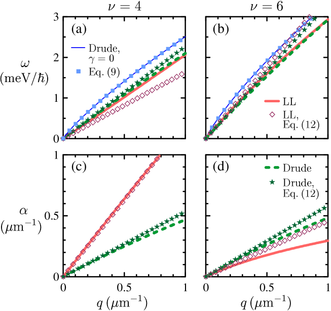
Figure 3: Edge magnetoplasmon frequencies $\omega$ (a,b) and attenuation rates $\alpha$ (c,d) as functions of the wave vector $q$ calculated in the absence of gate screening at $d=\infty$, at half-integer [$\nu=4$, (a,c)] and integer [$\nu=6$, (b,d)] Landau level fillings at $B=12\,\mbox{T}$, $\Gamma=5\,\mbox{meV}$, $\varepsilon=4$. The curves show numerical calculation results with Landau-level based (LL) and Drude conductivities, and with Drude conductivity in a clean ($\gamma=0$) system. The analytical approximations are shown by the points.

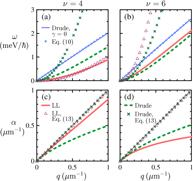
Figure 4: The same as in Fig. 3 but in the presence of the gate screening at $d=200\,\mbox{nm}$.

The similar calculation results in the presence of the screening gate at $d=200\,\mbox{nm}$ are shown in Fig. 4. We see the overall suppression of $\omega$ in comparison with the ungated case, which becomes even stronger in the presence of dissipation. At integer [$\nu=6$, Fig. 4(b,d)] and half-integer [$\nu=4$, Fig. 4(a,c)] Landau level fillings we again see the effect of, respectively, decreased and enhanced dissipation on $\omega$ and $\alpha$. The analytical approximation (13) predicting highly damped mode with quadratic dispersion at small $d$ is applicable only at very low distances or wave vectors, $qd\lesssim 0.01$, while at higher $q$ the dispersion laws become linear. Calculations with the Drude conductivity of a clean system agree with (11) and provide considerably higher $\omega$.

In Fig. 5 we show the edge magnetoplasmon phase velocity $v=\omega/q$ and quality factor $Q=q/2\alpha$ calculated at $q=0.2\,\mu\mbox{m}^{-1}$ (where dispersions are almost linear) as functions of the filling factor $\nu$ both in the absence and in the presence of the metallic gate. As expected from the aforementioned dissipation-induced frequency suppression, we observe the dips in both $v$ and $Q$ when the Fermi level is located in the centers of Landau levels ($\nu=4,8,12,16$). In Fig. 5(a) these dips are slightly displaced to the left, perhaps, due to the general rising trend of $v(\nu)$, and also demonstrate some extra oscillations, which can be an artefact of the model used to calculate the conductivity. On the contrary, when the Fermi level is located in the middle of any inter-Landau level gap ($\nu=2,6,10,14$), $v$ and $Q$ have peaks due to reduced dissipation. The oscillations of $v(\nu)$ and $Q(\nu)$ occur around the smooth results of the quasiclassical Drude model, which is insensitive to how the individual Landau levels are filled. Comparison with the calculations for a clean system shows that the gate screening not only reduces the velocity, but also enhances the dissipation-induced suppression of $v$ and $Q$. As in the previous picture, the analytical formula (12) well describes the dispersion and damping at $d=\infty$, while the formula (13) for small $d$ is applicable only in the regions of low velocity and high dissipation.

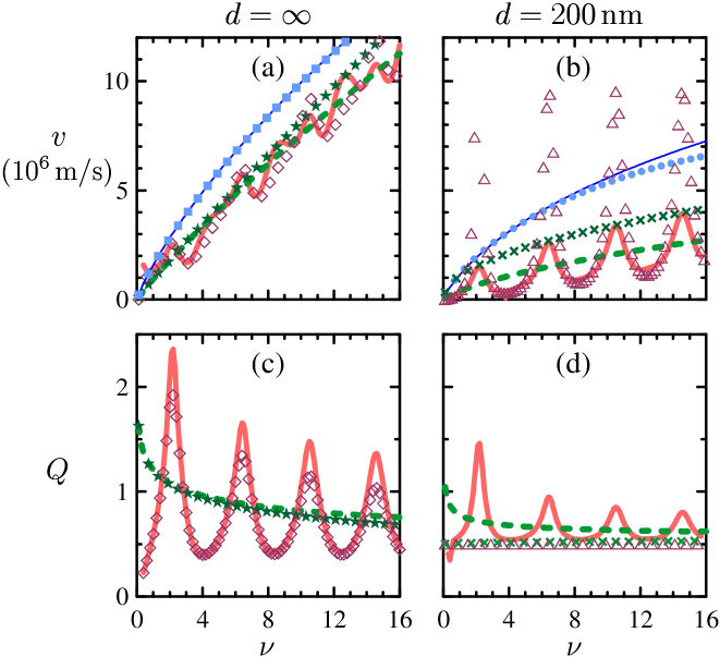
Figure 5: Edge magnetoplasmon velocities $v$ (a,b) and quality factors $Q$ (c,d) as functions of the Landau level filling factor $\nu$ at $q=0.2\,\mu\mbox{m}^{-1}$ in the absence [$d=\infty$, (a,c)] and in the presence [$d=200\,\mbox{nm}$, (b,d)] of the gate screening at $B=12\,\mbox{T}$, $\Gamma=5\,\mbox{meV}$, $\varepsilon=4$. The curves show numerical calculation results with Landau-level based (LL) and Drude conductivities, and with Drude conductivity in a clean system, and the points show analytical approximations. The notations for curves and points on the panels (a,c) and (b,d) are the same as in, respectively, Figs. 3 and 4.

V Conclusions

We considered the magnetoplasmon modes propagating along graphene edge in quantizing magnetic fields in the presence of the grounded metallic gate. The relationship between real frequencies and complex wave vectors (with the imaginary part responsible for the damping) of these modes was obtained using the Wiener-Hopf method in a form of algebraic equation (4)–(5). The optical conductivity tensor $\sigma_{\alpha\beta}(\omega)$ was calculated at low temperatures using the self-consistent Born approximation for graphene in magnetic field in the limit of short-range impurities and with the assumption of Lorentzian broadening of Landau levels. The use of the $\mathbf{E}\cdot\mathbf{r}$ gauge turned out to be convenient to calculate the conductivity which behaves correctly at low frequencies. The quasiclassical Drude approximation to the conductivity, valid in the limit of large number of filled Landau level, was also considered for comparison. The magnetoplasmon dispersions, attenuation rates, velocities and quality factors were calculated both in the absence and in the presence of the gate at different Landau level filling factors.

The analysis of the calculation results allows us to make the following conclusions:

(a) At integer filling of Landau levels ($\nu=2,6,10,\ldots$), where the Fermi level is located in the interlevel gap, the dissipation is low, and the frequency, velocity and life time of the edge magnetoplasmon are increased in comparison to the predictions of the Drude model. On the contrary, at half-integer filling of Landau levels ($\nu=4,8,12,\ldots$), where the Fermi level lies within a broadened Landau level, the dissipation is enhanced due to intralevel transitions, and the frequency, velocity and life time of the edge magnetoplasmon are suppressed. So our approach predicts the oscillations of the edge magnetoplasmon velocity when the filling factor is changed, which are superimposed on the smooth trend of growing velocity as the carrier density increases. The commonly used Wang ; Witowski Drude conductivity model describes only the latter because it does not take into account Landau level quantization.

(b) The electric field screening caused by a nearby metallic gate decreases the frequency and velocity of the mode, and makes their dissipation-induced suppression at non-integer filling of Landau levels much more pronounced.

(c) The analytical formulas (9)–(11) for the mode frequency, which are frequently used to analyze the experimental data Kumada ; KumadaPRL ; Petkovic ; PetkovicPRL ; KumadaNJP , are applicable only for very clean systems. The quantity $w$ entering these formulas lose its meaning at half-integer Landau level fillings, when the dissipation is significant. Eq. (12) can be used instead in the case when the gate screening is negligible. The important feature of the experimental conditions is that plasmons are probed at relatively low frequencies not exceeding the terahertz range, so any realistic rate of dissipation due to inter-Landau level transitions dominates the frequency and substantially modifies mode properties in comparison with the predictions for a clean system.

Our conclusions are in qualitative agreement with the experimental data Kumada ; KumadaPRL ; Petkovic ; PetkovicPRL ; KumadaNJP , where the suppression of the magnetoplasmon velocities at non-integer Landau level fillings was observed. Our approach assume the abrupt edge of graphene and does not take into account the details of spatial structure of Landau level wave functions near the edge, which include formation of incompressible stripes Johnson , edge channels Petkovic ; Balev ; Andreev , and electron drift due to electric field normal to the edge PetkovicPRL ; KumadaPRL . Analysis of these details requires an essential complication of our approach and is beyond the scope of this paper.

To study the effects of Landau level filling on the edge magnetoplasmon we used the model for the optical conductivity providing qualitatively correct description of its low-frequency behavior and the filling-factor dependence. A refined model, which takes into account the localized states and their scaling properties, can provide an additional insight into the theory of edge magnetoplasmons in quantum Hall regime and bring the results of our approach into better quantitative agreement with the experiments.

Appendix A Cutoff treatment in magnetic field

In the clean limit the single-electron spectral densities are $\rho_{n}(\omega)=\delta(\omega-E_{n}/\hbar)$ and the Green function of currents (16) at $\omega\rightarrow 0$ takes the form (notations are taken from Sec. III and the limit $q\rightarrow 0$ is implied)

$$G_{j_{\alpha}j_{\beta}}^{\mathrm{R}}(0)=\frac{e^{2}\hbar v_{\mathrm{F}}^{2}}{2\pi l_{H}^{2}}\sum_{n_{1}n_{2}}F_{\alpha\beta}^{n_{1}n_{2}}\frac{f_{n_{2}}-f_{n_{1}}}{E_{n_{2}}-E_{n_{1}}}.$$ (21)

Imposing the usual cutoff for Landau level summation $-N\leqslant n_{1},n_{2}\leqslant N$ and taking into account explicit forms of $F_{\alpha\beta}^{n_{1}n_{2}}$ and $E_{n}$, we obtain after some algebra

$$G_{j_{\alpha}j_{\beta}}^{\mathrm{R}}(0)=\frac{\delta_{\alpha\beta}e^{2}v_{\mathrm{F}}}{2\sqrt{2}\pi l_{H}}$$

$$\times\sum_{n=0}^{N-1}\left[\sqrt{n+1}(f_{n+1}-f_{-n-1})-\sqrt{n}(f_{n}-f_{-n})\right].$$ (22)

Note that if even one of Landau level numbers $n_{1}$ or $n_{2}$ exceeds the cutoff then the whole transition $n_{2}\rightarrow n_{1}$ is dropped out of the sum (21). Since the cutoff energy $E_{N}$ should be much larger than the temperature, we can assume $f_{N}=0$, $f_{-N}=1$, so after cancelation of the most of terms in (22) we have

$$G_{j_{\alpha}j_{\beta}}^{\mathrm{R}}(0)=-\frac{\delta_{\alpha\beta}e^{2}v_{\mathrm{F}}}{2\sqrt{2}\pi l_{H}}\sqrt{N}=-\frac{\delta_{\alpha\beta}e^{2}E_{N}}{4\pi\hbar}.$$ (23)

Thus, in agreement with Sabio ; Principi ; Takane , we obtain the unphysical response of graphene to static and uniform vector potential proportional to the cutoff energy.

To overcome this problem, we can change the cutoff procedure by extending the summation over $n_{1},n_{2}$ in (21) to infinity and transferring the cutoff into the occupation numbers by assuming $f_{n}=n_{\mathrm{F}}(E_{n}/\hbar)\Theta(E_{N}-|E_{n}|)$ [with $\Theta(0)=1$]. The similar procedure for free electrons in the absence of magnetic field was proposed in Takane . Now if one of Landau level numbers in the transition $n_{2}\rightarrow n_{1}$ exceeds the cutoff then the corresponding level is treated as unoccupied one, and the whole transition is not dropped out of the sum. The resulting response function with the modified cutoff procedure

$$G_{j_{\alpha}j_{\beta}}^{\mathrm{R}}(0)=\frac{\delta_{\alpha\beta}e^{2}v_{\mathrm{F}}}{2\sqrt{2}\pi l_{H}}\left\{\sum_{n=0}^{N-1}\sqrt{n+1}(f_{n+1}-f_{-n-1})\right.$$

$$\left.-\sum_{n=0}^{N}\sqrt{n}(f_{n}-f_{-n})\right\}=0$$ (24)

vanishes in contrast to (22) due to different summation limits. However it is hard to apply this procedure in a general case where interactions or disorder are present.

Appendix B Conductivity in the $\mathbf{E}\cdot\mathbf{r}$ gauge

Calculating the conductivity as a response of the current $j_{\alpha}\equiv j_{\alpha}(\mathbf{q}=0)$ to the perturbation of the Hamiltonian $-er_{\beta}E_{\beta}$ using the Kubo formula Giuliani , we get

$$\sigma_{\alpha\beta}(\omega)=\frac{ieg}{\hbar S}\int\limits_{0}^{\infty}dt\>e^{i(\omega+i\delta)t}\left\langle[j_{\alpha}(t),r_{\beta}]\right\rangle.$$ (25)

Assuming existence of a complete set of many-body states $|n\rangle$ of the system with the energies $\tilde{E}_{n}$ and occupation probabilities $p_{n}$, we find the spectral representation Giuliani of (25):

$$\sigma_{\alpha\beta}(\omega)=-\frac{eg}{\hbar S}\sum_{nk}(p_{n}-p_{k})\frac{\langle n|j_{\alpha}|k\rangle\langle k|r_{\beta}|n\rangle}{\omega-\omega_{kn}+i\delta},$$ (26)

where $\omega_{kn}=(\tilde{E}_{k}-\tilde{E}_{n})/\hbar$. Using the commutation relation $[H,r_{\alpha}]=-i\hbar v_{\mathrm{F}}\sigma_{\alpha}$ we obtain the relationship $\langle k|r_{\beta}|n\rangle=\langle k|j_{\beta}|n\rangle/ie\omega_{kn}$, which allows to rewrite (26) as

$$\sigma_{\alpha\beta}(\omega)=\frac{ig}{\hbar S}\sum_{nk}(p_{n}-p_{k})\frac{\langle n|j_{\alpha}|k\rangle\langle k|j_{\beta}|n\rangle}{\omega_{kn}(\omega-\omega_{kn}+i\delta)}.$$ (27)

On the other hand, we can write the spectral representation for the Green function of currents:

$$G_{j_{\alpha}j_{\beta}}^{\mathrm{R}}(\omega)=\frac{1}{S}\sum_{nk}(p_{n}-p_{k})\frac{\langle n|j_{\alpha}|k\rangle\langle k|j_{\beta}|n\rangle}{\omega-\omega_{kn}+i\delta}.$$ (28)

Using the simple equality

$$\frac{1}{\omega-\omega_{kn}+i\delta}+\frac{1}{\omega_{kn}}=\frac{\omega}{\omega_{kn}(\omega-\omega_{kn}+i\delta)},$$ (29)

we finally obtain (15). Note that the subtraction of $G_{j_{\alpha}j_{\beta}}^{\mathrm{R}}(0)$, which distinguishes (15) from (14), turns out to be equivalent to replacement of $\omega$ in the denominator to the frequency $\omega_{kn}$ of each individual transition in the sum. Sometimes this replacement is made manually in approximate conductivity calculations in order to obtain physically reasonable results (see, e.g., Gusynin ).

The anomalous character of the nonzero $G_{j_{\alpha}j_{\beta}}^{\mathrm{R}}(0)$ can be revealed by taking $\omega=0$ in (28) and using again the relationship $\langle k|j_{\beta}|n\rangle=ie\omega_{kn}\langle k|r_{\beta}|n\rangle$:

$$G_{j_{\alpha}j_{\beta}}^{\mathrm{R}}(0)=\frac{ie}{S}\sum_{nk}p_{n}\left[\langle n|j_{\alpha}|k\rangle\langle k|r_{\beta}|n\rangle\right.$$

$$\left.-\langle n|r_{\beta}|k\rangle\langle k|j_{\alpha}|n\rangle\right].$$ (30)

If the summation over the states is made over complete basis, we can use the completeness condition $\sum_{k}|k\rangle\langle k|=I$ and obtain $G_{j_{\alpha}j_{\beta}}^{\mathrm{R}}(0)=(ie/S)\langle[j_{\alpha},r_{\beta}]\rangle=0$. However the cutoff imposed in practical calculations prevents this cancelation as noted in Sabio and illustrated in Appendix A.

References

- (1) A. Politano and G. Chiarello, Plasmon modes in graphene: status and prospect, Nanoscale 6, 10927 (2014).
- (2) S. Xiao, X. Zhu, B.-H. Li, N. A. Mortensen, Graphene-plasmon polaritons: From fundamental properties to potential applications, Front. Phys. 11, 117801 (2016).
- (3) P. A. D. Gonçalves and N. M. R. Peres, An Introduction to Graphene Plasmonics (World Scientific, Singapore, 2016).
- (4) I. Crassee, M. Orlita, M. Potemski, A. L. Walter, M. Ostler, Th. Seyller, I. Gaponenko, J. Chen, and A. B. Kuzmenko, Intrinsic Terahertz Plasmons and Magnetoplasmons in Large Scale Monolayer Graphene, Nano Lett. 12, 2470 (2012).
- (5) H. Yan, Z. Li, X. Li, W. Zhu, P. Avouris, and F. Xia, Infrared Spectroscopy of Tunable Dirac Terahertz Magneto-Plasmons in Graphene, Nano Lett. 12, 3766 (2012).
- (6) A. M. Witowski, M. Orlita, R. Stȩpniewski, A. Wysmołek, J. M. Baranowski, W. Strupiński, C. Faugeras, G. Martinez, and M. Potemski, Quasiclassical cyclotron resonance of Dirac fermions in highly doped graphene, Phys. Rev. B 82, 165305 (2010).
- (7) M. Orlita, I. Crassee, C. Faugeras, A. B. Kuzmenko, F. Fromm, M. Ostler, Th. Seyller, G. Martinez, M. Polini, and M. Potemski, Classical to quantum crossover of the cyclotron resonance in graphene: a study of the strength of intraband absorption, New J. Phys. 14, 095008 (2012).
- (8) N. Kumada, H. Kamata, and T. Fujisawa, Edge magnetoplasmon transport in gated and ungated quantum Hall systems, Phys. Rev. B 84, 045314 (2011).
- (9) I. V. Andreev, V. M. Muravev, D. V. Smetnev, and I. V. Kukushkin, Acoustic magnetoplasmons in a two-dimensional electron system with a smooth edge, Phys. Rev. B 86, 125315 (2012).
- (10) M. Hashisaka, H. Kamata, N. Kumada, K. Washio, R. Murata, K. Muraki, and T. Fujisawa, Distributed-element circuit model of edge magnetoplasmon transport, Phys. Rev. B 88, 235409 (2013).
- (11) N. Kumada, S. Tanabe, H. Hibino, H. Kamata, M. Hashisaka, K. Muraki, and T. Fujisawa, Plasmon transport in graphene investigated by time-resolved electrical measurements, Nat. Commun. 4, 1363 (2012).
- (12) N. Kumada, P. Roulleau, B. Roche, M. Hashisaka, H. Hibino, I. Petković, and D. C. Glattli, Resonant Edge Magnetoplasmons and Their Decay in Graphene, Phys. Rev. Lett. 113, 266601 (2014).
- (13) I. Petković, F. I. B. Williams, K. Bennaceur, F. Portier, P. Roche, and D. C. Glattli, Carrier Drift Velocity and Edge Magnetoplasmons in Graphene, Phys. Rev. Lett. 110, 016801 (2013).
- (14) I. Petković, F. I. B. Williams, and D. C. Glattli, Edge magnetoplasmons in graphene, J. Phys. D: Appl. Phys. 47, 094010 (2014).
- (15) N. Kumada, R. Dubourget, K. Sasaki, S. Tanabe, H. Hibino, H. Kamata, M. Hashisaka, K. Muraki, and T. Fujisawa, Plasmon transport and its guiding in graphene, New J. Phys. 16, 063055 (2014).
- (16) A. L. Fetter, Edge magnetoplasmons in a bounded two-dimensional electron fluid, Phys. Rev. B 32, 7676 (1985).
- (17) V. A. Volkov and S. A. Mikhailov, Edge magnetoplasmons: low frequency weakly damped excitations in inhomogeneous two-dimensional electron systems, Sov. Phys. JETP 67, 1639 (1988).
- (18) W. Wang, J. M. Kinaret, and S. P. Apell, Excitation of edge magnetoplasmons in semi-infinite graphene sheets: Temperature effects, Phys. Rev. B 85, 235444 (2012).
- (19) M. D. Johnson, G. Vignale, Dynamics of dissipative quantum Hall edges, Phys. Rev. B 67, 205332 (2003).
- (20) N. H. Shon and T. Ando, Quantum Transport in Two-Dimensional Graphite System, J. Phys. Soc. Jpn. 67, 2421 (1998).
- (21) V. P. Gusynin, S. G. Sharapov, and J. P. Carbotte, Magneto-optical conductivity in graphene, J. Phys.: Condens. Matter 19, 026222 (2007).
- (22) J. Sabio, J. Nilsson, and A. H. Castro Neto, f-sum rule and unconventional spectral weight transfer in graphene, Phys. Rev. B 78, 075410 (2008).
- (23) A. Principi, M. Polini, and G. Vignale, Linear response of doped graphene sheets to vector potentials, Phys. Rev. B 80, 075418 (2009).
- (24) Y. Takane, Gauge-Invariant Cutoff for Dirac Electron Systems with a Vector Potential, J. Phys. Soc. Jpn. 88, 034702 (2019).
- (25) N. B. Kopnin and E. B. Sonin, Supercurrent in superconducting graphene, Phys. Rev. B 82, 014516 (2010).
- (26) T. Mizoguchi and M. Ogata, Meissner Effect of Dirac Electrons in Superconducting State Due to Inter-Band Effect, J. Phys. Soc. Jpn. 84, 084704 (2015).
- (27) J. Rammer, Quantum Transport Theory (Perseus Books, Reading, 1998).
- (28) T. Ando, Theory of Cyclotron Resonance Lineshape in a Two-Dimensional Electron System, J. Phys. Soc. Jpn. 38, 989 (1975).
- (29) C. H. Yang, F. M. Peeters, and W. Xu, Landau-level broadening due to electron-impurity interaction in graphene in strong magnetic fields, Phys. Rev. B 82, 075401 (2010).
- (30) D. L. Miller, K. D. Kubista, G. M. Rutter, M. Ruan, W. A. de Heer, P. N. First, and J. A. Stroscio, Observing the quantization of zero mass carriers in graphene, Science 324, 924 (2009).
- (31) K. S. Novoselov, A. K. Geim, S. V. Morozov, D. Jiang, M. I. Katsnelson, I. V. Grigorieva, S. V. Dubonos, and A. A. Firsov, Two-dimensional gas of massless Dirac fermions in graphene, Nature 438, 197 (2005).
- (32) L. W. Engel, D. Shahar, Ç. Kurdak, and D. C. Tsui, Microwave Frequency Dependence of Integer Quantum Hall Effect: Evidence for Finite-Frequency Scaling, Phys. Rev. Lett. 71, 2638 (1993).
- (33) K. Saeed, N. A. Dodoo-Amoo, L. H. Li, S. P. Khanna, E. H. Linfield, A. G. Davies, and J. E. Cunningham, Impact of disorder on frequency scaling in the integer quantum Hall effect, Phys. Rev. B 84, 155324 (2011).
- (34) O. G. Balev, P. Vasilopoulos, and H. O. Frota, Edge magnetoplasmons in wide armchair graphene ribbons, Phys. Rev. B 84, 245406 (2011).
- (35) G. F. Giuliani and G. Vignale, Quantum Theory Of The Electron Liquid (Cambridge Univ. Press, Cambridge, 2005).