Analysis of Global Fixed-Priority Scheduling for Generalized Sporadic DAG Tasks

Abstract.

We consider global fixed-priority (G-FP) scheduling of parallel tasks, in which each task is represented as a directed acyclic graph (DAG). We summarize and highlight limitations of the state-of-the-art analyses for G-FP and propose a novel technique for bounding interfering workload, which can be applied directly to generalized DAG tasks. Our technique works by constructing optimization problems for which the optimal solution values serve as safe and tight upper bounds for interfering workloads. Using the proposed workload bounding technique, we derive a response-time analysis and show that it improves upon state-of-the-art analysis techniques for G-FP scheduling.

1. Introduction

With the prevalence of multiprocessor platforms and parallel programming languages and runtime systems such as OpenMP (OpenMP, 2019), Cilk Plus (Frigo et al., 1998; Intel Cilk Plus, 2019), and Intel’s Threading Building Blocks (Intel Threading Building Blocks, 2019), the demand for computer programs to be able to exploit the parallelism offered by modern hardware is inevitable. In recent years, the real-time systems research community has worked to address this trend for real-time applications that require parallel execution to satisfy their deadlines, such as real-time hybrid simulation of structures (Ferry et al., 2014), and autonomous vehicles (Kim et al., 2013).

Much effort has been made to develop analysis techniques and schedulability tests for scheduling parallel real-time tasks under scheduling algorithms such as Global Earliest Deadline First (G-EDF), and Global Deadline Monotonic (G-DM). However, schedulability analysis for parallel tasks is inherently more complex than for conventional sequential tasks. This is because intra-task parallelism is allowed within individual tasks, which enables each individual task to execute simultaneously upon multiple processors. The parallelism of each task can also vary as it is executing, as it depends on the precedence constraints imposed on the task. Consequently, this raises questions of how to account for inter-task interference caused by other tasks on a task and intra-task interference among threads of the task itself.

In this paper, we consider task systems that consist of parallel tasks scheduled under Global Fixed-Priority (G-FP), in which each task is represented by a Directed Acyclic Graph (DAG). Our analysis is based on the concepts of critical interference and critical chain (Chwa et al., 2013; Melani et al., 2015; Chwa et al., 2017), which allow the analysis to focus on a special chain of sequential segments of each task, and hence enable us to use techniques similar to the ones developed for sequential tasks (Baker, 2003; Bertogna et al., 2005; Bertogna and Cirinei, 2007; Bertogna et al., 2009).

The contributions of this paper are as follows:

• We summarize the state-of-the-art analyses for G-FP and highlight their limitations, specifically for the calculation of interference of carry-in jobs and carry-out jobs.

• We propose a new technique for computing upper-bounds on carry-out workloads, by transforming the problem into an optimization problem that can be solved by modern optimization solvers.

• We present a response-time analysis, using the workload bound computed with the new technique. Experimental results for randomly generated DAG tasks confirm that our technique dominates existing analyses for G-FP.

The rest of this paper is organized as follows. In Sections 2 and 3 we discuss related work and present the task model we consider in this paper. Section 4 reviews the concepts of critical interference and critical chain and discusses a general framework to bound response-time. Section 5 summarizes the most recent analyses of G-FP, and also highlights limitations of those analyses. In Section 6 we propose a new technique to bound carry-out workload. A response-time analysis and a discussion of the complexity of our method are given in Section 7. Section 8 presents the evaluation of our method for randomly generated DAG tasks. We conclude our work in Section 9.

2. Related Work

For the sequential task model, Bertogna et al. (Bertogna and Cirinei, 2007) proposed a response-time analysis that works for G-EDF and G-FP. They bound the interference of a task in a problem window by the worst-case workload it can generate in that window. The worst-case workload is then bounded by considering a worst-case release pattern of the interfering task. This technique was later extended by others to analyze parallel tasks, as is done in this work. Bertogna et al. (Bertogna et al., 2009) proposed a sufficient slack-based schedulability test for G-EDF and G-FP in which the slack values for the tasks are used in an iterative algorithm to improve the schedulability gradually. Later, Guan et al. (Guan et al., 2009) proposed a new response-time analysis for both constrained-deadline and arbitrary-deadline tasks.

Initially, simple parallel real-time task models were studied, such as the fork-join task model and the synchronous task model. Lakshmanan et al. (Lakshmanan et al., 2010) presented a transformation algorithm to schedule fork-join tasks where all parallel segments of each task must have the same number of threads, which must be less than the number of processors. They also proved a resource augmentation bound of 3.42 for their algorithm. Saifullah et al. (Saifullah et al., 2013) improved on that work by removing the restriction on the number of threads in parallel segments. They proposed a task decomposition algorithm and proved resource augmentation bounds for the algorithm under G-EDF and Partitioned Deadline Monotonic (P-DM) scheduling. Axer et al. (Axer et al., 2013) presented a response-time analysis for fork-join tasks under Partitioned Fixed-Priority (P-FP) scheduling. Chwa et al. (Chwa et al., 2013) developed an analysis for synchronous parallel tasks scheduled under G-EDF. They introduced the concept of critical interference and presented a sufficient test for G-EDF. Maia et al. (Maia et al., 2014) reused the concept of critical interference to introduce a response-time analysis for synchronous tasks scheduled under G-FP. A general parallel task model was presented by Baruah et al. (Baruah et al., 2012) in which each task is modeled as a Directed Acyclic Graph (DAG) and can have an arbitrary deadline. They presented a polynomial test and a pseudo-polynomial test for a DAG task scheduled with EDF and proved their speedup bounds. However, they only considered a single DAG task. Bonifaci et al. (Bonifaci et al., 2013) later developed feasibility tests for task systems with multiple DAG tasks, scheduled under G-EDF and G-DM.

Melani et al. (Melani et al., 2015) proposed a response-time analysis for conditional DAG tasks where each DAG can have conditional vertices. Their analysis utilizes the concepts of critical interference and critical chain, and works for both G-EDF and G-FP. However, the bounds for carry-in and carry-out workloads are likely to be overestimated since they ignore the internal structures of the tasks. Chwa et al. (Chwa et al., 2017) extended their work in (Chwa et al., 2013) for DAG tasks scheduled under G-EDF. They proposed a sufficient, workload-based schedulability test and improved it by exploiting slack values of the tasks. Fonseca et al. (Fonseca et al., 2017) proposed a response-time analysis for sporadic DAG tasks scheduled under G-FP that improves upon the response-time analysis in (Melani et al., 2015). They improve the upper bounds for interference by taking the DAGs of the tasks into consideration. In particular, by explicitly considering the DAGs the workloads generated by the carry-in and carry-out jobs can be reduced compared to the ones in (Melani et al., 2015), and hence schedulability can be improved. The carry-in workload is bounded by considering a schedule for the carry-in job with unrestricted processors, in which subtasks execute as soon as they are ready and for their full WCETs. The carry-out workload is bounded for a less general type of DAG tasks, called nested fork-join DAGs. We discuss the state-of-the-art analyses for G-FP and differentiate our work in detail in Section 5.

3. System Model

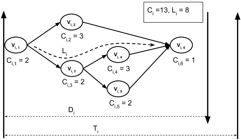
Figure 1. An example DAG task.

We consider a set $\tau$ of $n$ real-time parallel tasks, $\tau=\{\tau_{1},\tau_{2},...,\tau_{n}\}$, scheduled preemptively by a global fixed-priority scheduling algorithm upon $m$ identical processors. Each task $\tau_{i}$ is a recurrent, sporadic process which may release an infinite sequence of jobs and is modeled by $\tau_{i}=\{G_{i},D_{i},T_{i}\}$, where $D_{i}$ denotes its relative deadline and $T_{i}$ denotes the minimum inter-arrival time of two consecutive jobs of $\tau_{i}$. We assume that all tasks have constrained deadlines, i.e., $D_{i}\leq T_{i},\forall i\in[1,n]$. Each task $\tau_{i}$ is represented as a Directed Acyclic Graph (DAG) $G_{i}=(V_{i},E_{i})$, where $V_{i}=\{v_{i,1},v_{i,2},...,v_{i,n_{i}}\}$ is the set of vertices of the DAG $G_{i}$ and $E_{i}\subseteq(V_{i}\times V_{i})$ is the set of directed edges of $G_{i}$. In this paper, we also use subtasks and nodes to refer to the vertices of the tasks. Each subtask $v_{i,a}$ of $G_{i}$ represents a section of instructions that can only be run sequentially. A subtask $v_{i,a}$ is called a predecessor of $v_{i,b}$ if there exists an edge from $v_{i,a}$ to $v_{i,b}$ in $G_{i}$, i.e., $(v_{i,a},v_{i,b})\in G_{i}$. Subtask $v_{i,b}$ is then called a successor of $v_{i,a}$. Each edge $(v_{i,a},v_{i,b})$ represents a precedence constraint between the two subtasks. A subtask is ready if all of its predecessors have finished. Whenever a task releases a job, all of its subtasks are released and have the same deadline as the job’s deadline. We use $J_{i}$ to denote an arbitrary job of $\tau_{i}$ which has release time $r_{i}$ and absolute deadline $d_{i}$.

Each subtask $v_{i,a}$ has a worst-case execution time (WCET), denoted by $C_{i,a}$. The sum of WCETs of all subtasks of $\tau_{i}$ is the worst-case execution time of the whole task, and is denoted by $C_{i}=\sum_{v_{i,a}\in V_{i}}C_{i,a}$. The WCET of a task is also called its work. A sequence of subtasks $(v_{i,u_{1}},v_{i,u_{2}},...,v_{i,u_{t}})$ of $\tau_{i}$, in which $(v_{i,u_{j}},v_{i,u_{j+1}})\in E_{i},\forall 1\leq j\leq t-1$, is called a chain of $\tau_{i}$ and is denoted by $\lambda_{i}$. The length of a chain $\lambda_{i}$ is the sum of the WCETs of subtasks in $\lambda_{i}$ and is denoted by $len(\lambda_{i})$, i.e., $len(\lambda_{i})=\sum_{v_{i,u_{j}}\in\lambda_{i}}C_{i,u_{j}}$. A chain of $\tau_{i}$ which has the longest length is a critical path of the task. The length of a critical path of a DAG is called its critical path length or span, and is denoted by $L_{i}$. Figure 1 illustrates an example DAG task $\tau_{i}$ with 6 subtasks, whose work and span are $C_{i}=13$ and $L_{i}=8$, respectively. In this paper, we consider tasks that are scheduled using a preemptive, global fixed-priority algorithm where each task is assigned a fixed task-level priority. All subtasks of a task have the same priority as the task. Without loss of generality, we assume that tasks have distinct priorities, and $\tau_{i}$ has higher priority than $\tau_{k}$ if $i<k$.

4. Background

In this section we discuss the concept of critical interference that our work is based on, and present a general framework to bound response-times of DAG tasks scheduled under G-FP. In the next section, we summarize the state-of-the-art analyses for G-FP and give an overview of our method.

4.1. Critical Chain and Critical Interference

The notions of critical chain and critical interference were introduced by Chwa et al. (Chwa et al., 2017, 2013) for analyzing parallel tasks scheduled with G-EDF. Unlike sequential tasks, analysis of DAG tasks with internal parallelism is inherently more complicated: (i) some subtasks of a task can be interfered with by other subtasks of the same task (i.e., intra-task interference); (ii) subtasks of a task can be interfered with by subtasks of higher-priority tasks (i.e., inter-task interference); and (iii) the parallelism of a DAG task may vary during execution, subject to the precedence constraints imposed by its graph. The critical chain and critical interference concepts alleviate the complexity of the analysis by focusing on a special chain of subtasks of a task which accounts for its response time, thus bringing the problem closer to a more familiar analysis technique for sequential tasks. Although they were originally proposed for analysis of G-EDF (Chwa et al., 2017, 2013), these concepts are also useful for analyzing G-FP. We therefore use them in our analysis and include a discussion of them in this section.

Consider any job $J_{k}$ of a task $\tau_{k}$ and its corresponding schedule. A last-completing subtask of $J_{k}$ is a subtask that completes last among all subtasks in the schedule of $J_{k}$. A last-completing predecessor of a subtask $v_{k,a}$ is a predecessor that completes last among all predecessors of $v_{k,a}$ in the schedule of $J_{k}$. Note that a subtask can only be ready after a last-completing predecessor finishes, since only then are all the precedence constraints for the subtask satisfied. Starting from a last-completing subtask of $J_{k}$, we can recursively trace back through all last-completing predecessors until we reach a subtask with no predecessors. If during that process, a subtask has more than one last-completing predecessors, we arbitrarily pick one. The chain that is reconstructed by appending those last-completing predecessors and the last-completing subtask is called a critical chain of job $J_{k}$. We call the subtasks that belong to a critical chain critical subtasks.

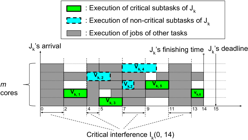
Figure 2. Critical chain and critical interference of $J_{k}$.

Example 4.1.

Figure 2 presents an example of a critical chain of a job $J_{k}$ of task $\tau_{k}$, which has the same DAG as shown in Figure 1. In Figure 2, boxes with bold, solid borders denote the execution of critical subtasks of $J_{k}$; boxes with bold, dashed borders denote the execution of the other subtasks of $J_{k}$. The other boxes are for jobs of other tasks. Subtask $v_{k,6}$ is a last-completing subtask. A last-completing predecessor of $v_{k,6}$ is $v_{k,5}$. Similarly, a last-completing predecessor of $v_{k,5}$ is $v_{k,3}$, and a last-completing predecessor of $v_{k,3}$ is $v_{k,1}$. Hence a critical chain of $J_{k}$ is $(v_{k,1},v_{k,3},v_{k,5},v_{k,6})$.

The critical chain concept has a few properties that make it useful for schedulability analysis of parallel DAG tasks. First, the first subtask of any critical chain of a job is ready to execute as soon as the job is released, since it does not have any predecessor. Second, when the last subtask of a critical chain completes, the corresponding job finishes — this is from the construction of the critical chain. Thus the scheduling window of a critical chain of $J_{k}$ — i.e., from the release time of its first subtask to the completion time of its last subtask — is also the scheduling window of job $J_{k}$ — i.e., from the job’s release time to its completion time. Third, consider a critical chain $\lambda_{k}$ of $J_{k}$: at any instant during the scheduling window of $J_{k}$, either a critical subtask of $\lambda_{k}$ is executed or a critical subtask of $\lambda_{k}$ is ready but not executed because all $m$ processors are busy executing subtasks not belonging to $\lambda_{k}$, including non-critical subtasks of job $J_{k}$ and subtasks from other tasks (see Figure 2). Therefore, the response-time of a critical chain of $J_{k}$ is also the response-time of $J_{k}$. Hence if we can upper-bound the response-time of a critical chain for any job $J_{k}$ of $\tau_{k}$, that bound also serves as an upper-bound for the response-time of $\tau_{k}$.

The third property of the critical chain suggests that we can partition the scheduling window of a job $J_{k}$ into two sets of intervals. One includes all intervals during which critical subtasks of $J_{k}$ are executed and the other includes all intervals during which a critical subtask of $J_{k}$ is ready but not executed. The total length of the intervals in the second set is called the critical interference of $J_{k}$. We include definitions for critical interference and interference caused by an individual task on $\tau_{k}$ as follows.

Definition 4.2.

Critical interference $I_{k}(a,b)$ on a job $J_{k}$ of task $\tau_{k}$ is the aggregated length of all intervals in [a, b) during which a critical subtask of $J_{k}$ is ready but not executed.

Definition 4.3.

Critical interference $I_{i,k}(a,b)$ on a job $J_{k}$ of task $\tau_{k}$ due to task $\tau_{i}$ is the aggregated processor time from all intervals in [a, b) during which one or more subtasks of $\tau_{i}$ are executed and a critical subtask of $J_{k}$ is ready but not executed.

In Figure 2, the critical interference $I_{k}(0,14)$ of $J_{k}$ is the sum of the lengths of intervals $[0,2)$, $[4,5)$, $[7,9)$, and $[11,13)$ which is 7. The critical interference $I_{i,k}(0,14)$ caused by a task $\tau_{i}$ is the total processor time of $\tau_{i}$ in those four intervals. Note that $\tau_{i}$ may execute simultaneously on multiple processors, and we must sum its processor time on all processors. From the definition of critical interference, we have:

(1) $$I_{k}(a,b)=\frac{1}{m}\sum\limits_{\tau_{i}\in\tau}I_{i,k}(a,b).$$

4.2. A General Method for Bounding Response-Time

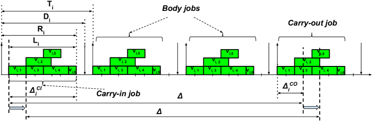
Figure 3. Workload generated by an interfering task $\tau_{i}$ in an interval of length $\Delta$.

We now discuss a general framework for bounding response-time in G-FP that is used in this work and was also employed by the state-of-the-art analyses (Melani et al., 2015; Fonseca et al., 2017). Based on the definitions of critical chain and critical interference, the response-time $R_{k}$ of $J_{k}$ is:

$$R_{k}=len(\lambda_{k})+I_{k}(r_{k},r_{k}+R_{k}),$$

where $\lambda_{k}$ is a critical chain of $J_{k}$ and $len(\lambda_{k})$ is its length (see Figure 2 for example). Applying Equation 1 we have:

(2) $$R_{k}=\Big{(}len(\lambda_{k})+\frac{1}{m}I_{k,k}(r_{k},r_{k}+R_{k})\Big{)}+\frac{1}{m}\sum\limits_{\tau_{i}\in hp(\tau_{k})}I_{i,k}(r_{k},r_{k}+R_{k}),$$

where $hp(\tau_{k})$ is the set of tasks with higher priorities than $\tau_{k}$’s. Thus if we can bound the right-hand side of Equation 2, we can bound the response-time of $\tau_{k}$. To do so, we bound the contributions to $J_{k}$’s response-time caused by subtasks of $J_{k}$ itself and by jobs of higher-priority tasks separately.

4.2.1. Intra-Task Interference

The sum $\Big{(}len(\lambda_{k})+\frac{1}{m}I_{k,k}(r_{k},r_{k}+R_{k})\Big{)}$, which includes the intra-task interference on the critical chain of $J_{k}$ caused by non-critical subtasks of $J_{k}$, is bounded by Lemma V.3 in (Melani et al., 2015). We include the bound below.

Lemma 4.4.

The following inequality holds for any task $\tau_{k}$ scheduled by any work-conserving algorithm:

$$len(\lambda_{k})+\frac{1}{m}I_{k,k}(r_{k},r_{k}+R_{k})\leq L_{k}+\frac{1}{m}(C_{k}-L_{k})$$

4.2.2. Inter-Task Interference

Now we need to bound the inter-task interference on the right-hand side of Equation 2. Since the interference caused by a task in an interval is at most the workload generated by the task during that interval, we can bound $I_{i,k}(a,b),~{}\forall\tau_{i}\in hp(\tau_{k})$ using the bound for the workload generated by $\tau_{i}$ in the interval $[a,b)$. Let $W_{i}(a,b)$ denote the maximum workload generated by $\tau_{i}$ in the interval $[a,b)$. Let $W_{i}(\Delta)$ denote the maximum workload generated by $\tau_{i}$ in any interval of length $\Delta$. The following inequality holds for any $\tau_{i}$:

(3) $$I_{i,k}(r_{k},r_{k}+R_{k})\leq W_{i}(r_{k},r_{k}+R_{k})\leq W_{i}(R_{k}).$$

Let the problem window be the interval of interest with length $\Delta$. The jobs of $\tau_{i}$ that may generate workload within the problem window are classified into three types: (i) A carry-in job is released strictly before the problem window and has a deadline within it, (ii) A carry-out job is released within the problem window and has its deadline strictly after it, and (iii) body jobs have both release time and deadline within the problem window. Similar to analyses for sequential tasks (e.g., Bertogna et al. (Bertogna and Cirinei, 2007)), the maximum workload generated by $\tau_{i}$ in the problem window can be attained with a release pattern in which (i) jobs of $\tau_{i}$ are released as quickly as possible, meaning that the gap between any two consecutive releases is exactly the period $T_{i}$, (ii) the carry-in job finishes as late as its worst-case finishing time, and (iii) the body jobs and the carry-out job start executing as soon as they are released. Figure 3 shows an example of such a job-release pattern of an interfering task $\tau_{i}$ with the DAG structure shown in Figure 1.

However, unlike sequential tasks, analysis for parallel DAG tasks is more challenging in two aspects. First, it is not obvious which schedule for the subtasks of the carry-in (carry-out) job would generate maximum carry-in (carry-out) workload. This is because the parallelism of a DAG task can vary depending on its internal graph structure. Second, for the same reason, aligning the problem window’s start time with the start time of the carry-in job of $\tau_{i}$ may not correspond to the maximum workload generated by $\tau_{i}$. For instance, in Figure 3 if we shift the problem window to the right 2 time units, the carry-in job’s workload loses 2 time units but the carry-out job’s workload gains 5 time units. The total workload thus increases 3 time units. Therefore in order to compute the maximum workload generated by $\tau_{i}$ we must slide the problem window to find a position that corresponds to the maximum sum of the carry-in workload and carry-out workload. We discuss an existing method for computing carry-in workload in Section 5 and our technique for computing carry-out workload in Section 6. In Section 7, we combine those two bounds in a response-time analysis and explain how we slide problem windows to compute maximum workloads.

We note that the maximum workload generated by each body job does not depend on the schedule of its subtasks and is simply its total work. Furthermore, regardless of the position of the problem window, the workload contributed by the body jobs, denoted by $W_{i}^{BO}(\Delta)$, is bounded as follows.

Lemma 4.5.

The workload generated by the body jobs of task $\tau_{i}$ in a problem window with length $\Delta$ is upper-bounded by

$$W_{i}^{BO}(\Delta)=\max\Big{\{}\big{(}\Bigl{\lfloor}\frac{\Delta-L_{i}+R_{i}}{T_{i}}\Bigr{\rfloor}-1\big{)}C_{i},0\Big{\}}.$$

Proof.

Consider the case where the start of the problem window is aligned with the starting time of the carry-in job, as shown in Figure 3. The number of body jobs is at most $\max\big{\{}\Bigl{\lfloor}\frac{\Delta-L_{i}+R_{i}}{T_{i}}\Bigr{\rfloor}-1,0\big{\}}$. Thus for this case the workload of the body jobs is at most $\max\big{\{}\big{(}\Bigl{\lfloor}\frac{\Delta-L_{i}+R_{i}}{T_{i}}\Bigr{\rfloor}-1\big{)}C_{i},0\big{\}}$.

Shifting the problem window to the left or right can change the workload contributed by the carry-in and carry-out jobs but does not increase the maximum number of body jobs or their workload. The bound thus follows. ∎

Let the carry-in window and carry-out window be the intervals within the problem window during which the carry-in job and the carry-out job are executed, respectively. Intuitively, the carry-in window spans from the start of the problem window to the completion time of the carry-in job; the carry-out window spans from the starting time of the carry-out job to the end of the problem window. We denote the lengths of the carry-in window and carry-out window for task $\tau_{i}$ by $\Delta_{i}^{CI}$ and $\Delta_{i}^{CO}$ respectively. The sum of $\Delta_{i}^{CI}$ and $\Delta_{i}^{CO}$ is:

(4) $$\Delta_{i}^{CI}+\Delta_{i}^{CO}=L_{i}+(\Delta-L_{i}+R_{i})\mod T_{i}$$

Let $W_{i}^{CI}(\Delta_{i}^{CI})$ be the maximum carry-in workload of $\tau_{i}$ for a carry-in window of length $\Delta_{i}^{CI}$. Similarly, let $W_{i}^{CO}(\Delta_{i}^{CO})$ be the maximum carry-out workload of $\tau_{i}$ for a carry-out window of length $\Delta_{i}^{CO}$. The maximum workload generated by $\tau_{i}$ in any problem window of length $\Delta$ can be computed by taking the maximum over all $\Delta_{i}^{CI}$ and $\Delta_{i}^{CO}$ that satisfy Equation 4:

(5) $$W_{i}(\Delta)=W_{i}^{BO}(\Delta)+\max\limits_{\Delta_{i}^{CI},\Delta_{i}^{CO}\text{satisfy Eq.~{}\ref{eqn:ci_co_length}}}\Big{\{}W_{i}^{CI}(\Delta_{i}^{CI})+W_{i}^{CO}(\Delta_{i}^{CO})\Big{\}}.$$

Therefore if we can bound $W_{i}^{CI}(\Delta_{i}^{CI})$ and $W_{i}^{CO}(\Delta_{i}^{CO})$, we can bound the inter-task interference of $\tau_{i}$ on $\tau_{k}$ and thus the response-time of $\tau_{k}$.

5. The State-of-the-Art Analysis for G-FP

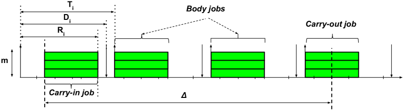
Figure 4. Workload generated by an interfering task $\tau_{i}$ in Melani et al. (Melani et al., 2015).

Melani et al. (Melani et al., 2015) proposed a response-time analysis for G-FP scheduling of conditional DAG tasks that may contain conditional vertices, for modeling conditional constructs such as if-then-else statements. They bounded the interfering workload by assuming that jobs of the interfering task execute perfectly in parallel on all $m$ processors. Their bound for the interfering workload is computed as follows.

$$W_{i}(\Delta)=\Big{\lfloor}\frac{\Delta+R_{i}-C_{i}/m}{T_{i}}\Big{\rfloor}C_{i}+\min\big{\{}C_{i},m((\Delta+R_{i}-C_{i}/m)\mod T_{i})\big{\}}.$$

Figure 4 illustrates the workload computation for an interfering task $\tau_{i}$ given in (Melani et al., 2015). As shown in this figure, both carry-in and carry-out jobs are assumed to execute with perfect parallelism upon $m$ processors. Thus their workload contributions in the considered window are maximized. This assumption simplifies the workload computation as it ignores the internal DAG structures of the interfering tasks. However, assuming that DAG tasks have such abundant parallelism is likely unrealistic and thus makes the analysis pessimistic.

Fonseca et al. (Fonseca et al., 2017) later considered a task model similar to the one in this paper and proposed a method to improve the bounds for carry-in and carry-out workloads by explicitly considering the DAGs. The carry-in workload was bounded using a hypothetical schedule for the carry-in job, in which the carry-in job can use as many processors as it needs to fully exploit its parallelism. They proved that the carry-in workload of the hypothetical schedule is maximized when: (i) the hypothetical schedule’s completion time is aligned with the worst-case completion time of the interfering task, (ii) every subtask in the hypothetical schedule starts executing as soon as all of its predecessors finish, and (iii) every subtask in the hypothetical schedule executes for its full WCET. Figure 3 shows the hypothetical schedule of the carry-in job for the task in Figure 1. In this paper, we adopt their method for computing carry-in workload. In particular, the carry-in workload of task $\tau_{i}$ with a carry-in window of length $\Delta_{i}^{CI}$, i.e., from the start of the problem window to the completion time of the carry-in job (see Figure 3), is computed as follows.

(6) $$W_{i}^{CI}(\Delta_{i}^{CI})=\sum_{v_{i,k}\in V_{i}}\max\big{\{}C_{i,k}-\max(L_{i}-S_{i,k}-\Delta_{i}^{CI},0),0\big{\}}.$$

In Equation 6, $S_{i,k}$ is the start time of subtask $v_{i,k}$ in the hypothetical schedule for the carry-in job described above. It can be computed by taking a longest path among all paths from source subtasks to $v_{i,k}$ and adding up the WCETs of the subtasks along that path excluding $v_{i,k}$ itself.

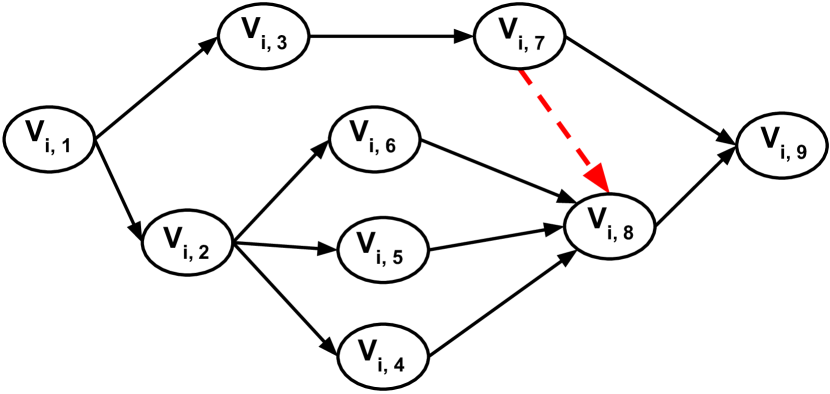
(a) A non-nested-fork-join DAG task.

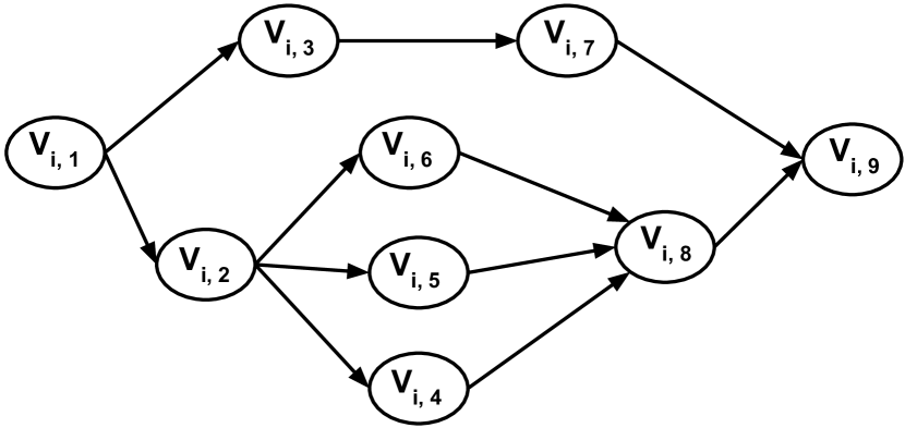
(b) A nested fork-join DAG task.

Figure 5. Example for a general DAG task and a nested fork-join DAG task.

For the carry-out workload, (Fonseca et al., 2017) considered a subset of generalized DAG tasks, namely nested fork-join DAG (NFJ-DAG) tasks. A NFJ-DAG is constructed recursively from smaller NFJ-DAGs using two operations: series composition and parallel composition. Figure 5(b) shows an example NFJ-DAG task. Figure 5(a) shows a similar DAG with one more edge $(v_{i,7},v_{i,8})$. The DAG in Figure 5(a) is not a NFJ-DAG due to a single cross edge $(v_{i,7},v_{i,8})$. To deal with a non NFJ-DAG, (Fonseca et al., 2017) first transforms the original DAG to a NFJ-DAG by removing the conflicting edges, such as $(v_{i,7},v_{i,8})$ in Figure 5. Then they compute the upper-bound for the carry-out workload using the obtained NFJ-DAG. The computed bound is proved to be an upper-bound for the carry-out workload. We note that the transformation removes some precedence constraints from the original DAG, and thus the resulting NFJ-DAG may have higher parallelism than the original DAG. Hence, computing the carry-out workload of a generalized DAG task via its transformed NFG-DAG may be pessimistic, especially for a complex DAG, as the transformation may remove many edges from the original DAG.

In this paper, we propose a new technique to directly compute an upper-bound for the carry-out workload of generalized DAG task. The high level idea is to frame the problem of finding the bound as an optimization problem, which can be solved effectively by solvers such as the CPLEX (IBM ILOG CPLEX Optimizer, 2019), Gurobi (Gurobi Solver, 2019), or SCIP (SCIP Solver, 2019). The solution of the optimization problem then serves as a safe and tight upper-bound for the carry-out workload. In the next section we present our method in detail.

6. Bound for Carry-Out Workload

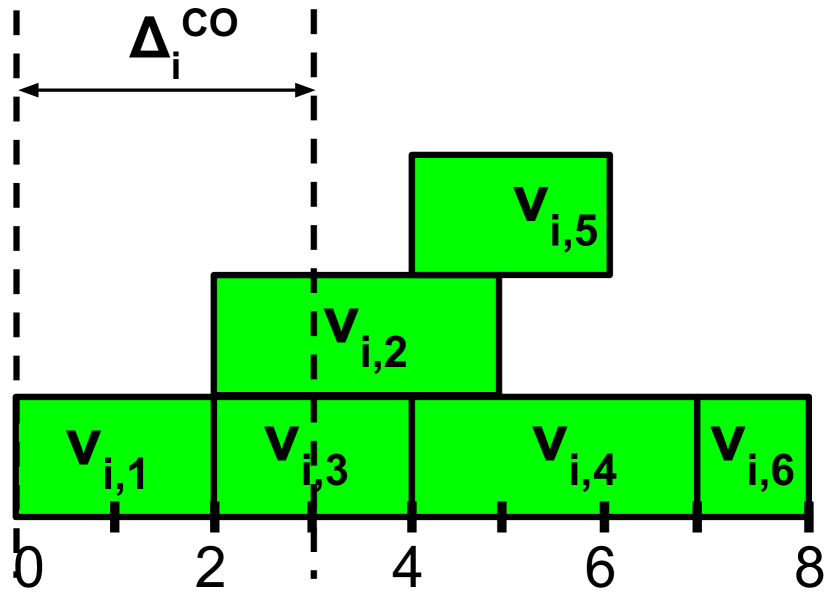
(a) Carry-out workload when all subtasks execute for WCETs.

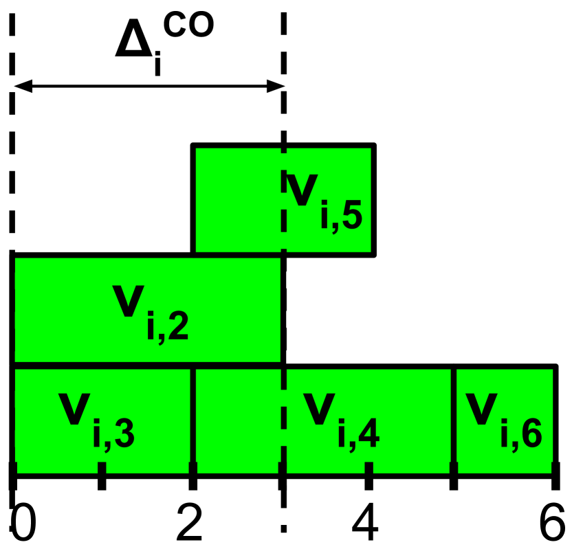
(b) Carry-out workload when subtasks may execute less than WCETs.

Figure 6. An illustration of generating the maximum carry-out workload.

In this section we propose a method to bound the carry-out workload that can be generated by a job of task $\tau_{i}$ by constructing an integer linear program (ILP) for which the optimal solution value is an upper-bound of the carry-out workload.

Consider a carry-out job of task $\tau_{i}$, which is scheduled with an unrestricted number of processors, meaning that it can use as many processors as it requires to fully exploit its parallelism. Each subtask of the carry-out job executes as soon as it is ready, i.e., immediately after all of its predecessors have finished. We label such a schedule for the carry-out job $\mathcal{SCHE}^{CO}(\tau_{i})$. We prove in the following lemma that the workload generated by $\mathcal{SCHE}^{CO}(\tau_{i})$ is an upper-bound for the carry-out workload.

Lemma 6.1.

For specific values of the execution times for the subtasks of $\tau_{i}$, workload generated by $\mathcal{SCHE}^{CO}(\tau_{i})$ in a carry-out window of length $\Delta_{i}^{CO}$ is an upper-bound for the carry-out workload generated by $\tau_{i}$ with the given subtasks’s execution times.

Proof.

We prove by contradiction. Consider a schedule $\mathcal{SCHE}^{*}$ for the carry-out job in which subtasks execute for the same lengths as in $\mathcal{SCHE}^{CO}(\tau_{i})$. Suppose subtask $v_{i,k}$ is the first subtask in time order that produces more workload in $\mathcal{SCHE}^{*}$ than it does in $\mathcal{SCHE}^{CO}(\tau_{i})$. This means $v_{i,k}$ must have started executing earlier in $\mathcal{SCHE}^{*}$ than it have in $\mathcal{SCHE}^{CO}(\tau_{i})$. Hence, $v_{i,k}$ must have started its execution before all of its predecessors have finished in $\mathcal{SCHE}^{*}$. This is impossible and the lemma follows. ∎

Unlike the carry-in workload, the carry-out workload generated when all subtasks execute for their full WCETs is not guaranteed to be the maximum. Consider an interfering task $\tau_{i}$ shown in Figure 1 and a carry-out window of length 3 time units. If all subtasks of the carry-out job of $\tau_{i}$ execute for their WCETs, the carry-out workload would be 4 time units, as shown in Figure 6(a). However, if subtask $v_{i,1}$ finishes immediately, i.e., executes for 0 time units, the carry-out workload would be 7 time units, as shown in Figure 6(b). From Lemma 6.1 and the discussion above, to compute an upper-bound for carry-out workload we must consider all possible execution times of the subtasks and subtasks must execute as soon as they are ready.

For each subtask $v_{i,a}$ of the carry-out job of an interfering task $\tau_{i}$, we define two non-negative integer variables $X_{i,a}\geq 0$ and $W_{i,a}\geq 0$. $X_{i,a}$ represents the actual execution time of subtask $v_{i,a}$ in the carry-out job and $W_{i,a}$ denotes the contribution of subtask $v_{i,a}$ to the carry-out workload. Let $\Delta^{CO}$ be an integer constant denoting the length of the carry-out window. Then the carry-out workload is the sum of the contributions of all subtasks in $\mathcal{SCHE}^{CO}(\tau_{i})$, which is upper-bounded by the maximum of the following optimization objective function:

(7) $$obj(\tau_{i},\Delta^{CO})\triangleq\sum\limits_{v_{i,a}\in V_{i}}W_{i,a}.$$

The optimal value for the above objective function gives the actual maximum workload generated by the carry-out job with unrestricted number of processors. We now construct a set of constraints on the contribution of each subtask in $\mathcal{SCHE}^{CO}(\tau_{i})$ to the carry-out workload. From the definitions of $X_{i,a}$ and $W_{i,a}$, we have the following bounds for them.

Constraint 1.

For any interfering task $\tau_{i}$:

$$\forall v_{i,a}\in V_{i}:0\leq X_{i,a}\leq C_{i,a}.$$

Constraint 2.

For any interfering task $\tau_{i}$:

$$\forall v_{i,a}\in V_{i}:0\leq W_{i,a}\leq X_{i,a}.$$

These two constraints come from the fact that the actual execution time of subtask $v_{i,a}$ cannot exceed its WCET, and each subtask can contribute at most its whole execution time to the carry-out workload. Let $S_{i,a}$ be the starting time of $v_{i,a}$ in $\mathcal{SCHE}^{CO}(\tau_{i})$ assuming that the carry-out job starts at time instant 0. For simplicity of exposition, we assume that the DAG $G_{i}$ has exactly one source vertex and one sink vertex. If this is not the case, we can always add a couple of dummy vertices, $v_{i,source}$ and $v_{i,sink}$, with zero WCETs for source and sink vertices, respectively. Then we add edges from $v_{i,source}$ to all vertices with no predecessors in the original DAG $G_{i}$, and edges from all vertices with no successors in $G_{i}$ to $v_{i,sink}$. Without loss of generality, we assume that $v_{i,1}$ and $v_{i,n_{i}}$ are the source vertex and sink vertex of $G_{i}$, respectively. Let $\sigma^{p}_{i,a}$ denote a path from the source $v_{i,1}$ to $v_{i,a}$: $\sigma^{p}_{i,a}\triangleq(v_{i,j_{1}},...,v_{i,j_{p}})$, where $j_{1}=1$, $j_{p}=a$, and $(v_{i,j_{x}},v_{i,j_{x+1}})$ is an edge in $G_{i}$ $\forall 1\leq x<p$. Let $\mathcal{P}(v_{i,a})$ denote the set of all paths from $v_{i,1}$ to $v_{i,a}$ in $G_{i}$: $\mathcal{P}(v_{i,a})\triangleq\{\sigma^{p}_{i,a}\}$. $\mathcal{P}(v_{i,a})$ for all subtasks can be constructed by a graph traversal algorithm. For instance, a simple modification of depth-first search would accomplish this.

For a particular path $\sigma^{p}_{i,a}$, the sum of execution times of all subtasks in this path, excluding $v_{i,a}$ is called the distance to $v_{i,a}$ with respect to this path. We let $D^{p}_{i,a}$ be a variable denoting the distance to $v_{i,a}$ in path $\sigma^{p}_{i,a}$. We impose the following two straightforward constraints on $D^{p}_{i,a}$ based on its definition.

Constraint 3.

For any interfering task $\tau_{i}$:

$$\forall v_{i,a}\in V_{i},\forall\sigma^{p}_{i,a}\in\mathcal{P}(v_{i,a}):D^{p}_{i,a}\leq\sum\limits_{v_{i,j_{x}}\in\{\sigma^{p}_{i,a}\setminus v_{i,a}\}}X_{i,j_{x}}.$$

Constraint 4.

For any interfering task $\tau_{i}$:

$$\forall v_{i,a}\in V_{i},\forall\sigma^{p}_{i,a}\in\mathcal{P}(v_{i,a}):D^{p}_{i,a}\geq\sum\limits_{v_{i,j_{x}}\in\{\sigma^{p}_{i,a}\setminus v_{i,a}\}}X_{i,j_{x}}.$$

In the schedule $\mathcal{SCHE}^{CO}(\tau_{i})$, the starting time $S_{i,a}$ of a subtask $v_{i,a}$ cannot be smaller than the distance to $v_{i,a}$ in any path $\sigma^{p}_{i,a}$. We prove this as follows.

Lemma 6.2.

In the schedule $\mathcal{SCHE}^{CO}(\tau_{i})$ of any interfering task $\tau_{i}$:

$$\forall v_{i,a}\in V_{i},\forall\sigma^{p}_{i,a}\in\mathcal{P}(v_{i,a}):S_{i,a}\geq D^{p}_{i,a}.$$

Proof.

We prove by contradiction. Let $\sigma^{p*}_{i,a}$ be a path so that the starting time $S_{i,a}$ is smaller than $D^{p*}_{i,a}$. Subtask $v_{i,a}$ must be ready to start execution, meaning all of its predecessors must finish, at time $S_{i,a}$. Since $S_{i,a}<D^{p*}_{i,a}$, there must be a subtask $v_{i,j_{x}}\in\{\sigma^{p*}_{i,a}\setminus v_{i,a}\}$ executing (and thus not finished) at time $S_{i,a}$. Then $v_{i,a}$ cannot be ready at time $S_{i,a}$ since it depends on $v_{i,j_{x}}$. This contradicts the assumption that $v_{i,a}$ is ready at $S_{i,a}$ and the lemma follows. ∎

In fact, in the schedule $\mathcal{SCHE}^{CO}(\tau_{i})$ the starting time $S_{i,a}$ of $v_{i,a}$ is equal to the longest distance among all paths to it.

Lemma 6.3.

In the schedule $\mathcal{SCHE}^{CO}(\tau_{i})$ of any interfering task $\tau_{i}$:

$$\forall v_{i,a}\in V_{i}:S_{i,a}=\max\limits_{\sigma^{p}_{i,a}\in\mathcal{P}(v_{i,a})}D^{p}_{i,a}.$$

Proof.

Consider a path $\sigma^{p*}_{i,a}$ constructed as follows. First we take a last-completing predecessor of $v_{i,a}$, say $v_{i,j_{x}}$. Since $v_{i,a}$ executes as soon as it is ready, it executes immediately after $v_{i,j_{x}}$ finishes. We recursively trace back through the last-completing predecessors in that way until we reach the source vertex $v_{i,1}$. Path $\sigma^{p*}_{i,a}$ is then constructed by chaining the last-completing predecessors together with $v_{i,a}$. We note that any subtask $v_{i,j_{x}}$ in $\sigma^{p*}_{i,a}$ executes as soon as its immediately preceding subtask finishes, since no other predecessors of $v_{i,j_{x}}$ finish later than it does. Therefore, $S_{i,a}=D^{p*}_{i,a}$. From Lemma 6.2, $\sigma^{p*}_{i,a}$ must have the longest distance to $v_{i,a}$ among all paths in $\mathcal{P}(v_{i,a})$. Thus the lemma follows. ∎

Based on Lemmas 6.2 and 6.3, we have the following constraint for the starting time of $v_{i,a}$.

Constraint 5.

For any interfering task $\tau_{i}$:

$$\forall v_{i,a}\in V_{i},\forall\sigma^{p}_{i,a}\in\mathcal{P}(v_{i,a}):S_{i,a}\geq D^{p}_{i,a}.$$

Proof.

We prove that this constraint requires that $S_{i,a}$ of every subtask $v_{i,a}$ for which $\max_{\sigma^{p}_{i,a}\in\mathcal{P}(v_{i,a})}D^{p}_{i,a}<\Delta^{CO}$ satisfies Lemma 6.3, that is $S_{i,a}=\max_{\sigma^{p}_{i,a}\in\mathcal{P}(v_{i,a})}D^{p}_{i,a}$. (Recall that $\Delta^{CO}$ is a constant denoting the carry-out window’s length.) In other words, we prove that it requires that every subtask $v_{i,a}$, which would start executing within the carry-out window in an unrestricted-processor schedule $\mathcal{SCHE}^{CO}(\tau_{i})$, gets exactly the same starting time from the solution to the optimization problem. Let $\mathcal{Q}_{i}$ denote the collection of such subtasks — the ones that would start executing within the carry-out window in $\mathcal{SCHE}^{CO}(\tau_{i})$.

Let $\pi^{*}$ be the solution to the optimization problem and $S^{*}_{i,a}$ be the corresponding value for the starting time of any subtask $v_{i,a}\in\mathcal{Q}_{i}$ in the solution $\pi^{*}$. Obviously $S^{*}_{i,a}\geq\max_{\sigma^{p}_{i,a}\in\mathcal{P}(v_{i,a})}D^{p}_{i,a}$ for any $v_{i,a}$ since any solution to the optimization problem satisfies this constraint. If $S^{*}_{i,a}=\max_{\sigma^{p}_{i,a}\in\mathcal{P}(v_{i,a})}D^{p}_{i,a}$ for any $v_{i,a}\in\mathcal{Q}_{i}$, then we are done. Suppose instead that $S^{*}_{i,a}=\max_{\sigma^{p}_{i,a}\in\mathcal{P}(v_{i,a})}D^{p}_{i,a}+\epsilon_{i,a}$, $\epsilon_{i,a}>0$ for some $v_{i,a}\in\mathcal{Q}_{i}$. Let $\mathcal{Q^{\prime}}_{i}$ denote the set of such subtasks. We construct a solution $\pi^{\prime}$ to the optimization problem from $\pi^{*}$ as follows. Consider a first subtask $v_{i,a}\in\mathcal{Q^{\prime}}_{i}$ in time. We reduce its starting time by $\epsilon_{i,a}$: $S^{\prime}_{i,a}=S^{*}_{i,a}-\epsilon_{i,a}$. Since $v_{i,a}$ is the first delayed subtask, doing this does not violate the precedence constraints for other subtasks. We iteratively perform that operation for other subtasks in $\mathcal{Q^{\prime}}_{i}$ in increasing time order. The solution $\pi^{\prime}$ constructed in this way yields a larger carry-out workload since more workload from individual subtasks can fit in the carry-out window. Therefore $\pi^{\prime}$ is a better solution, which contradicts the assumption that $\pi^{*}$ is an optimal solution. ∎

The workload contributed by a subtask $v_{i,a}$ is:
$W_{i,a}=\min\big{\{}\max\{\Delta^{CO}-S_{i,a},0\},X_{i,a}\big{\}}$. The second part of the outer minimization has been taken care of by Constraint 2. We now construct constraints to impose the first part of the minimization. Let $M_{i,a}$ be an integer variable representing the expression $\max\{\Delta^{CO}-S_{i,a},0\}$. Let $A_{i,a}$ be a binary variable which takes value either 0 or 1. We have the following constraints.

Constraint 6.

For any interfering task $\tau_{i}$:

$$\forall v_{i,a}\in V_{i}:W_{i,a}\leq M_{i,a}.$$

Constraint 7.

For any interfering task $\tau_{i}$:

$$\forall v_{i,a}\in V_{i}:M_{i,a}\geq 0.$$

Constraint 8.

For any interfering task $\tau_{i}$:

$$\forall v_{i,a}\in V_{i}:M_{i,a}\leq(\Delta^{CO}-S_{i,a})A_{i,a}.$$

Constraints 7 and 8 bound the value for $M_{i,a}$ and Constraint 6 enforces another upper bound for the workload $W_{i,a}$. If $\Delta^{CO}<S_{i,a}$, $A_{i,a}$ can only be 0 in order to satisfy both Contraints 7 and 8. If $\Delta^{CO}=S_{i,a}$, the value of $A_{i,a}$ does not matter. In both cases, these three constraints together with Constraint 2 bound $W_{i,a}$ to zero contribution of $v_{i,a}$ to the carry-out workload. If $\Delta^{CO}>S_{i,a}$, the maximizing process enforces that $A_{i,a}$ takes value 1. Therefore in any case Constraints 2, 6, 7, and 8 enforce a correct value for the workload contribution $W_{i,a}$ of $v_{i,a}$.

We have constructed an ILP with a quadratic constraint (Constraint 8) for each $v_{i,a}$, for which the optimal solution value is an upper bound for the carry-out workload. The carry-out workload of $\tau_{i}$ in a carry-out window of length $\Delta^{CO}$ can also be upper-bounded by the following straightforward lemma.

Lemma 6.4.

The carry-out workload of an interfering task $\tau_{i}$ scheduled by G-FP in a carry-out window of length $\Delta^{CO}$ is upper-bounded by $m\Delta^{CO}$.

Lemma 6.4 follows directly from the fact that the carry-out job can execute at most on all $m$ processors of the system during the carry-out window. Since the carry-out workload of $\tau_{i}$ is upper-bounded by both the maximum value returned for the optimization problem and Lemma 6.4, it is upper-bounded by the minimum of the two quantities.

Theorem 6.5.

The carry-out workload of an interfering task $\tau_{i}$ scheduled by G-FP in a carry-out window of length $\Delta^{CO}$ is upper-bounded by: $\min\Big{\{}\mathcal{OBJ},m\Delta^{CO}\Big{\}}$, where $\mathcal{OBJ}$ is the maximum value returned for the maximization problem (Equation 7).

As discussed in Section 5, the technique proposed by Fonseca et al. (Fonseca et al., 2017) can be applied directly for NFJ-DAGs but not for general DAGs. For a general DAG, the procedure to transform the general DAG to an NFJ-DAG will likely inflate the carry-out workload bound as it removes some precedence constraints between subtasks and enables a higher parallelism (and thus a greater interfering workload) for the carry-out job. In contrast, our method directly bounds the carry-out workload for any DAG and the optimal value obtained is the actual maximum carry-out workload. Hence, our method theoretically yields better schedulability than (Fonseca et al., 2017)’s for general DAGs. The cost of our method is higher time complexity for computing carry-out workload due to the hardness of the ILP problem. However, it can be implemented and works effectively with modern optimization solvers, as we show in our experiments (Section 8).

7. Response-Time Analysis

Algorithm 1 Response-Time Analysis

1:procedure SchedulabilityTest($\tau$) $\triangleright$ Without loss of generality, assuming tasks are sorted in decreasing order of priority

2:     for Each $\tau_{k}\in\tau$ do $\triangleright$ Initialize the values for response-time bounds

3:         $R_{k}^{ub}\leftarrow L_{k}+\frac{1}{m}(C_{k}-L_{k})$

4:         if Any $R_{k}^{ub}>D_{k}$ then

5:              Return Unschedulable

6:         end if

7:     end for

8:

9:     for $\tau_{k}$ from $\tau_{2}$ to $\tau_{n}$ do

10:         Calculate $R_{k}^{ub}$ in Theorem 7.1

11:         if $R_{k}^{ub}>D_{k}$ then

12:              Return Unschedulable

13:         end if

14:     end for

15:     Return Schedulable

16:end procedure

From the above calculations for the bounds of intra-task interference and inter-task interference on $\tau_{k}$, we have the following theorem for the response-time bound of $\tau_{k}$.

Theorem 7.1.

A constrained-deadline task $\tau_{k}$ scheduled by a global fixed-priority algorithm has response-time upper-bounded by the smallest integer $R_{k}^{ub}$ that satisfies the following fixed-point iteration:

$$R_{k}^{ub}\leftarrow L_{k}+\frac{1}{m}(C_{k}-L_{k})+\frac{1}{m}\sum\limits_{\tau_{i}\in hp(\tau_{k})}W_{i}(R_{k}^{ub}).$$

Proof.

This follows from Equation 2, Lemma 4.4 and the fact that the inter-task interference of $\tau_{i}$ on $\tau_{k}$ is bounded by the workload generated by $\tau_{i}$ (Equation 3). ∎

In Theorem 7.1, $W_{i}(R_{k}^{ub})$ is computed using Equation 5 for all carry-in and carry-out windows that satisfy Equation 4. For specific carry-in and carry-out window lengths, the carry-in workload is bounded using Equation 6 and the carry-out workload is bounded as discussed in Section 6. The lengths for carry-in window $\Delta_{i}^{CI}$ and carry-out window $\Delta_{i}^{CO}$ are varied as follows. Let $\Gamma$ denote the right-hand side of Equation 4. First $\Delta_{i}^{CI}$ takes its largest value: $\Delta_{i}^{CI}\leftarrow\min\{\Gamma,L_{i}\}$, and $\Delta_{i}^{CO}$ takes the remaining sum: $\Delta_{i}^{CO}\leftarrow\min\{\Gamma-\Delta_{i}^{CI},L_{i}\}$. Then in each subsequent step, $\Delta_{i}^{CI}$ is decreased and $\Delta_{i}^{CO}$ is increased until $\Delta_{i}^{CO}$ takes its largest value and $\Delta_{i}^{CI}$ takes the remaining value. We note that if at the first step both $\Delta_{i}^{CI}$ and $\Delta_{i}^{CO}$ are greater than or equal to $L_{i}$, the carry-in workload and carry-out workload are bounded by $\min(C_{i},m\Delta_{i}^{CI})$ and $\min(C_{i},m\Delta_{i}^{CO})$, respectively. Similarly, if the sum of $\Delta_{i}^{CI}$ and $\Delta_{i}^{CO}$ is 0 in Equation 4, both the carry-in workload and the carry-out workload are 0. We also note that for the highest priority task, there is no interference from any other task, and thus its response-time bound can be computed simply by: $R_{k}^{ub}\leftarrow\big{(}L_{k}+\frac{1}{m}(C_{k}-L_{k})\big{)}$.

Using the above response-time bound, we derive a schedulability test, shown in Algorithm 1. First we initialize the response-times for the tasks to be $\big{(}L_{k}+\frac{C_{k}-L_{k}}{m}\big{)}$ for all tasks $\tau_{k}$. If for any task, the initial response-time is larger than its relative deadline, then the task set is deemed unschedulable (lines 2-7). Otherwise, we repeatedly compute the response-time bound for each task in descending order of priority using the fixed-point iteration in Theorem 7.1 (line 10). After the computation for each task finishes, we check whether the response-time bound is larger than its deadline. If it is, then the task set is deemed unschedulable (lines 11-13). Otherwise, the task set is deemed schedulable after all tasks have been checked (line 15).

As expected for response-time analysis, for each task $\tau_{i}$ the number of iterations in the fixed-point equation (Theorem 7.1) is pseudo-polynomial in the task’s deadline $D_{i}$ (line 10). In each iteration of the fixed-point equation and for each interfering task, we consider all combinations of carry-in and carry-out window lengths that satisfy Equation 4 to compute the maximum interfering workload. There are $\mathcal{O}(L_{i})$ such combinations, and thus the ILP for the carry-out workload is solved $\mathcal{O}(L_{i})$ times. The maximum workload over all combinations of carry-in and carry-out window lengths gives an upper-bound for the interfering workload generated by the given interfering task.

8. Evaluation

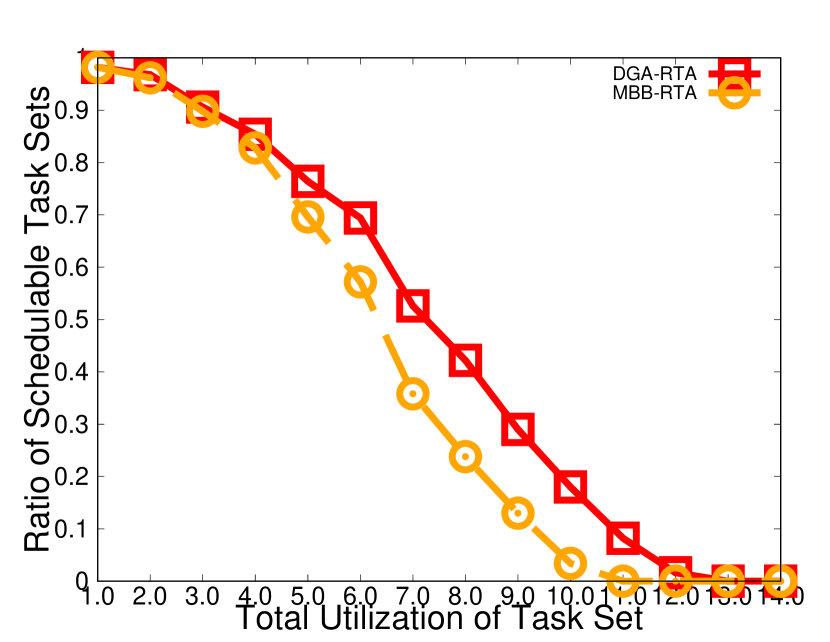
(a) Result for $m=16$, minimum task utilization $\beta=0.2$, and varying total utilization.

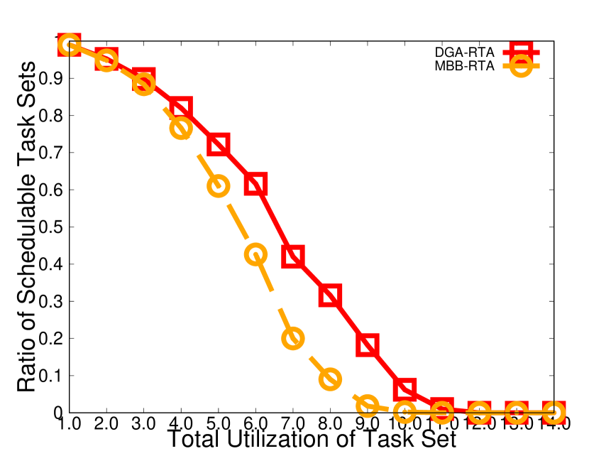
(b) Result for $m=16$, minimum task utilization $\beta=0.4$, and varying total utilization.

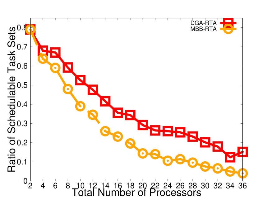
(c) Result for total utilization $U=0.5m$, minimum utilization $\beta=0.1$, and varying $m$.

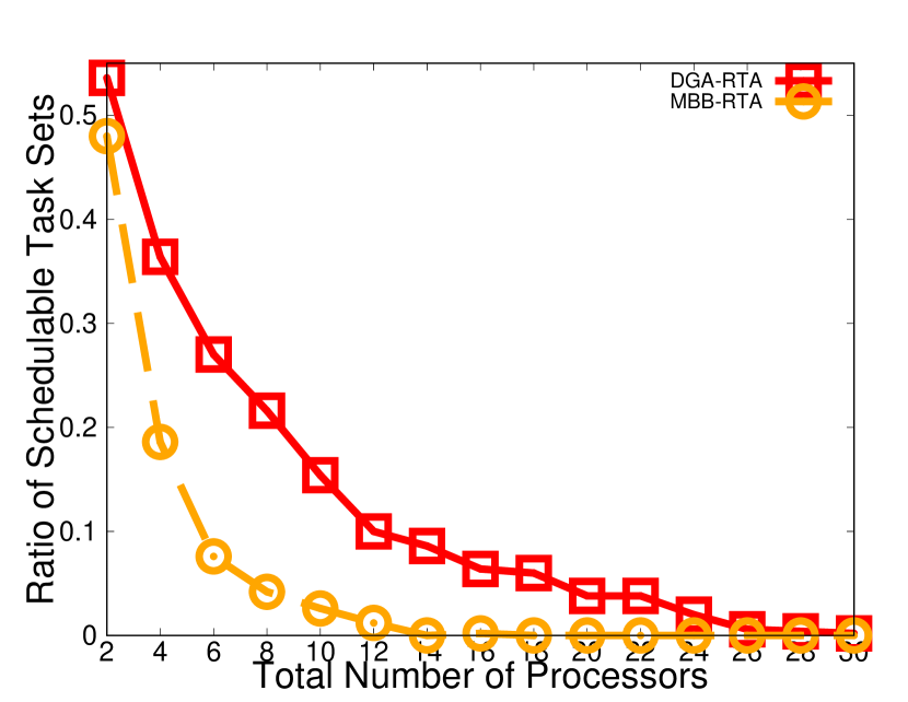
(d) Result for total utilization $U=0.7m$, minimum utilization $\beta=0.1$, and varying $m$.

Figure 7. Ratio of schedulable task sets for varying total utilization and varying number of processors.

As we discussed in Sections 5 and 6, we apply a similar, high-level framework for analyzing schedulability of G-FP scheduling to the one used by Fonseca et al. (Fonseca et al., 2017) — i.e., accounting for the interfering workloads caused by the body jobs, the carry-in and carry-out jobs separately, and maximizing the interference by sliding the problem window. However, unlike (Fonseca et al., 2017) our technique for bounding carry-out workload works directly for general DAGs and does not introduce pessimism due to the removal of precedence constraints between subtasks, as presented in (Fonseca et al., 2017). Though for carry-in workload, we reuse the result from (Fonseca et al., 2017). Hence, we consider our work as a generalization/extension of (Fonseca et al., 2017) that can be applied for general sporadic DAG tasks. The performance of our method in term of schedulability ratio is compatible with (Fonseca et al., 2017)’s — it theoretically is at least as good as (Fonseca et al., 2017) for NFJ-DAGs and is better than (Fonseca et al., 2017) for non NFJ-DAGs. We thus focus on measuring the performance of our method and use the work by Melani et al. (Melani et al., 2015) as a reference for evaluating the improvement of our method upon their simple one.

We applied the Erdős-Rényi $G(n,p)$ method, described in (Cordeiro et al., 2010), to generate DAG tasks. In this method the number of subtasks, given by parameter $n$ in $G(n,p)$, is first fixed. Then, directed edges between pairs of vertices are added with probability $p$. Since the obtained DAG may not necessarily be connected, we added a minimum number of edges to make it weakly connected. In our experiments, the probability for a directed edge to be added is $p=0.2$. We chose the number of subtasks uniformly in the range $[10,20]$. Other parameters for each DAG task $\tau_{i}$ were generated similarly to (Melani et al., 2015). In particular, the WCETs of subtasks of $\tau_{i}$ were generated uniformly in the range $[1,100]$. After that, the work $C_{i}$ and span $L_{i}$ were calculated. $\tau_{i}$’s utilization was generated uniformly in the range $[\beta,C_{i}/L_{i}]$, where $\beta\leq 1$ is a parameter to control the minimum task’s utilization and $C_{i}/L_{i}$ represents the degree of parallelism of task $\tau_{i}$. $\tau_{i}$’s deadline $D_{i}$ was generated using a normal distribution with mean equal to $(\frac{T_{i}+L_{i}}{2})$ and standard deviation equal to $(\frac{T_{i}-L_{i}}{4})$. We kept generating the relative deadline until a value in the range $[L_{i},T_{i}]$ was obtained.

To generate a task set for a given total utilization, we repeatedly add DAG tasks to the task set until the desired utilization is reached. The utilization (and period) of the last task may need to be adjusted to match the total utilization. We used the SCIP solver (SCIP Solver, 2019) with CPLEX (IBM ILOG CPLEX Optimizer, 2019) as its underlying LP-solver to compute the bound for carry-out workload. For our experiments, we set the default minimum utilization of individual tasks $\beta$ to $0.1$. For each configuration we generated 500 task sets and recorded the ratios of task sets that were deemed schedulable. We compare our response-time analysis, denoted by DGA-RTA, with the response-time analysis introduced in (Melani et al., 2015), denoted by MBB-RTA. For all generated task sets, priorities were assigned in Deadline Monotonic order — studying an efficient priority assignment scheme for G-FP is beyond the scope of this paper.

Figures 7(a), 7(b), 7(c), and 7(d) show representative results for our experiments. In Figure 7(a) and 7(b), we fixed the total number of processors $m=16$ and varied the total utilization from 1.0 to 14.0. The minimum task utilization $\beta$ was set to $0.2$ and $0.4$ in these two experiments, respectively. Unsurprisingly, DGA-RTA dominates MBB-RTA, as also observed in (Fonseca et al., 2017). Notably, its schedulability ratios for some configurations are two times or more greater than MBB-RTA, e.g., for total utilizations of 8.0, 9.0 in Figure 7(a), and 7.0, 8.0 in Figure 7(b). In Figures 7(c) and 7(d), we fixed the normalized total utilization and varied the number of processors $m$ from 2 to 36. For each value of $m$, we generated task sets with total utilization $U=0.5m$ or $U=0.7m$ for these two experiments, respectively. Similar to the previous experiments, the schedulability ratios of the generated task sets were improved significantly using DGA-RTA compared to MBB-RTA.

To provide a trade-off between computational complexity and accuracy of schedulability test, one can employ our analysis in combination with the analysis presented in (Fonseca et al., 2017) by first applying their response-time analysis and then using our analysis if the task set is deemed unschedulable by (Fonseca et al., 2017). In this way, one can get the best result from both analyses.

9. Conclusion

In this paper we consider constrained-deadline, parallel DAG tasks scheduled under a preemptive, G-FP scheduling algorithm on multiprocessor platforms. We propose a new technique for bounding carry-out workload of interfering task by converting the calculation of the bound to an optimization problem, for which efficient solvers exist. The proposed technique applies directly to general DAG tasks. The optimal solution value for the optimization problem serves as a safe and tight upper bound for carry-out workload. We present a response-time analysis for G-FP based on the proposed workload bounding technique. Experimental results affirm the dominance of the proposed approach over existing techniques. There are a couple of open questions that we would like to address in future. They include bounding carry-in and carry-out workloads for the actual number of processors $m$ of the system and designing an efficient priority assignment scheme for parallel DAG tasks scheduled under G-FP algorithm.

References

- (1)
- Axer et al. (2013) Philip Axer, Sophie Quinton, Moritz Neukirchner, Rolf Ernst, Björn Döbel, and Hermann Härtig. 2013. Response-time analysis of parallel fork-join workloads with real-time constraints. In 25th Euromicro Conference on Real-Time Systems, 2013. IEEE, 215–224.
- Baker (2003) Theodore Baker. 2003. Multiprocessor EDF and deadline monotonic schedulability analysis. In 24th Real-Time Systems Symposium, 2003. IEEE, 120–129.
- Baruah et al. (2012) Sanjoy Baruah, Vincenzo Bonifaci, Alberto Marchetti-Spaccamela, Leen Stougie, and Andreas Wiese. 2012. A generalized parallel task model for recurrent real-time processes. In 33rd Real-Time Systems Symposium, 2012. IEEE, 63–72.
- Bertogna and Cirinei (2007) Marko Bertogna and Michele Cirinei. 2007. Response-time analysis for globally scheduled symmetric multiprocessor platforms. In 28th Real-Time Systems Symposium, 2007. IEEE, 149–160.
- Bertogna et al. (2005) Marko Bertogna, Michele Cirinei, and Giuseppe Lipari. 2005. Improved schedulability analysis of EDF on multiprocessor platforms. In 17th Euromicro Conference on Real-Time Systems, 2005. IEEE, 209–218.
- Bertogna et al. (2009) Marko Bertogna, Michele Cirinei, and Giuseppe Lipari. 2009. Schedulability analysis of global scheduling algorithms on multiprocessor platforms. IEEE Transactions on parallel and distributed systems 20, 4 (2009), 553–566.
- Bonifaci et al. (2013) Vincenzo Bonifaci, Alberto Marchetti-Spaccamela, Sebastian Stiller, and Andreas Wiese. 2013. Feasibility analysis in the sporadic DAG task model. In 25th Euromicro Conference on Real-Time Systems, 2013. IEEE, 225–233.
- Chwa et al. (2017) Hoon Sung Chwa, Jinkyu Lee, Jiyeon Lee, Kiew-My Phan, Arvind Easwaran, and Insik Shin. 2017. Global EDF schedulability analysis for parallel tasks on multi-core platforms. IEEE Transactions on Parallel and Distributed Systems 28, 5 (2017), 1331–1345.
- Chwa et al. (2013) Hoon Sung Chwa, Jinkyu Lee, Kieu-My Phan, Arvind Easwaran, and Insik Shin. 2013. Global EDF schedulability analysis for synchronous parallel tasks on multicore platforms. In 25th Euromicro Conference on Real-Time Systems, 2013. IEEE, 25–34.
- Cordeiro et al. (2010) Daniel Cordeiro, Grégory Mounié, Swann Perarnau, Denis Trystram, Jean-Marc Vincent, and Frédéric Wagner. 2010. Random graph generation for scheduling simulations. In Proceedings of the 3rd international ICST conference on simulation tools and techniques. ICST (Institute for Computer Sciences, Social-Informatics and Telecommunications Engineering), 60.
- Ferry et al. (2014) David Ferry, Gregory Bunting, Amin Maghareh, Arun Prakash, Shirley Dyke, Kunal Agrawal, Chris Gill, and Chenyang Lu. 2014. Real-time system support for hybrid structural simulation. In Proceedings of the 14th International Conference on Embedded Software. ACM, 1–10.
- Fonseca et al. (2017) José Fonseca, Geoffrey Nelissen, and Vincent Nélis. 2017. Improved response time analysis of sporadic DAG tasks for global FP scheduling. In Proceedings of the 25th International Conference on Real-Time Networks and Systems. ACM, 28–37.
- Frigo et al. (1998) Matteo Frigo, Charles E Leiserson, and Keith H Randall. 1998. The implementation of the Cilk-5 multithreaded language. ACM Sigplan Notices 33, 5, 212–223.
- Guan et al. (2009) Nan Guan, Martin Stigge, Wang Yi, and Ge Yu. 2009. New response time bounds for fixed priority multiprocessor scheduling. In 30th Real-Time Systems Symposium, 2009. IEEE, 387–397.
- Gurobi Solver (2019) Gurobi Solver. 2019. http://www.gurobi.com/index.
- IBM ILOG CPLEX Optimizer (2019) IBM ILOG CPLEX Optimizer. 2019. https://www.ibm.com/analytics/cplex-optimizer.
- Intel Cilk Plus (2019) Intel Cilk Plus. 2019. https://www.cilkplus.org/.
- Intel Threading Building Blocks (2019) Intel Threading Building Blocks. 2019. https://www.threadingbuildingblocks.org/.
- Kim et al. (2013) Junsung Kim, Hyoseung Kim, Karthik Lakshmanan, and Ragunathan Raj Rajkumar. 2013. Parallel scheduling for cyber-physical systems: Analysis and case study on a self-driving car. In Proceedings of the ACM/IEEE 4th International Conference on Cyber-Physical Systems. ACM, 31–40.
- Lakshmanan et al. (2010) Karthik Lakshmanan, Shinpei Kato, and Ragunathan Raj Rajkumar. 2010. Scheduling parallel real-time tasks on multi-core processors. In 31st IEEE Real-Time Systems Symposium, 2010. IEEE, 259–268.
- Maia et al. (2014) Cláudio Maia, Marko Bertogna, Luís Nogueira, and Luis Miguel Pinho. 2014. Response-time analysis of synchronous parallel tasks in multiprocessor systems. In Proceedings of the 22nd International Conference on Real-Time Networks and Systems. ACM, 3.
- Melani et al. (2015) Alessandra Melani, Marko Bertogna, Vincenzo Bonifaci, Alberto Marchetti-Spaccamela, and Giorgio C Buttazzo. 2015. Response-time analysis of conditional DAG tasks in multiprocessor systems. In 27th Euromicro Conference on Real-Time Systems, 2015. IEEE, 211–221.
- OpenMP (2019) OpenMP. 2019. https://www.openmp.org/.
- Saifullah et al. (2013) Abusayeed Saifullah, Jing Li, Kunal Agrawal, Chenyang Lu, and Christopher Gill. 2013. Multi-core real-time scheduling for generalized parallel task models. Real-Time Systems 49, 4 (2013), 404–435.
- SCIP Solver (2019) SCIP Solver. 2019. http://scip.zib.de/.