LHC HIGGS CP SENSITIVE OBSERVABLES IN $H\to\tau^{+}\tau^{-};\tau^{\pm}\to(3\pi)^{\pm}\nu$
AND MACHINE LEARNING BENEFITS

Abstract

In phenomenological preparation for new measurements one searches for the carriers of quality signatures. Often, the first approach quantities may be difficult to measure or to provide sufficiently precise predictions for comparisons. Complexity of necessary details grow with precision. To achieve the goal one can not break the theory principles, and take into account effects which could be ignored earlier. Mixed approach where dominant effects are taken into account with intuitive even simplistic approach was developed. Non dominant corrections were controlled with the help of Monte Carlo simulations. Concept of Optimal variables was successfully applied for many measurements.
New techniques, like Machine Learning, offer solutions to exploit multidimensional signatures. Complementarity of these new and old approaches is studied for the example of Higgs Boson CP-parity measurements in $H\to\tau^{+}\tau^{-}$, $\tau^{\pm}\to\nu(3\pi)^{\pm}$ cascade decays.

IFJPAN-IV-2019-6

May 2019

Presented at Rencontres de Moriond, QCD and High Energy Interactions session, March 2019

1 Introduction

Despite multidimensional nature of high energy measurements, where big samples of events consisting of observed particles sets are analyzed, it was generally believed[1] that the best for phenomenology purposes is to construct single, one dimensional distribution which is sensitive to particular quantity of physics interest, such as coupling constants, masses or widths of the investigated particles. Very successful high precision LEP measurements[2] were following this approach.

Also for Higgs boson CP parity measurement such one dimensional Optimal Variable could have been constructed for $H\to\tau^{+}\tau^{-}$, $\tau^{\pm}\rho^{\pm}\nu$, $\rho^{\pm}\pi^{\pm}\pi^{0}$ cascade decay[3]. Simulations necessary to evaluate experimental conditions were performed with the help of $\tau$ decay Monte Carlo program TAUOLA[6] and its universal interface[7]. Such measurements are feasible, but suffer because small branching fraction, the $\tau^{\pm}\rho^{\pm}\nu$ contributes only 6.5% of $H\to\tau^{+}\tau^{-}$ final states.

For this observable,there was no need to rely on reconstruction of difficult to constraint with the measurements neutrino momenta. Each $\tau$ lepton decay channel has different decay products and distinct detector response. In[8] it was pointed, that every $\tau$ decay channel has the same $\tau$ spin sensitivity. This requires non-detectable neutrinos to be resonstucted. What are the possible ways out? Steps in that directions were attempted already long time ago[4, 5], but were succesfull only in part.

1.1 Basic formulation

Let us explain very briefly the physics context of the problem. Higgs boson Yukawa coupling expressed with the help of the scalar–pseudoscalar mixing angle $\phi$ reads as

$${\cal L}_{Y}=N\;\bar{\tau}h(\cos\phi+i\sin\phi\gamma_{5})\tau$$ (1)

where $N$ denotes normalization and $\bar{\tau}$, $\tau$ spinors of the $\tau^{+}$ and $\tau^{-}$. The decay probability of the scalar/pseudoscalar Higgs

$$\Gamma(H/A\to\tau^{+}\tau^{-})\sim 1-s^{\tau^{+}}_{\parallel}s^{\tau^{-}}_{\parallel}\pm s^{\tau^{+}}_{\perp}s^{\tau^{-}}_{\perp},$$ (2)

is sensitive to the $\tau^{\pm}$ polarization vectors $s^{\tau^{\pm}}$ (defined in their rest frames). The symbols ${\parallel}$,${\perp}$ denote components parallel/transverse to the Higgs boson momentum as seen from the respective frames. When decay into $\tau^{+}\tau^{-}$ pair is taken into account, polarization vectors $s^{\tau^{-}}$ are replaced with polarimetric vectors $h_{\pm}$ representing $\tau^{\pm}$ decay matrix elements. The $R$ matrix depicts spin state of the $\tau$ lepton pair. Formula for the most general mixed parity of $H\to\tau^{+}\tau^{-}$ and $\tau^{\pm}$ decays can be thus expressed as

$$|M|^{2}\sim 1+h_{+}^{i}\cdot h_{-}^{j}R_{i,j};\;\;\;\;\;i,j=\{x,y,z\}.$$ (3)

In notation of Ref.[9], the corresponding CP sensitive spin weight $wt$ is rather simple:

$$wt=1-h_{{+}}^{z}h_{{-}}^{z}+h_{{+}}^{\perp}R(2\phi)\leavevmode\nobreak\ h_{{-}}^{\perp}.$$ (4)

The formula is valid for $h_{\pm}$ defined in $\tau^{\pm}$ rest-frames. The $R(2\phi)$ denote the $2\phi$ angle rotation matrix around the $z$ direction: $R_{xx}=R_{yy}={\cos 2\phi}$, $R_{xy}=-R_{yx}={\sin 2\phi}$. The $\tau^{\pm}$ decay polarimetric vectors $h_{+}^{i}$, $h_{-}^{j}$, in the simplest case of $\tau^{\pm}\to\pi^{\pm}\pi^{0}\nu$ decay read

$$h^{i}_{\pm}={\cal N}\Bigl{(}2(q\cdot p_{\nu})q^{i}-q^{2}p_{\nu}^{i}\Bigr{)},\;\;\;$$ (5)

where 4-momenta of $\tau$ decay products $\pi^{\pm}$, $\pi^{0}$ and $\nu_{\tau}$ are denoted respectively as $p_{\pi^{\pm}}$, $p_{\pi^{0}},p_{\nu}$ : The $q=p_{\pi^{\pm}}-p_{\pi^{0}}$. Obviously, complete CP sensitivity can be extracted only if $p_{\nu}$ is controlled.

1.2 The $\tau$ decay channel independent features.

Note that spin weight (4), is a simple trigonometric polynomial in Higgs CP parity mixing angle $\phi$. This observation is valid for all $\tau$ decay channels and that opens possibility for studies, where all effort on experimental reconstruction is concentrated on measurement of the polarimetric vectors $h_{i}$. Final analysis of observable significance rely on (4). Such a path was already followed, for CMS experiment. Preliminary effort was presented already at 2018 $\tau$-lepton conference[10]. The general principle is of course much older, see eg.[4] and was revisited in[11].

1.3 Multi dimensional nature of the signatures.

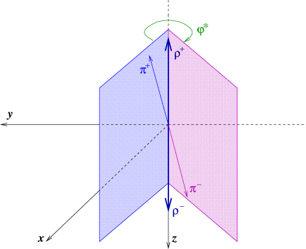
Figure 1: Definition of acoplanarity angle $\varphi^{*}$ in $\rho^{+}\rho^{-}$ pair rest-frame by galf-planes spanned over momenta of each $\rho$ visible decay products. In case of $\tau^{\pm}\to(3\pi)^{\pm}\nu$ four such planes can be defined and thus number of possible acoplanarity angles increases to four (or sixteen if both $\tau^{\pm}$ decay to $3\pi$).

In[3] to control parity of the Higgs boson use of the acoplanarity angle was proposed. Such a definition for $\tau^{\pm}\to\nu\pi^{\pm}\pi^{0}$ rely on directly observable four-momenta, see Fig. 1, only. The distributions were clearly distinct for scalar and mixed parity Higgs, see Fig. 2. To achieve sensitivity the events had to be separated to two groups accordingly to the sign of the product $y_{1}y_{2}$, where

$$y_{1}={E_{\pi^{+}}-E_{\pi^{0}}\over E_{\pi^{+}}+E_{\pi^{0}}},\;\;\;\;y_{2}={E_{\pi^{-}}-E_{\pi^{0}}\over E_{\pi^{-}}+E_{\pi^{0}}}.$$ (6)

All pion energies could be taken in laboratory frame. The reason for $y_{1,2}$ choice were the $\tau$ decay matrix element properties.

1.4 Toward other decay modes

Even though formally distributions of Fig. 2 are one dimensional they require selection with sign of the $y_{1}\cdot y_{2}$ product. In fact, already in the presented above case, minor improvement can be achieved if the statistical analysis of the 3-dimensional distribution over acoplanarity supplemented with $y_{1}$ and $y_{2}$ is studied.

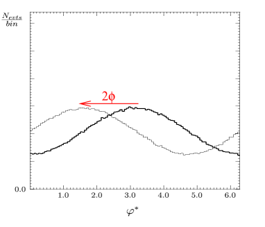
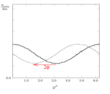
Figure 2: Distribution of acoplanarity angle $\varphi^{*}$ for $\rho^{+}$ and $\rho^{-}$ decay products planes, defined in $\rho^{+}\rho^{-}$ pair rest frame, selection on the sign of $y_{1}\cdot y_{2}$ is used, cases of scalar and mixed scalar-pseudoscalar cases are compared.

This necessity to study multidimensional distribution become even more profound if one turn attention to $\tau$ decays with 3 pions in final state. Then not only one plane can be span over the visible decay products, but four, corresponding to intermediate $a_{1}$ or $\rho$ decays. Indeed, each of such planes provide some sensitivity to Higgs CP, as it can be seen from Fig. 3, taken from Ref.[13]. For each plane pair analogous to eq. (6) selections would need to be studied. Each such distribution is of rather minor sensitivity to CP and also because of correlations, such an approach become challenging from the point of view of statistical analysis.

We have used Machine Learning (ML) techniques available as explained in[12]. Results of Table 1 taken from Ref.[13] are encouraging, they were stable with respect to inclusion of some approximated detector smearing[14] see Table 2. Statistical uncertainties were derived from a bootstrap method. Systematic uncertainty was calculated with the method also described in[14]. We played later, in Ref.[15] with several options of inputs, where so called expert variables, like our acoplanarity angles were used or not. Depending on the ML variants, the performance varied. Sometimes sensitivity was completely absent. In general, structures present in the data, which were of polynomial nature were easy to recognize, but the one related to boosts, especially strongly relativistic boosts, especially when rotatory symmetries had to be identified where challenging for the ML algorithms.

Line content	Channel: $\rho^{\pm}-\rho^{\mp}$	Channel: $a_{1}^{\pm}-\rho^{\mp}$	Channel: $a_{1}^{\pm}-a_{1}^{\mp}$
	$\rho^{\pm}\to\pi^{\pm}\pi^{0}$	$a_{1}^{\pm}\to\rho^{0}\pi^{\pm},\rho^{0}\to\pi^{+}\pi^{-}$	$a_{1}^{\pm}\to\rho^{0}\pi^{\pm},\rho^{0}\to\pi^{+}\pi^{-}$
		$\rho^{0}\to\pi^{+}\pi^{-}$
Fraction of $H\to\tau\tau$	6.5%	4.6%	0.8%
Number of features	24	32	48
True (oracle) classification	0.782	0.782	0.782
ML classification	0.638	0.590	0.557

Table 1: The ML performance for discrimination between scalar ad pseudoscalar Higgs CP state. The 4-momenta of hadronic decay products are used only.

Features				Exact $\pm$ (stat)	Smeared $\pm$ (stat) $\pm$ (syst)	From Ref.[13]
$\phi^{*}$	4-vec	$y_{i}$	$m_{i}$
$a_{1}-\rho$ Decays
✓	✓	✓	✓	$0.6035\pm 0.0005$	$0.5923\pm 0.0005\pm 0.0002$	0.596
✓	✓	✓	-	$0.5965\pm 0.0005$	$0.5889\pm 0.0005\pm 0.0002$	-
✓	✓	-	✓	$0.6037\pm 0.0005$	$0.5933\pm 0.0005\pm 0.0003$	-
-	✓	-	-	$0.5971\pm 0.0005$	$0.5892\pm 0.0005\pm 0.0002$	0.590
✓	✓	-	-	$0.5971\pm 0.0005$	$0.5893\pm 0.0005\pm 0.0002$	0.594
✓	-	✓	✓	$0.5927\pm 0.0005$	$0.5847\pm 0.0005\pm 0.0002$	0.578
✓	-	✓	-	$0.5819\pm 0.0005$	$0.5746\pm 0.0005\pm 0.0002$	0.569
$a_{1}-a_{1}$ Decays
✓	✓	✓	✓	$0.5669\pm 0.0004$	$0.5657\pm 0.0004\pm 0.0001$	0.573
✓	✓	✓	-	$0.5596\pm 0.0004$	$0.5599\pm 0.0004\pm 0.0001$	-
✓	✓	-	✓	$0.5677\pm 0.0004$	$0.5661\pm 0.0004\pm 0.0001$	-
-	✓	-	-	$0.5654\pm 0.0004$	$0.5641\pm 0.0004\pm 0.0001$	0.553
✓	✓	-	-	$0.5623\pm 0.0004$	$0.5615\pm 0.0004\pm 0.0001$	0.573
✓	-	✓	✓	$0.5469\pm 0.0004$	$0.5466\pm 0.0004\pm 0.0001$	0.548
✓	-	✓	-	$0.5369\pm 0.0004$	$0.5374\pm 0.0004\pm 0.0001$	0.536

Table 2: Area Under Curve for Neural Network (NN) trained to separate scalar and pseudoscalar hypotheses with combinations of input features marked with a ✓. Results in the column labeled “Exact” are from NNs trained with exact data. The results in column labeled “Smeared” are from NNs trained with smeared data.

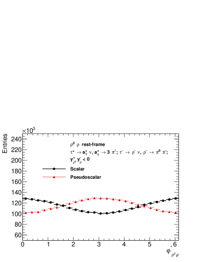
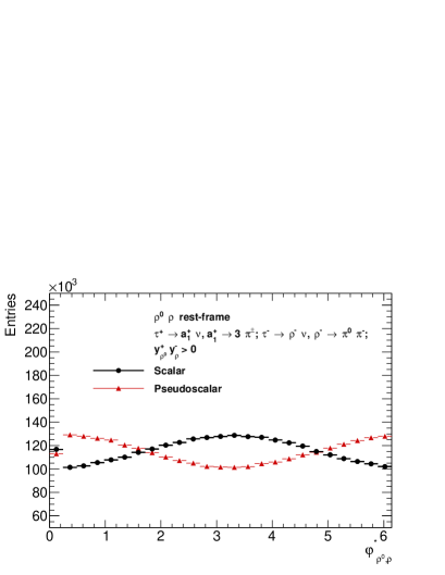
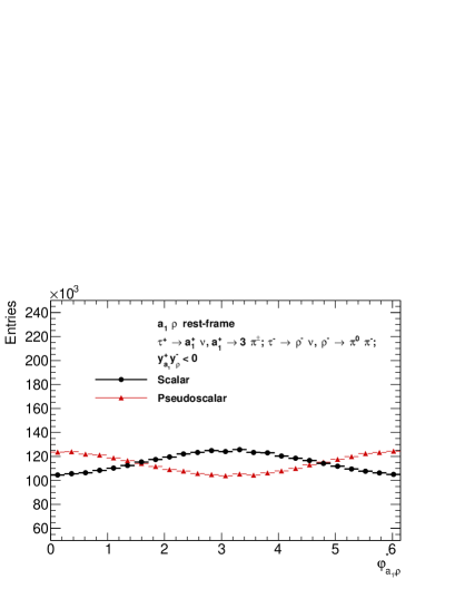
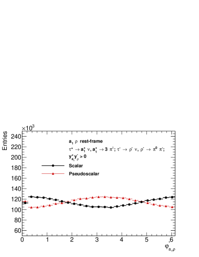
Figure 3: Acoplanarity angles of oriented half decay planes: $\varphi^{*}_{\rho^{0}\rho}$ (top), $\varphi^{*}_{{a_{1}}\rho}$ (bottom), for events grouped by the sign of $y_{\rho^{0}}^{+}y_{\rho}^{-}$ and $y_{a_{1}}^{+}y_{\rho}^{-}$ respectively.

2 Conclusions

In our studies we could observe that ML solutions were helpful for significance evaluation in case of Higgs CP signatures in $H\to\tau\tau$ channel. Massively multi-dimensional signatures could have been controlled. We have identified that features which are related to multi-scale nature of resonance decays of masses ranging from Higgs of 125 GeV to $\rho$ meson of 0.7 GeV wre a challenge for ML. General purpose algorithms such as of Refs.[16, 17, 18] required such adjustment. It was enough to boost and rotate input four momenta to appropriate frames, then use of expert variables was not necessary. On the other hand, solutions, like studied and developed in[19] which are Lorentz group structure savvy may not need such pre-conditioning. ML techniques were useful for phenomenology of Higgs CP in $\tau\tau$ decay channel. For the reversed perspective, the signatures offered good investigation ground for ML algorithms. The case was suitable for such studies, because Matrix Elements are available for event weight calculation. Analytic dependence of weights for Higgs CP dependent part is clear. Studies may be thus of broader than just Higgs CP interest.

On the other hand, even though ML solutions may seem as panacea for all optimization, one should not ignore Optimal Variables approach, which is not only useful to indicate which experimental features are most important for future sensitivity improvements but also provide essential benchmarks. For example, if ML improvements are surprisingly promising, this may indicate that some technical imperfections of Monte Carlo simulations differ e.g. between simulations for signal and background, thus contributing inappropriately to classification.

References

References

- [1] M. Davier, L. Duflot, F. Le Diberder and A. Rouge, Phys. Lett. B 306, 411 (1993).
- [2] S. Schael et al. [ALEPH and DELPHI and L3 and OPAL and SLD Collaborations and LEP Electroweak Working Group and SLD Electroweak Group and SLD Heavy Flavour Group], Phys. Rept. 427 (2006) 257
- [3] G. R. Bower, T. Pierzchala, Z. Was and M. Worek, Phys. Lett. B 543 (2002) 227.
- [4] A. Rouge, Phys. Lett. B619 (2005) 43–49, hep-ex/0505014.
- [5] K. Desch, Z. Was, and M. Worek, Eur. Phys. J. C29 (2003) 491–496, hep-ph/0302046.
- [6] S. Jadach, Z. Was, R. Decker and J. H. Kuhn, Comput. Phys. Commun. 76 (1993) 361.
- [7] N. Davidson, G. Nanava, T. Przedzinski, E. Richter-Was and Z. Was, Comput. Phys. Commun. 183 (2012) 821 doi:10.1016/j.cpc.2011.12.009 [arXiv:1002.0543 [hep-ph]].
- [8] J. H. Kuhn, Phys. Rev. D 52 (1995) 3128 doi:10.1103/PhysRevD.52.3128.
- [9] K. Desch, A. Imhof, Z. Was and M. Worek, Phys. Lett. B 579 (2004) 157.
- [10] V. Cherepanov, E. Richter-Was and Z. Was, SciPost Phys. Proc. 1 (2019) 018 doi:10.21468/SciPostPhysProc.1.018 [arXiv:1811.03969 [hep-ph]].
- [11] S. Berge, W. Bernreuther and S. Kirchner, Phys. Rev. D 92 (2015) 096012.
- [12] I. Goodfellow, Y. Bengio, and A. Courville, Deep learning. MIT Press, Cambridge, MA, 2017.
- [13] R. Jozefowicz, E. Richter-Was and Z. Was, Phys. Rev. D 94 (2016) no.9, 093001 doi:10.1103/PhysRevD.94.093001 [arXiv:1608.02609 [hep-ph]].
- [14] E. Barberio, B. Le, E. Richter-Was, Z. Was, D. Zanzi and J. Zaremba, Phys. Rev. D 96 (2017) 073002,
- [15] K. Lasocha, E. Richter-Was, D. Tracz, Z. Was and P. Winkowska, arXiv:1812.08140.
- [16] T. Chen and C. Guestrin, 1603.02754.
- [17] L. Breiman, Machine Learning 45 (2001), no. 1 5–32.
- [18] A. Bevan, R. Goni, and T. Stevenson, J. Phys. Conf. Ser. 898 (2017), no. 7 072021, 1702.04686.
- [19] M. Erdmann, E. Geiser, Y. Rath and M. Rieger, arXiv:1812.09722 [hep-ex].