Non-adiabatic mass correction for excited states of molecular hydrogen: improvement for the outer-well $H\bar{H}\ ^{1}\Sigma_{\mathrm{g}}^{+}$ term values

Abstract

The mass-correction function is evaluated for selected excited states of the hydrogen molecule within a single-state non-adiabatic treatment. Its qualitative features are studied under the avoided crossing of the $EF$ with the $GK$ state and also for the outer well of the $H\bar{H}$ state. For the $H\bar{H}$ state, a negative mass correction is obtained for the vibrational motion near the outer minimum, which accounts for most of the deviation between experiment and earlier theoretical work.

I Introduction

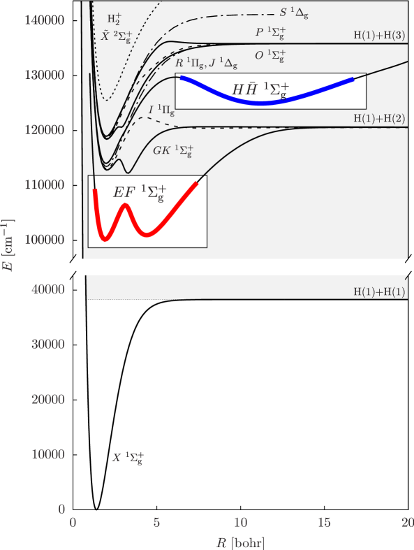
Figure 1: Single-state non-adiabatic treatment for the lower-energy part of the $EF\ ^{1}\Sigma_{\text{g}}^{+}$ electronic state, highlighted in red. Results are obtained within the single-state non-adiabatic framework also for the outer well of the $H\bar{H}\ ^{1}\Sigma_{\text{g}}^{+}$ electronic state, which is highlighted in blue (see also Table 1). The Born–Oppenheimer potential energy curves shown in the figure were compiled from Refs. Wolniewicz (1995a, b); Wolniewicz and Dressler (1994); Wolniewicz et al. (1998); Beyer and Merkt (2016).

This work represents the first steps towards a fully coupled non-adiabatic calculation of the $EF$–$GK$–$H\bar{H}$-etc. singlet-gerade manifold of H₂ including the formerly neglected mass-correction terms which appear in the multi-state, effective non-adiabatic Hamiltonian recently formulated Mátyus and Teufel (2019). Relying on the condition of adiabatic perturbation theory Teufel (2003) that the electronic band must be separated from the rest of the electronic spectrum by a finite gap over the relevant dynamical range, already a single-state treatment delivers insight into the extremely rich non-adiabatic dynamics of electronically excited hydrogen. Motivated by these ideas and after careful inspection of the singlet-gerade manifold, we have selected the lower-energy region of the $EF\ ^{1}\Sigma_{\text{g}}^{+}$ and the outer well of the $H\bar{H}\ ^{1}\Sigma_{\text{g}}^{+}$ state (Figure 1), often labelled with $\bar{H}$, for a single-state non-adiabatic study. After a short summary of the theoretical and computational details, we present the non-adiabatic mass curves and discuss them in relation with earlier theoretical and experimental work.

II Theoretical and computational details

II.1 Summary of the theoretical background

Let us start with the electronic Schrödinger equation,

$$\hat{H}_{\text{el}}\psi_{a}=E_{a}\psi_{a}$$ (1)

including the electronic Hamiltonian (in Hartree atomic units),

$$\hat{H}_{\text{el}} =-\frac{1}{2}\sum_{i=1}^{N_{\text{el}}}\Delta_{\boldsymbol{r}_{i}}+\sum_{i=1}^{N_{\text{el}}}\sum_{j>i}^{N_{\text{el}}}\frac{1}{|\boldsymbol{r}_{i}-\boldsymbol{r}_{j}|}-\sum_{i=1}^{N_{\text{el}}}\sum_{k=1}^{N}\frac{Z_{k}}{|\boldsymbol{r}_{i}-\boldsymbol{R}_{k}|}+\sum_{k=1}^{N}\sum_{l>k}^{N}\frac{Z_{k}Z_{l}}{|\boldsymbol{R}_{k}-\boldsymbol{R}_{l}|}\,$$ (2)

with the $\boldsymbol{r}_{i}$ electronic and the $\boldsymbol{R}_{k}$ nuclear coordinates and $Z_{k}$ nuclear charges. In order to approximate the rovibronic energies of the full, electron-nucleus Schrödinger equation accurately, it is necessary to go beyond the Born–Oppenheimer (BO) approximation. In the present work, we explore the selected states within a single-state non-adiabatic treatment, using the second-order, effective Hamiltonian which had been formulated and reformulated in different contexts Herman and Asgharian (1966); Herman and Ogilvie (1998); Schwenke (2001a); Pachucki and Komasa (2009); Scherrer et al. (2017) and most recently reproduced as a special case of the multi-state effective Hamiltonian Mátyus and Teufel (2019). The single-state Hamiltonian has already been used for the ground electronic state of several diatomic molecules Bunker et al. (1977); Pachucki and Komasa (2008); Mátyus (2018a, b); Przybytek et al. (2017), in an approximate treatment of the water molecule Schwenke (2001b), and in example single-point computations for polyatomics Scherrer et al. (2017) (for a detailed reference list see Ref. Mátyus (2018a)).

The second-order or $\varepsilon^{2}$-, effective Hamiltonian, for the quantum nuclear motion over a selected ‘$a$’ electronic state is

$$\hat{H}^{(2)}_{aa}=\frac{1}{2}\sum_{i=1}^{3N}\sum_{j=1}^{3N}(-\text{i}\varepsilon\partial_{i})(\delta_{ij}-\varepsilon^{2}M_{aa,ij})(-\text{i}\varepsilon\partial_{j})+\varepsilon^{2}U_{a}+E_{a}\;,$$ (3)

where $\varepsilon^{2}$ is the electron-to-nucleus mass ratio, and in particular, for the H₂ molecule in atomic units, it is $\varepsilon^{2}=1/m_{\mathrm{p}}$. $\partial_{i}=\partial/\partial R_{k\alpha}$ with $i=3(k-1)+\alpha$ ($k=1,\ldots,N$, $\alpha=1(x),2(y),3(z)$) is the partial derivative with respect to the nuclear coordinates.

Besides, the nuclear kinetic energy (with constant mass) and the $E_{a}$ electronic energy, $\hat{H}^{(2)}_{aa}$ contains the diagonal Born–Oppenheimer correction (DBOC),

$$\varepsilon^{2}U_{a}=\varepsilon^{2}\frac{1}{2}\sum_{i=1}^{3N}\langle\partial_{i}\psi_{a}|\partial_{i}\psi_{a}\rangle$$ (4)

and the mass correction tensor,

$$\varepsilon^{2}M_{aa,ij} =\varepsilon^{2}2\langle\partial_{j}\psi_{a}|\mathcal{R}_{a}|\partial_{i}\psi_{a}\rangle$$

$$=\varepsilon^{2}2\langle\partial_{j}\psi_{a}|(\hat{H}_{\text{el}}-E_{\text{a}})^{-1}(1-P_{\text{a}})|\partial_{i}\psi_{a}\rangle\ \,,\quad i,j=1,\ldots 3{N}\;,$$ (5)

where the electronic energy, $E_{a}$, and the electronic wave function, $\psi_{a}$, is obtained from solving the electronic Schrödinger equation, Eq. (1). For a better understanding of the numerical results, it will be important to remember the appearance of the reduced resolvent, $\mathcal{R}_{a}=(H_{\text{el}}-E_{a})^{-1}(1-P_{\text{a}})$ with $P_{a}=|\psi_{a}\rangle\langle\psi_{a}|$ in the expression of the mass correction tensor. The ‘effect’ of the outlying electronic states on the quantum nuclear dynamics is accounted for through this reduced resolvent. Also note that the term containing $M_{aa,ij}$ in Eq. (3) is indeed $\mathcal{O}(\varepsilon^{2})$, since we do not assume small nuclear momenta, and hence the action of $\hat{p}_{i}=-\text{i}\varepsilon\partial_{i}$ on the nuclear wave function creates an $\mathcal{O}(1)$ contribution instead of $\mathcal{O}(\varepsilon)$ (for more details, see for example Ref. Mátyus and Teufel (2019)).

The general transformation of the second-order non-adiabatic kinetic energy operator for an $N$-atomic molecule—first term in Eq. (3)—to curvilinear coordinates was worked out in Ref. Mátyus (2018a). The special transformation for a diatomic molecule described with spherical polar coordinates, $(\rho,\Omega)$, which we are using in the present work, had been formulated earlier Herman and Asgharian (1966); Bunker and Moss (1977); Bunker et al. (1977); Pachucki and Komasa (2009). Hence, the effective, non-adiabatic, single-state Schrödinger equation for the hydrogen molecule with $J$ rotational angular momentum quantum number is

$$\left[-\frac{\partial}{\partial\rho}\frac{1}{m_{\mathrm{p}}}\left(1-\frac{(\mathcal{A}_{a})^{\rho}\ _{\rho}}{m_{\mathrm{p}}}\right)\frac{\partial}{\partial\rho}+\frac{J(J+1)}{m_{\mathrm{p}}\ \rho^{2}}\left(1-\frac{(\mathcal{A}_{a})^{\Omega}\ _{\Omega}}{m_{\mathrm{p}}}\right)+\frac{1}{m_{\text{p}}}U_{a}(\rho)+V_{a}(\rho)\right]\phi_{J}(\rho)$$

$$\quad\quad\quad=E_{J}\phi_{J}(\rho)$$ (6)

with the volume element $\text{d}\rho$. The $(\mathcal{A}_{a})^{\rho}\ _{\rho}$ and $(\mathcal{A}_{a})^{\Omega}\ _{\Omega}$ (coordinate-dependent) coefficients originate from the mass-correction tensor, Eq. (5), and the coordinate transformation rule from Cartesian coordinates to curvilinear coordinates (see Ref. Mátyus (2018a, b)). Since, $1/(1+y)\approx 1-y$ for small $y$, we may write $1/m_{\mathrm{p}}(1-a/m_{\mathrm{p}})\approx 1/m_{\mathrm{p}}\cdot 1/(1+a/m_{\mathrm{p}})=1/(m_{\mathrm{p}}+a)$, and in this sense, $(\mathcal{A}_{a})^{\rho}\ _{\rho}$ and $(\mathcal{A}_{a})^{\Omega}\ _{\Omega}$ can be interpreted as correction to the proton mass for the vibrational and rotational motion, or in short, vibrational and rotational mass correction, respectively.

II.2 Computational details

We used the QUANTEN computer program Mátyus and Reiher (2012); Mátyus (2019, 2018a, 2018b) to accurately solve the electronic Schrödinger equation, Eq. (1), for the second, third, and fourth singlet gerade electronic states—$EF$, $GK$, and $H\bar{H}$ ${}^{1}\Sigma_{\text{g}}^{+}$, respectively—of the hydrogen molecule using floating, explicitly correlated Gaussian functions as spatial functions

$$f(\boldsymbol{r};\boldsymbol{A},\boldsymbol{s})=\exp\left[-\frac{1}{2}(\boldsymbol{r}-\boldsymbol{s})^{\text{T}}(\boldsymbol{A}\otimes\boldsymbol{I}_{3})(\boldsymbol{r}-\boldsymbol{s})\right]\;.$$ (7)

The $\boldsymbol{A}\in\mathbb{R}^{2\times 2}$ and $\boldsymbol{s}\in\mathbb{R}^{2\cdot 3}$ parameters were optimized variationally for each basis function at every nuclear configuration, $\boldsymbol{R}_{k}\ (k=1,2)$, over a fine grid of the $\rho=|\boldsymbol{R}_{1}-\boldsymbol{R}_{2}|$ nuclear separation. For the computational details of the wave function derivatives and the mass correction functions in curvilinear coordinates see Refs. Mátyus (2018b, a).

The electronic states we study in this work and the corresponding DBOCs and relativistic corrections have already been computed accurately by Wolniewicz Wolniewicz (1998a) for several proton-proton distances. We have repeated these computations to check the accuracy of the data, and to improve upon it where it was necessary (vide infra). In addition, we have computed the non-adiabatic mass-correction functions in the present work.

The effective nuclear Schrödinger equation for the diatom, Eq. (6), was solved using the discrete variable representation (DVR) Light and Carrington, Jr. (2000) and associated Laguerre polynomials, $L_{n}^{(\alpha)}$ with $\alpha=2$ for the vibrational ($\rho$) degree of freedom. The outer-well $\bar{H}$ states were computed by scaling the DVR points to the $[R_{\text{min}},R_{\text{max}}]=[6,20]$ bohr interval.

III Results and discussion

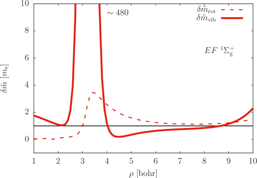
Figure 2: Non-adiabatic mass correction functions to the rotational and the vibrational degrees of freedom, $\delta\tilde{m}_{\text{rot}}$ and $\delta\tilde{m}_{\text{vib}}$, computed for the $EF\ ^{1}\Sigma_{\text{g}}^{+}$ electronic state of the hydrogen molecule Mátyus (2018a, b). (The thin, solid black line indicates the mass of the electron, which together with the proton mass gives the atomic mass.)

The non-adiabatic correction to the vibrational and rotational mass of the proton in the $EF$ and $H\bar{H}$ ${}^{1}\Sigma_{\text{g}}^{+}$ electronic states of H₂ are shown in Figures 2 and 3. These numerical examples highlight qualitative features of the mass-correction functions. The sign and the amplitude of the correction can be understood by remembering that the mass-correction tensor contains the $\mathcal{R}_{\text{a}}$ reduced resolvent, Eq. (5).

The $EF$ state

Concerning the $EF\ ^{1}\Sigma_{\text{g}}^{+}$ state of H₂ below ca. 110 000 cm^-1  (below the $GK$ minima, Figure 1), the effective vibrational mass of the proton becomes gigantic under the avoided crossing with the $GK\ ^{1}\Sigma_{\text{g}}^{+}$ curve. The large correction value, $\delta m_{\text{vib}}^{(EF)}=480\ m_{\mathrm{e}}$ near $R=3$ bohr, which should be compared with the ca. $1836\ m_{\mathrm{e}}$ mass of the proton , indicates that it will be necessary to go beyond the second-order, single-state non-adiabatic treatment to achieve spectroscopic accuracy. For this purpose, one can either consider using higher-order corrections—the third-order correction formulae can be found in Ref. Mátyus and Teufel (2019)—, or including explicit non-adiabatic coupling with the near-lying perturber state(s), in this case $GK$ (and probably other states), and to use the effective non-adiabatic Hamiltonian of Ref. Mátyus and Teufel (2019) for a multi-dimensional electronic subspace. Note that in the single-state treatment only the $EF$ state is projected out from the resolvent, Eq. (5), whereas in a multi-state treatment the full explicitly coupled subspace will be projected out, which will result in smaller corrections from electronic states better separated in energy.

With these observations in mind, we have nevertheless checked the rotation-vibration term values obtained within the second-order, single-state non-adiabatic model. We have found that the $EF$ vibrational term values obtained with the effective masses (Figure 2) were closer to the experimental values than the constant-mass adiabatic description (using either the nuclear mass of the proton or the atomic mass of hydrogen, which is commonly used as an ‘empirical’ means of modeling non-adiabatic effects). The ca. 30–35 cm^-1 root-mean-square deviation of the adiabatic energies from experiment was reduced to 10 cm^-1 when the rigorous non-adiabatic vibrational functions were used instead of the constant (nuclear or atomic) mass. More detailed numerical results will be obtained within a coupled-state non-adiabatic treatment in future work.

The $H\bar{H}$ state

Next, we have studied the $H\bar{H}$ state, for which already a single-state model turns out to be useful for spectroscopic purposes, at least for the outer-well states. The inner well of the $H\bar{H}$ potential energy curve (PEC) gets close to several other PECs, and for this reason a single-state treatment is not appropriate there. At the same time, most of the outer-well state energies (below the barrier) can be accurately computed without considering delocalization to the inner well. This behaviour was pointed out already several times in the literature Wolniewicz (1998a, b); Reinhold et al. (1999); Andersson and Elander (2004); Ross et al. (2006), and we have also checked it for every rovibrational state by solving the rovibrational Schrödinger equation with different $[R_{\text{min}},R_{\text{max}}]$ intervals. In particular, we obtained the (adiabatic) inner-well state energies (below the barrier) with an accuracy better than $0.01$ cm^-1 even if we used the restricted, $[R_{\text{min}},R_{\text{max}}]=[6,20]$ bohr, interval. This behavior was observed either with using constant (e.g., nuclear or atomic) or coordinate-dependent, non-adiabatic masses. The few exceptions (states nearer the top of the barrier which separates the inner and the outer wells) are shown in gray in Table 1.

The experimental term values for the outer-well rotation-vibration states of the $H\bar{H}$ electronic state were first reported in 1997 Reinhold et al. (1997) and also later in 1999 together with an improved theoretical treatment Reinhold et al. (1999); Wolniewicz (1998b). The computations were carried out on an accurate, adiabatic PEC including relativistic corrections and were appended also with an estimate for the quantum electrodynamics (QED) effects Wolniewicz (1998a); Reinhold et al. (1999). The resulting term values were in a ca. 1 cm^-1 (dis)agreement with experiment (of ca. 0.04 cm^-1 uncertainty), which was attributed to the neglect of non-adiabatic effects.

We have repeated the rovibrational computations using the potential energy, diagonal Born–Oppenheimer correction, and relativistic correction curves computed and the QED correction estimated by Wolniewicz Wolniewicz (1998a), but we used the non-adiabatic mass correction functions for the rotational and the vibrational degrees of freedom computed in the present work (Figure 3). We obtained a somewhat better agreement with the experimental results, the 1–1.2 cm^-1 deviation of theory and experiment of Ref. Reinhold et al. (1999) was reduced to 0.3–0.4 cm^-1 (the computed values are larger than the experimental ones).

In order to identify the origin of the remaining discrepancy, we refined the potential energy curve using the QUANTEN program, which resulted in a few tenths of cm^-1 reduction for $R>10$ bohr (the improved electronic energies are deposited in the Supplementary Material som ). Next, we have checked the accuracy of the earlier relativistic corrections and found them to be sufficient for the present purposes. We have also explicitly evaluated the leading-order QED correction (see for example, Eq. (3) of Ref. FeM ), instead of approximating it with the QED correction value of H^- proposed by Wolniewicz Wolniewicz (1998a). For this purpose, we used the one- and two-electron Darwin integrals already available from the relativistic computations Wolniewicz (1998a) and approximated the non-relativistic Bethe-logarithm with $\ln k_{0}\approx 3$ based on its value for the ground state of the hydrogen atom (remember the strong H^-+H⁺ ion-pair character of the outer well and the observation that $\ln k_{0}$ is not very sensitive to the number of electrons Korobov (2018)). We also computed the Araki–Sucher term for the $H\bar{H}$ state in the present work, although it gives an almost negligible contribution at the current level of precision. Based on these computations, the radiative correction curve takes values between 0.27 and 0.29 cm^-1 over the outer well of $H\bar{H}$, and thus we confirm the earlier estimate using the H^- value Wolniewicz (1998a).

As a summary, we collect in Table 1 the best rovibrational term values (‘$T_{\text{nad}}$’ column) and their deviation from experiment (‘nad’ column) resulting from the computations carried out within the present work. Inclusion of the non-adiabatic masses in the rovibrational treatment and further refinement of the potential energy curve reduces the earlier ca. 1–1.5 cm^-1 deviation to ca. 0.1–0.2 cm^-1. The $v\geq 14$ states are shown in grey in the table, because for these states tunneling to the inner well has an important effect on the energy, and an ‘isolated’ outer-well treatment is not sufficient for these states. We also note that the experimental term values for the $v=2$ states with $N=0,1,\ldots,4$ and the $v=2$ and 3 states for $N=5$ are an order-of-magnitude less accurate than for the other states Reinhold et al. (1999, 1997).

In the table, we also compare with experiment the adiabatic energies (a) computed rigorously with the nuclear masses (‘ad${}_{\text{p}}$’ column)—these values are almost identical with the values in Table VI of Ref. Reinhold et al. (1999)—, and (b) with the hydrogenic atomic mass (‘ad${}_{\text{H}}$’ column), which is often used to capture some non-adiabatic effects in the spectrum. In the present case, this atomic-mass model does not perform well, which can be understood by noticing that the rigorous non-adiabatic (vibrational) correction to the nuclear mass is negative over most of the outer well.

Finally, we mention that Andersson and Elander Andersson and Elander (2004), by extending earlier work of Yu and Dressler Yu and Dressler (1994), solved the coupled-state equations, including the coupling of the six lowest-energy ${}^{1}\Sigma_{\text{g}}^{+}$ states, and studied also the outer-well region of $H\bar{H}$. They found that it was necessary to include all six ${}^{1}\Sigma_{\text{g}}^{+}$ states to converge the $\bar{H}$ vibrational energies better than 0.1 cm^-1  whereas the 15th and 16th vibrational states ($v=14$ and 15 in Table 1) changed by 0.12 and 24.11 cm^-1 between the five- and six-state treatment. Although their computed values are off by 10–35 cm^-1 from experiment, probably due to the fact that they used less accurate potential energy curves, their results seem to underline the general observation that the many-state Born–Oppenheimer (BO) expansion converges relatively slowly with respect to the number of electronic states.

IV Summary and conclusions

Due to the slow convergence of the Born–Oppenheimer (BO) expansion with respect to the number of electronic states, it is important to think about the truncation error when one is aiming to compute highly accurate molecular rovibrational (rovibronic) energies. Direct truncation introduces an error of $\mathcal{O}(\varepsilon)$ in the rovibronic energies, where $\varepsilon=(m_{\mathrm{e}}/m_{\text{nuc}})^{1/2}$ is the square root of the electron-to-nucleus mass ratio Mátyus and Teufel (2019); Teufel (2003); Panati et al. (2007). This truncation error can be made lower order in $\varepsilon$ by using adiabatic perturbation theory Teufel (2003); Panati et al. (2007). For an isolated electronic state, the first-order corrections can be made to vanish. The second-order non-adiabatic effective Hamiltonian, used in the present work, reproduces eigenvalues of the full electron-nucleus Hamiltonian with an error of $\mathcal{O}(\varepsilon^{3})$, but it contains corrections both to the potential energy as well as to the kinetic energy of the atomic nuclei Mátyus and Teufel (2019), which gives rise to effective coordinate-dependent masses to the different types of motions.

In particular, we have found a non-trivial, negative mass-correction to the vibrational mass of the proton in the outer well of the $H\bar{H}\ ^{1}\Sigma_{\text{g}}^{+}$ electronic state. This negative value, i.e., an effective vibrational mass smaller than the nuclear mass, is dominated by the interaction with the H(1)+H(2) dissociation channel to which $H\bar{H}$ gets close near its outer minimum. Of course, the precise value of the mass correction is the result of an interplay of the interaction of the nuclear dynamics on $H\bar{H}$ with all the other (discrete and continuous) electronic states. It is interesting to note that, whereas the vibrational mass shows this special behaviour for $H\bar{H}$, the non-adiabatic value of the rotational mass remains close to the atomic mass of the hydrogen (proton plus electron, see Figure 3). Due to these properties, $H\bar{H}$ makes a counter-example to the simple, empirical recipe according to which small non-adiabatic effects can be ‘approximately modeled’ by using (near) the atomic mass value for vibrations and the nuclear mass for rotations Polyansky and Tennyson (1999); Diniz et al. (2013); Mátyus et al. (2014). In the case of the outer well of $H\bar{H}$, the vibrational mass is better approximated by the nuclear mass, while the rotational mass equals the atomic mass to a good approximation. Using the rigorous non-adiabatic, mass-correction functions computed in the present work, the non-adiabatic rovibrational energies are ca. 1 cm^-1 (2 cm^-1) larger than the energies obtained using the nuclear (atomic) mass. This, together with the relativistic and radiative corrections as well as with a minor, 0.1–0.2 cm^-1 improvement for the outer-well electronic energies, allows us to achieve a 0.1–0.2 cm^-1 agreement, an order of magnitude better than earlier theory, with experiment Reinhold et al. (1997, 1999).

All in all, we have demonstrated that small, non-adiabatic corrections in the (high-resolution) spectrum can be efficiently described using the effective non-adiabatic Hamiltonian which accounts for the truncation error in the electronic space perturbatively. For the particular case of the outer well of the $H\bar{H}\ ^{1}\Sigma_{\text{g}}^{+}$ electronic state, the discrepancy of earlier theoretical work with experiment can be accounted for by a non-trivial decrease in the effective, non-adiabatic vibrational mass of the protons as they pass along near-lying electronic states.

Acknowledgement

We acknowledge financial support from a PROMYS Grant (no. IZ11Z0_166525) of the Swiss National Science Foundation. DF thanks a doctoral scholarship from the New National Excellence Program of the Ministry of Human Capacities of Hungary (ÚNKP-18-3-II-ELTE-133). EM thanks ETH Zürich for a visiting professorship during 2019 and the Laboratory of Physical Chemistry for their hospitality, where part of this work has been completed.

Table 1: Term values and deviation from experiment, in cm^-1, for the outer-well rovibrational states of the $H\bar{H}\ ^{1}\Sigma_{\text{g}}^{+}$ electronic state of the hydrogen molecule.

		$J=0$					$J=1$					$J=2$
			$T_{\text{obs}}-T_{\text{calc}}$${}^{\text{a}}$					$T_{\text{obs}}-T_{\text{calc}}$${}^{\text{a}}$					$T_{\text{obs}}-T_{\text{calc}}$${}^{\text{a}}$
$v$		$T_{\text{nad}}$${}^{\text{b}}$	nad${}^{\text{c}}$	ad${}_{\text{H}}$${}^{\text{d}}$	ad${}_{\text{p}}$${}^{\text{e}}$		$T_{\text{nad}}$${}^{\text{b}}$	nad${}^{\text{c}}$	ad${}_{\text{H}}$${}^{\text{d}}$	ad${}_{\text{p}}$${}^{\text{e}}$		$T_{\text{nad}}$${}^{\text{b}}$	nad${}^{\text{c}}$	ad${}_{\text{H}}$${}^{\text{d}}$	ad${}_{\text{p}}$${}^{\text{e}}$
0		122883.4		n.a.f			122885.3		n.a.f			122889.1		n.a.f
1		123234.5		n.a.f			123236.4		n.a.f			123240.2		n.a.f
2		123575.8	$0.1$g	$1.1$g	$0.9$g		123577.7	$0.0$g	$1.0$g	$0.8$g		123581.5	$0.2$g	$1.1$g	$0.9$g
3		123907.5	$-0.2$	$1.1$	$0.8$		123909.4	$-0.2$	$1.1$	$0.8$		123913.3	$-0.2$	$1.1$	$0.8$
4		124229.9	$-0.2$	$1.3$	$0.9$		124231.8	$-0.2$	$1.3$	$0.9$		124235.7	$-0.3$	$1.2$	$0.8$
5		124543.0	$-0.3$	$1.4$	$0.9$		124544.9	$-0.3$	$1.4$	$0.9$		124548.8	$-0.3$	$1.4$	$0.9$
6		124847.2	$-0.2$	$1.6$	$1.1$		124849.1	$-0.2$	$1.6$	$1.0$		124853.0	$-0.2$	$1.6$	$1.0$
7		125142.5	$-0.2$	$1.7$	$1.1$		125144.5	$-0.2$	$1.7$	$1.1$		125148.4	$-0.2$	$1.7$	$1.1$
8		125429.3	$-0.2$	$1.8$	$1.2$		125431.3	$-0.1$	$1.8$	$1.2$		125435.1	$-0.2$	$1.8$	$1.1$
9		125707.6	$-0.1$	$1.9$	$1.2$		125709.6	$-0.1$	$2.0$	$1.3$		125713.5	$-0.1$	$1.9$	$1.2$
10		125977.6	$-0.1$	$1.9$	$1.2$		125979.5	$-0.1$	$2.0$	$1.2$		125983.4	$-0.1$	$1.9$	$1.2$
11		126239.1	$-0.1$	$1.9$	$1.1$		126241.1	$-0.1$	$2.0$	$1.2$		126245.0	$-0.2$	$1.9$	$1.1$
12		126492.4	$-0.2$	$1.9$	$1.1$		126494.4	$-0.2$	$1.9$	$1.0$		126498.3	$-0.2$	$1.9$	$1.0$
13${}^{\text{h}}$		126737.1	$-0.2$	$1.8$	$0.9$		126739.1	$-0.2$	$1.8$	$0.9$		126743.1	$-0.3$	$1.8$	$0.9$
14${}^{\text{h}}$		126972.9	$-0.5$	$1.5$	$0.6$		126975.0	$-0.5$	$1.5$	$0.6$		126979.1	$-0.6$	$1.4$	$0.5$
15${}^{\text{h}}$		127199.3	$-1.8$	$0.2$	$-0.8$		127201.4	$-1.7$	$0.3$	$-0.7$		127205.6	$-1.5$	$0.4$	$-0.5$
		$J=3$					$J=4$					$J=5$
			$T_{\text{obs}}-T_{\text{calc}}$${}^{\text{a}}$					$T_{\text{obs}}-T_{\text{calc}}$${}^{\text{a}}$					$T_{\text{obs}}-T_{\text{calc}}$${}^{\text{a}}$
$v$		$T_{\text{nad}}$${}^{\text{b}}$	nad${}^{\text{c}}$	ad${}_{\text{H}}$${}^{\text{d}}$	ad${}_{\text{p}}$${}^{\text{e}}$		$T_{\text{nad}}$${}^{\text{b}}$	nad${}^{\text{c}}$	ad${}_{\text{H}}$${}^{\text{d}}$	ad${}_{\text{p}}$${}^{\text{e}}$		$T_{\text{nad}}$${}^{\text{b}}$	nad${}^{\text{c}}$	ad${}_{\text{H}}$${}^{\text{d}}$	ad${}_{\text{p}}$${}^{\text{e}}$
0		122894.9		n.a.f			122902.5		n.a.f			122912.0		n.a.f
1		123246.0		n.a.f			123253.6		n.a.f			123263.2		n.a.f
2		123587.3	$0.0$g	$1.0$g	$0.8$g		123595.0	$0.4$g	$1.4$g	$1.2$g		123604.6	$-0.3$g	$0.7$g	$0.5$g
3		123919.1	$-0.2$	$1.0$	$0.7$		123926.8	$-0.2$	$1.1$	$0.7$		123936.4	$0.0$g	$1.3$g	$0.9$g
4		124241.5	$-0.2$	$1.2$	$0.9$		124249.2	$-0.3$	$1.2$	$0.8$		124258.8	$-0.2$	$1.3$	$0.9$
5		124554.6	$-0.2$	$1.4$	$1.0$		124562.3	$-0.3$	$1.4$	$0.9$		124572.0	$-0.2$	$1.4$	$0.9$
6		124858.8	$-0.2$	$1.6$	$1.1$		124866.5	$-0.2$	$1.6$	$1.0$		124876.2	$-0.2$	$1.6$	$1.0$
7		125154.2	$-0.1$	$1.8$	$1.2$		125161.9	$-0.2$	$1.7$	$1.1$		125171.6	$-0.2$	$1.7$	$1.1$
8		125441.0	$-0.2$	$1.8$	$1.2$		125448.7	$-0.2$	$1.8$	$1.1$		125458.4	$-0.2$	$1.8$	$1.2$
9		125719.3	$-0.1$	$1.9$	$1.2$		125727.0	$-0.1$	$1.9$	$1.2$		125736.7	$-0.1$	$1.9$	$1.2$
10		125989.3	$-0.1$	$2.0$	$1.2$		125997.0	$-0.1$	$1.9$	$1.2$		126006.8	$-0.1$	$1.9$	$1.2$
11		126250.9	$-0.1$	$2.0$	$1.2$		126258.7	$-0.2$	$1.9$	$1.1$		126268.5	$-0.1$	$1.9$	$1.1$
12		126504.2	$-0.2$	$1.9$	$1.0$		126512.1	$-0.2$	$1.9$	$1.0$		126522.0	$-0.2$	$1.9$	$1.0$
13${}^{\text{h}}$		126749.1	$-0.3$	$1.8$	$0.9$		126757.1	$-0.3$	$1.8$	$0.9$		126767.1	$-0.3$	$1.8$	$0.9$
14${}^{\text{h}}$		126985.2	$-0.4$	$1.6$	$0.7$		126993.4	$-0.6$	$1.4$	$0.5$		127003.6	$-0.4$	$1.7$	$0.7$
15${}^{\text{h}}$		127211.9	$-1.3$	$0.7$	$-0.3$		127220.4	$-0.9$	$1.1$	$0.1$		127230.8

(Please find the footnotes on the next page)

Footnotes to Table 1

${}^{\text{a}}$ Deviation of experiment and theory. The $T_{\text{obs}}$ experimental term values were taken from Refs. Reinhold et al. (1997, 1999).

${}^{\text{b}}$ Calculated term value, $T_{\text{nad}}=E_{\text{nad}}-E_{0}$, referenced to the ground-state energy, $E_{0}$ Wang and Yan (2018); Puchalski et al. (2018). $E_{\text{nad}}$ was obtained by solving Eq. (6) with the rigorous non-adiabatic masses computed in the present work (Figure 3) and using the relativistic and diagonal Born–Oppenheimer corrections of Ref. Wolniewicz (1998a, b), as well as the radiative corrections and an improved PEC computed in this work.

${}^{\text{c}}$ $T_{\text{calc}}=T_{\text{nad}}$.

${}^{\text{d}}$ $T_{\text{calc}}=T_{\text{ad}_{\text{H}}}=E_{\text{ad}_{\text{H}}}-E_{0}$, where $E_{\text{ad}_{\text{H}}}$ was obtained as $E_{\text{nad}}$ but using the constant, atomic mass of hydrogen for $m_{\text{p}}$ and approximating the mass-correction functions by zero.

${}^{\text{e}}$ $T_{\text{calc}}=T_{\text{ad}_{\text{p}}}=E_{\text{ad}_{\text{p}}}-E_{0}$, where $E_{\text{ad}_{\text{p}}}$ was obtained as $E_{\text{ad}_{\text{H}}}$ but using the constant, nuclear mass of the proton for $m_{\text{p}}$.

${}^{\text{f}}$ Experimental data not available.

${}^{\text{g}}$ Note that the experimental uncertainty is an order-of-magnitude larger for these term values than for the others.

${}^{\text{h}}$ Neglect of delocalization to the inner well introduces an at least 0.1 cm^-1 error in the computed energy.

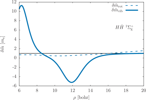
Figure 3: Non-adiabatic mass correction functions to the rotational and the vibrational degrees of freedom, $\delta\tilde{m}_{\text{rot}}$ and $\delta\tilde{m}_{\text{vib}}$, computed for the $H\bar{H}\ ^{1}\Sigma_{\text{g}}^{+}$ electronic state of the hydrogen molecule Mátyus (2018a, b). (The thin, solid black line indicates the mass of the electron, which together with the proton mass gives the atomic mass.)

References

- Mátyus and Teufel (2019) E. Mátyus and S. Teufel, J. Chem. Phys. 151, 014113 (2019).
- Teufel (2003) S. Teufel, Adiabatic Perturbation Theory in Quantum Dynamics, Lecture Notes in Mathematics (Springer-Verlag, Berlin, Heidelberg, New York, 2003).
- Herman and Asgharian (1966) R. M. Herman and A. Asgharian, J. Mol. Spectrosc. 19, 305 (1966).
- Herman and Ogilvie (1998) R. M. Herman and J. F. Ogilvie, Adv. Chem. Phys. 103, 187 (1998).
- Schwenke (2001a) D. W. Schwenke, J. Chem. Phys. 114, 1693 (2001a).
- Pachucki and Komasa (2009) K. Pachucki and J. Komasa, J. Chem. Phys. 130, 164113 (2009).
- Scherrer et al. (2017) A. Scherrer, F. Agostini, D. Sebastiani, E. K. U. Gross, and R. Vuilleumier, Phys. Rev. X 7, 031035 (2017).
- Bunker et al. (1977) P. R. Bunker, C. J. McLarnon, and R. E. Moss, Mol. Phys. 33, 425 (1977).
- Pachucki and Komasa (2008) K. Pachucki and J. Komasa, J. Chem. Phys. 129, 034102 (2008).
- Mátyus (2018a) E. Mátyus, J. Chem. Phys. 149, 194111 (2018a).
- Mátyus (2018b) E. Mátyus, J. Chem. Phys. 149, 194112 (2018b).
- Przybytek et al. (2017) M. Przybytek, W. Cencek, B. Jeziorski, and K. Szalewicz, Phys. Rev. Lett. 119, 123401 (2017).
- Schwenke (2001b) D. W. Schwenke, J. Phys. Chem. A 105, 2352 (2001b).
- Bunker and Moss (1977) P. R. Bunker and R. E. Moss, Mol. Phys. 33, 417 (1977).
- Mátyus and Reiher (2012) E. Mátyus and M. Reiher, J. Chem. Phys. 137, 024104 (2012).
- Mátyus (2019) E. Mátyus, Mol. Phys. 117, 590 (2019).
- Wolniewicz (1998a) L. Wolniewicz, J. Chem. Phys. 109, 2254 (1998a).
- Light and Carrington, Jr. (2000) J. C. Light and T. Carrington, Jr., Adv. Chem. Phys. 114, 263 (2000).
- Wolniewicz (1998b) L. Wolniewicz, J. Chem. Phys. 108, 1499 (1998b).
- Reinhold et al. (1999) E. Reinhold, W. Hogervorst, W. Ubachs, and L. Wolniewicz, Phys. Rev. A 60, 1258 (1999).
- Andersson and Elander (2004) S. Andersson and N. Elander, Phys. Rev. A 69, 052507 (2004).
- Ross et al. (2006) S. C. Ross, T. Yoshinari, Y. Ogi, and K. Tsukiyama, J. Chem. Phys. 125, 133205 (2006).
- Reinhold et al. (1997) E. Reinhold, W. Hogervorst, and W. Ubachs, Phys. Rev. Lett. 78, 2543 (1997).
- (24) The supplementary material contains the improved electronic energies for the outer well of the electronic state obtained in the present work.
- (25) D. Ferenc and E. Mátyus, Precise computation of rovibronic resonances of molecular hydrogen: inner-well rotational states. arXiv:1904.08609.
- Korobov (2018) V. I. Korobov, Mol. Phys. 116, 93 (2018).
- Yu and Dressler (1994) S. Yu and K. Dressler, J. Chem. Phys. 101, 7692 (1994).
- Panati et al. (2007) G. Panati, H. Spohn, and S. Teufel, ESAIM: Mathematical Modelling and Numerical Analysis 41, 297 (2007).
- Polyansky and Tennyson (1999) O. L. Polyansky and J. Tennyson, J. Chem. Phys. 110, 5056 (1999).
- Diniz et al. (2013) L. G. Diniz, J. R. Mohallem, A. Alijah, M. Pavanello, L. Adamowicz, O. L. Polyansky, and J. Tennyson, Phys. Rev. A 88, 032506 (2013).
- Mátyus et al. (2014) E. Mátyus, T. Szidarovszky, and A. G. Császár, J. Chem. Phys. 141, 154111 (2014).
- Wang and Yan (2018) L. M. Wang and Z.-C. Yan, Phys. Rev. A 97, 060501(R) (2018).
- Puchalski et al. (2018) M. Puchalski, A. Spyszkiewicz, J. Komasa, and K. Pachucki, Phys. Rev. Lett. 121, 073001 (2018).
- Wolniewicz (1995a) L. Wolniewicz, J. Mol. Spectrosc. 174, 132 (1995a).
- Wolniewicz (1995b) L. Wolniewicz, J. Mol. Spectrosc. 169, 329 (1995b).
- Wolniewicz and Dressler (1994) L. Wolniewicz and K. Dressler, J. Chem. Phys. 100, 444 (1994).
- Wolniewicz et al. (1998) L. Wolniewicz, I. Simbotin, and A. Dalgarno, Astrophys. J. Suppl. Ser. 115, 293 (1998).
- Beyer and Merkt (2016) M. Beyer and F. Merkt, J. Mol. Spectrosc. 330, 147 (2016).