Consensus-based Interpretable Deep Neural Networks with Application to Mortality Prediction

Abstract

Deep neural networks have achieved remarkable success in various challenging tasks. However, the black-box nature of such networks is not acceptable to critical applications, such as healthcare. In particular, the existence of adversarial examples and their overgeneralization to irrelevant, out-of-distribution inputs with high confidence makes it difficult, if not impossible, to explain decisions by such networks. In this paper, we analyze the underlying mechanism of generalization of deep neural networks and propose an ($n$, $k$) consensus algorithm which is insensitive to adversarial examples and can reliably reject out-of-distribution samples. Furthermore, the consensus algorithm is able to improve classification accuracy by using multiple trained deep neural networks. To handle the complexity of deep neural networks, we cluster linear approximations of individual models and identify highly correlated clusters among different models to capture feature importance robustly, resulting in improved interpretability. Motivated by the importance of building accurate and interpretable prediction models for healthcare, our experimental results on an ICU dataset show the effectiveness of our algorithm in enhancing both the prediction accuracy and the interpretability of deep neural network models on one-year patient mortality prediction. In particular, while the proposed method maintains similar interpretability as conventional shallow models such as logistic regression, it improves the prediction accuracy significantly.

Introduction

Cardiovascular diseases (CVDs) cause severe economic and healthcare related burdens not only in the United States but worldwide [Benjamin et al., 2018]. Acute myocardial infarction (AMI) is a type of CVD which is defined as “myocardial necrosis in a clinical setting consistent with myocardial ischemia”, or heart attack in simple words [Members et al., 2012]. AMI is the leading cause of death worldwide [Reed, Rossi, and Cannon, 2017]. Identifying risky patients in Intensive Care Unit (ICU) and preparing for their health needs are crucial to health planners and health providers [DeSalvo et al., 2006]. This enables them to appropriately manage AMI and employ timely interventions to reduce mortality from CVD [McNamara et al., 2016]. These facts motivate recent efforts on building mortality prediction models for ICU patients with AMI  [Kawaguchi et al., 2018]. Electronic health records (EHRs) with rich data of patient encounters present unprecedented opportunities for critical clinical applications such as outcome prediction [Shickel et al., 2017]. However, medical data are typically heterogeneous and building machine learning models using this type of data is more challenging than using homogeneous data like images. The necessity of dealing with heterogeneous data is not limited to medical applications, but it is shared among many other applications of machine learning [L’heureux et al., 2017].

Figure 1: The workflow of the study (Icons made by https://www.flaticon.com)

Unlike traditional machine learning approaches, deep learning methods do not require feature engineering [Steele et al., 2018]. Such networks have demonstrated significant successes in many challenging tasks and applications [LeCun, Bengio, and Hinton, 2015]. Even though they have been employed in numerous real-world applications to enhance the user experience, their adoption in healthcare and clinical practice has been slow. Among the inherent difficulties, the complexity of these models remains a huge challenge [Ahmad, Eckert, and Teredesai, 2018] as it is not clear how they arrive at their predictions [Zhang, Nian Wu, and Zhu, 2018]. In medical practice, it is unacceptable to only rely on predictions made by a black-box model to guide decision-making for patients. Ideally, medical professionals should be able to point out the conditions under which the model works. Any incorrect prediction such as erroneous diagnosis may lead to serious medical errors, which is currently the third leading cause of death in the United States [Makary and Daniel, 2016]. This issue has been raised and the necessity of interpretable deep learning models has been identified [Adadi and Berrada, 2018]. However, it is not clear how to improve the interpretability and at the same time retain the accuracy of deep neural networks. Deep neural networks have improved application performance by capturing complex latent relationships among input variables. To make the matter worse, these models are typically overparameterized, i.e., they have more parameters than the number of training samples [Zhang et al., 2016]. Overparametrization simplifies the optimization problem for finding good solutions [Allen-Zhu, Li, and Liang, 2018]; however, the resulting solutions are even more complex and more difficult to interpret. Consequently, interpretability enhancement techniques would be difficult without handling the complexity of deep neural networks.

Recognizing that commonly-used activation functions (ReLU, sigmoid, tanh, and so on) are piece-wise linear or can be well approximated by a piece-wise linear function, such neural networks partition the input space into (approximately) linear regions. In addition, gradient-based optimization results in similar linear regions for similar inputs as their gradient tends to be similar. By clustering the linear regions, we can reduce the number of distinctive linear regions and at the same time improve robustness. To further improve the performance, we train multiple models and use consensus among the models to reduce their sensitivity to adversarial examples with small perturbations and also reduce overgeneralization to irrelevant inputs of individual models. We demonstrate the effectiveness of deep neural network models and the proposed algorithms on one-year mortality prediction in patients diagnosed with AMI or post myocardial infarction (PMI) in MIMIC-III database. The workflow of this study is depicted in Fig. 1. Furthermore, the experimental results show that the proposed method improves the performance as well as the interpretability.

The paper is organized as follows. In the next section, we present generalization and overgeneralization in the context of deep neural networks and the proposed deep ($n$, $k$) consensus-based classification algorithm. After that, we describe a consensus-based interpretability method. Then, we illustrate the effectiveness of the proposed algorithms in enhancing one-year mortality predictions via experiments. Finally, we review recent studies that are closely related to our work and conclude the paper with a brief summary and plan for future work.

Generalization and Overgeneralization in Deep Neural Networks

Fundamentally, a neural network approximates the underlying but unknown function using $f(x;\theta)$, where $x$ is the input, and $\theta$ is a vector that includes all the parameters (weights and biases). Given a deep learning model and a training dataset, there are two fundamental problems to be solved: optimization and generalization. The optimization problem deals with finding the parameters $\theta$ by minimizing a loss function on the training set. Overparametrization [Neyshabur et al., 2018] in deep neural networks makes the problem easier to solve by increasing the number of good solutions exponentially [Wu, Zhu, and Weinan, 2017].

Since there are numerous good solutions, understanding their differences and commonalities is essential to developing more effective multiple-model based methods. Toward a systematic understanding of deep neural network models in the input space, one must consider the behavior of these models in case of typical, irrelevant and adversarial inputs (the inputs that are “computed” intentionally to degrade the system performance) [Goodfellow, Shlens, and Szegedy, 2014]. Previously, we study the response of multiple deep network models to irrelevant images systematically and show that such models behave almost randomly to irrelevant inputs. Furthermore, we study the response of the models on adversarial examples generated by perturbing the inputs with one of the models using fast sign algorithm [Goodfellow, Shlens, and Szegedy, 2014]. Please see the previous version of the work for detailed results.

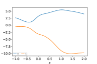
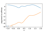
Figure 2: Outputs from the penultimate layer for model 1, 2, 3, 4 and 5 respectively centered at a training sample, along the direction to another sample in the same class.

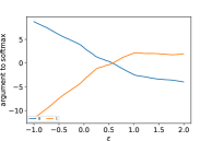
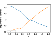
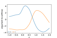
Figure 3: Outputs from the penultimate layer for model 1, 2, 3, 4 and 5 respectively centered at a training sample, along the direction to another sample in the other class.

Deep (n, k) Consensus Algorithm

As all the models classify training samples accurately, they generate similar linear regions and should behave similarly at training samples. In Fig. 2, the model generalizes perfectly along the path of the same class even though they differ in details. We find this is a representative behavior, main reason why multiple DNN models mostly agree with each other to meaningful inputs and can filter out adversarial and irrelevant samples. While individual approximations are sensitive to adversarial examples, consensus can be used to capture the underlying common structures in training data, not accidental features. Similar to Fig. 2, Fig. 3 shows that along the path to other class, all models behave similarly in that the decision boundaries occur around 0.5 and there is no significant oscillation between class 0 and 1 samples. Therefore, consensus between the models makes sense.

We propose to use consensus among different models to differentiate extrinsically classified samples from intrinsically/consistently classified samples (CCS). Samples are considered to be consistently classified if they are classified by multiple models with a high probability in the same class. In contrast, extrinsic factors such as randomness of weight initialization or oversensitiveness to accidental features are responsible for the classification of extrinsic samples. As such random factors cannot happen consistently in multiple models, we can reduce them exponentially by using more models.

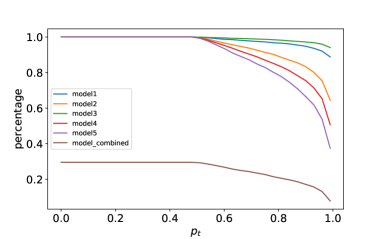
Figure 4: (to be viewed in color) Percentage of classified overgeneralized samples with (5,5) consensus. The samples are out-of-distribution inputs for the one-year patient mortality prediction dataset.

To tolerate accidental oversensitiveness of a small number of models, we propose deep ($n$, $k$) consensus algorithm, which is given in Algorithm 1. Note that $P_{min}$ is a vector with one value for each class as it is computed class-wise. Essentially, the algorithm requires consensus among $k$ out of $n$ trained models in order for a sample to be classified; $p_{t}$, a threshold parameter, is used to decide if the prediction probability of a model is sufficiently high.

Algorithm 1 Deep (n, k) consensus-based classification

0:  Trained models $M_{1}$, $M_{2}$,…, $M_{n}$, input $x$, and parameter $p_{t}$

1:  Apply each of the models to classify $x$ and retain the probabilities for each class as $P_{M_{i}}$

2:  Compute $P_{min}$ by finding the class-wise minimal among top $k$ $P_{M_{i}}$

3:  If $max(P_{min})>p_{t}$,

4:      Classify $x$ as the class with maximum $max(P_{min})$

5:  Else

6:      Reject to classify $x$ (mark it as ambiguous)

7:  Endif

To illustrate the effectiveness of the proposed algorithm, Fig. 4 shows the results on the irrelevant samples, generated using randomized values. Majority of the irrelevant samples are rejected using a (5, 5) consensus algorithm as shown in Fig. 4; note that a (5,4) algorithm would also be effective even though it could not reject the ones where four models agree accidentally.

As a whole, the deep network models generalize in a similar way for the intrinsic features. Even though all the models behave consistently for the samples that are supported by the training set, however their behavior can differ in terms of the exact direction that leads to adversarial examples. Therefore, the consensus among the models should also be able to reduce adversarial examples. We have conducted systematic experiments to illustrate that, where after generating adversarial examples using one model, most of the other models are able to reject them (see previous version of the work).

Note that the proposed algorithm is different from ensemble methods [Ju, Bibaut, and van der Laan, 2017], which are used to improve the performance of multiple models via voting. Similarly, in applications (such as data mining) where a set of samples need to be classified by possibly multiple classifiers at the same time, correlations between different classes can be utilized to create multiple labels for similar objects by maximizing agreements among the assigned labels to the objects (e.g., Xie et al. [2013]). Note that these methods can not recognize and reject adversarial and out-of-distribution samples while our algorithm is designed to handle those samples via inherent consensus of the multiple deep neural network models. In addition, the proposed consensus-based algorithm is not trying to force or maximize the consensus among the models for the classification task, rather because the consensus exists naturally in deep networks for the samples they can generalize.

A Consensus-based Interpretability Method

With a robust way to handle irrelevant and adversarial inputs, we propose a novel method to interpret decisions by trained deep neural networks, based on that such networks behave linearly locally and linear regions form clusters due to weight symmetry.

The linear approximation, reveals rich deep neural network model behavior in the neighborhood of a sample. Interesting characteristics of the model can be uncovered by walking along certain directions from the sample. For example, adversarial examples are clearly evident along the direction shown in Fig. 3, where the classification changes quickly outside $\epsilon=0$ (where the given training sample is). On the other hand, Fig. 2 shows robust classification along this particular direction.

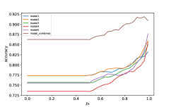
(a)

(b)

(c)

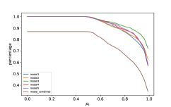
(d)

Figure 5: (to be viewed in color) Change of accuracy and percentage of CCS samples with deep ($n$, $k$) consensus on the one-year patient mortality prediction dataset. (a) shows the increase of intrinsic accuracy while (5,5) consensus. (b) shows the percentage of CCS samples while (5,5) consensus. (c) shows the increase of intrinsic accuracy while (5,4) consensus. (d) shows the percentage of CCS samples while (5,4) consensus.

More formally, under the assumption that the last layer in a neural network is a softmax layer, we can analyze the outputs from the penultimate layer (i.e., the layer before the softmax layer). Using the notations introduced earlier, the outputs can be written as the following:

$$\mathbf{O}=f(\mathbf{x},\theta),$$ (1)

where $\mathbf{O}$ is the vector-valued function. Since the model is locally close to linear, if we perturb an input (e.g., $\mathbf{x}_{0}$) by a small value $\Delta x$ (i.e., $\mathbf{x}=\mathbf{x}_{0}+\Delta x$), then the Equation 1 can be approximated using the first order Taylor expansion around input $\mathbf{x}_{0}$.

$$\mathbf{O}\approx f(\mathbf{x}_{0},\theta)+\mathbf{J}\Delta x$$ (2)

Here, $\mathbf{J}$ is the Jacobian matrix of function $\mathbf{O}$, defined as $J_{i,j}=\frac{\partial O_{i}}{\partial x_{j}}$. Note that the gradient or the Jacobian matrix, in general, has been used in a number of methods to enhance interpretability (e.g., Simonyan, Vedaldi, and Zisserman [2013]; Sundararajan, Taly, and Yan [2017]).

However, the Jacobian matrix only reflects the changes for each output individually. As classification is inherently a discriminative task, the difference between the two largest outputs is locally important. In the binary case, we can write the difference of the two outputs as:

$$o_{2}-o_{1}=f_{2}(\mathbf{x}_{0},\theta)-f_{1}(\mathbf{x}_{0},\theta)+(\mathbf{J}_{1,:}-\mathbf{J}_{0,:})\Delta x,$$ (3)

where $\mathbf{J}_{0,:}$ and $\mathbf{J}_{1,:}$ are the first and second row of $\mathbf{J}$. In general, for multiple class cases, we need to analyze the difference between the top two outputs locally. For example, we can focus on the difference between the top 2 classes, even though there are 10 classes in case of MNIST dataset [Lecun et al., 1998]. In general, we can apply pairwise difference analysis; however, most pairs will be irrelevant locally. The differences between bottom classes are likely due to noisy.

The Jacobian difference vector essentially determines the contributions of changes in the features, i.e., the feature importance locally. This allows us to explain why the deep neural network model behaves in a particular way in the neighborhood of a sample. Note that the first part of Equation 3, i.e., $f_{2}(\mathbf{x}_{0},\theta)-f_{1}(\mathbf{x}_{0},\theta)$ is important to achieve high accuracy. However, the local Jacobian matrices, while important, are not robust. To increase the robustness of interpretation and at the same time reduce the complexity, we propose to cluster the difference vectors of Jacobian matrices.

The Jacobian difference vectors can be clustered using K-means or any other clustering algorithm. In this paper, we identify consistent clusters using the correlation coefficients of the Jacobian difference vectors of the training samples. To create a cluster, we first identify the pair that has the highest correlation. Then, we expand the cluster by adding the sample with the highest correlation with all the samples in the cluster already. This can be done efficiently by computing the minimum correlations to the ones in the cluster already for each remaining sample and then choosing the one with the maximum. We add samples iteratively until the maximum correlation is below a certain threshold. To avoid small clusters, we also impose a minimum cluster size. We repeat the clustering process to identify more clusters. Due to the equivalence of local linear models, the number of clusters is expected to be small. Our experimental results support this. Note that neural networks still have different biases at different samples, enabling them to classify samples with high accuracy with a small number of linear models.

We do clustering for each of the models first. The clusters from different models can support each other with strong correlations between their means and can also complement each other by capturing different aspects of the data. Therefore, we group highly correlated clusters to get more robust interpretations. Note that different subsets of clusters have different interpretations based on the correlations among the clusters.

Given a new sample (e.g., validation sample), we need to check if that sample can be classified correctly by the models at first. If the sample is rejected by the deep $(n,k)$ consensus algorithm, we do not interpret such sample for which models are not confident. In contrast, if it can be classified, we estimate the Jacobian difference for each of the models and then compare that with the cluster means to identify the clusters that provide the strongest support. Note that cluster means are given by consensus of multiple models. This allows us to check that the new sample is not only classified correctly but also its interpretation is consistent with the interpretation for training samples. With multiple models with clusters, the interpretation is more robust.

Specification	Model 1	Model 2	Model 3	Model 4	Model 5
Neurons	200	200	250	250	300
Activation	relu	tanh	relu	tanh	tanh
Optimization	SGD	Adamax	Adadelta	Adamax	Adagrad
Bias	zeros	ones	costant	ones	random normal
Weights	random uniform	random uniform	random normal	random uniform	random normal

Table 1: Implementation detail of five individual models

Experimental Results on One-year Mortality Prediction

Dataset

The Medical Information Mart for Intensive Care III (MIMIC-III) database is a large database of de-identified and comprehensive clinical data which is publicly available. This database includes fine-grained clinical data of more than forty thousand patients who stayed in critical care units of the Beth Israel Deaconess Medical Center between 2001 and 2012. It contains data that are associated with 53,432 admissions for patients aged 16 years or above in the critical care units [Johnson et al., 2016].

In this study, only those admissions with International Classification of Diseases, Ninth Revision (ICD-9) code of 410.0-411.0 (AMI, PMI) or 412.0 (old myocardial infarction) are considered. These criteria return 5436 records. We use structured data to train the deep neural network models. Structured data includes admission-level information about admission, demographic, treatment, laboratory and chart values, and comorbidities. More details on the features used in this work can be found in a recent work [Barrett et al., 2019].

Model	Accuracy	ROC	Precision	Recall	F-measure
1	0.7421	0.6906	0.5849	0.5568	0.5705
2	0.7679	0.7259	0.6242	0.6167	0.6204
3	0.7348	0.6953	0.5657	0.5928	0.5789
4	0.7513	0.7006	0.6012	0.5846	0.5846
5	0.7495	0.6993	0.5974	0.5688	0.5828

Table 2: Evaluation result of five individual models

Feature	Level of Contribution	Stand dev	Mean	Median	Minimum	Maximum
sodium	46.54	3.32	138.63	138.73	97	160.27
glucose	19.74	43.6023	141.4247	130.47	51	543
bicarbonate	-25.60	3.61	24.82	25	7	47.57
chloride	-28.29	4.29	103.81	103.91	80.42	125.61

Table 3: Some examples of positively and negatively contributing lab-test features to the “died within a year” class.

Model	Accuracy	ROC	Precision	Recall	F-measure
LR	0.7845	0.7162	0.6923	0.5389	0.6060
SVM	0.7826	0.7066	0.7024	0.5089	0.5902
CSVM	0.7794	0.7257	0.6577	0.5868	0.6202
Consensus	0.8623	0.87	0.7631	0.6516	0.7030

Table 4: Comparing the performance of LR, SVM, and CSVM with Consesnsus-based model.

Results from Individual Models

Five different deep neural network models are trained for the purpose of this work. Each of these models consists of three dense layers and a softmax layer for classification. Table 1 provides implementation details of these models.

The five models are trained using the same 90% of the records in the dataset that were randomly selected and evaluated on the remaining 10%. All the values are normalized to between 0 and 1. The evaluation results of the five models are provided in Table 2. The overall accuracy, while varying from model to model, is in general agreement with other methods.

Results from the deep (n, k) Consensus Algorithm

Here we illustrate the results using the proposed deep ($n$, $k$) consensus algorithm. Fig. 5 illustrates its effectiveness on one-year mortality prediction task. It depicts the comparison between the results from individual models and the consensus of the models. Fig. 5(a) and 5(b) show that when the threshold is low (e.g., $p_{t}<0.5$), (5,5) consensus achieves around 86% accuracy which is substantially higher than any single model, with around 67% of the test samples classified. We also check the effect of the (5,4) and (5,3) versions on the same dataset and observe that (5,4) consensus (i.e., Fig. 5(c) and 5(d)) works well also for this one-year mortality prediction dataset. For $p_{t}<0.5$, it provides around 81% accuracy with around 88% of the test samples classified. In all the ($n$, $k$) cases, we observe that the number of correctly classified samples among all the consistently classified ones increases with the threshold.

For DNN models, as they generalize similarly, the result is not sensitive to the choice to k (in most cases, n-1 or n should work well). In general, for DNNs, k should be close to n and $p_{t}$ should be 0.5 or higher. Different values of the parameters do allow one to fine-tune the trade-off between accuracy and percentage of classified samples. One can choose these two parameters based on how much one would like to emphasize more: accuracy or robustness. What percentage of samples should be retained, that should be as large as possible, while the accuracy should be as large as possible.

Interpretability Models

To systematically examine the proposed method, we first compute the Jacobian of the training samples and then compute the pairwise correlations.

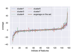
Figure 6: (to be viewed in color) Average of the Jacobian difference vector of highly correlated cluster set. The thicker smooth curve depicts the average on the whole set. The other curves show the average on each cluster of that particular set. Left: First cluster subset. Right: Second cluster subset

As described in the section illustrating the consensus-based interpretabilty method, we group highly correlated clusters to achieve more robust interpretations. On this dataset, we have considered two subsets of highly correlated clusters among 8 representative clusters by our clustering algorithm. Fig. 6 depicts the averages of these subsets along with individual cluster averages. The higher values (i.e., extreme values - leftmost negative or rightmost positive ones) of the average vector correspond to the most relevant and important features. Since they are highly correlated, we notice similar behavior to the average on the subset for each of the clusters. Based on the sorted average of the first subset, we observe that leftmost features in the list have negative impact and rightmost features have positive impact on the positive class (“died within a year”). For the second subset, we notice almost identical features with the positive and negative impact on the positive class. To interpret validation samples, we look at the correlations with each subset.

As a result, we have found that a specific set of features contributes positively to the “died within a year” class while some other set of features contributes positively to the “did not die within a year” class. Also, some features show neutral behavior to the classification task, which are placed in the middle of the spectrum with slight tendencies towards either positive or negative ends of the spectrum. Due to space limitations, we illustrate the contributions of only selected features. We have excluded ethnicity and religion-related features since most of them show neutral effect on the prediction outcome. Table 3 shows some examples of the most positive, negative features contributing to the positive class.

Note that the proposed algorithm is inherently scalable. Computing Jacobian is done implicitly by backpropagation; as such, the Jacobian difference vectors can be computed similarly to training the models for one epoch using mini batches. Furthermore, datasets of billion vectors can be clustered efficiently using product and residual vector quantization techniques (e.g., Matsui et al. [2017]).

n-features
(top n/2 pos, top n/2 neg)	10	20	30	40	50	60	70	80	90	100
SVM	0.8	0.7	0.8	0.725	0.68	0.683	0.728	0.762	0.777	0.8
LR	0.9	0.7	0.766	0.675	0.62	0.683	0.7	0.762	0.766	0.78

Table 5: Comparison of the similarity of resulting feature-importance list from intrinsically interpretable models and proposed consensus-based deep model.

Interpretability Evaluation

Any method for enhancing the interpretability of black-box models has to be rigorously evaluated. Measuring interpretability is not a straightforward process as there is no agreed-upon definition of interpretability in machine learning yet [Doshi-Velez and Kim, 2017]. We base our evaluation of interpretability on the work of  Yang, Du, and Hu [2019], considering three criteria: generalizability, fidelity, and persuasibility. Also, we compare the interpretability of our model with two conventional machine learning models, i.e., support vector machine (SVM) and logistic regression (LR), as the baseline methods.

Evaluation On Generalizability

The proposed interpretability method in this paper is based on the intrinsic characteristics of the activation functions used in each individual deep model (either ReLU or tanh). These activation functions either show locally linear or approximately linear behavior. Thus we consider this model to be semi-intrinsically interpretable.  Yang, Du, and Hu [2019] define the generalizability evaluation of intrinsic interpretability task to be equivalent to the model evaluation using performance evaluation metrics such as accuracy, precision, and recall. According to the aforementioned results, the proposed consensus-based model significantly outperforms shallow models as well as the 5 individual deep-learning-based models.

Evaluation On Fidelity

In a previous section, we demonstrate how the proposed consensus-based algorithm can effectively reject irrelevant samples. To further examine this capability of the proposed algorithm, similar experiments are conducted on the MNIST image dataset. The proposed algorithm can successfully reject adversarial and irrelevant samples. Further details can be found in the previous version of the work.

Evaluation On Persuasibility

A cardiologist, which is a co-author of this paper evaluates the validity of the interpretability method in the real-world setting. These evaluations show that if a patient has issues with other organ systems, he/she is in higher risk for developing a positive outcome (”die within a year”) with the exception of infection and endocrinology. In general, this indicates that a patient with issues with other organs is more susceptible to complications (i.e., comorbidities) along with AMI. Anemia diagnosed by hematocrit seems to significantly increase the risk of one-year mortality (positive outcome). Anemia defined by hemoglobin seems to be weakly predictive of one-year mortality. Liver and kidney dysfunction seem to be indicative of significant increased risk of one-year mortality which is consistent with the fact that the patient is generally sicker and has more critical conditions. Also, a cluster of procedures performed on patients decreases the risk of one-year mortality. This suggests that invasive procedures can decrease such a risk. In addition, two observations are noted. The first observation is about the procedures’ naming in the data set. The lack of sufficient granularity of medical controlled vocabularies for coding procedure makes it difficult to interpret the importance of these procedures in the interpretability results. Also, some of the features that are strongly indicative of higher risk of one-year mortality seem to have an average within the normal range across the population. However, a closer look at their distribution profile in each class suggests that a slight deviation from the normal range associated with these features can enhance the risk for one-year mortality.

Comparisons with Baseline Evaluations

Linear SVM and LR are considered to have intrinsic interpretability  [Friedler et al., 2019] and are quite popular for health data analysis [Wang et al., 2018]. We also try the clusters of SVM (CSVM) by Gu and Han [2013] to check if this ensemble method improves the performance of the shallow learner for this particular classification task. We set the number of clusters to 10 and observe that increasing it does not significantly enhance the model performance. Table 4 includes a comparison of the performance of LR, SVM, CSVM, and the proposed consensus-based algorithm. To compare the feature-importance list as a result of interpretability enhancement of the consensus-based model to that of baseline models, we group features into top-n-features from n=10 to n=100 with step-size=10 and then calculate the percentage of similarity ($\sharp$ features ranked with same priority by both models/n). The detailed comparison is provided in Table 5. On average, the proposed consensus-based model shows 0.73 agreement with LR and 0.74 agreement with SVM on the feature-importance. These results confirm the fact that the proposed model shows linear behavior in local regions.

Related Work

The lack of interpretability of deep neural networks is a limiting factor of their adoption by healthcare and clinical practices. Improving interpretability while retaining high accuracy of deep neural networks is inherently challenging. Existing interpretability enhancement methods can be categorized into integrated and post-hoc approaches [Adadi and Berrada, 2018]. The integrated methods utilize intrinsically interpretable models [Melis and Jaakkola, 2018] but they usually suffer from lower performance compared to deep models. In contrast, the post-hoc interpretation methods attempt to provide explanations on an uninterpretable black-box model [Koh and Liang, 2017]. Such techniques can be further categorized into local and global interpretation ones. The local interpretation methods determine the importance of specific features to the overall performance of the model. The interpretable models are those that can explain why the system results in a specific prediction. This is different from the global interpretability approach, which provides a certain level of transparency about the whole model [Du, Liu, and Hu, 2018]. The proposed method has the advantages of both local and global ones. Our method relies on the local Jacobian difference vector to capture the importance of input features. At the same time, clusters of the difference vectors capture robust model behavior supported by multiple training samples, reducing the complexity while retaining high accuracy.

Conclusion and Future Work

In this paper, we have proposed an interpretability method by clustering local linear models of multiple models, capturing feature importance compactly using cluster means. Using consensus of multiple models allows us to improve classification accuracy and interpretation robustness. Furthermore, the proposed deep ($n$, $k$) consensus algorithm overcomes overgeneralization to irrelevant inputs and oversensitivity to adversarial examples, which is necessary to be able to have meaningful interpretations. For critical applications such as health care, it would be essential if causal relationships between features and the outcomes can be identified and verified using existing medical knowledge. This is being further investigated.

References

- Adadi and Berrada [2018] Adadi, A., and Berrada, M. 2018. Peeking inside the black-box: A survey on explainable artificial intelligence (xai). IEEE Access 6:52138–52160.
- Ahmad, Eckert, and Teredesai [2018] Ahmad, M. A.; Eckert, C.; and Teredesai, A. 2018. Interpretable machine learning in healthcare. In Proceedings of the 2018 ACM International Conference on Bioinformatics, Computational Biology, and Health Informatics, 559–560. ACM.
- Allen-Zhu, Li, and Liang [2018] Allen-Zhu, Z.; Li, Y.; and Liang, Y. 2018. Learning and generalization in overparameterized neural networks, going beyond two layers. CoRR abs/1811.04918.
- Barrett et al. [2019] Barrett, L. A.; Payrovnaziri, S. N.; Bian, J.; and He, Z. 2019. Building computational models to predict one-year mortality in icu patients with acute myocardial infarction and post myocardial infarction syndrome. AMIA Summits on Translational Science Proceedings 2019:407.
- Benjamin et al. [2018] Benjamin, E. J.; Virani, S. S.; Callaway; et al. 2018. Heart disease and stroke statistics-2018 update: a report from the american heart association. Circulation 137(12):e67.
- DeSalvo et al. [2006] DeSalvo, K. B.; Bloser, N.; Reynolds, K.; He, J.; and Muntner, P. 2006. Mortality prediction with a single general self-rated health question: A meta-analysis. Journal of general internal medicine 21(3):267–275.
- Doshi-Velez and Kim [2017] Doshi-Velez, F., and Kim, B. 2017. Towards a rigorous science of interpretable machine learning. arXiv preprint arXiv:1702.08608.
- Du, Liu, and Hu [2018] Du, M.; Liu, N.; and Hu, X. 2018. Techniques for interpretable machine learning. arXiv preprint arXiv:1808.00033.
- Friedler et al. [2019] Friedler, S. A.; Roy, C. D.; Scheidegger, C.; and Slack, D. 2019. Assessing the local interpretability of machine learning models. arXiv preprint arXiv:1902.03501.
- Goodfellow, Shlens, and Szegedy [2014] Goodfellow, I. J.; Shlens, J.; and Szegedy, C. 2014. Explaining and harnessing adversarial examples. arXiv preprint arXiv:1412.6572.
- Gu and Han [2013] Gu, Q., and Han, J. 2013. Clustered support vector machines. In Artificial Intelligence and Statistics, 307–315.
- Johnson et al. [2016] Johnson, A. E.; Pollard, T. J.; Shen, L.; Li-wei, H. L.; Feng, M.; Ghassemi, M.; Moody, B.; Szolovits, P.; Celi, L. A.; and Mark, R. G. 2016. Mimic-iii, a freely accessible critical care database. Scientific data 3:160035.
- Ju, Bibaut, and van der Laan [2017] Ju, C.; Bibaut, A.; and van der Laan, M. J. 2017. The Relative Performance of Ensemble Methods with Deep Convolutional Neural Networks for Image Classification. arXiv e-prints arXiv:1704.01664.
- Kawaguchi et al. [2018] Kawaguchi, K.; Benigo, Y.; Verma, V.; and Pack Kaelbling, L. 2018. Towards understanding generalization via analytical learning theory.
- Koh and Liang [2017] Koh, P. W., and Liang, P. 2017. Understanding black-box predictions via influence functions. In Proceedings of the 34th International Conference on Machine Learning-Volume 70, 1885–1894. JMLR. org.
- LeCun, Bengio, and Hinton [2015] LeCun, Y.; Bengio, Y.; and Hinton, G. 2015. Deep learning. Nature 521(7553):436–444.
- Lecun et al. [1998] Lecun, Y.; Bottou, L.; Bengio, Y.; and Haffner, P. 1998. Gradient-based learning applied to document recognition. Proceedings of the IEEE 86(11):2278–2324.
- L’heureux et al. [2017] L’heureux, A.; Grolinger, K.; Elyamany, H. F.; and Capretz, M. A. 2017. Machine learning with big data: Challenges and approaches. IEEE Access 5:7776–7797.
- Makary and Daniel [2016] Makary, M. A., and Daniel, M. 2016. Medical error—the third leading cause of death in the us. Bmj 353:i2139.
- Matsui et al. [2017] Matsui, Y.; Ogaki, K.; Yamasaki, T.; and Aizawa, K. 2017. Pqk-means: Billion-scale clustering for product-quantized codes. CoRR.
- McNamara et al. [2016] McNamara, R. L.; Kennedy, K. F.; Cohen, D. J.; Diercks, D. B.; Moscucci, M.; Ramee, S.; Wang, T. Y.; Connolly, T.; and Spertus, J. A. 2016. Predicting in-hospital mortality in patients with acute myocardial infarction. Journal of the American College of Cardiology 68(6):626–635.
- Melis and Jaakkola [2018] Melis, D. A., and Jaakkola, T. 2018. Towards robust interpretability with self-explaining neural networks. In Advances in Neural Information Processing Systems, 7786–7795.
- Members et al. [2012] Members, A. F.; Steg, P. G.; James; et al. 2012. ESC Guidelines for the management of acute myocardial infarction in patients presenting with ST-segment elevation: The Task Force on the management of ST-segment elevation acute myocardial infarction of the European Society of Cardiology (ESC). European Heart Journal 33(20):2569–2619.
- Neyshabur et al. [2018] Neyshabur, B.; Li, Z.; Bhojanapalli, S.; LeCun, Y.; and Srebro, N. 2018. Towards understanding the role of over-parametrization in generalization of neural networks. CoRR.
- Reed, Rossi, and Cannon [2017] Reed, G. W.; Rossi, J. E.; and Cannon, C. P. 2017. Acute myocardial infarction. The Lancet 389(10065):197–210.
- Shickel et al. [2017] Shickel, B.; Tighe, P. J.; Bihorac, A.; and Rashidi, P. 2017. Deep ehr: a survey of recent advances in deep learning techniques for electronic health record (ehr) analysis. IEEE journal of biomedical and health informatics 22(5):1589–1604.
- Simonyan, Vedaldi, and Zisserman [2013] Simonyan, K.; Vedaldi, A.; and Zisserman, A. 2013. Deep inside convolutional networks: Visualising image classification models and saliency maps. arXiv preprint arXiv:1312.6034.
- Steele et al. [2018] Steele, A. J.; Denaxas, S. C.; Shah, A. D.; Hemingway, H.; and Luscombe, N. M. 2018. Machine learning models in electronic health records can outperform conventional survival models for predicting patient mortality in coronary artery disease. PloS one 13(8):e0202344.
- Sundararajan, Taly, and Yan [2017] Sundararajan, M.; Taly, A.; and Yan, Q. 2017. Axiomatic attribution for deep networks. In Proceedings of the 34th International Conference on Machine Learning, 3319–3328. PMLR.
- Wang et al. [2018] Wang, J.; Li, L.; Yang, P.; Chen, Y.; Zhu, Y.; Tong, M.; Hao, Z.; and Li, X. 2018. Identification of cervical cancer using laser-induced breakdown spectroscopy coupled with principal component analysis and support vector machine. Lasers in medical science 33(6):1381–1386.
- Wu, Zhu, and Weinan [2017] Wu, L.; Zhu, Z.; and Weinan, E. 2017. Towards understanding generalization of deep learning: Perspective of loss landscapes. CoRR abs/1706.10239.
- Xie et al. [2013] Xie, S.; Kong, X.; Gao, J.; Fan, W.; and Yu, P. S. 2013. Multilabel consensus classification. In 2013 IEEE 13th International Conference on Data Mining, 1241–1246.
- Yang, Du, and Hu [2019] Yang, F.; Du, M.; and Hu, X. 2019. Evaluating explanation without ground truth in interpretable machine learning. arXiv preprint arXiv:1907.06831.
- Zhang et al. [2016] Zhang, C.; Bengio, S.; Hardt, M.; Recht, B.; and Vinyals, O. 2016. Understanding deep learning requires rethinking generalization. CoRR abs/1611.03530.
- Zhang, Nian Wu, and Zhu [2018] Zhang, Q.; Nian Wu, Y.; and Zhu, S.-C. 2018. Interpretable convolutional neural networks. In Proceedings of the IEEE Conference on Computer Vision and Pattern Recognition, 8827–8836.