Improving the NRTidal model for binary neutron star systems

Abstract

Accurate and fast gravitational waveform (GW) models are essential to extract information about the properties of compact binary systems that generate GWs. Building on previous work, we present an extension of the NRTidal model for binary neutron star (BNS) waveforms.
The upgrades are: (i) a new closed-form expression for the tidal contribution to the GW phase which includes further analytical knowledge and is calibrated to more accurate numerical relativity data than previously available; (ii) a tidal correction to the GW amplitude; (iii) an extension of the spin-sector incorporating equation-of-state-dependent finite size effects at quadrupolar and octupolar order; these appear in the spin-spin tail terms and cubic-in-spin terms, both at 3.5PN.
We add the new description to the precessing binary black hole waveform model IMRPhenomPv2 to obtain a frequency-domain precessing binary neutron star model. In addition, we extend the SEOBNRv4_ROM and IMRPhenomD aligned-spin binary black hole waveform models with the improved tidal phase corrections. Focusing on the new IMRPhenomPv2_NRTidalv2 approximant, we test the model by comparing with numerical relativity waveforms as well as hybrid waveforms combining tidal effective-one-body and numerical relativity data. We also check consistency against a tidal effective-one-body model across large regions of the BNS parameter space.

I Introduction

The first gravitational wave (GW) signal associated with electromagnetic (EM) counterparts, detected on the 17th of August 2017, marks a breakthrough in the field of multi-messenger astronomy Abbott et al. (2017, 2017, 2017). Analyses of the GW and EM signatures favor a binary neutron star (BNS) coalescence, e.g., Tanaka et al. (2017); Nicholl et al. (2017); Tanvir et al. (2017); Perego et al. (2017); Waxman et al. (2018); Metzger et al. (2018); Abbott et al. (2019); Kawaguchi et al. (2018); Hinderer et al. (2018); Coughlin et al. (2018); Coughlin and Dietrich (2019); Siegel (2019). Due to the increasing sensitivity of advanced GW detectors, multiple detections of merging BNSs are expected in the near future Abbott et al. (2018).

A prerequisite to extract information from the data are theoretical predictions about the emitted GW signal. The properties of the system are typically inferred via a coherent Bayesian analysis based on cross-correlation of the measured strain with predicted waveform approximants, e.g., Veitch et al. (2015). These cross-correlations are done for a large number of target waveforms and require large computational resources. Thus, the computation of each individual waveform needs to be efficient and fast to ensure that the Bayesian parameter estimation of signals, containing several thousand GW cycles (as typical for BNS systems), is at all manageable. On the other hand, waveform models need to be accurate enough to allow a correct estimate of the source properties, such as the masses, the spins, and internal structure of the NSs.

Over the last years, there has been significant progress modeling the GW signal associated with the BNS coalescence, including the computation of higher-order tidal corrections or spin-tidal coupling, e.g., Refs. Damour et al. (2012); Pani et al. (2018); Banihashemi and Vines (2018); Abdelsalhin et al. (2018); Landry (2018); Jiménez Forteza et al. (2018), and improved accuracy of BNS numerical relativity (NR) simulations Hotokezaka et al. (2015); Bernuzzi and Dietrich (2016); Kiuchi et al. (2017); Dietrich et al. (2018, 2018); Foucart et al. (2019). However, although the analytical progress has improved the performance of post-Newtonian (PN) waveform approximants, PN models still become increasingly inaccurate towards the merger, e.g. Bernuzzi et al. (2012); Favata (2014); Wade et al. (2014); Hotokezaka et al. (2016); Dietrich et al. (2019); Dudi et al. (2018); Samajdar and Dietrich (2018).

Most of the current time-domain tidal waveform models Bernuzzi et al. (2015); Hotokezaka et al. (2015); Hinderer et al. (2016); Steinhoff et al. (2016); Nagar et al. (2018); Nagar and Rettegno (2019); Akcay et al. (2019); Nagar et al. (2019) are based on the effective-one-body (EOB) description of the general relativistic two-body problem Buonanno and Damour (1999); Damour and Nagar (2010). This approach has proven to be able to predict the BNS merger dynamics in large regions of the BNS parameter space, but recent numerical relativity (NR) data revealed configurations for which further improvements of the tidal EOB models are required Hotokezaka et al. (2015); Dietrich and Hinderer (2017); Akcay et al. (2019). While one can expect that over the next years, these issues will be overcome due to further progress in the fields of NR, gravitational self-force, and PN theory, the high computational cost for a single EOB waveform is yet another disadvantage. One possibility to speed up the EOB computation is the use of high-order post-adiabatic approximations of the EOB description to allow an accurate and efficient evaluation of the waveform up to a few orbits before merger Nagar and Rettegno (2019). The other possibility, and most common approach, is constructing reduced-order-models Lackey et al. (2017, 2019). Those models allow the fast computation of waveforms in the frequency domain and are well suited for a direct use in parameter estimation pipelines.

In addition to PN and EOB approximants, there have been proposals for alternative ways to describe tidal GW signals. Refs. Lackey et al. (2014); Pannarale et al. (2013) develop phenomenological black hole-neutron star (BHNS) approximants based on NR data. Ref. Barkett et al. (2016) transforms NR simulations of binary black hole (BBH) systems by adding PN tidal effects, and Refs. Lange et al. (2017, 2018) develop a method to employ NR waveforms or computationally expensive waveform approximants (such as tidal EOB waveforms) directly for parameter estimation.

Another approach to describe BNS systems was presented in Ref. Dietrich et al. (2017), in which BBH models have been augmented by an analytical closed-form expression correcting the GW phase to include tidal effects. This waveform model Dietrich et al. (2017, 2019), referred to as NRTidal, was implemented in the LSC Algorithm Library (LAL) LIGO Scientific Collaboration and Virgo Collaboration (2018) to support the analysis of GW170817 by the LIGO and Virgo Collaborations (LVC) Abbott et al. (2017, 2019, 2018, 2018, 2019) and has also been used outside the LVC, e.g. Dai et al. (2018); Radice and Dai (2019). In addition, Ref. Kawaguchi et al. (2018) developed an alternative tidal approximant in the frequency domain combining EOB and NR information following a similar idea as in Ref. Dietrich et al. (2017).

Studies showed that for GW170817, with its signal-to-noise ratio (SNR) of $\sim 30$, waveform model systematics are within the statistical uncertainties, i.e., that different employed tidal GW models give slightly different, but consistent constraints on the binary properties, e.g., Abbott et al. (2019). However, systematic effects will grow for an increasing number of detections or GW observations with larger SNRs Dudi et al. (2018); Samajdar and Dietrich (2018). Ref. Samajdar and Dietrich (2018) stated that for a GW170817-like event measured with the anticipated design sensitivity of the Advanced LIGO and Advanced Virgo detectors, systematic effects will dominate and the extracted equation of state (EOS) constraints between existing waveform approximants will become inconsistent. Furthermore, the analysis presented in Ref. Dietrich et al. (2019); Dudi et al. (2018) showed that the original NRTidal model could potentially underestimate tidal deformabilities, leading to possible biases for future detections with larger SNRs.

Therefore, to further push for the availability of a fast and accurate waveform model employable for the upcoming observing runs in the advanced detector era, after recalling the basics of NRTidal and discussing the NR simulations and hybrid waveform construction in Sec. II, we improve the NRTidal description by:

1. Recalibrating the closed-form phenomenological tidal description including additional analytical knowledge and using improved NR data (Sec. III.1);

2. Adding a tidal GW amplitude correction to the model (Sec. III.2);

3. Incorporating EOS-dependent 3.5PN spin-spin and cubic-in-spin effects proportional to the quadrupole and octupole moments of the NSs Marsat (2015); Bohé et al. (2015); Krishnendu et al. (2017); Nagar et al. (2019) (Sec. III.3).

We validate the new NRTidalv2 approximant with a set of $10$ high-resolution NR waveforms (Sec. IV.1) and $18$ hybrids of NR waveforms and the TEOBResumS tidal EOB model Nagar et al. (2018) (Sec. IV.2). Furthermore, we compare the model in a larger region of the parameter space than currently covered with NR simulations by computing the mismatch with respect to the SEOBNRv4T tidal EOB model Hinderer et al. (2016); Steinhoff et al. (2016) (Sec. IV.3). We note that for this waveform model Ref. Lackey et al. (2019) recently developed a reduced order model which can also be used directly for GW data analysis. We conclude in Sec. V. In the Appendices, we discuss possible extensions to the model, considering the tidal amplitude correction (Appendix A) and the mass ratio dependence of the tidal phase (Appendix B).

In this article geometric units are used by setting $G=c=M_{\odot}=1$. At some places units are given explicitly to allow a better interpretation. Further notations are $M=M_{A}+M_{B}$ for the total mass of the system, $\chi_{A},\chi_{B},\Lambda_{A},\Lambda_{B}$ for the individual dimensionless spins and tidal deformabilities of the stars. The mass ratio of the system is $q=M_{A}/M_{B}$ and the symmetric mass ratio is $\nu=M_{A}M_{B}/(M_{A}+M_{B})^{2}$. We define the labeling of the individual stars so their masses satisfy $M_{A}\geq M_{B}$.

II Basic ideas and improved numerical relativity data

II.1 The basic idea of NRTidal

During the BNS coalescence, each star gets deformed due to the gravitational field of the companion. These tidal deformations accelerate the inspiral and leave a clear imprint in the GW signal, e.g., Flanagan and Hinderer (2008). Consequently, the theoretical modeling of BNSs and the extraction of tidal effects from measured GW signals is an important way of determining the internal structure of NSs and thus the EOS of supranuclear dense matter.

The complex time-domain GW signal is given by

$$h(t)=A(t)e^{-{\rm i}\phi(t)},$$ (1)

with amplitude $A(t)$ and time-domain phase $\phi(t)$. Here we only consider the dominant $2,2$ [spin $(-2)$ weighted spherical harmonic] mode. We assume in the following that the phase can be decomposed into

$$\phi(\hat{\omega})=\phi_{\rm pp}(\hat{\omega})+\phi_{\rm SO}(\hat{\omega})+\phi_{\rm SS}(\hat{\omega})+\phi_{\rm T}(\hat{\omega})+\cdots\ ,$$ (2)

where the dimensionless GW frequency is given by $\hat{\omega}=M\omega=M\partial_{t}\phi(t)$. Here $\phi_{\rm pp}$ denotes the nonspinning, point-particle, contribution to the overall phase, $\phi_{\rm SO}$ corresponds to contributions caused by spin-orbit coupling, $\phi_{\rm SS}$ corresponds to contributions caused by spin-spin effects (both self-spin and spin-interactions), and $\phi_{\rm T}$ denotes the tidal effects present in the GW phase.

Similar to Eq. (1), the waveform can be written in the frequency domain as

$$\tilde{h}(f)=\tilde{A}(f)e^{-{\rm i}\psi(f)},,$$ (3)

with GW frequency $f$ and frequency domain amplitude $\tilde{A}(f)$ and phase $\psi(f)$. Here we assume again:

$$\psi(\hat{\omega})=\psi_{\rm pp}(\hat{\omega})+\psi_{\rm SO}(\hat{\omega})+\psi_{\rm SS}(\hat{\omega})+\psi_{\rm T}(\hat{\omega})+\cdots\ .$$ (4)

Constraints on the supranuclear EOS governing the matter inside NSs rely on an accurate measurement of the tidal phase contribution. This contribution enters first at the 5th PN order.

The main idea of the NRTidal approach is to provide a closed-form approximation for the tidal phase $\phi_{\rm T}$ or $\psi_{\rm T}$. Because standard GW data analysis is carried out in the frequency domain, the frequency domain model is of particular importance, due to its efficiency. In addition to the tidal contribution, the final NRTidal approximant also incorporates EOS dependent effects in $\psi_{\rm SS}$, since the spin-spin contributions depend on the quadrupole and higher moments of the individual stars, and thus on the internal structure of the stars.

We note that there are higher-order spin-tidal coupling effects that have recently been computed Abdelsalhin et al. (2018); Landry (2018). However, as outlined in Jiménez Forteza et al. (2018), these terms will be unmeasurable in the advanced GW detector era. Therefore, we do not include them in the current description to avoid unnecessary computational costs.

II.2 High-precision NR simulations

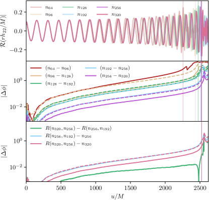
Figure 1: New high-resolution NR data employed for the calibration of the NRTidalv2 approximant. Top panel: Real part of the GW signal for the six different resolutions employing $64$, $96$, $128$, $192$, $256$, and $320$ points in the refinement levels covering the individual NSs. The waveforms shown are already extrapolated to spatial infinity to correct for the finite radius extraction; see Bernuzzi and Dietrich (2016) for more details (we use $K=1$ here). Middle panel: Phase difference between different resolutions. Bottom panel: Phase difference between different Richardson extrapolated waveforms or between a Richardson extrapolated waveforms and the waveform from an individual resolution. The vertical lines in each panel refer to the time of merger, i.e., the peak time of the GW amplitude for the individual resolutions. The dashed lines in the bottom two panels show the phase difference scaled to the next lowest pair of resolutions assuming second order convergence. $u$ denotes the retarded time.

The field of NR has made significant progress over the last years. Nevertheless, the production of highly accurate gravitational BNS waveforms remains challenging and there exist only a small number of simulations with low eccentricity and with phase errors small enough to allow GW modeling; cf. Refs. Hotokezaka et al. (2015); Bernuzzi and Dietrich (2016); Dietrich et al. (2018, 2018); Kiuchi et al. (2017); Foucart et al. (2019).

In addition to the dataset used for the original NRTidal calibration Dietrich et al. (2017, 2019), we performed one additional simulation for a non-spinning equal-mass BNS setup employing a piecewise-polytropic parametrization of the SLy Read et al. (2009) EOS. This EOS is in agreement with recent constraints extracted from GW170817 Abbott et al. (2018, 2018); Bauswein et al. (2017); Most et al. (2018); Radice and Dai (2019); Coughlin et al. (2018) and thus is a natural choice for our work. The same physical configuration has already been used in the past for the construction of the NRTidal model Dietrich et al. (2017, 2018); cf. Table 1 for further details. In Dietrich et al. (2017, 2018), we have simulated this setup with the BAM code Brügmann et al. (2008); Thierfelder et al. (2011); Dietrich et al. (2015); Bernuzzi and Dietrich (2016) for $5$ different resolutions with $64$, $96$, $128$, $192$, and $256$ points in the finest refinement level covering the individual NSs. Here, we add one additional simulation with $320$ points in the finest refinement level. This corresponds to a spatial resolution of $0.047M_{\odot}\approx 70\ \rm m$ and computational costs of $\sim 5$ million CPU-hours for this single resolution.

The availability of six different resolutions and the presence of clean convergence across multiple resolutions allows us to employ Richardson extrapolation to obtain an improved GW signal and to provide an associated error budget; see Ref. Bernuzzi and Dietrich (2016) for more details. We present the GW signal for the different resolutions in Fig. 1 (top panel) and the phase difference and convergence properties in the middle and bottom panels.

Except for the lowest resolution, clean second order convergence is obtained throughout the inspiral. This becomes evident by comparison of the individual phase differences with the phase differences rescaled assuming second order convergence (dashed lines). For the lowest resolution setup ($n_{64}$), second order convergence is lost a few orbits before merger ($u\approx 1500M$). Merger times for each resolution are indicated by vertical solid lines in Fig. 1.

The phase difference between the highest ($n_{320}$) and second highest resolution ($n_{256}$) is $0.52\ \rm rad$ at the moment of merger. Performing a Richardson extrapolation Bernuzzi and Dietrich (2016), we obtain more accurate phase descriptions. We denote the Richardson extrapolated data obtained from the resolutions $n_{X}$ and $n_{Y}$ as $R(n_{X},n_{Y})$. We crosscheck the robustness of the procedure by presenting the phase differences $R(n_{320},n_{256})-n_{320}$ and $R(n_{256},n_{192})-n_{256}$ in the bottom panel of Fig. 1. Rescaling the phase difference of $R(n_{320},n_{256})-n_{320}$ assuming second order convergence shows excellent agreement with $R(n_{256},n_{192})-n_{256}$. This demonstrates that the leading error term scales quadratically with respect to the grid spacing/resolution.

Thus, we can estimate the uncertainty of the Richardson extrapolated waveform $R(n_{320},n_{256})$ to be the difference with the $n_{320}$ resolution. At the moment of merger, this gives an uncertainty of $0.37\ \rm rad$. At this time the estimated error due to the finite radius extraction is below $0.044\ \rm rad$, which leads to a conservatively estimated total error of $\Delta\phi_{\rm mrg}\lesssim 0.38\ \rm rad$ at merger.

An alternative, but not conservative, error measure is given by the difference between the two Richardson extrapolated waveforms (green line in the bottom panel). We find that throughout the inspiral the difference between the $R(n_{320},n_{256})$ and $R(n_{256},n_{192})$ is below $0.1\ \rm rad$ (at the moment of merger $\Delta\phi=0.087\ \rm rad$, which would lead to a total error of $\lesssim 0.1\ \rm rad$ once finite radius extraction is included).

In addition to this new setup, we also consider the additional two high resolution simulations available in the CoRe database Dietrich et al. (2018), cf. Table 1. These setups, CoRe:BAM:0037 and CoRe:BAM:0064, only employ 192 points across the star and have conservatively estimated phase uncertainties at merger of $1.20\ \rm rad$ and $2.27\ \rm rad$, respectively. We incorporated this accuracy difference by weighting the individual setups differently during the construction of the NRTidalv2 phase, as discussed in the next subsection.

II.3 Hybrid Construction

Table 1: The non-spinning BNS and BBH hybrids employed in the construction of the NRTidalv2 model. The columns refer to the name, the employed EOS, the individual masses of the stars $M^{A}$, $M^{B}$, the tidal deformabilities $\Lambda^{A},\Lambda^{B}$, the tidal coupling constant $\kappa^{T}_{\rm eff}$ [Eq. (8)], and the ID in the CoRe and SXS databases.

Name	EOS	$M_{A}$	$M_{B}$	$\Lambda_{A}$	$\Lambda_{B}$	$\kappa^{T}_{\rm eff}$	ID
SLy	SLy	1.350	1.350	392.1	392.1	73.5	CoRe:BAM:0095
H4	H4	1.372	1.372	1013.4	1013.4	190.0	CoRe:BAM:0037
MS1b	MS1b	1.350	1.350	1389.4	1389.4	288.1	CoRe:BAM:0064
BBH	–	1.350	1.350	0	0	0	SXS:BBH:0066

In the original NRTidal work, PN, EOB, and NR approximants have been separately used in different frequency intervals. Here, we start by constructing hybrid waveforms consisting of a time domain tidal EOB model (TEOBResumS) inspiral Nagar et al. (2018) connected to the high resolution NR simulation discussed above. The hybridization is performed as discussed in Refs. Dietrich et al. (2019); Dudi et al. (2018) to which we refer for further details. In addition to the BNS hybrid waveforms, we also create a hybrid between the non-tidal version of the TEOBResumS model and a binary black hole waveform computed with the SpEC code SpE , setup SXS:BBH:0066 of the public SXS catalog Mroué et al. (2013); Blackman et al. (2015). All the hybrids have an initial frequency of $20\ \rm Hz$.

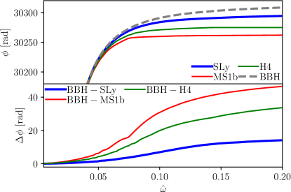
Figure 2: Time domain phase of the hybrid waveforms employed to develop NRTidalv2. The bottom panel shows the phase difference caused by tidal effects.

We present the time domain phase evolution of the BBH and BNS hybrids in Fig. 2. For this plot we align the waveforms at $\sim 22\ \rm Hz$.

We emphasize that only the four hybrid waveforms listed in Table 1 are used for calibration of the NRTidalv2 model, where the dataset we are going to fit is

$$\begin{split}\phi_{T}^{\rm NR}&=\frac{1}{320+192+192}\bigg{[}320(\phi_{\rm SLy}-\phi_{\rm BBH})+192(\phi_{\rm H4}-\phi_{\rm BBH})\\ &\quad+192(\phi_{\rm MS1b}-\phi_{\rm BBH})\bigg{]}\\ &=\frac{1}{11}\bigg{(}5\phi_{\rm SLy}+3\phi_{\rm H4}+3\phi_{\rm MS1b}-11\phi_{\rm BBH}\bigg{)}.\end{split}$$ (5)

The factors are obtained by linearly weighting the resolutions of the individual NR data, i.e., 320 points accross the star for the SLy setup and 192 for H4 and MS1b setups. We decided to use this minimal dataset since these are the available data with the highest accuracy. Note that a simple restriction to the highest resolution, i.e., the SLy data, leads to a phase description which does not accurately characterize binaries with large tidal deformabilities. Thus, it would be preferable to include in the future a larger number of NR simulations with varying masses, spins, mass ratios, and EOSs once these are available. However, while there are a small number of high quality waveforms Dietrich et al. (2018), these waveforms do not span a sufficiently large region of the parameter space to incorporate additional mass ratio, EOS, or mass dependencies in our phenomenological ansatz.

III Improvements

The NRTidalv2 approach can be added to any BBH model: we focus our discussion here on the frequency-domain IMRPhenomPv2, IMRPhenomD, and SEOBNRv4_ROM models. We primarily concentrate on the extension of IMRPhenomPv2 Hannam et al. (2014); Khan et al. (2016) describing precessing systems. In addition, we have also added the improved tidal phase description to the SEOBNRv4_ROM Bohé et al. (2017) and the IMRPhenomD Khan et al. (2016) approximants. For SEOBNRv4_ROM and IMRPhenomD, we decided to include only the tidal phase description to reduce additional computational costs and allow a faster computation of waveforms than for IMRPhenomPv2_NRTidalv2.

We present an overview of all existing NRTidal models in Table 2.

Table 2: Overview of the existing NRTidal approximants. The individual columns refer to: the name of the approximant, the BBH baseline, the employed tidal phase, the employed spin-spin and cubic-in-spin contribution, employed tidal amplitude corrections, and the incorporation of precession, as well as the computational time $\Delta T_{\rm f_{min}}$ of the model to produce a single waveform for a non-spinning, equal mass binary with individual masses $M_{A,B}=1.35$ and $\Lambda_{A,B}=400$ on an Intel Xeon E5-2630v3 processor for various starting frequencies.

LAL approximant name	BBH baseline	$\psi_{T}$	spin-spin	cubic-in-spin	tidal amp.	precession	$\Delta T_{\rm f_{min}}\ \rm[s]$
							$10\rm\ Hz$	$20\rm\ Hz$	$30\rm\ Hz$	$40\rm\ Hz$
IMRPhenomD_NRTidal	IMRPhenomD	NRTidal	up to 3PN (BBH)	✗	✗	✗	2.55	0.29	0.14	0.07
IMRPhenomD_NRTidalv2	IMRPhenomD	NRTidalv2	up to 3PN	✗	✗	✗	2.54	0.29	0.14	0.07
SEOBNRv4_ROM_NRTidal	SEOBNRv4_ROM	NRTidal	up to 3PN	✗	✗	✗	3.39	0.40	0.18	0.09
SEOBNRv4_ROM_NRTidalv2	SEOBNRv4_ROM	NRTidalv2	up to 3PN	✗	✗	✗	3.34	0.40	0.18	0.09
IMRPhenomPv2_NRTidal	IMRPhenomPv2	NRTidal	up to 3PN	✗	✗	✓	7.30	0.90	0.43	0.21
IMRPhenomPv2_NRTidalv2	IMRPhenomPv2	NRTidalv2	up to 3.5PN	up to 3.5PN	✓	✓	8.56	1.06	0.51	0.28

III.1 Recalibrating the NRTidal phase

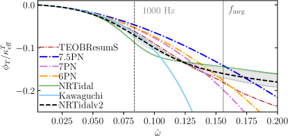
Figure 3: Time domain tidal phase contribution divided by the tidal coupling constant $\kappa^{T}_{\rm eff}$. We show as a gray shaded region the parameter space covered by our hybrids (Table 1) and as a dashed gray line the SLy hybrid’s tidal phase divided by the coupling constant for this setup. In addition, the 6PN (orange), 7PN (orchid), and 7.5PN (blue) tidal phase estimates, as well as the original NRTidal Dietrich et al. (2017) (green) and Kawaguchi et al. Kawaguchi et al. (2018) (cyan) approximants are presented. As a dark red line, we present an estimate obtained using the tidal EOB model TEOBResumS. We note that the Kawaguchi et al. and TEOBResumS tidal phases depend on $\tilde{\Lambda}$ even after being scaled by the coupling constant; for this plot and the following ones we use $\tilde{\Lambda}=392.1$ to describe the SLy configuration. NRTidalv2 is shown with a black dashed line. We mark the frequencies of $1000\ \rm Hz$ and the merger frequency corresponding to our SLy setup, described in Table 1.

III.1.1 Ansatz for the NRTidal time-domain phase

Non-spinning tidal contributions start entering the GW phasing at the 5PN order and partially known analytical knowledge exists up to 7.5PN Damour et al. (2012):

$$\phi_{T} =-\kappa_{A}c^{A}_{\rm Newt}x^{5/2}\left(1+c^{A}_{1}x+c^{A}_{3/2}x^{3/2}+\right.$$

$$\quad+\left.c^{A}_{2}x^{2}+c_{5/2}^{A}x^{5/2}\right)+[A\leftrightarrow B],$$ (6)

with the dimensionless EOB tidal parameter $\kappa_{A}$ (defined below) and $x(\hat{\omega})=(\hat{\omega}/2)^{2/3}$. The individual coefficients $c_{i}^{A}$ are

$$c^{A}_{\rm Newt} = -\frac{(X_{A}+12X_{B})}{8X_{A}X_{B}^{2}},$$ (7a)

$$c^{A}_{1} = -\frac{5\left(260X_{A}^{3}-2286X_{A}^{2}-919X_{A}+3179\right)}{336\left(11X_{A}-12\right)},$$ (7b)

$$c^{A}_{3/2} = -\frac{5}{2}\pi,$$ (7c)

$$c_{2}^{A} = \left[5\left(67702048X_{A}^{5}-223216640X_{A}^{4}+337457524X_{A}^{3}\right.\right.$$ (7d)

$$\left.\left.-141992280X_{A}^{2}+96008669X_{A}-143740242\right)\right]/$$

$$\left[3048192\left(11X_{A}-12\right)\right],$$

$$c_{5/2}^{A} = -\frac{\pi\left(10232X_{A}^{3}-7022X_{A}^{2}+22127X_{A}-27719\right)}{192\left(11X_{A}-12\right)},$$ (7e)

and similarly with $A\leftrightarrow B$. Here $X_{A,B}=M_{A,B}/M$. We note that although analytic knowledge exists up to the 7.5PN order, some unknown terms are present at 7PN. As discussed in Ref. Damour et al. (2012), these terms are expected to be small and are set to zero in our definition of $c_{2}^{A}$, $c_{2}^{B}$.

As in the original NRTidal description Dietrich et al. (2017, 2018) we introduce the effective tidal coupling constant $\kappa_{\rm eff}^{T}$ which describes the dominant tidal and mass ratio effects:

$$\kappa^{T}_{\rm eff}=\frac{2}{13}\left[\left(1+12\frac{X_{B}}{X_{A}}\right)\left(\frac{X_{A}}{C_{A}}\right)^{5}k^{A}_{2}+(A\leftrightarrow B)\right]\ ,$$ (8)

where $C_{A,B}\equiv M_{A,B}/R_{A,B}$ are the compactnesses of the stars at isolation, and $k^{A,B}_{2}$ the Love numbers describing the static quadrupolar deformation of one body in the gravitoelectric field of the companion Damour (1983); Hinderer (2008); Damour and Nagar (2009); Binnington and Poisson (2009). The parameter $\kappa^{T}_{\rm eff}$ is related to $\tilde{\Lambda}$ (the mass-weighted tidal deformability commonly used in GW analysis Wade et al. (2014)) by

$$\tilde{\Lambda}=\frac{16}{3}\kappa^{T}_{\rm eff},$$ (9)

and the individual tidal deformability parameters are given by

$$\Lambda_{A,B}=\frac{2}{3}\frac{k_{2}^{A,B}}{C_{A,B}^{5}}.$$ (10)

The EOB tidal parameter used in Eq. (6) is given by $\kappa_{A}=3X_{B}X_{A}^{4}\Lambda_{A}$.

In the following, we restrict the parameters $c_{1}^{A,B},c_{3/2}^{A,B},c_{2}^{A,B},c_{5/2}^{A,B}$ to their equal-mass values (due to the absence of a large set of high-quality unequal mass NR data), and therefore, discard the superscripts $A$ and $B$. For this case, an effective representation of tidal effects is obtained using

$$\phi_{T}(x)=-\kappa_{\rm eff}^{T}\frac{13}{8\nu}x^{5/2}P_{\rm NRTidalv2}(x)\ ,$$ (11)

with the Padé approximant

$$P_{\rm NRTidalv2}(x)=\frac{1+n_{1}x+n_{3/2}x^{3/2}+n_{2}x^{2}+n_{5/2}x^{5/2}+n_{3}x^{3}}{1+d_{1}x+d_{3/2}x^{3/2}+d_{2}x^{2}}.$$ (12)

To enforce consistency with the analytic PN knowledge [Eqs. (6)-(7e)], some of the individual terms are restricted

$$n_{1} = c_{1}+d_{1},$$ (13a)

$$n_{3/2} = \frac{c_{1}c_{3/2}-c_{5/2}-c_{3/2}d_{1}+n_{5/2}}{c_{1}},$$ (13b)

$$n_{2} = c_{2}+c_{1}d_{1}+d_{2},$$ (13c)

$$d_{3/2} = -\frac{c_{5/2}+c_{3/2}d_{1}-n_{5/2}}{c_{1}},$$ (13d)

with

$$c_{1} =\frac{3115}{624},\qquad c_{3/2} =-\frac{5\pi}{2},$$ (14a)

$$c_{2} =\frac{28024205}{1100736},\qquad c_{5/2} =-\frac{4283\pi}{312}.$$ (14b)

The remaining unknown $4$ parameters are fitted to the data:

$$n_{5/2} =312.48173,\qquad n_{3} =-342.15498,$$ (15a)

$$d_{1} =-20.237200,\qquad d_{2} =-5.361630.$$ (15b)

Figure 3 shows our findings. We show as a gray shaded region the parameter space in $\phi_{T}/\kappa_{\rm eff}^{T}$ covered by our simulations, where the gray dashed line refers explicitly to the SLy configuration. Here we do not include any error estimate in the BBH hybrid used to extract the tidal phase. In addition, we present the 6PN tidal contribution, which the old NRTidal approximant reduces to in the low frequency limit; the 7.5PN contribution, which the new NRTidalv2 reduces to in the low frequency limit; and the 7PN contribution, which is the PN approximant showing the best agreement to the NR data. We also show the tidal phase given in Kawaguchi et al. Kawaguchi et al. (2018), which has been calibrated to NR simulations up to a frequency of $1000\ \rm Hz$ (thin dashed line). The model of Ref. Kawaguchi et al. (2018) loses validity outside its calibration region and overestimates tidal effects at the moment of merger, though this would not affect GW data analysis if a maximum frequency of $1000\ \rm Hz$ is employed, or the signal at frequencies $\gtrsim 1000\ \rm Hz$ is sufficiently suppressed by the detectors’ noise. In addition, we find good agreement between the Kawaguchi et al. fit and the new NRTidalv2 approximation below $1000\ \rm Hz$. We also show the estimated tidal phase extracted by comparing our BBH hybrid with a tidal EOB waveform computed for our SLy configuration using the TEOBResumS Nagar et al. (2018) model. The tidal phase estimate of the TEOBResumS model is slightly less attractive for frequencies around $1000\ \rm Hz$, but more attractive at higher frequencies. Finally, the original NRTidal model is shown as a green line. The tidal contribution is overestimated at about $f\sim 1000\ \rm Hz$, and later underestimated. This oscillatory behavior has been seen before, e.g., Dietrich et al. (2017, 2018, 2019), and could potentially lead to biases in the estimate of tidal effects from GW signals Dudi et al. (2018). For both NRTidal and NRTidalv2 the growth of the tidal phase around merger is much smaller than for any other approximant, which generally reduces possible pathologies in more extreme regions of the parameters, e.g., a cancellation of the point-particle and attractive tidal phase close to merger. As expected the NRTidalv2 model stays within the gray shaded region and, thus, close to the numerical relativity dataset used for the calibration.

III.1.2 Frequency domain phase

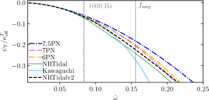
Figure 4: Tidal phase in the frequency domain. We show the 6PN (orange), 7PN (orchid), and 7.5PN (blue) tidal phase estimates, as well as the original NRTidal Dietrich et al. (2017) (green) and the Kawaguchi et al. Kawaguchi et al. (2018) (cyan) approximant. The new model is shown with a black dashed line. We mark the frequencies of $1000\ \rm Hz$ and the merger frequency corresponding to our SLy setup, described in Table 1.

As in Ref. Dietrich et al. (2017) we will employ the stationary phase approximation (SPA), discussed in, e.g., Damour et al. (2012), to derive the tidal phase contribution $\psi_{T}$ in the frequency domain, i.e., we solve

$$\frac{\text{d}^{2}\psi_{T}(\omega)}{\text{d}\omega^{2}}=\frac{1}{\omega}\frac{\text{d}\phi_{T}(\omega)}{\text{d}\omega}$$ (16)

to obtain $\psi_{T}$. Although $\phi_{T}$ is given explicitly, we solve Eq. (16) numerically and approximate the result with a Padé approximant similar to Eqs. (11) and (12):

$$\psi_{T}(x)=-\kappa_{\rm eff}^{T}\frac{39}{16\nu}x^{5/2}\tilde{P}_{\rm NRTidalv2}(x)\ ,$$ (17)

with

$$\tilde{P}_{\rm NRTidalv2}(x)=\frac{1+\tilde{n}_{1}x+\tilde{n}_{3/2}x^{3/2}+\tilde{n}_{2}x^{2}+\tilde{n}_{5/2}x^{5/2}+\tilde{n}_{3}x^{3}}{1+\tilde{d}_{1}x+\tilde{d}_{3/2}x^{3/2}+\tilde{d}_{2}x^{2}},$$ (18)

and

$$\tilde{n}_{1} = \tilde{c}_{1}+\tilde{d}_{1},$$ (19a)

$$\tilde{n}_{3/2} = \frac{\tilde{c}_{1}\tilde{c}_{3/2}-\tilde{c}_{5/2}-\tilde{c}_{3/2}\tilde{d}_{1}+\tilde{n}_{5/2}}{\tilde{c}_{1}},$$ (19b)

$$\tilde{n}_{2} = \tilde{c}_{2}+\tilde{c}_{1}\tilde{d}_{1}+\tilde{d}_{2},$$ (19c)

$$\tilde{d}_{3/2} = -\frac{\tilde{c}_{5/2}+\tilde{c}_{3/2}\tilde{d}_{1}-\tilde{n}_{5/2}}{\tilde{c}_{1}},$$ (19d)

where the known coefficients are:

$$\tilde{c}_{1} =\frac{3115}{1248},\qquad \tilde{c}_{3/2} =-\pi,$$ (20a)

$$\tilde{c}_{2} =\frac{28024205}{3302208},\qquad \tilde{c}_{5/2} =-\frac{4283\pi}{1092}.$$ (20b)

and the fitting coefficients are:

$$\tilde{n}_{5/2} =90.550822,\qquad \tilde{n}_{3} =-60.253578,$$ (21a)

$$\tilde{d}_{1} =-15.111208,\qquad \tilde{d}_{2} =8.0641096.$$ (21b)

We present the final tidal phase contribution in the frequency domain in Fig. 4 for a number of different GW approximants. Fig. 5 shows the corresponding phase differences with respect to the NRTidalv2 model on a double logarithmic scale.

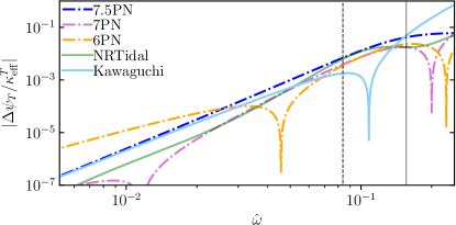
Figure 5: Absolute magnitude of the tidal phase difference between frequency domain approximants and the NRTidalv2 model. The vertical dashed line represents $1000\ \rm Hz$, the frequency up to which the Kawaguchi et al. model was calibrated, and the solid line marks the merger frequency of the SLy setup we consider.

III.2 Tidal amplitude corrections

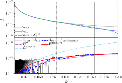
Figure 6: Frequency domain waveform amplitude. Top panel: We show the BBH and BNS hybrids’ amplitudes as well as the BBH amplitude augmented with the 6PN tidal terms presented in Eq. (22). Bottom panel: amplitude differences with the raw data in black and the smoothed data as a blue dashed line. The final NRTidalv2 fit is shown in red. The vertical dashed lines refer to $1000\ \rm Hz$ and to the merger frequency of the BNS hybrid respectively.

The extraction of binary properties relies mostly on the GW phase, which makes an accurate description of $\psi$ the primary target of GW modeling. However, a realistic estimate of the GW amplitude is also of importance, e.g., for a precise distance measurement.

Therefore, we will discuss a possible extension of the NRTidal approach including a tidal amplitude correction in the frequency domain. An alternative time and frequency domain amplitude correction is presented in Appendix A.

Here, we will derive the frequency domain tidal correction from the frequency domain representation of the SLy and BBH TEOBResumS-NR hybrids, described in Table 1. We do not employ the H4 and MS1b setup for the amplitude correction since their lower merger frequencies add additional complications during the construction procedure. The top panel of Fig. 6 shows $\tilde{A}$ for our generic setups and also the BBH result augmented ($\tilde{A}=\tilde{A}_{\rm BBH}+\tilde{A}_{\rm T}$) by the 6PN expression:

$$\tilde{A}_{T}^{\rm 6PN}=\sqrt{\frac{160\pi\nu}{27}}\frac{M^{2}}{D_{L}}\ {\kappa^{T}_{\rm eff}}x^{-7/4}\left(-\frac{27}{16}x^{5}-\frac{449}{64}x^{6}\right),$$ (22)

e.g., Ref. Hotokezaka et al. (2016), where $D_{L}$ is the luminosity distance of the source, which is the appropriate substitution for the effective distance used in Ref. Hotokezaka et al. (2016) for our case. Kawaguchi et al. Kawaguchi et al. (2018) extended Eq. (22) to

$$\begin{split}\tilde{A}_{T}^{\rm Kawaguchi}&=\sqrt{\frac{160\pi\nu}{27}}\frac{M^{2}}{D_{L}}\ {\kappa^{T}_{\rm eff}}x^{-7/4}\\ &\quad\times\left(-\frac{27}{16}x^{5}-\frac{449}{64}x^{6}-4251x^{7.890}\right).\end{split}$$ (23)

Based on the good agreement we have found between the results of Ref. Kawaguchi et al. (2018) and the new NRTidalv2 phase description below $1000\ \rm Hz$, we want to use Eq. (23) as baseline for a possible frequency amplitude extension of the NRTidalv2 approximant.

For this purpose we employ the ansatz

$$\tilde{A}_{T}^{\rm NRTidalv2}=-\sqrt{\frac{5\pi\nu}{24}}\frac{9M^{2}}{D_{L}}\kappa^{T}_{\rm eff}x^{13/4}\frac{1+\frac{449}{108}x+\frac{22672}{9}x^{2.89}}{1+d\ x^{4}}.$$ (24)

Equation (24) ensures that for small frequencies Eq. (23) is recovered, but that the high frequency behavior ($f>1000\ {\rm Hz}$) can be adjusted. We obtain $d=13477.8$ by fitting the data presented in Fig. 6 (blue dashed line in the bottom panel).

As for the previous NRTidal implementation, we add a Planck taper McKechan et al. (2010) to end the inspiral waveform. The taper begins at the estimated merger frequency [Eq. (11) of Dietrich et al. (2019)] and ends at $1.2$ times the merger frequency. Thus, the final amplitude is given as:

$$\tilde{A}=(\tilde{A}_{\rm BBH}+\tilde{A}_{T}^{\rm NRTidalv2})\times\tilde{A}_{\rm Planck}.$$ (25)

Because of the smooth frequency and amplitude evolution even after the moment of merger, this taper only introduces negligible errors and does not lead to biases in the parameter estimation of even SNR 100 signals, as shown using an injection of an SLy hybrid with the same parameters as those considered here in Dudi et al. (2018).

III.3 Incorporating higher-order spin-spin effects

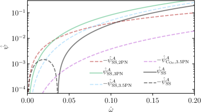
Figure 7: Quadrupolar and octupolar spin-spin and cubic-in spin contributions at 2PN, 3PN, and 3.5PN order, as well as their sum, all without the overall Newtonian scaling. Negative terms are shown with dashed lines, positive terms with solid lines. The plot assumes an equal-mass system with dimensionless spins $\chi_{A}=\chi_{B}=0.2$ and tidal deformabilities of $\Lambda_{A}=\Lambda_{B}=350$. The quadrupole and octupole moments are computed according to Eq. (28) and Eq. (29) ($C_{\rm Q}^{A}=C_{\rm Q}^{B}=4.30$, $C_{\rm Oc}^{A}=C_{\rm Oc}^{B}=7.28$).

While nonspinning NSs and black holes only have a nonzero monopole moment, spinning neutron stars and black holes have an infinite series of nonzero (Geroch-Hansen) multipole moments, e.g., Refs. Pappas and Apostolatos (2014); Yagi et al. (2014). The contributions from the stars’ (mass) monopole and (spin) dipole to the binary’s motion are explicitly accounted for in the BBH baseline. Additionally, contributions from higher spin-induced multipoles in the BBH baseline model are indirectly included due to the calibration to NR simulations. However, without further adjustment, all multipoles would be specialized to the black hole values, which (as shown in Dietrich et al. (2019)) noticeably reduces the accuracy for spinning BNS systems. Thus, to improve the performance of NRTidalv2 for spinning configurations, we include an EOS dependence in the quadrupole and octupole, as these are the moments that appear in current PN calculations. These two moments (in their scalar versions) can be written as $M^{(A,B)}_{2}=-C_{\rm Q}^{A}M_{A,B}^{3}\chi_{A,B}^{2}$, $S_{3}^{(A,B)}=-C_{\rm Oc}^{A,B}M_{A,B}^{4}\chi_{A,B}^{3}$, respectively, for star $A$ and $B$. Here $C_{\rm Q}^{A,B}$ and $C_{\rm Oc}^{A,B}$ are the quadrupolar and octupolar spin-induced deformabilities for the individual stars. Both $C_{\rm Q}$ and $C_{\rm Oc}$ are $1$ for a black hole.

In this paper, we extend the existing LALSuite implementation, which currently contains the EOS dependence of the quadrupole moment only up to 3PN Bohé et al. (2015); Mishra et al. (2016) to include the $3.5$PN spin-squared terms, completed using the recently computed 3.5PN tail terms Nagar et al. (2019). We also include leading order spin-cubed terms entering at 3.5PN order.

The contributions of the quadrupole and octupole deformations of the stars to the binary’s binding energy and energy flux have been computed through $3.5$PN, Refs. Bohé et al. (2015); Marsat (2015); Nagar et al. (2018), building on earlier work reviewed in Blanchet (2014). We compute the phase in the frequency domain using the SPA. These contributions to the phase were already presented in Krishnendu et al. (2017), except the $3.5$PN spin-spin terms, as Krishnendu et al. (2017) did not have the $3.5$PN spin-squared tail term from Ref. Nagar et al. (2018). Explicitly, the self-spin (i.e., $C_{\rm Q}$ and $C_{\rm Oc}$) terms in the phasing that we add to the BBH baseline are

$$\begin{split}\psi_{\text{SS}}&=\frac{3x^{-5/2}}{128\nu}\left(\hat{\psi}^{(A)}_{\text{SS, 2PN}}x^{2}+\hat{\psi}^{(A)}_{\text{SS, 3PN}}x^{3}+\hat{\psi}^{(A)}_{\text{SS, 3.5PN}}x^{7/2}\right)\\ &\quad+[A\leftrightarrow B]\end{split}$$ (26)

with

$$\begin{split}\hat{\psi}^{(A)}_{\text{SS, 2PN}}&:=-50\hat{C}_{\rm Q}^{A}X_{A}^{2}\chi_{A}^{2}\\ \hat{\psi}^{(A)}_{\text{SS, 3PN}}&:=\frac{5}{84}\left(9407+8218X_{A}-2016X_{A}^{2}\right)\hat{C}_{\rm Q}^{A}X_{A}^{2}\chi_{A}^{2}\\ \hat{\psi}^{(A)}_{\text{SS, 3.5PN}}&:=10\biggl{[}\left(X_{A}^{2}+\frac{308}{3}X_{A}\right)\chi_{A}+\left(X_{B}^{2}-\frac{89}{3}X_{B}\right)\chi_{B}\\ &\;\quad-40\pi\biggr{]}\hat{C}_{\rm Q}^{A}X_{A}^{2}\chi_{A}^{2}-440\hat{C}_{\rm Oc}^{A}X_{A}^{3}\chi_{A}^{3}\end{split}$$ (27)

Here we use $\hat{C}_{\rm Q}^{A}:=C_{\rm Q}^{A}-1$ and $\hat{C}_{\rm Oc}^{A}:=C_{\rm Oc}^{A}-1$ to remove the contribution from the black hole multipoles already present in the baseline BBH phase.

Finally, we relate $C_{\rm Q}^{A}$ to the tidal deformability $\Lambda_{A}$ and $C_{\rm Oc}^{A}$ to $C_{\rm Q}^{A}$ using the EOS-insensitive relations (Tables 1 and 2 from Yagi and Yunes (2017)):

$$\begin{split}\log(C_{\rm Q}^{A})&=0.1940+0.09163\log(\Lambda_{A})+0.04812\log^{2}(\Lambda_{A})\\ &\quad-0.004286\log^{3}(\Lambda_{A})+0.00012450\log^{4}(\Lambda_{A})\end{split}$$ (28)

and

$$\begin{split}\log(C_{\rm Oc}^{A})&=0.003131+2.071\log(C_{\rm Q}^{A})-0.7152\log^{2}(C_{\rm Q}^{A})\\ &\quad+0.2458\log^{3}(C_{\rm Q}^{A})-0.03309\log^{4}(C_{\rm Q}^{A}).\end{split}$$ (29)

To allow a better interpretation of the spin-spin terms discussed above, we present in Fig. 7 the individual contributions $\hat{\psi}^{(A)}_{\text{SS, 2PN}}$, $\hat{\psi}^{(A)}_{\text{SS, 3PN}}$, and $\hat{\psi}^{(A)}_{\text{SS, 3.5PN}}$. In addition, for better visibility, we also show explicitly the spin-cubed octupole term $\hat{\psi}^{(A)}_{C_{\rm Oc},3.5\text{PN}}=-440\hat{C}_{\rm Oc}^{A}X_{A}^{3}\chi_{A}^{3}$. For an equal mass setup with $\Lambda^{A,B}=350$ and $\chi^{A,B}=0.2$ the 2PN contribution dominates up to $\hat{\omega}\sim 0.06$, before the positive 3PN term becomes larger. Overall, we find that except the 3PN contribution all terms are negative for the chosen setup. We also see that throughout the inspiral the octupole term is about 1 order of magnitude smaller than other contributions. This observation remains valid even for spins close to break-up $\chi\sim 0.75$. Thus, we do not attempt to include additional higher order multipoles.

III.4 Precession dynamics

We conclude the discussion of the model by shortly describing the incorporation of precession. The precession dynamics in IMRPhenomPv2_NRTidalv2 is included as in the previous IMRPhenomPv2_NRTidal approach Dietrich et al. (2019). For this we assume that the spin-orbit coupling can be approximately separated into components parallel and perpendicular to the instantaneous orbital angular momentum, where the component perpendicular to the orbital angular momentum is driving the precessional motion Kidder (1995); Apostolatos et al. (1994); Buonanno et al. (2003); Schmidt et al. (2011, 2012, 2015).

Consequently, we construct a precessing tidal waveform approximant from the spin-aligned model after adding all tidal corrections to the underlying spin-aligned point particle model. We then rotate the waveform to account for precession, as discussed in Refs. Schmidt et al. (2012, 2015).

IV Validation

Table 3: NR BNS configurations for validation of the time domain phasing. The columns refer to the CoRe-ID of the setup, the EOS (see Ref. Read et al. (2009)), the NSs’ individual masses $M_{A,B}$, the stars’ dimensionless spins $\chi_{A,B}$, the tidal deformabilities of the stars $\Lambda_{A,B}$, the tidal deformability of the binary $\tilde{\Lambda}$, the grid resolution covering the NS, and the residual eccentricity of the configuration. In the last column we state whether we employ Richardson extrapolation for a better estimate of the phase. For those setups the errors shown in Fig. 8 present a conservative error measure and are shown as green shaded regions. We note that setups CoRe:BAM:0037 and CoRe:BAM:0064 have also been employed for the calibration of the model; see Eq. (5).

Name	EOS	$M_{A}$ $[M_{\odot}]$	$M_{B}$ $[M_{\odot}]$	$\chi_{A}$	$\chi_{B}$	$\Lambda_{A}$	$\Lambda_{B}$	$\tilde{\Lambda}$	$h_{\rm fine}$ $[M_{\odot}]$	$e$ $[10^{-3}]$	Richardson
CoRe:BAM:0001	2B	1.371733	1.371733	0.000	0.000	126.73	126.73	126.73	0.0930	7.1	✗
CoRe:BAM:0011	ALF2	1.500006	1.500006	0.000	0.000	382.77	382.77	382.77	0.1250	3.1	✗
CoRe:BAM:0037	H4	1.371733	1.371733	0.000	0.000	1006.2	1006.2	1006.2	0.0833	0.9	✓
CoRe:BAM:0039	H4	1.372588	1.372588	0.141	0.141	1001.8	1001.8	1001.8	0.0833	0.5	✓
CoRe:BAM:0062	MS1b	1.350398	1.350398	-0.099	-0.099	1531.5	1531.5	1531.5	0.0970	1.8	✓
CoRe:BAM:0064	MS1b	1.350032	1.350032	0.000	0.000	1531.5	1531.5	1531.5	0.0970	1.8	✓
CoRe:BAM:0068	MS1b	1.350868	1.350868	0.149	0.149	1525.2	1525.2	1525.2	0.0970	2.3	✓
CoRe:BAM:0081	MS1b	1.500016	1.000001	0.000	0.000	863.8	7022.3	2425.5	0.1250	15.	✗
CoRe:BAM:0094	MS1b	1.944006	0.944024	0.000	0.000	182.9	9279.9	1308.2	0.1250	3.4	✗
CoRe:BAM:0105	SLy	1.350608	1.350608	0.106	0.106	388.2	388.24	388.2	0.0783	0.7	✓

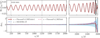
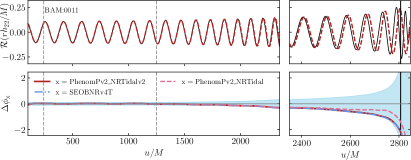
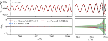
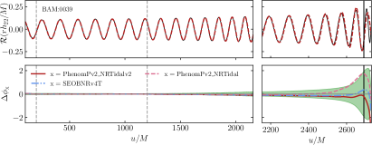
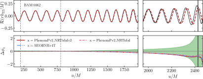
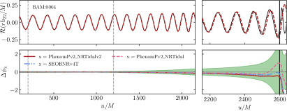
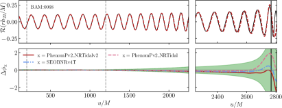
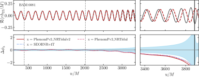
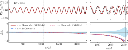
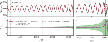
Figure 8: Top panel: Real part of the GW signal obtained from the NR data (black) and the IMRPhenomPv2_NRTidalv2 model (red dashed). Bottom panel: Phase difference between the NR data listed in Table 3 and the IMRPhenomPv2_NRTidalv2, IMRPhenomPv2_NRTidal, and SEOBNRv4T models; note that we discard the IMR-prefix for better visibility in the panel legends. The green shaded regions denote the errors computed using Richardson extrapolation and $u$ is the retarded time, while blue shaded regions present the phase difference between the two highest NR resolutions. The vertical dashed lines mark the alignment region while the solid vertical line marks the merger. See the main text for further details.

IV.1 Time domain comparison with NR simulations

As a first validation check, we compute the time domain phase difference between IMRPhenomPv2_NRTidalv2 and a selected set of NR data; see Table 3. All of the employed waveforms are publicly available in the CoRe database (www.computational-relativity.org Dietrich et al. (2018)). In addition to IMRPhenomPv2_NRTidalv2, we also present the phase difference with respect to SEOBNRv4T and IMRPhenomPv2_NRTidal in Fig. 8.

Waveform alignment: For comparison, we align all waveforms with respect to the NR data by minimizing the phase difference in the time interval $[t_{i},t_{f}]$

$$\mathcal{I}(\delta t,\delta\phi)=\int_{t_{i}}^{t_{f}}|\phi_{\rm NR}(t)-\phi_{\rm x}(t+\delta t)+\delta\phi|\,\text{d}t,$$ (30)

where $\rm x$ denotes the individual waveform approximant. The alignment windows are marked by vertical dashed lines in Fig. 8.

NR data uncertainty: For a quantitative comparison with respect to the NR data, we assign each dataset with an uncertainty, where we generally distinguish between (i) setups employing the high-order flux scheme of Bernuzzi and Dietrich (2016) for which clean convergence is found throughout the inspiral, and (ii) setups whose behavior is monotonic, but no clean convergence is present. For the setups employing the high-order flux scheme, we obtain a better phase estimate and an error measure (green shaded region) due to Richardson extrapolation Bernuzzi and Dietrich (2016); Dietrich et al. (2018); cf. Sec. II.2. Other configurations are marked by blue shaded regions. For these cases, the uncertainty due to numerical discretization is estimated by the difference between the two highest resolutions, which is not necessarily a conservative error estimate. For both scenarios, we also include an error measuring the effect of the finite radius extraction of the GW from the numerical domain. This error measure is obtained by computing the difference in the waveform’s phase with respect to different extraction radii; see e.g. Refs. Bernuzzi and Dietrich (2016); Dietrich and Hinderer (2017) for a more detailed discussion.

NRTidalv2 dephasing: Considering the performance of the NRTidalv2 approximation, we find that for all cases with reliable error measure (green shaded regions), the dephasing between the model and the NR data is well within the error estimate and never exceeds $1\ \rm rad$. The performance is comparable with the SEOBNRv4T model which is shown as a blue dashed-dotted line. Considering the difference with respect to IMRPhenomPv2_NRTidal, we find that as expected the new NRTidalv2 model is less attractive, which is caused by the slightly different behavior in the frequency range $\hat{\omega}\geq 0.05$.

For the NR setups which show no clear convergence throughout the inspiral, we find that for most cases the estimated uncertainty is larger than the phase difference between the NRTidalv2 and the NR data, the exceptions are BAM:0081 and BAM:0094. These setups are characterized by high mass ratios [BAM:0094 is to date the NR dataset with the largest simulated mass ratio ($q=2.1$)] and tidal deformabilities which are in tension with the observation of GW170817 Abbott et al. (2018).

Additional simulations with clean convergence for large mass ratios are needed to allow an overall improvement of BNS models in these regions of the parameter space (see Appendix B).

IV.2 Mismatch Computations with respect to EOB-NR hybrids

Table 4: BNS hybrid configurations. The columns describe: the name of the hybrid (CoRe database ID), the EOS, cf. Read et al. (2009), the NSs’ individual masses $M_{A,B}$, the stars’ dimensionless spins $\chi_{A,B}$, the stars’ compactnesses $C_{A,B}$, the tidal deformabilities of the stars $\Lambda_{A,B}$, the tidal deformability of the binary $\tilde{\Lambda}$, the effective dimensionless coupling constant $\kappa^{T}_{\rm eff}$, and the merger frequency $f_{\rm mrg}$.

Name	EOS	$M_{A}$ $[M_{\odot}]$	$M_{B}$ $[M_{\odot}]$	$\chi_{A}$	$\chi_{B}$	$C_{A}$	$C_{B}$	$\Lambda_{A}$	$\Lambda_{B}$	$\tilde{\Lambda}$	$\kappa^{T}_{\rm eff}$	$f_{\rm mrg}$ [Hz]
equal mass, non-spinning
CoRe:Hyb:0001	2B	1.3500	1.3500	0.000	0.000	0.205	0.205	127.5	127.5	127.5	23.9	2567
CoRe:Hyb:0002	SLy	1.3500	1.3500	0.000	0.000	0.174	0.174	392.1	392.1	392.1	73.5	2010
CoRe:Hyb:0003	H4	1.3717	1.3717	0.000	0.000	0.149	0.149	1013.4	1013.4	1013.4	190.0	1535
CoRe:Hyb:0004	MS1b	1.3500	1.3500	0.000	0.000	0.142	0.142	1536.7	1536.7	1536.7	288.1	1405
CoRe:Hyb:0005	MS1b	1.3750	1.3750	0.000	0.000	0.144	0.144	1389.4	1389.4	1389.4	260.5	1416
CoRe:Hyb:0006	SLy	1.3750	1.3750	0.000	0.000	0.178	0.178	347.3	347.3	347.3	65.1	1978
unequal mass, non-spinning
CoRe:Hyb:0007	MS1b	1.5000	1.0000	0.000	0.000	0.157	0.109	866.5	7041.6	2433.5	456.3	1113
CoRe:Hyb:0008	MS1b	1.6500	1.1000	0.000	0.000	0.171	0.118	505.2	4405.9	1490.1	279.4	1170
CoRe:Hyb:0009	MS1b	1.5278	1.2222	0.000	0.000	0.159	0.130	779.6	2583.2	1420.4	266.3	1301
CoRe:Hyb:0010	SLy	1.5000	1.0000	0.000	0.000	0.194	0.129	192.3	2315.0	720.0	135.0	1504
CoRe:Hyb:0011	SLy	1.5274	1.2222	0.000	0.000	0.198	0.157	167.5	732.2	365.6	68.6	1770
CoRe:Hyb:0012	SLy	1.6500	1.0979	0.000	0.000	0.215	0.142	93.6	1372.3	408.1	76.5	1592
equal mass, spinning
CoRe:Hyb:0013	H4	1.3726	1.3726	+0.141	+0.141	0.149	0.149	1009.1	1009.1	1009.1	189.2	1605
CoRe:Hyb:0014	MS1b	1.3504	1.3504	-0.099	-0.099	0.142	0.142	1534.5	1534.5	1534.5	287.7	1323
CoRe:Hyb:0015	MS1b	1.3504	1.3504	+0.099	+0.099	0.142	0.142	1534.5	1534.5	1534.5	287.7	1442
CoRe:Hyb:0016	MS1b	1.3509	1.3509	+0.149	+0.149	0.142	0.142	1531.8	1531.8	1531.8	287.2	1456
CoRe:Hyb:0017	SLy	1.3502	1.3502	+0.052	+0.052	0.174	0.174	392.0	392.0	392.0	73.5	2025
CoRe:Hyb:0018	SLy	1.3506	1.3506	+0.106	+0.106	0.174	0.174	391.0	391.0	391.0	73.5	2048

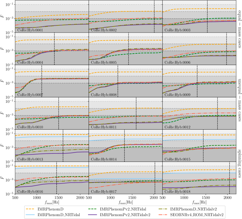
Figure 9: Mismatch with respect to the TEOBResumS-NR hybrids. We mark the merger frequency with a vertical dashed line. For CoRe:Hyb:0001 the merger happens at $2567\rm Hz$. The horizontal dashed lines mark mismatches of $10^{-3}$, $10^{-2}$, and $10^{-1}$.

To validate the new NRTidalv2 model, we compare our LALSuite implementation against a set of target waveforms combining TEOBResumS and NR data by computing the mismatch. Those waveforms have been constructed for Ref. Dietrich et al. (2019) and are publicly available under www.computational-relativity.org Dietrich et al. (2018). We refer to Dietrich et al. (2019) for further details. The main properties of these target waveforms are summarized in Table 4.

Mismatch computation: We compute the mismatch according to

$$\bar{F}=1-\max_{\phi_{c},t_{c}}\frac{(h_{1}(\phi_{c},t_{c})|h_{2})}{\sqrt{(h_{1}|h_{1})(h_{2}|h_{2})}}\,,$$ (31)

where $\phi_{c},t_{c}$ are an arbitrary phase and time shift. The noise-weighted overlap is given by

$$(h_{1}|h_{2})=4\Re\int_{f_{\rm min}}^{f_{\rm max}}\frac{\tilde{h}_{1}(f)\tilde{h}_{2}(f)}{S_{n}(f)}\,\text{d}f\ ,$$ (32)

where tildes denote the Fourier transform, $S_{n}(f)$ is the spectral density of the detector noise, and $f$ is the GW frequency (in the frequency domain). We used the Advanced LIGO zero-detuning, high-power (ZERO_DET_high_P) noise curve of adl for our analysis with a fixed $f_{\rm min}=30\,{\rm Hz}$ and a variable $f_{\rm max}$ ranging from 500 Hz up to the merger frequency ($f_{\rm mrg}$) reported in Table 4.

Mismatch with respect to hybrid waveforms: We compute the mismatch for $18$ TEOBResumS-NR hybrid waveforms (Table 4) against a range of different phenomenological models: IMRPhenomD Husa et al. (2016); Khan et al. (2016) (no tidal effects), IMRPhenomD_NRTidal (incorporating tidal effects using the NRTidal model of Dietrich et al. (2019) but no quadrupole-monopole self-spin terms), IMRPhenomPv2_NRTidal incorporating tidal effects using the NRTidal model of Dietrich et al. (2019) including quadrupole-monopole self-spin terms up to 3PN, and the new model IMRPhenomPv2_NRTidalv2. In addition, we include the new SEOBNRv4_ROM_NRTidalv2 and IMRPhenomD_NRTidalv2 approximants. We evaluate the waveform models at the parameters of the hybrids reported in Table 4 with an initial frequency of $30\,{\rm Hz}$.

Generally, we find that IMRPhenomPv2_NRTidalv2 performs as well or better than IMRPhenomPv2_NRTidal, except for 2 cases. For all configurations the mismatch stays below $5\times 10^{-3}$ even for maximum frequencies at or above the merger frequency. In addition, our comparisons show again that the inclusion of the quadrupole-monopole terms is important even for astrophysically reasonable spins—see Harry and Hinderer (2018); Dietrich et al. (2019); Samajdar and Dietrich (2019) for previous studies. In most cases the mismatches between the hybrids and IMRPhenomD_NRTidalv2 are marginally smaller compared to SEOBNRv4_ROM_NRTidalv2. Even less notable are the differences between IMRPhenomD_NRTidalv2 and IMRPhenomPv2_NRTidalv2 which are dominantly driven by the additional 3.5PN spin-spin and cubic-in-spin contributions in IMRPhenomPv2_NRTidalv2. The additional tidal amplitude corrections have almost a negligible effect; cf. the non-spinning configurations in Fig. 9.

Our comparison shows that the TEOBResumS-NR hybrids are well described by the new approximant and that no additional pathologies (in the low frequency regime) are introduced during recalibration.

IV.3 Cross validation against SEOBNRv4T

As a final check of the approximant, we compute the mismatch between the IMRPhenomPv2_NRTidalv2 and the SEOBNRv4T model for a number of randomly sampled configurations. We compare these mismatches with mismatches between IMRPhenomPv2 and IMRPhenomPv2_NRTidalv2 to give an impression of the importance of tidal effects. The match computation is restricted to the frequency interval of $f\in[40,2048]\ \rm Hz$. We have tested starting frequencies of $25\ \rm Hz$ and $30\ \rm Hz$ for a smaller number of cases and obtained smaller mismatches than for the $40\ \rm Hz$ initial frequency. Therefore, to save computational costs and to provide a conservative estimate, we use a minimum frequency of $40\ \rm Hz$.

IV.3.1 Non-spinning Configurations

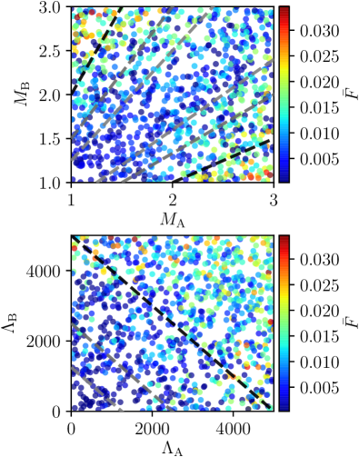
Figure 10: Mismatch between IMRPhenomPv2_NRTidalv2 and SEOBNRv4T. We consider $1000$ randomly distributed non-spinning configurations with $M_{A},M_{B}\in[1,3]\,M_{\odot}$ (here we relax our usual assumption that $M_{A}\geq M_{B}$) and $\Lambda_{A},\Lambda_{B}\in[0,5000]$. The mismatches are computed within the frequency interval $f\in[40,2048]\ \rm Hz$ and we use a sampling rate of $8192\ \rm Hz$. We mark in the top panel mass ratios of $1.25;1.5;2.0$ with diagonal gray, dark gray, black dashed lines, respectively. Similarly, $\Lambda_{A}+\Lambda_{B}=1250;2500;5000$ are marked in the bottom panel.

We start this analysis by considering non-spinning configurations. For this purpose, we select $1000$ samples with flat priors in $M_{A},M_{B}\in[1,3]\,M_{\odot}$ and $\Lambda_{A},\Lambda_{B}\in[0,5000]$. The final analysis is shown in Fig. 10, where we compare the IMRPhenomPv2_NRTidalv2 and SEOBNRv4T approximant. For non-spinning configurations the mismatches between IMRPhenomPv2_NRTidalv2 and SEOBNRv4T are below $0.034$ for our set of configurations. The largest difference is found for large mass ratios; cf. upper left and lower right corners of the top panel. For better visualization, we mark mass ratios of $q=1.25;1.5;2.0$ by diagonal gray, dark gray, and black lines, respectively. Restricting to mass ratios below $1.5$, we find a largest mismatch of $\bar{F}=0.024$

In addition, our analysis shows that for larger tidal deformabilities the mismatch between the two models tends to increase; cf. upper right corner of the right panel in Fig. 10. We mark in the plot $\Lambda_{A}+\Lambda_{B}=1250;2500;5000$ with gray, dark gray, and black lines. Restricting our analysis to $\Lambda_{A}+\Lambda_{B}<2500$ leads to a maximum mismatch of $\bar{F}=0.016$.

Overall, the average mismatch between IMRPhenomPv2_NRTidalv2 and SEOBNRv4T for our dataset is $0.009$. Interestingly, if we restrict our analysis to the more physical parameter space in which the more massive star has the smaller tidal deformability, the average mismatch decreases by roughly a factor of 2 to $0.0059$.

Consequently, we find for non-spinning configurations a good agreement between the tidal EOB model SEOBNRv4T and IMRPhenomPv2_NRTidalv2.

IV.3.2 Spinning Configurations

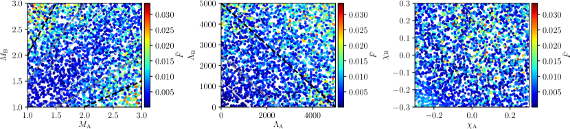
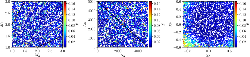
Figure 11: Mismatch between IMRPhenomPv2_NRTidalv2 and SEOBNRv4T. We consider randomly distributed configurations with $M_{A,B}\in[1,3]\,M_{\odot}$, $\Lambda_{A,B}\in[0,5000]$, and $\chi_{A,B}\in[-0.30,0.30]$, as well as $\chi_{A,B}\in[-0.70,0.70]$. The mismatches are computed within the frequency interval $f\in[40,2048]\ \rm Hz$ and a sampling rate of $8192\ \rm Hz$ is employed. We select $3000$ random samples for configurations with spins $\chi_{A,B}\in[-0.30,0.30]$ (top panels) and $3000$ samples for $\chi_{A,B}\in[-0.60,0.60]$ (bottom panels).

We further consider spinning configurations using flat priors $M_{A,B}\in[1,3]\,M_{\odot}$, $\Lambda_{A,B}\in[0,5000]$, and $\chi_{A,B}\in[-0.30,0.30]$ as well as $\chi_{A,B}\in[-0.60,0.60]$. For both prior choices we select $3000$ randomly distributed samples.

If we consider spins within $\chi_{A,B}\in[-0.30,0.30]$ (upper panels of Fig. 11), we find a maximum mismatch of $\bar{F}=0.034$, which is comparable with the non-spinning result presented before. Overall, the average mismatch of our $3000$ samples for spins within $\chi_{A,B}\in[-0.30,0.30]$ is $\bar{F}=0.0072$. For the same set of configurations, the average mismatch with respect to IMRPhenomPv2_NRTidal is $\bar{F}=0.0092$, i.e., $25\%$ larger. Furthermore, we find that, as for the non-spinning cases, the largest mismatches are obtained for configurations which have large mass ratios and large tidal deformabilities. If only spin magnitudes up to $|\chi_{A,B}|\leq 0.3$ are considered, we do not find a noticeable spin effect.

However, spin effects become important for large spin magnitudes. For spin magnitudes up to $0.6$, the largest mismatches between SEOBNRv4T and IMRPhenomPv2_NRTidalv2 are found for large anti-aligned spins, i.e., the lower left corner of the right-most bottom panel of Fig. 11. The maximum mismatch is ${\bar{F}=0.167}$ for our randomly chosen set of configurations.

Comparing average values, we find that while the average mismatch is $0.043$ between the original IMRPhenomPv2_NRTidal model and SEOBNRv4T, the average mismatch decreases to $0.021$ between the IMRPhenomPv2_NRTidalv2 model and SEOBNRv4T, i.e., much better agreement is found within this large region of the parameter space.

The disagreement between SEOBNRv4T and IMRPhenomPv2_NRTidalv2 for large anti-aligned spins needs further investigation and requires additional NR simulations in regions of the parameter space which are currently not covered. Note that for the largest anti-aligned spin, high-quality NR setups (CoRe:BAM:0062) the NSs have only a spin of $\chi_{A,B}=-0.10$. For this physical configuration, both waveform approximants (SEOBNRv4T and IMRPhenomPv2_NRTidalv2) describe the data within the estimated uncertainty.

V Summary

In this article we have presented our most recent update of the NRTidal model. The model gives a closed analytical expression for tidal effects during the BNS coalescence and can be added to an arbitrary BBH baseline approximant. We added the new NRTidalv2 approximant to IMRPhenomPv2 Hannam et al. (2014); Khan et al. (2016) to obtain a frequency-domain precessing BNS approximant as well as to the (frequency-domain) SEOBNRv4_ROM Bohé et al. (2017) and the IMRPhenomD Khan et al. (2016) approximants to allow an improved and fast modeling of spin-aligned systems.

Our main improvements in comparison to the initial NRTidal model are:

1. a recalibration of the tidal phase to improved NR data incorporating additional analytical knowledge for the low frequency limit;

2. the addition of a tidal amplitude correction to the model;

3. incorporation of higher order (3.5PN) quadrupole and octupole information to the spin sector of the model.

We also hope to further improve the NRTidalv2 model for higher mass ratios to allow an accurate description of high mass ratio systems. Such an extension requires additional high-quality NR simulations for a variety of different mass ratios.

An additional improvement would be the incorporation of the effect of $f$-mode resonances as recently computed in Refs. Andersson and Pnigouras (2019); Schmidt and Hinderer (2019), the incorporation of an updated precession dynamics as used in Khan et al. (2018), or the incorporation of higher modes London et al. (2018); Cotesta et al. (2018).

We have compared the IMRPhenomPv2_NRTidalv2 model with high resolution numerical relativity data and found agreement within the estimated uncertainty for all NR data with clear convergence. Overall, the performance of IMRPhenomPv2_NRTidalv2 is comparable with state-of-the-art tidal EOB models.

This accuracy was verified by the mismatch computation between IMRPhenomPv2_NRTidalv2 and TEOBResumS-NR hybrid waveforms, for which mismatches are well below $5\times 10^{-3}$.

We concluded the performance test of the model with a mismatch computation with respect to the tidal EOB model SEOBNRv4T. For non-spinning cases (or cases with small spins as employed in the low spin prior of the LVC analysis) the mismatch computed from a starting frequency of $40\ \rm Hz$ never exceeds $\bar{F}\approx 0.034$ for $M_{A,B}\in[1,3]\,M_{\odot}$ and $\Lambda_{A,B}\in[0,5000]$. Considering spinning setups ($\chi_{A,B}\in[-0.6,0.6]$), the mismatch increases to a maximum of $\bar{F}=0.164$.

Appendix A Alternative formulation of a tidal amplitude correction

A.1 Tidal amplitude corrections in the time domain

As in the frequency domain, the BNS waveform time domain amplitude can be obtained by augmenting existing BBH-models with additional tidal corrections $A_{\rm T}$, i.e.,

$$A_{\rm BNS}=A_{\rm BBH}+A_{\rm T}.$$ (33)

Refs. Damour et al. (2012); Banihashemi and Vines (2018) present the tidal amplitude corrections for the leading and next-to-leading order

$$\begin{split}A_{\rm T}&=\frac{8M\nu}{D_{L}}x\sqrt{\frac{\pi}{5}}\biggl{\{}\Lambda_{A}X_{A}^{4}x^{5}\biggl{[}3(1+2X_{B})\\ &\quad+\frac{63-15X_{B}-205X_{B}^{2}-45X_{B}^{3}}{14}x+\mathcal{O}(x^{3/2})\biggr{]}\\ &\quad+[A\leftrightarrow B]\biggr{\}}.\end{split}$$ (34)

While Eq. (34) describes the tidal amplitude corrections for small frequencies, it loses validity close to the moment of merger. For extreme cases, i.e., stiff EOSs and low NS masses, the additional amplitude corrections can become larger than $A_{\rm BBH}$ causing the overall amplitude to be negative. Thus, a further calibration to NR or EOB data is required. We will employ the quasi-universal relations, which allow an EOS-independent description of important quantities at the moment of merger (merger frequency, merger amplitude, reduced binding energy, specific orbital angular momentum, and GW luminosity) Bernuzzi et al. (2014); Takami et al. (2015); Dietrich (2016); Zappa et al. (2018). As shown in Fig. 6.7 of Ref. Dietrich (2016), the GW amplitude at the merger follows a quasi-universal relation as a function of the tidal coupling constant

$$\kappa^{T}_{2}=2\left[\frac{X_{B}}{X_{A}}\left(\frac{X_{A}}{C_{A}}\right)^{5}k^{A}_{2}+\frac{X_{A}}{X_{B}}\left(\frac{X_{B}}{C_{B}}\right)^{5}k^{B}_{2}\right],$$ (35)

namely,

$$D_{L}A^{\rm mrg}/(\nu M)=$$

$$1.6498\frac{1+2.5603\cdot 10^{-2}\kappa_{2}^{T}-1.024\cdot 10^{-5}(\kappa_{2}^{T})^{2}}{1+4.7278\cdot 10^{-2}\kappa^{T}_{2}}.$$ (36)

We note that a straightforward extension of Eq. (36) [Eq. (6.15d) of Ref. Dietrich (2016)], would be the incorporation of a larger number of NR simulations as publicly available under www.computational-relativity.org, Ref. Dietrich et al. (2018). However, we postpone this to future work Zappa et al. , in which a more general discussion about quasi-universal relations during the BNS coalescence will be given.

To incorporate Eq. (36) in Eq. (34), we extend the analytical knowledge with an additional, unknown higher order PN-term and define the NRTidal amplitude correction as

$$A_{\rm T}^{\rm NRTidal}=\frac{8M\nu}{D_{L}}x\sqrt{\frac{\pi}{5}}\left(\hat{c}_{A}\kappa_{A}x^{5}\frac{1+\hat{c}_{1}^{A}x}{1+\hat{d}x}+\hat{c}_{B}\kappa_{B}x^{5}\frac{1+\hat{c}_{1}^{B}x}{1+\hat{d}x}\right),$$ (37)

where the individual terms $\hat{c}_{A},\hat{c}_{1}^{A},\hat{c}_{B},\hat{c}_{1}^{B}$ can be obtianed from Eq. (34) once we express $\Lambda_{A,B}$ in terms of $\kappa_{A,B}$.

Enforcing

$$A^{\rm mrg}(x^{\rm mrg})=A_{\rm BBH}(x^{\rm mrg})+A_{\rm T}^{\rm NRTidal}(x^{\rm mrg})$$ (38)

gives us the unknown parameter $d$ according to

$$d =\left\{\frac{8M\nu x^{5}}{D_{L}\ \Delta A}\sqrt{\frac{\pi}{5}}\left[\hat{c}_{A}\kappa_{A}\left(1+\hat{c}_{1}^{A}x\right)\right.\right.$$

$$\quad+\left.\left.\hat{c}_{B}\kappa_{B}\left(1+\hat{c}_{1}^{B}x\right)\right]-\frac{1}{x}\right\}_{x=x^{\rm mrg}}$$ (39)

with $\Delta A=A^{\rm mrg}(x^{\rm mrg})-A_{\rm BBH}(x^{\rm mrg})$.

We note that although the outlined approach has been tested for a selected number of cases, we did not implemented it in LALSuite due to the large computational costs inherent to time domain waveform approximants.

A.2 Frequency domain amplitude corrections by SPA

In addition to the frequency domain amplitude correction presented in the main text, we also want to present a possible alternative way to augment the frequency domain binary black hole amplitude with tidal correction. For this purpose we use the SPA to obtain the frequency-domain amplitude from Eq. (37). Following the SPA approach,

$$\tilde{A}=\frac{1}{2}\sqrt{\frac{2\pi}{\ddot{\phi}}}A,$$ (40)

where $\ddot{\phi}$ refers to the second time derivative of $\phi$.

Using Eq. (16) [see also Eq. (14) in Damour et al. (2012); note that the published version is missing an equals sign], Eq. (40) can be rewritten as

$$\tilde{A}=A\sqrt{\frac{\pi}{2}}\ \sqrt{\frac{\text{d}^{2}\psi}{\text{d}\hat{\omega}^{2}}}.$$ (41)

Inserting $A=A_{\rm BBH}+A_{\rm T}$ and $\psi=\psi_{\rm BBH}+\psi_{T}$ leads to

$$\tilde{A}=(A_{\rm BBH}+A_{\rm T})\sqrt{\frac{\pi}{2}}\ \sqrt{\frac{\text{d}^{2}\psi_{\rm BBH}}{\text{d}\hat{\omega}^{2}}+\frac{\text{d}^{2}\psi_{\rm T}}{\text{d}\hat{\omega}^{2}}}.$$ (42)

Treating the tidal phase correction as a small change of the underlying BBH waveform, we rewrite the expression as

$$\tilde{A}=(A_{\rm BBH}+A_{\rm T})\sqrt{\frac{\pi}{2}}\ \sqrt{\frac{\text{d}^{2}\psi_{\rm BBH}}{\text{d}\hat{\omega}^{2}}}\sqrt{1+\underbrace{\frac{\text{d}^{2}\psi_{\rm T}}{\text{d}\hat{\omega}^{2}}\bigg{/}\frac{\text{d}^{2}\psi_{\rm BBH}}{\text{d}\hat{\omega}^{2}}}_{\epsilon}}.$$ (43)

Linearizing in $\epsilon=\mathcal{O}(\kappa)$ and neglecting terms proportional to $\kappa^{2}$ [noting that $A_{\rm T}=\mathcal{O}(\kappa)$] leads to

$$\tilde{A}=\underbrace{A_{\rm BBH}\sqrt{\frac{\pi}{2}}\ \sqrt{\frac{\text{d}^{2}\psi_{\rm BBH}}{\text{d}\hat{\omega}^{2}}}}_{\tilde{A}_{\rm BBH}}\left(1+\frac{\epsilon}{2}\right)+A_{\rm T}\underbrace{\sqrt{\frac{\pi}{2}}\ \sqrt{\frac{\text{d}^{2}\psi_{\rm BBH}}{\text{d}\hat{\omega}^{2}}}}_{\tilde{A}_{\rm BBH}/A_{\rm BBH}}.$$ (44)

Thus, the final expression is given as

$$\frac{\tilde{A}}{\tilde{A}_{\rm BBH}}=1+\frac{A_{\rm T}}{A_{\rm BBH}}+\frac{1}{2}\frac{\text{d}^{2}\psi_{\rm T}}{\text{d}\hat{\omega}^{2}}\bigg{/}\frac{\text{d}^{2}\psi_{\rm BBH}}{\text{d}\hat{\omega}^{2}}.$$ (45)

The approach outlined in this appendix, i.e., Eq. (45), leads to much larger computational cost than the Padé approximant [Eq. (24)], which is why we chose the easier and more straightforward implementation shown in the main body of the paper. However, this additional approach might become relevant for a potential improvement/extension in the future.

Appendix B Extension of the NRTidal phase incorporating additional mass ratio dependence

We now outline a possible extension of the NRTidalv2 model which incorporates additional analytically known mass-ratio dependence. Since we do not find such an extension to perform better in our tests and to reduce computational costs, we limited the mass ratio dependence in the tidal phase simply to the prefactor $\propto\kappa_{\rm eff}^{T}/\nu$ in the current implementation of the model.

However, it is possible to recast Eq. (17) as

$$\psi_{\rm T}(x)=-\kappa_{A}c^{A}_{0}x^{5/2}\tilde{P}_{\rm NRTidal}^{A}(x)-\kappa_{B}c^{B}_{0}x^{5/2}\tilde{P}_{\rm NRTidal}^{B}(x)$$ (46)

with $c_{0}^{A}=-\frac{3}{16X_{A}X_{B}}\left(12+\frac{X_{A}}{X_{B}}\right)$ (and similarly for $c_{0}^{B}$).

The individual Padé approximants $\tilde{P}_{\rm NRTidal}^{A}(x)$, $\tilde{P}_{\rm NRTidal}^{B}(x)$ are similar to Eq. (18) together with the constraints in Eqs. (19), but the known PN coefficients $\tilde{c}_{1}^{A,B},\tilde{c}_{3/2}^{A,B},\tilde{c}_{2}^{A,B},\tilde{c}_{5/2}^{A,B}$ have a mass ratio dependence as given in Ref. Damour et al. (2012).

Due to the limited set of high-quality NR data, the fitting coefficients in Eqs. (20) ($\tilde{d}_{1},\tilde{d}_{2},\tilde{n}_{5/2},\tilde{n}_{3}$) can only be determined for the equal mass case.

We find that while such a choice of the coefficients leads to a correct mass ratio dependence for the low frequency limit, the higher frequency phase is described worse compared to the NRTidalv2 approximation given in the main text. We suggest that this is caused by the inconsistency introduced by adding the mass-ratio dependence in only some of the Padé coefficients.

References

- Abbott et al. (2017) B. P. Abbott et al. (LIGO Scientific Collaboration and Virgo Collaboration), Phys. Rev. Lett., 119, 161101 (2017a), arXiv:1710.05832 [gr-qc] .
- Abbott et al. (2017) B. P. Abbott et al. (LIGO Scientific Collaboration, Virgo Collaboration, Fermi-GBM, and INTEGRAL), Astrophys. J. Lett., 848, L13 (2017b), arXiv:1710.05834 [astro-ph.HE] .
- Abbott et al. (2017) B. P. Abbott et al. (LIGO Scientific Collaboration, Virgo Collaboration, et al.), Astrophys. J. Lett., 848, L12 (2017c), arXiv:1710.05833 [astro-ph.HE] .
- Tanaka et al. (2017) M. Tanaka et al., Publ. Astron. Soc. Jap., 69, 102 (2017), arXiv:1710.05850 [astro-ph.HE] .
- Nicholl et al. (2017) M. Nicholl et al., Astrophys. J. Lett., 848, L18 (2017), arXiv:1710.05456 [astro-ph.HE] .
- Tanvir et al. (2017) N. R. Tanvir et al., Astrophys. J. Lett., 848, L27 (2017), arXiv:1710.05455 [astro-ph.HE] .
- Perego et al. (2017) A. Perego, D. Radice, and S. Bernuzzi, Astrophys. J. Lett., 850, L37 (2017), arXiv:1711.03982 [astro-ph.HE] .
- Waxman et al. (2018) E. Waxman, E. O. Ofek, D. Kushnir, and A. Gal-Yam, Mon. Not. R. Astron. Soc., 481, 3423 (2018), arXiv:1711.09638 [astro-ph.HE] .
- Metzger et al. (2018) B. D. Metzger, T. A. Thompson, and E. Quataert, Astrophys. J., 856, 101 (2018), arXiv:1801.04286 [astro-ph.HE] .
- Abbott et al. (2019) B. P. Abbott et al. (LIGO Scientific Collaboration and Virgo Collaboration), Phys. Rev. X, 9, 011001 (2019a), arXiv:1805.11579 [gr-qc] .
- Kawaguchi et al. (2018) K. Kawaguchi, M. Shibata, and M. Tanaka, Astrophys. J. Lett., 865, L21 (2018a), arXiv:1806.04088 [astro-ph.HE] .
- Hinderer et al. (2018) T. Hinderer et al., (2018), arXiv:1808.03836 [astro-ph.HE] .
- Coughlin et al. (2018) M. W. Coughlin, T. Dietrich, B. Margalit, and B. D. Metzger, (2018), arXiv:1812.04803 [astro-ph.HE] .
- Coughlin and Dietrich (2019) M. W. Coughlin and T. Dietrich, (2019), arXiv:1901.06052 [astro-ph.HE] .
- Siegel (2019) D. M. Siegel, (2019), arXiv:1901.09044 [astro-ph.HE] .
- Abbott et al. (2018) B. P. Abbott et al. (KAGRA Collaboration, LIGO Scientific Collaboration, and Virgo Collaboration), Living Rev. Relativity, 21, 3 (2018a), arXiv:1304.0670 [gr-qc] .
- Veitch et al. (2015) J. Veitch et al., Phys. Rev. D, 91, 042003 (2015), arXiv:1409.7215 [gr-qc] .
- Damour et al. (2012) T. Damour, A. Nagar, and L. Villain, Phys. Rev. D, 85, 123007 (2012), arXiv:1203.4352 [gr-qc] .
- Pani et al. (2018) P. Pani, L. Gualtieri, T. Abdelsalhin, and X. Jiménez-Forteza, Phys. Rev. D, 98, 124023 (2018), arXiv:1810.01094 [gr-qc] .
- Banihashemi and Vines (2018) B. Banihashemi and J. Vines, (2018), arXiv:1805.07266 [gr-qc] .
- Abdelsalhin et al. (2018) T. Abdelsalhin, L. Gualtieri, and P. Pani, Phys. Rev. D, 98, 104046 (2018), arXiv:1805.01487 [gr-qc] .
- Landry (2018) P. Landry, (2018), arXiv:1805.01882 [gr-qc] .
- Jiménez Forteza et al. (2018) X. Jiménez Forteza, T. Abdelsalhin, P. Pani, and L. Gualtieri, Phys. Rev. D, 98, 124014 (2018), arXiv:1807.08016 [gr-qc] .
- Hotokezaka et al. (2015) K. Hotokezaka, K. Kyutoku, H. Okawa, and M. Shibata, Phys. Rev. D, 91, 064060 (2015), arXiv:1502.03457 [gr-qc] .
- Bernuzzi and Dietrich (2016) S. Bernuzzi and T. Dietrich, Phys. Rev. D, 94, 064062 (2016), arXiv:1604.07999 [gr-qc] .
- Kiuchi et al. (2017) K. Kiuchi, K. Kawaguchi, K. Kyutoku, Y. Sekiguchi, M. Shibata, and K. Taniguchi, Phys. Rev. D, 96, 084060 (2017), arXiv:1708.08926 [astro-ph.HE] .
- Dietrich et al. (2018) T. Dietrich, S. Bernuzzi, B. Brügmann, and W. Tichy, in Proceedings, 26th Euromicro International Conference on Parallel, Distributed and Network-based Processing (PDP 2018): Cambridge, UK, March 21-23, 2018 (2018) pp. 682–689, arXiv:1803.07965 [gr-qc] .
- Dietrich et al. (2018) T. Dietrich, D. Radice, S. Bernuzzi, F. Zappa, A. Perego, B. Brügmann, S. V. Chaurasia, R. Dudi, W. Tichy, and M. Ujevic, Classical Quantum Gravity, 35, 24LT01 (2018b), arXiv:1806.01625 [gr-qc] .
- Foucart et al. (2019) F. Foucart et al., Phys. Rev. D, 99, 044008 (2019), arXiv:1812.06988 [gr-qc] .
- Bernuzzi et al. (2012) S. Bernuzzi, A. Nagar, M. Thierfelder, and B. Brügmann, Phys. Rev. D, 86, 044030 (2012), arXiv:1205.3403 [gr-qc] .
- Favata (2014) M. Favata, Phys. Rev. Lett., 112, 101101 (2014), arXiv:1310.8288 [gr-qc] .
- Wade et al. (2014) L. Wade, J. D. E. Creighton, E. Ochsner, B. D. Lackey, B. F. Farr, T. B. Littenberg, and V. Raymond, Phys. Rev. D, 89, 103012 (2014), arXiv:1402.5156 [gr-qc] .
- Hotokezaka et al. (2016) K. Hotokezaka, K. Kyutoku, Y.-i. Sekiguchi, and M. Shibata, Phys. Rev. D, 93, 064082 (2016), arXiv:1603.01286 [gr-qc] .
- Dietrich et al. (2019) T. Dietrich et al., Phys. Rev. D, 99, 024029 (2019), arXiv:1804.02235 [gr-qc] .
- Dudi et al. (2018) R. Dudi, F. Pannarale, T. Dietrich, M. Hannam, S. Bernuzzi, F. Ohme, and B. Brügmann, Phys. Rev. D, 98, 084061 (2018), arXiv:1808.09749 [gr-qc] .
- Samajdar and Dietrich (2018) A. Samajdar and T. Dietrich, Phys. Rev. D, 98, 124030 (2018), arXiv:1810.03936 [gr-qc] .
- Bernuzzi et al. (2015) S. Bernuzzi, A. Nagar, T. Dietrich, and T. Damour, Phys. Rev. Lett., 114, 161103 (2015), arXiv:1412.4553 [gr-qc] .
- Hinderer et al. (2016) T. Hinderer et al., Phys. Rev. Lett., 116, 181101 (2016), arXiv:1602.00599 [gr-qc] .
- Steinhoff et al. (2016) J. Steinhoff, T. Hinderer, A. Buonanno, and A. Taracchini, Phys. Rev. D, 94, 104028 (2016), arXiv:1608.01907 [gr-qc] .
- Nagar et al. (2018) A. Nagar et al., Phys. Rev. D, 98, 104052 (2018), arXiv:1806.01772 [gr-qc] .
- Nagar and Rettegno (2019) A. Nagar and P. Rettegno, Phys. Rev. D, 99, 021501(R) (2019), arXiv:1805.03891 [gr-qc] .
- Akcay et al. (2019) S. Akcay, S. Bernuzzi, F. Messina, A. Nagar, N. Ortiz, and P. Rettegno, Phys. Rev. D, 99, 044051 (2019), arXiv:1812.02744 [gr-qc] .
- Nagar et al. (2019) A. Nagar, F. Messina, P. Rettegno, D. Bini, T. Damour, A. Geralico, S. Akcay, and S. Bernuzzi, Phys. Rev. D, 99, 044007 (2019), arXiv:1812.07923 [gr-qc] .
- Buonanno and Damour (1999) A. Buonanno and T. Damour, Phys. Rev. D, 59, 084006 (1999), arXiv:gr-qc/9811091 .
- Damour and Nagar (2010) T. Damour and A. Nagar, Phys. Rev. D, 81, 084016 (2010), arXiv:0911.5041 [gr-qc] .
- Dietrich and Hinderer (2017) T. Dietrich and T. Hinderer, Phys. Rev. D, 95, 124006 (2017), arXiv:1702.02053 [gr-qc] .
- Lackey et al. (2017) B. D. Lackey, S. Bernuzzi, C. R. Galley, J. Meidam, and C. Van Den Broeck, Phys. Rev. D, 95, 104036 (2017), arXiv:1610.04742 [gr-qc] .
- Lackey et al. (2019) B. D. Lackey, M. Pürrer, A. Taracchini, and S. Marsat, Phys. Rev. D, 100, 024002 (2019), arXiv:1812.08643 [gr-qc] .
- Lackey et al. (2014) B. D. Lackey, K. Kyutoku, M. Shibata, P. R. Brady, and J. L. Friedman, Phys. Rev. D, 89, 043009 (2014), arXiv:1303.6298 [gr-qc] .
- Pannarale et al. (2013) F. Pannarale, E. Berti, K. Kyutoku, and M. Shibata, Phys. Rev. D, 88, 084011 (2013), arXiv:1307.5111 [gr-qc] .
- Barkett et al. (2016) K. Barkett et al., Phys. Rev. D, 93, 044064 (2016), arXiv:1509.05782 [gr-qc] .
- Lange et al. (2017) J. Lange et al., Phys. Rev. D, 96, 104041 (2017), arXiv:1705.09833 [gr-qc] .
- Lange et al. (2018) J. Lange, R. O’Shaughnessy, and M. Rizzo, (2018), arXiv:1805.10457 [gr-qc] .
- Dietrich et al. (2017) T. Dietrich, S. Bernuzzi, and W. Tichy, Phys. Rev. D, 96, 121501(R) (2017), arXiv:1706.02969 [gr-qc] .
- LIGO Scientific Collaboration and Virgo Collaboration (2018) LIGO Scientific Collaboration and Virgo Collaboration, “LALSuite software,” (2018).
- Abbott et al. (2018) B. P. Abbott et al. (LIGO Scientific Collaboration and Virgo Collaboration), Phys. Rev. Lett., 121, 161101 (2018b), arXiv:1805.11581 [gr-qc] .
- Abbott et al. (2018) B. P. Abbott et al. (LIGO Scientific Collaboration and Virgo Collaboration), (2018c), arXiv:1811.12907 [astro-ph.HE] .
- Abbott et al. (2019) B. P. Abbott et al. (LIGO Scientific Collaboration and Virgo Collaboration), Phys. Rev. Lett., 123, 011102 (2019b), arXiv:1811.00364 [gr-qc] .
- Dai et al. (2018) L. Dai, T. Venumadhav, and B. Zackay, (2018), arXiv:1806.08793 [gr-qc] .
- Radice and Dai (2019) D. Radice and L. Dai, Eur. Phys. J. A, 55, 50 (2019), arXiv:1810.12917 [astro-ph.HE] .
- Kawaguchi et al. (2018) K. Kawaguchi, K. Kiuchi, K. Kyutoku, Y. Sekiguchi, M. Shibata, and K. Taniguchi, Phys. Rev. D, 97, 044044 (2018b), arXiv:1802.06518 [gr-qc] .
- Marsat (2015) S. Marsat, Classical Quantum Gravity, 32, 085008 (2015), arXiv:1411.4118 [gr-qc] .
- Bohé et al. (2015) A. Bohé, G. Faye, S. Marsat, and E. K. Porter, Classical Quantum Gravity, 32, 195010 (2015), arXiv:1501.01529 [gr-qc] .
- Krishnendu et al. (2017) N. V. Krishnendu, K. G. Arun, and C. K. Mishra, Phys. Rev. Lett., 119, 091101 (2017), arXiv:1701.06318 [gr-qc] .
- Flanagan and Hinderer (2008) É. É. Flanagan and T. Hinderer, Phys. Rev. D, 77, 021502(R) (2008), arXiv:0709.1915 [astro-ph] .
- Stovall et al. (2018) K. Stovall et al., Astrophys. J. Lett., 854, L22 (2018), arXiv:1802.01707 [astro-ph.HE] .
- Kumar and Landry (2019) B. Kumar and P. Landry, Phys. Rev. D, 99, 123026 (2019), arXiv:1902.04557 [gr-qc] .
- Read et al. (2009) J. S. Read, B. D. Lackey, B. J. Owen, and J. L. Friedman, Phys. Rev. D, 79, 124032 (2009), arXiv:0812.2163 [astro-ph] .
- Bauswein et al. (2017) A. Bauswein, O. Just, H.-T. Janka, and N. Stergioulas, Astrophys. J. Lett., 850, L34 (2017), arXiv:1710.06843 [astro-ph.HE] .
- Most et al. (2018) E. R. Most, L. R. Weih, L. Rezzolla, and J. Schaffner-Bielich, Phys. Rev. Lett., 120, 261103 (2018), arXiv:1803.00549 [gr-qc] .
- Cromartie et al. (2019) H. T. Cromartie et al., (2019), arXiv:1904.06759 [astro-ph.HE] .
- Brügmann et al. (2008) B. Brügmann, J. A. González, M. Hannam, S. Husa, U. Sperhake, and W. Tichy, Phys. Rev. D, 77, 024027 (2008), arXiv:gr-qc/0610128 [gr-qc] .
- Thierfelder et al. (2011) M. Thierfelder, S. Bernuzzi, and B. Brügmann, Phys. Rev. D, 84, 044012 (2011), arXiv:1104.4751 [gr-qc] .
- Dietrich et al. (2015) T. Dietrich, S. Bernuzzi, M. Ujevic, and B. Brügmann, Phys. Rev. D, 91, 124041 (2015), arXiv:1504.01266 [gr-qc] .
- (75) http://www.black-holes.org/SpEC.html, SpEC - Spectral Einstein Code.
- Mroué et al. (2013) A. H. Mroué et al., Phys. Rev. Lett., 111, 241104 (2013), arXiv:1304.6077 [gr-qc] .
- Blackman et al. (2015) J. Blackman, S. E. Field, C. R. Galley, B. Szilágyi, M. A. Scheel, M. Tiglio, and D. A. Hemberger, Phys. Rev. Lett., 115, 121102 (2015), arXiv:1502.07758 [gr-qc] .
- Hannam et al. (2014) M. Hannam, P. Schmidt, A. Bohé, L. Haegel, S. Husa, F. Ohme, G. Pratten, and M. Pürrer, Phys. Rev. Lett., 113, 151101 (2014), arXiv:1308.3271 [gr-qc] .
- Khan et al. (2016) S. Khan, S. Husa, M. Hannam, F. Ohme, M. Pürrer, X. Jiménez Forteza, and A. Bohé, Phys. Rev. D, 93, 044007 (2016), arXiv:1508.07253 [gr-qc] .
- Bohé et al. (2017) A. Bohé et al., Phys. Rev. D, 95, 044028 (2017), arXiv:1611.03703 [gr-qc] .
- Pürrer (2014) M. Pürrer, Classical Quantum Gravity, 31, 195010 (2014), arXiv:1402.4146 [gr-qc] .
- Pürrer (2016) M. Pürrer, Phys. Rev. D, 93, 064041 (2016), arXiv:1512.02248 [gr-qc] .
- Damour (1983) T. Damour, “Gravitational radiation and the motion of compact bodies, in Gravitational Radiation, edited by N. Deruelle and T. Piran,” (North-Holland, Amsterdam, 1983, 1983) pp. 59–144.
- Hinderer (2008) T. Hinderer, Astrophys. J., 677, 1216 (2008), arXiv:0711.2420 [astro-ph] .
- Damour and Nagar (2009) T. Damour and A. Nagar, Phys. Rev. D, 80, 084035 (2009), arXiv:0906.0096 [gr-qc] .
- Binnington and Poisson (2009) T. Binnington and E. Poisson, Phys. Rev. D, 80, 084018 (2009), arXiv:0906.1366 [gr-qc] .
- McKechan et al. (2010) D. J. A. McKechan, C. Robinson, and B. S. Sathyaprakash, Gravitational waves. Proceedings, 8th Edoardo Amaldi Conference, Amaldi 8, New York, USA, June 22-26, 2009, Classical Quantum Gravity, 27, 084020 (2010), arXiv:1003.2939 [gr-qc] .
- Pappas and Apostolatos (2014) G. Pappas and T. A. Apostolatos, Phys. Rev. Lett., 112, 121101 (2014), arXiv:1311.5508 [gr-qc] .
- Yagi et al. (2014) K. Yagi, K. Kyutoku, G. Pappas, N. Yunes, and T. A. Apostolatos, Phys. Rev. D, 89, 124013 (2014), arXiv:1403.6243 [gr-qc] .
- Mishra et al. (2016) C. K. Mishra, A. Kela, K. G. Arun, and G. Faye, Phys. Rev. D, 93, 084054 (2016), arXiv:1601.05588 [gr-qc] .
- Blanchet (2014) L. Blanchet, Living Rev. Relativity, 17, 2 (2014), arXiv:1310.1528 [gr-qc] .
- Yagi and Yunes (2017) K. Yagi and N. Yunes, Phys. Rep., 681, 1 (2017), arXiv:1608.02582 [gr-qc] .
- Kidder (1995) L. E. Kidder, Phys. Rev. D, 52, 821 (1995), arXiv:gr-qc/9506022 [gr-qc] .
- Apostolatos et al. (1994) T. A. Apostolatos, C. Cutler, G. J. Sussman, and K. S. Thorne, Phys. Rev. D, 49, 6274 (1994).
- Buonanno et al. (2003) A. Buonanno, Y.-b. Chen, and M. Vallisneri, Phys. Rev. D, 67, 104025 (2003), 74, 029904(E) (2006), arXiv:gr-qc/0211087 [gr-qc] .
- Schmidt et al. (2011) P. Schmidt, M. Hannam, S. Husa, and P. Ajith, Phys. Rev. D, 84, 024046 (2011), arXiv:1012.2879 [gr-qc] .
- Schmidt et al. (2012) P. Schmidt, M. Hannam, and S. Husa, Phys. Rev. D, 86, 104063 (2012), arXiv:1207.3088 [gr-qc] .
- Schmidt et al. (2015) P. Schmidt, F. Ohme, and M. Hannam, Phys. Rev. D, 91, 024043 (2015), arXiv:1408.1810 [gr-qc] .
- (99) Advanced LIGO anticipated sensitivity curves, LIGO Document T0900288-v3, https://dcc.ligo.org/LIGO-T0900288/public.
- (100) Updated Advanced LIGO sensitivity design curve, LIGO Document T1800044-v5, https://dcc.ligo.org/LIGO-T1800044/public.
- Husa et al. (2016) S. Husa, S. Khan, M. Hannam, M. Pürrer, F. Ohme, X. Jiménez Forteza, and A. Bohé, Phys. Rev. D, 93, 044006 (2016), arXiv:1508.07250 [gr-qc] .
- Harry and Hinderer (2018) I. Harry and T. Hinderer, Classical Quantum Gravity, 35, 145010 (2018), arXiv:1801.09972 [gr-qc] .
- Samajdar and Dietrich (2019) A. Samajdar and T. Dietrich, (2019), arXiv:1905.03118 [gr-qc] .
- Chatziioannou et al. (2015) K. Chatziioannou, K. Yagi, A. Klein, N. Cornish, and N. Yunes, Phys. Rev. D, 92, 104008 (2015), arXiv:1508.02062 [gr-qc] .
- Sieniawska et al. (2019) M. Sieniawska, W. Turczanski, M. Bejger, and J. L. Zdunik, Astron. Astrophys., 622, A174 (2019), arXiv:1807.11581 [astro-ph.HE] .
- Han and Steiner (2019) S. Han and A. W. Steiner, Phys. Rev. D, 99, 083014 (2019), arXiv:1810.10967 [nucl-th] .
- Andersson and Pnigouras (2019) N. Andersson and P. Pnigouras, (2019), arXiv:1905.00012 [gr-qc] .
- Schmidt and Hinderer (2019) P. Schmidt and T. Hinderer, (2019), arXiv:1905.00818 [gr-qc] .
- Khan et al. (2018) S. Khan, K. Chatziioannou, M. Hannam, and F. Ohme, (2018), arXiv:1809.10113 [gr-qc] .
- London et al. (2018) L. London, S. Khan, E. Fauchon-Jones, X. Jiménez-Forteza, M. Hannam, S. Husa, C. Kalaghatgi, F. Ohme, and F. Pannarale, Phys. Rev. Lett., 120, 161102 (2018), arXiv:1708.00404 [gr-qc] .
- Cotesta et al. (2018) R. Cotesta, A. Buonanno, A. Bohé, A. Taracchini, I. Hinder, and S. Ossokine, Phys. Rev. D, 98, 084028 (2018), arXiv:1803.10701 [gr-qc] .
- Bernuzzi et al. (2014) S. Bernuzzi, A. Nagar, S. Balmelli, T. Dietrich, and M. Ujevic, Phys. Rev. Lett., 112, 201101 (2014), arXiv:1402.6244 [gr-qc] .
- Takami et al. (2015) K. Takami, L. Rezzolla, and L. Baiotti, Phys. Rev. D, 91, 064001 (2015), arXiv:1412.3240 [gr-qc] .
- Dietrich (2016) T. Dietrich, Binary neutron star merger simulations, Ph.D. thesis, Jena (2016), dissertation, Friedrich-Schiller-Universität Jena, 2016.
- Zappa et al. (2018) F. Zappa, S. Bernuzzi, D. Radice, A. Perego, and T. Dietrich, Phys. Rev. Lett., 120, 111101 (2018), arXiv:1712.04267 [gr-qc] .
- (116) F. Zappa et al., (in preparation).