Can Graph Neural Networks Go “Online”? An Analysis of Pretraining and Inference

Abstract

Large-scale graph data in real-world applications is often not static but dynamic, i. e., new nodes and edges appear over time. Current graph convolution approaches are promising, especially, when all the graph’s nodes and edges are available during training. When unseen nodes and edges are inserted after training, it is not yet evaluated whether up-training or re-training from scratch is preferable. We construct an experimental setup, in which we insert previously unseen nodes and edges after training and conduct a limited amount of inference epochs. In this setup, we compare adapting pretrained graph neural networks against retraining from scratch. Our results show that pretrained models yield high accuracy scores on the unseen nodes and that pretraining is preferable over retraining from scratch. Our experiments represent a first step to evaluate and develop truly online variants of graph neural networks.

1 Introduction

Recent advances in graph neural networks yield promising results. Various methods have recently emerged for applying neural networks to graph-structured data (Bruna et al., 2013; Henaff et al., 2015; Duvenaud et al., 2015; Li et al., 2015; Defferrard et al., 2016). Notably, graph convolutional networks (Kipf & Welling, 2016b; a) along with their extensions such as graph attention networks (Veličković et al., 2018) have achieved promising results. When evaluating these approaches, a typical assumption is that the whole graph structure (nodes and edges) is fully known during training. It is yet less explored whether continuing the training process on unseen data is a valid approach for dealing with updates in the graph structure.

This aspect is important for large-scale, dynamic graphs such as social networks, citation networks, or in other online applications, where new nodes and edges appear over time (Aggarwal & Subbian, 2014). For instance, consider new users or new items in a recommendation setup or newly published papers in a classification setup. Re-training a large-scale model from scratch whenever new nodes or edges appear might be costly, and thus, undesirable. We identify the lack of inference capabilities as a potential drawback of graph convolution and other recent approaches on graph data.

Tasks in which the full graph structure is known during training are known as transductive settings (Kipf & Welling, 2016a). Settings with unseen structure are called inductive (Yang et al., 2016; Hamilton et al., 2017; Veličković et al., 2018). The approaches are, however, oftentimes categorized as being either suited for inductive learning or not (Yang et al., 2016). The possibility to conduct few inference epochs with a pre-trained model is oftentimes discussed yet rarely evaluated.

In this paper, we create a dedicated experiment to evaluate inference capabilities of graph neural networks. We apply the networks on two train-test settings, one with many labelled nodes and one with few labelled nodes. After training, unseen nodes and edges are inserted into the graph and the models may perform a limited amount of parameter updates. We closely analyze the test accuracy after each of these inference epochs, while comparing the networks performance with pretraining versus without pretraining. The models considered in our experiments include graph convolutional networks (Kipf & Welling, 2016a), graph attention networks (Veličković et al., 2018), and GraphSAGE (Hamilton et al., 2017) on three datasets (Cora, Citeseer, Pubmed), which we cast into two complementary inductive settings. In total, we have conducted 60 experiments with 100 repetitions each to alleviate random effects. Our findings suggest that pretraining is indeed beneficial for all considered models. This result holds for both of the train-test settings, with many labelled nodes and with few labelled nodes.

In summary, our contributions are two-fold: (1) We provide an experimental setup to evaluate inference capabilities of graph neural networks. (2) We offer empirical evidence that pretraining is useful in both cases: when the train-test ratio is high and when it is low.

We describe our experimental setup in Section 2 and the applied methods in Section 3. We present the results in Section 4, which we discuss in Section 5, before we conclude.

2 Experimental Setup

Table 1: Statistics for train-test splits: few-many (A) and many-few (B) settings on the citation networks datasets: Cora, Citeseer, and Pubmed. The unseen nodes and edges are available only after the training epochs. The test samples for measuring accuracy are a subset of the unseen nodes. The label rate is the percentage of labelled nodes for training.

Dataset	Cora		Citeseer		Pubmed
Classes	7		6		3
Features	1,433		3,703		500
Nodes	2,708		3,327		19,717
Edges	5,278		4,552		44,324
Avg. Degree	3.90		2.77		4.50
Setting	A	B	A	B	A	B
Train Samples	440	2,268	620	2,707	560	19,157
Train Edges	342	3,582	139	2,939	34	41,858
Unseen Nodes	2,268	440	2,707	620	19,157	560
Unseen Edges	4,936	1,696	4,413	1,613	44,290	2,466
Test Samples	1,000	440	1,000	620	1,000	560
Label Rate	16.2%	83.8%	18.6%	81.4%	2.8%	97.2%

We construct a dedicated experimental setup to evaluate the inference capabilities of graph neural networks. We include edges in the training set if and only if both its source and destination node are both in the training set. The training process is then split in two steps. First, we pre-train the model on the labelled training set. Then, we insert the previously unseen nodes and edges into the graph and continue training for a limited amount of inference epochs. The unseen nodes do not introduce any new labels. Instead, the unseen nodes provide features and may be connected to known labelled nodes. We evaluate the accuracy on the test nodes, which are a subset of the unseen nodes, before the first and after each inference epoch. For each model, we compare using 200 pretraining epochs versus no pretraining. In the latter case, the training begins during inference, which is equivalent to retraining from scratch whenever new nodes and edges are inserted. This allows us to assess whether pretraining is helpful for applying graph neural networks on dynamic graphs.

Datasets

We impose our experimental setup on the three standard citation datasets: Cora, Citeseer, and Pubmed (Sen et al., 2008). Nodes are research papers represented by textual features and annotated with a class label. Edges resemble citation relationships. These datasets are often used in transductive setups (Yang et al., 2016; Kipf & Welling, 2016a; Veličković et al., 2018). In our experimental setup with unseen nodes, however, we cast these datasets to be inductive. The citation edges are regarded as undirected connections and we add self-loops (Kipf & Welling, 2016a).

Few-many setup (A) and many-few setup (B)

We use two different train-test splits for each dataset. Setting A is derived from the train-test split for transductive tasks Kipf & Welling (2016a). It consists of few labeled nodes that induce our training set and many unlabeled nodes. Setting B instead comprises many training nodes and few test nodes. We set it up by inverting the train-test mask of Setting A and assign the edges accordingly. Setting B is motivated from applications, in which a large graph is already known and incremental changes occur over time, such as for citation recommendations, link prediction in social networks, and others (Aggarwal & Subbian, 2014; Galke et al., 2018). We refer to Table 1 for the details of the datasets and the two settings.

3 Models

We compare the inference capabilities of graph convolutional networks (GCN) (Kipf & Welling, 2016a), GraphSAGE (Hamilton et al., 2017), and graph attention networks (GAT) (Veličković et al., 2018), The hidden representation of each node $i$ in layer $l$ is defined as:

$$h_{i}^{(l+1)}=\sigma\left(\sum_{j\in\mathcal{N}(i)}\frac{1}{c_{ij}}W^{(l)}h_{j}^{(l)}\right)$$

where $\mathcal{N}(\cdot)$ refers to the set of adjacent nodes and $\sigma$ is a nonlinear activation function. The normalizing factor $c_{ij}$ depends on the respective model: GCN use $c_{ij}=\sqrt{|\mathcal{N}(i)|}\cdot\sqrt{|\mathcal{N}(j)|}$, GraphSAGE with mean aggregation uses $c_{ij}=|\mathcal{N}(i)|$, and GAT use learned attention weights instead of $\frac{1}{c_{ij}}$ which are computed by a nonlinear transformation from the concatenation of $h_{i}^{(l)}$ and $h_{j}^{(l)}$. All employed graph neural networks use two graph convolution layers that aggregate neighbor representations. The output dimension of the second layer corresponds to the number of classes. Thus, the features within the two-hop neighborhood of each labelled node are taken into account for its prediction.

Hyperparameters

We adopt the same hyperparameter values as proposed in the original works. For GCN, we use 16 or 64 (denoted by GCN-64) hidden units per layer, ReLU activation, 0.5 dropout rate, along with an (initial) learning rate of 0.005 and weight decay $5\cdot 10^{-4}$ (Kipf & Welling, 2016a). For GAT, we use 8 hidden units per layer and 8 attention heads on the first layer. The second layer has 1 attention head (8 on Pubmed). We set the learning rate to 0.005 (0.01 on Pubmed) with weight decay 0.0005 (0.001 on Pubmed) (Veličković et al., 2018). For GraphSAGE, we use 64 hidden units per layer with mean aggregation, ReLU activation, and a dropout rate of 0.5. We set the learning rate to 0.01 with weight decay $5\cdot 10^{-4}$ (Hamilton et al., 2017). Our MLP baseline has one hidden layer with 64 hidden units, ReLU activation, a dropout rate of 0.5, learning rate 0.005 and weight decay $5\cdot 10^{-4}$. In all cases, we initialize weights according to Glorot & Bengio (2010) and use Adam (Kingma & Ba, 2014) to optimize cross-entropy. We use a fresh initialization of the optimizer at the beginning of the inference epochs. We do not use any early stopping in our experiments.

4 Results

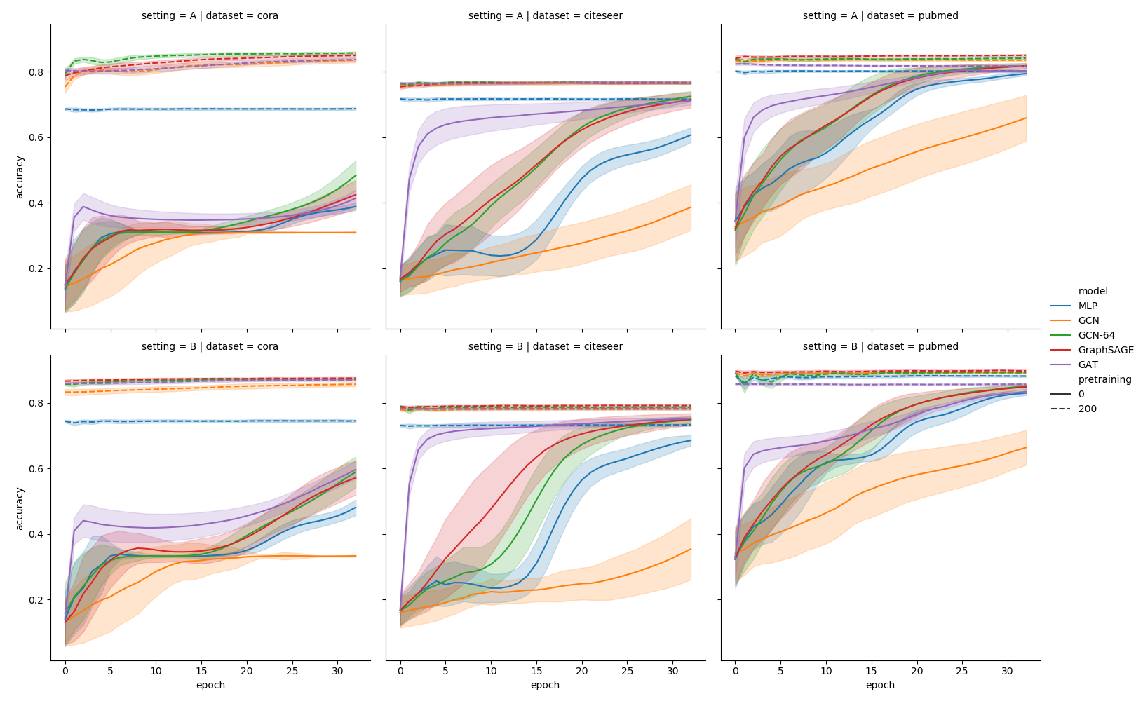
Figure 1: Test accuracy after each inference epoch for the many-few settings A (Top) and few-many setting B (Bottom) on the datasets Cora, Citeseer, and Pubmed. Each line resembles the mean of 100 runs and its region shows the standard deviation. The dashed lines show the results with 200 pretraining. The solid lines are the results without prertraining.

Figure 1 shows the results of the three models on the three datasets: Cora, Citeseer, and Pubmed. Pretrained models score consistently higher than non-pretrained models while having substantially less variance. The accuracy of the pretrained models plateaus after few inference epochs (up to 10 on Cora-A and Pubmed-B). Without any pretraining, GAT shows the fastest learning process. The absolute scores of pretrained graph neural networks are higher than the ones of MLP. From a broad perspective, the scores of pretrained graph neural networks are all on the same level. While GCN falls behind the others on Cora-B, GAT falls behind the others on Pubmed.

The absolute scores of the many-few setting B are higher than the ones of few-many setting A by a constant margin. We globally compare the results of setting A and B by measuring the Jensen-Shannon divergence (Lin, 1991) between the accuracy distributions. The Jenson-Shannon divergence between the two settings is lower with pretraining (between 0.0057 for GAT and 0.0115 for MLP) than it is without pretraining (between 0.0666 for GraphSAGE to 0.1013 for GCN).

5 Discussion

We have developed an experimental setup to evaluate inferencing capabilities of graph neural networks, which we use to conduct inductive experiments on the well-known citation graph datasets: Cora, Citeseer, and Pubmed. Our results show that graph neural networks perform well even though we insert new nodes and edges after training. For the three datasets considered in this study, the accuracy plateaus after very few inference epochs. This observation holds for both train-test split settings: many-few and few-many. We verified that the accuracy distributions are similar in both train-test splits by measuring the Jenson-Shannon divergence. The low variances of the pretrained models indicate that the 100 runs for each of the pretrained models converge to yield similar accuracy scores and that they are robust against the addition of unseen nodes.

The employed models all consist of two layers. Thus, the models only exploit node features in the two-hop neighborhood of each labeled node. Technically, also more distant nodes’ features would be available, especially during inference. Model depth is, however, still an open issue (Kipf & Welling, 2016a) in the graph domain. Deeper models could, in theory, exploit more distant nodes’ features.

Evaluating inferencing capabilities is important because full re-training might not be feasible on large graphs. We have taken a first step to bring current research in graph neural networks closer to practical applications. Our setup is close to real-world applications, where new nodes appear dynamically over time. Our findings show that maintaining one model and continuing the training process when the data changes is a valid approach for dealing with dynamic graphs.

6 Conclusion

Pretrained graph neural networks yield high accuracy with low variance even though new nodes and edges are inserted into the graph. This property is mandatory for applying graph neural networks to large-scale, dynamic graphs as often found in real-world scenarios.

Reproducibility and reusablity

The source code to reproduce our experiments, to impose our experimental setup on other datasets, or to include further models, is available under github.com/lgalke/gnn-pretraining-evaluation.

References

- Aggarwal & Subbian (2014) Charu Aggarwal and Karthik Subbian. Evolutionary network analysis: A survey. ACM Comput. Surv., 47(1):10:1–10:36, May 2014. ISSN 0360-0300. doi: 10.1145/2601412.
- Bruna et al. (2013) Joan Bruna, Wojciech Zaremba, Arthur Szlam, and Yann LeCun. Spectral networks and locally connected networks on graphs. CoRR, abs/1312.6203, 2013.
- Defferrard et al. (2016) Michaël Defferrard, Xavier Bresson, and Pierre Vandergheynst. Convolutional neural networks on graphs with fast localized spectral filtering. In Advances in Neural Information Processing Systems 29: Annual Conference on Neural Information Processing Systems 2016, December 5-10, 2016, Barcelona, Spain, pp. 3837–3845, 2016.
- Duvenaud et al. (2015) David K Duvenaud, Dougal Maclaurin, Jorge Iparraguirre, Rafael Bombarell, Timothy Hirzel, Alan Aspuru-Guzik, and Ryan P Adams. Convolutional networks on graphs for learning molecular fingerprints. In Advances in Neural Information Processing Systems 28, pp. 2224–2232. Curran Associates, Inc., 2015.
- Galke et al. (2018) Lukas Galke, Florian Mai, Iacopo Vagliano, and Ansgar Scherp. Multi-modal adversarial autoencoders for recommendations of citations and subject labels. In Proceedings of the 26th Conference on User Modeling, Adaptation and Personalization, UMAP ’18, pp. 197–205, New York, NY, USA, 2018. ACM. ISBN 978-1-4503-5589-6. doi: 10.1145/3209219.3209236.
- Glorot & Bengio (2010) Xavier Glorot and Yoshua Bengio. Understanding the difficulty of training deep feedforward neural networks. In Proceedings of the Thirteenth International Conference on Artificial Intelligence and Statistics, AISTATS 2010, Chia Laguna Resort, Sardinia, Italy, May 13-15, 2010, volume 9 of JMLR Proceedings, pp. 249–256. JMLR.org, 2010.
- Hamilton et al. (2017) William L. Hamilton, Zhitao Ying, and Jure Leskovec. Inductive representation learning on large graphs. In Advances in Neural Information Processing Systems 30: Annual Conference on Neural Information Processing Systems 2017, 4-9 December 2017, Long Beach, CA, USA, pp. 1025–1035, 2017.
- Henaff et al. (2015) Mikael Henaff, Joan Bruna, and Yann LeCun. Deep convolutional networks on graph-structured data. CoRR, abs/1506.05163, 2015.
- Kingma & Ba (2014) Diederik P. Kingma and Jimmy Ba. Adam: A method for stochastic optimization. CoRR, abs/1412.6980, 2014.
- Kipf & Welling (2016a) Thomas N. Kipf and Max Welling. Semi-supervised classification with graph convolutional networks. CoRR, abs/1609.02907, 2016a. Published at ICLR 2017.
- Kipf & Welling (2016b) Thomas N. Kipf and Max Welling. Variational graph auto-encoders. CoRR, abs/1611.07308, 2016b.
- Li et al. (2015) Yujia Li, Daniel Tarlow, Marc Brockschmidt, and Richard S. Zemel. Gated graph sequence neural networks. CoRR, abs/1511.05493, 2015.
- Lin (1991) Jianhua Lin. Divergence measures based on the shannon entropy. IEEE Trans. Information Theory, 37(1):145–151, 1991. doi: 10.1109/18.61115.
- Sen et al. (2008) Prithviraj Sen, Galileo Namata, Mustafa Bilgic, Lise Getoor, Brian Gallagher, and Tina Eliassi-Rad. Collective classification in network data. AI Magazine, 29(3):93–106, 2008.
- Veličković et al. (2018) Petar Veličković, Guillem Cucurull, Arantxa Casanova, Adriana Romero, Pietro Liò, and Yoshua Bengio. Graph attention networks. International Conference on Learning Representations, 2018.
- Yang et al. (2016) Zhilin Yang, William W. Cohen, and Ruslan Salakhutdinov. Revisiting semi-supervised learning with graph embeddings. In Proceedings of the 33nd International Conference on Machine Learning, ICML 2016, New York City, NY, USA, June 19-24, 2016, volume 48 of JMLR Workshop and Conference Proceedings, pp. 40–48. JMLR.org, 2016.