Measuring Higgs self couplings in the presence of VVH and VVHH at the ILC

Abstract

The recent discovery of a Higgs boson at the LHC, while establishing the Higgs mechanism as the way of electroweak symmetry breaking, started an era of precision measurements involving the Higgs boson. In an effective Lagrangian framework, we consider the $e^{+}e^{-}\rightarrow ZHH$ process at the ILC running at a centre of mass energy of 500 GeV to investigate the effect of the $ZZH$ and $ZZHH$ couplings on the sensitivity of $HHH$ coupling in this process. Our results show that the sensitivity of the trilinear Higgs self couplings on this process has somewhat strong dependence on the Higgs-gauge boson couplings. Single and two parameter reach of the ILC with an integrated luminosity of 1000 fb^-1 are obtained on all the effective couplings indicating how these limits are affected by the presence of anomalous $ZZH$ and $ZZHH$ couplings. The kinematic distributions studied to understand the effect of the anomalous couplings, again, show a strong influence of $Z$-$H$ couplings on the dependence of these distributions on $HHH$ coupling. Similar results are indicated in the case of the process, $e^{+}e^{-}\rightarrow\nu\bar{\nu}HH$, considered at a centre of mass energy of 2 TeV, where the cross section is large enough. The effect of $WWH$ and $WWHH$ couplings on the sensitivity of $HHH$ coupling is clearly established through our analyses in this process.

I Introduction

With the discovery of the new resonance of mass around 125 GeV at the LHC Chatrchyan:2012xdj ; Aad:2012tfa ; ATLAS:2013xla ; ATLAS:2013nma ; ATLAS:2013vla ; CMS:xwa ; CMS:bxa ; Aad:2013wqa ; Chatrchyan:2012xdj ; Chatrchyan:2013lba ; Aad:2012tfa ; ATLAS:2016oum ; ATLAS:2016pkl ; ATLAS:2016zzs ; Aad:2015vsa ; ATLAS:2016hru , a new era is open in the investigations of elementary particle dynamics. The new particle is so far consistent in every way with the long expected Higgs boson of the Standard Model (SM). All the expected SM decays are observed at the LHC, albeit some tension in the decay widths, which are still consistent within the statistical fluctuations. The spin and parity analysis favour a spin-zero, even-parity object ATLAS:2013xla ; ATLAS:2013nma ; ATLAS:2013vla ; CMS:xwa ; CMS:bxa ; Aad:2015mxa . These measurements establish the role of Higgs mechanism in the electroweak symmetry breaking (EWSB) and the discovered resonance as the Higgs boson. So far the measurements are consistent with the properties of the Higgs boson expected in the SM Higgs mechanism. While we wait for further statistics to establish more detailed identity of this discovery, it is worth revisiting the role of new physics in the Higgs sector in the light of the new measurements. It is well accepted that, even if all the properties of the new particle meets the expectations of the SM, there still remain several questions on the SM. One of the serious issues within the Higgs sector is the difficulty with quadratically diverging quantum corrections to the mass of the Higgs boson, or the so called hierarchy problem. This itself should convince us that the SM is at the most effective theory, highly successful at the electroweak scale. Another contentious issue is the stability of the vacuum. With the quantum corrections to the quartic Higgs coupling that the massive fermions and gauge bosons would induce, it is indicated that the minimum of the potential corresponds to a local metastable vacuum, with a possible global vacuum at much higher energies Degrassi:2012ry . Among the plethora of suggestions to look beyond the SM, one could indeed narrow down to scenarios that can accommodate a light Higgs boson, very likely an elementary one, with properties very close to that of the SM Higgs boson. One may need to wait till the LHC reveals further indications of new physics, if we are lucky, or perhaps even need to wait till the new generation lepton colliders, like the International Linear Collider (ILC) BrauJames:2007aa ; Djouadi:2007ik ; MoortgatPick:2005cw , start exploring the TeV scale physics. Being a discovery machine, the LHC is capable of observing any direct production of new particle resonance at the energy scales explored, while the latter is more suitable to explore the new physics through detailed precision analysis, in the absence of any such direct observation of new physics.

Taking a cue from the observations so far, we are compelled to consider a case with new physics somewhat decoupled from the electroweak physics, which in turn is dictated by the SM. In that case, the effect of new physics will be reflected in the various couplings through the quantum corrections they acquire. The best way to study such effects is through an effective Lagrangian, which encodes the new physics effects in higher dimensional operators with anomalous couplings. Interesting phenomenological studied with effective Higgs couplings, including the possibility of CP violation in the Higgs sector is discussed in the literature . The study of Higgs sector through an effective Lagrangian, and effective couplings goes back to Refs.Weinberg:1978kz ; Weinberg:1980wa ; Georgi:1994qn ; Buchmuller:1985jz ; Hagiwara:1993ck ; Hagiwara:1993qt ; Alam:1997nk ; Barger:2003rs ; Giudice:2007fh ; Grzadkowski:2010es ; Contino:2010rs ; Grzadkowski:2010es ; Grzadkowski:2010es ; GutierrezRodriguez:2011gi ; GutierrezRodriguez:2009uz ; GutierrezRodriguez:2005fe ; Rindani:2010pi ; Rindani:2009pb . More recently, the Lagrangian including complete set of dimension-6 operators was studied in Refs. Baak:2012kk ; Einhorn:2013kja ; Contino:2013kra ; Amar:2014fpa ; Masso:2014xra ; Biekoetter:2014jwa ; Willenbrock:2014bja . For some of the recent reference discussing the constraints on the anomalous couplings within different approches, please see Bonnet:2011yx ; Corbett:2012dm ; Chang:2013cia ; Elias-Miro:2013mua ; Banerjee:2013apa ; Boos:2013mqa ; Masso:2012eq ; Han:2004az ; Corbett:2012ja ; Dumont:2013wma ; Pomarol:2013zra ; Ellis:2014dva ; Belusca-Maito:2014dpa ; Gupta:2014rxa ; Ellis:2017kfi ; Denizli:2017pyu ; DiVita:2017vrr ; Ellis:2018gqa ; Liu:2018peg ; Rindani:2018ubx ; Hesari:2018ssq . Ref. Ellis:2014dva studied the H+V, where V= Z, W, associated production at the LHC and the Tevatron to discuss the bounds obtainable from the global fit to the presently available data, whereas Refs. Belusca-Maito:2014dpa and Ellis:2018gqa discuss the constraint on the parameters coming from the LHC results as well as other precision data from LEP, SLC and the Tevatron. Experimental studies on the Higgs couplings at the LHC are presented in, for example, Aad:2013wqa ; Teyssier:2014hta ; ATLAS:2018otd ; Khachatryan:2016vau ; CMS:2013xfa .

Higgs self couplings give direct information about the scalar potential, and therefore, very important to understand the nature of the EWSB. The process, $e^{+}e^{-}\rightarrow ZHH$ is one of the best suited to study the Higgs trilinear coupling DeRujula:1991ufe ; GutierrezRodriguez:2008nk ; Takubo:2009ws ; Tian:2010np ; Battaglia:2001nn ; Barger:2003rs ; Killick:2013mya ; Djouadi:1999gv ; Baer:2013cma ; Castanier:2001sf ; Liu:2018peg . At the same time, this process also depends on the Higgs-Gauge boson couplings, $ZZH$ and $ZZHH$, which will affect the determination of the the $HHH$ coupling. Another process that could probe the $HHH$ couplings is $e^{+}e^{-}\rightarrow\nu\bar{\nu}HH$ following the WW fusion Battaglia:2001nn ; Barger:2003rs ; Killick:2013mya ; Djouadi:1999gv ; Rindani:2018ubx , which is also affected by the $WWH$ and $WWHH$ couplings. With the first phase of the ILC expected to run at 250 GeV centre of mass energy, efforts to probe the $ZH$ production process, where the influence of the quartic couplings would be felt at one loop, are seriously studied Rindani:2018ubx ; DiVita:2017vrr . In this report we will focus on the Higgs pair production processes within the framework of the effective Lagrangian. One goal of this study is to investigate how significant is the effect of $VVH$ coupling, where $V=Z,~{}W$, in the extraction of the $HHH$ coupling. In contrast to other similar studies, we perform a multi-parameter analysis employing the Markov-Chain-Monte-Carlo method to obtain simultaneous constraints in hyperspace spanned by all relevant parameters.

The report is presented in the following way. In Section II the effective Lagrangian will be presented, with the currently available constraint on the parameters. In Section III the processes under consideration will be presented, with details. In Section IV the results will be summarized.

II General Setup

The effective Lagrangian with full set of dimension-6 operator involving the Higgs bosons is described in Ref.  Giudice:2007fh ; Grzadkowski:2010es ; Contino:2010rs ; Grzadkowski:2010es ; Contino:2013kra ; Ellis:2014dva . In this report, we shall restrict our discussion to the processes $e^{+}e^{-}\rightarrow ZHH$, and $e^{+}e^{-}\rightarrow\nu\bar{\nu}WW\rightarrow\nu\bar{\nu}HH$. Relevant to these processes, part of the Lagrangian is given by

$${\cal L}_{\rm Higgs}^{\rm anom} = \frac{\bar{c}_{H}}{2v^{2}}\partial^{\mu}\big{(}\Phi^{\dagger}\Phi\big{)}\partial_{\mu}\big{(}\Phi^{\dagger}\Phi\big{)}+\frac{\bar{c}_{6}}{v^{2}}\lambda~{}\big{(}\Phi^{\dagger}\Phi\big{)}^{3}+\frac{\bar{c}_{\gamma}}{m_{W}^{2}}g^{\prime 2}~{}\Phi^{\dagger}\Phi B_{\mu\nu}B^{\mu\nu}+\frac{\bar{c}_{g}}{m_{W}^{2}}g_{s}^{2}~{}\Phi^{\dagger}\Phi G_{\mu\nu}^{a}G_{a}^{\mu\nu}$$ (1)

$$+\frac{\bar{c}_{HW}}{m_{W}^{2}}ig~{}\big{(}D^{\mu}\Phi^{\dagger}\sigma_{k}D^{\nu}\Phi\big{)}W_{\mu\nu}^{k}+\frac{\bar{c}_{HB}}{m_{W}^{2}}ig^{\prime}~{}\big{(}D^{\mu}\Phi^{\dagger}D^{\nu}\Phi\big{)}B_{\mu\nu}\$$

$$+\frac{\bar{c}_{W}}{2m_{W}^{2}}ig~{}\big{(}\Phi^{\dagger}\sigma_{k}\overleftrightarrow{D}^{\mu}\Phi\big{)}D^{\nu}W_{\mu\nu}^{k}+\frac{\bar{c}_{B}}{2m_{W}^{2}}ig^{\prime}~{}\big{(}\Phi^{\dagger}\overleftrightarrow{D}^{\mu}\Phi\big{)}\partial^{\nu}B_{\mu\nu},$$

where $\Phi^{\dagger}{\overleftrightarrow{D}}_{\mu}\Phi=\Phi^{\dagger}D^{\mu}\Phi-D_{\mu}\Phi^{\dagger}\Phi\ ,$ $D^{\mu}$ being the appropriate covariant derivative operator, and $\Phi$, the usual Higgs doublet in the SM. Also, $G_{\mu\nu}^{a}$, $W_{\mu\nu}^{k}$ and $B_{\mu\nu}$ are the field tensors corresponding to the $SU(3)_{C}$, $SU(2)_{L}$ and $U(1)_{Y}$ of the SM gauge groups, respectively, with gauge couplings $g_{s}$, $g$ and $g^{\prime}$, in that order. $\sigma_{k}$ are the Pauli matrices, and $\lambda$ is the usual (SM) quadratic coupling constant of the Higgs field. The above Lagrangian leads to the following in the unitary gauge and mass basis  Alloul:2013naa

$${\cal L}_{H,Z,W}^{\rm anom}= -v\lambda g_{HHH}^{(1)}H^{3}+\frac{1}{2}g_{HHH}^{(2)}H\partial_{\mu}H\partial^{\mu}H-\frac{1}{4}g_{HZZ}^{(1)}Z_{\mu\nu}Z^{\mu\nu}H-\frac{1}{4}g_{HZZ}^{(2)}Z_{\nu}\partial_{\mu}Z^{\mu\nu}H$$

$$+\frac{1}{2}g_{HZZ}^{(3)}Z_{\mu}Z^{\mu}H-\frac{1}{2}g_{HAZ}^{(1)}Z_{\mu\nu}F^{\mu\nu}H-g_{HAZ}^{(2)}Z_{\nu}\partial_{\mu}F^{\mu\nu}H$$

$$-\frac{1}{8}g_{HHZZ}^{(1)}Z_{\mu\nu}Z^{\mu\nu}H^{2}-\frac{1}{2}g_{HHZZ}^{(2)}Z_{\nu}\partial_{\mu}Z^{\mu\nu}H^{2}-\frac{1}{4}g_{HHZZ}^{(3)}Z_{\mu}Z^{\mu}H^{2}$$

$$-\frac{1}{2}g_{HWW}^{(1)}W^{\mu\nu}W_{\mu\nu}^{\dagger}H-\left[g_{HWW}^{(2)}W^{\nu}\partial^{\mu}W_{\mu\nu}^{\dagger}H+h.c.\right]+g~{}m_{W}W_{\mu}^{\dagger}W^{\mu}H$$

$$-\frac{1}{4}g_{HHWW}^{(1)}W^{\mu\nu}W_{\mu\nu}^{\dagger}H^{2}-\frac{1}{2}\left[g_{HHWW}^{(2)}W^{\nu}\partial^{\mu}W_{\mu\nu}^{\dagger}H^{2}+h.c.\right]+\frac{1}{4}g^{2}W_{\mu}^{\dagger}W^{\mu}H^{2}$$

Various physical couplings present in the Lagrangian in Eq. (LABEL:eq:LagPhys) are given in terms of the parameters of the effective Lagrangian in Eq. (1) as

$$g_{HHH}^{(1)}=1+\frac{5}{2}\bar{c_{6}},\hskip 28.45274ptg_{HHH}^{(2)}=\frac{g}{m_{W}}\bar{c}_{H}$$

$$g_{HZZ}^{(1)}=\frac{2g}{c_{W}^{2}m_{W}}\left[\bar{c}_{HB}s_{W}^{2}-4\bar{c}_{\gamma}s_{W}^{4}+c_{W}^{2}\bar{c}_{HW}\right]$$

$$g_{HZZ}^{(2)}=\frac{g}{c_{W}^{2}m_{W}}\left[(\bar{c}_{HW}+\bar{c}_{W})c_{W}^{2}+(\bar{c}_{B}+\bar{c}_{HB})s_{W}^{2}\right],~{}~{}~{}~{}~{}g_{HZZ}^{(3)}=\frac{gm_{Z}}{c_{W}}\left[1-2\bar{c}_{T}\right]$$

$$g_{HAZ}^{(1)}=\frac{gs_{W}}{c_{W}m_{W}}\left[\bar{c}_{HW}-\bar{c}_{HB}+8\bar{c}_{\gamma}s_{W}^{2}\right]$$

$$g_{HAZ}^{(2)}=\frac{gs_{W}}{c_{W}m_{W}}\left[\bar{c}_{HW}-\bar{c}_{HB}-\bar{c}_{B}+\bar{c}_{W}\right]$$

$$g_{HHZZ}^{(1)}=\frac{g^{2}}{c_{W}^{2}m_{W}^{2}}\left[\bar{c}_{HB}s_{W}^{2}-4\bar{c}_{\gamma}s_{W}^{4}+\bar{c}_{HW}c_{W}^{2}\right]$$

$$g_{HHZZ}^{(2)}=\frac{g^{2}}{2c_{W}^{2}m_{W}^{2}}\left[(\bar{c}_{HW}+\bar{c}_{W})c_{W}^{2}+(\bar{c}_{B}+\bar{c}_{HB})s_{W}^{2}\right],~{}~{}~{}~{}~{}g_{HHZZ}^{(3)}=\frac{g^{2}}{2c_{W}^{2}}\left[1-6\bar{c}_{T}\right]$$

$$g_{HWW}^{(1)}=\frac{2g}{m_{W}}\bar{c}_{HW},~{}~{}~{}~{}~{}~{}~{}~{}g_{HWW}^{(2)}=\frac{g}{2m_{W}}\left[\bar{c}_{W}+\bar{c}_{HW}\right]$$

$$g_{HHWW}^{(1)}=\frac{g^{2}}{m_{W}^{2}}\bar{c}_{HW},~{}~{}~{}~{}~{}~{}g_{HHWW}^{(2)}=\frac{g^{2}}{4m_{W}^{2}}\left[\bar{c}_{W}+\bar{c}_{HW}\right]$$ (3)

In total eight coefficients, namely, $\bar{c}_{6},~{}\bar{c}_{H},~{}\bar{c}_{T},~{}\bar{c}_{\gamma},~{}\bar{c}_{B},~{}\bar{c}_{W},~{}\bar{c}_{HB},~{}\bar{c}_{HW}$, govern the dyanmics of $ZHH$ and $\nu\bar{\nu}HH$ productions at the ILC. Coming to the experimental constraints on these parameters, the first two, $\bar{c}_{6}$ and $\bar{c}_{H}$ influence only the Higgs self couplings, and therefore, practically, do not have any experimental constraints on them. Electroweak precision tests constrain $\bar{c}_{T}$, $\bar{c}_{W}$ and $\bar{c}_{B}$ as  Baak:2012kk

$$\bar{c}_{T}(m_{Z})\in[-1.5,2.2]\times 10^{-3},$$

$$(\bar{c}_{W}(m_{Z})+\bar{c}_{B}(m_{Z}))\in[-1.4,1.9]\times 10^{-3}.$$ (4)

Note that, $\bar{c}_{W}$ and $\bar{c}_{B}$ are not independently constrained, leaving a possibility of having large values with a cancellation between them as per the above constraint. $\bar{c}_{W}$ itself, along with $\bar{c}_{HW}$ and $\bar{c}_{HB}$ is constrained from the LHC observations on the associated production of Higgs along with $W$ in Ref.  Ellis:2014dva . Consideration of the Higgs associated production along with W, ATLAS and CMS along with D0 put a limit of $\bar{c}_{W}\in\big{[}-0.05,0.04\big{]}$, when all other parameters are set to zero. A global fit using various information from ATLAS and CMS, including signal-strength information constrains the region in $\bar{c}_{W}-\bar{c}_{HW}$ plane, leading to a slightly more relaxed limit on $\bar{c}_{W}$, and a limit of about $\bar{c}_{HW}\in\big{[}-0.1,0.06\big{]}$. The limit on $\bar{c}_{HB}$ estimated using a global fit in Ref. Ellis:2014dva is about $\bar{c}_{HB}\in[-0.05,0.05]$ with a one parameter fit.

The purpose of this study is to understand how to exploit a precision machine like the ILC to investigate suitable processes so as to derive information regarding these couplings. In the next section we shall explain the processes of interest in the present case, and discuss the details to understand the influence of one or more of the couplings mentioned above.

III Discussion of the processes considered

It is generally expected that the ILC, with its clean environment, fixed centre of mass energy, and additional features like availability of beam polarization, will be able to do the precision studies much more efficiently than what the LHC could do. This is especially so in the case of Higgs self couplings. One of the best suited process to study the trilinear (self) coupling of the Higgs boson is $e^{+}e^{-}\rightarrow ZHH$, the phenomenological analysis of which is studied in detail within the context of the SM. The Feynman diagrams corresponding to this process in the SM are given in Fig. 1.

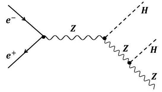
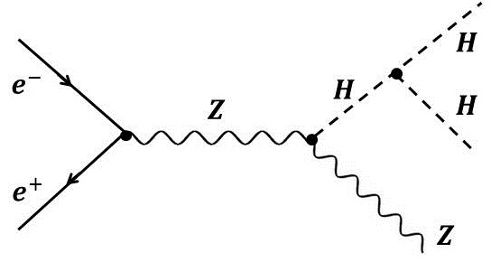
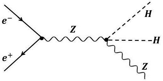
Figure 1: Feynman diagrams contributing to the process $e^{-}e^{+}\rightarrow ZHH$ in Standard Model.

Another process that is relevant to the study of $HHH$ coupling is $e^{+}e^{-}\rightarrow\nu_{e}\bar{\nu}_{e}HH$. The earlier process, $e^{+}e^{-}\rightarrow ZHH$, with the invisible decay of $Z\rightarrow\nu_{e}\bar{\nu}_{e}$ also leads to the same final state. However, this can be easily reduced by considering the missing invariant mass. The rest of the process goes through the Feynman diagrams presented in Fig. 2.

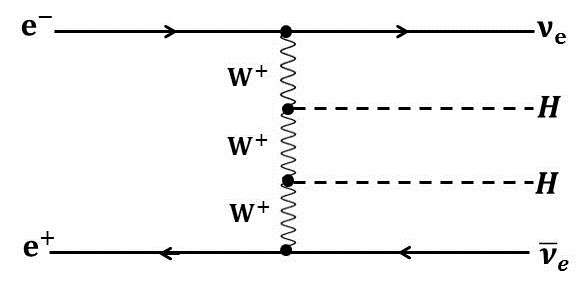
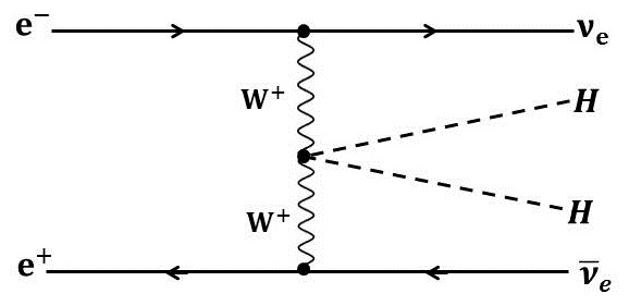
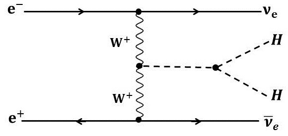
Figure 2: Feynman diagrams contributing to the process $e^{-}e^{+}\rightarrow\nu\bar{\nu}HH$ in Standard Model, without considering $e^{+}e^{-}\rightarrow ZHH\rightarrow\nu\bar{\nu}HH$

Apart from the $HHH$ coupling, these processes are influenced by gauge-Higgs couplings like $ZZH$, $ZZHH$, $WWH$ and $WWHH$. Keeping in mind the above discussion of the effective couplings deviating from the SM due to the influence of the BSM at some higher energies, one must understand how such a scenario would affect the phenomenology, in order to draw any conclusion regarding these couplings. In the rest of this report, we shall revisit these processes, with a specific purpose of understanding the correlation between the gauge-Higgs coupling and the trilinear Higgs couplings.

For our analyses we use MadGraph5 Alwall:2014hca , with the Effective Lagrangian implemented through FeynRules Alloul:2013bka as given by Alloul:2013naa .

III.1 $e^{+}e^{-}\rightarrow ZHH$ Process

We shall first consider $e^{+}e^{-}\rightarrow ZHH$ process. In Fig. 3 the cross section is plotted against the centre of mass for the SM case as well as for some selected $(c_{6},c_{H})$ points. The cross section peaks around a centre of mass energy of 600 GeV with a value of about 0.17 fb, which slides down to about 0.16 fb at 500 GeV. We perform our analysis for the ILC running at a centre of mass energy of 500 GeV.

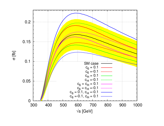
Figure 3: Cross section against $\sqrt{s}$ for the process $e^{-}e^{+}\rightarrow ZHH$, for different values of the parameters $c_{6}$ and $c_{H}$, with all others kept to zero.

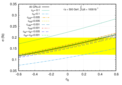
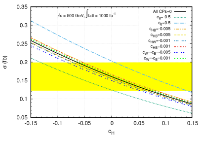
Figure 4: Cross section of $ZHH$ production against $c_{6}$ (left) and $c_{H}$ (right), when some of the other selected relevant parameters assume typical values is compared against the case when only $c_{6}$ or $c_{H}$ is present. The black solid lines corresponds to the case when all parameters other than $c_{6}$ (left) or $c_{H}$ (right) vanish. The centre of mass energy is assumed to be $\sqrt{s}=500$ GeV. In each case, all other parameters are set to zero. The yellow band indicates the $3\sigma$ limit of the SM cross section, with integrated luminosity of $1000$ fb^-1.

To seek a functional form of cross section as a function of the anomalous couplings we generated events in MadGraph5 for the process $e^{+}e^{-}\to hhZ$ with and without decaying the particles with $100$ random set of couplings $f_{i}=(c_{6},c_{H},c_{W},c_{B},c_{HB},c_{HW})$ within a given range at $\sqrt{s}=500$ GeV and fitted the cross section of the process with the formula

$$\sigma=\sigma_{0}+f_{i}\times\sigma_{i}+f_{i}\times f_{j}\times\sigma_{ij}.$$ (5)

Here $\sigma_{0}$ is the cross section when $f_{i}=0$, i.e., the SM cross section. The production cross section of $e^{+}e^{-}\to hhZ$ at $\sqrt{s}=500$ GeV as a function of the anomalous higgs couplings ($c_{6},c_{H},c_{W},c_{B},c_{HB},c_{HW}$) is obtained to be

$$\sigma = 0.160868+0.0787057\times c_{6}-0.571945\times c_{H}+2.64522\times c_{W}-0.0588928\times c_{B}$$ (6)

$$+ 1.09184\times c_{HB}+5.69175\times c_{HW}+0.0119329\times c_{6}^{2}+0.523069\times c_{H}^{2}+121.355\times c_{W}^{2}$$

$$- 0.0636082\times c_{B}^{2}+57.9799\times c_{HB}^{2}+110.68\times c_{HW}^{2}-0.150628\times c_{6}\times c_{H}$$

$$+ 0.683334\times c_{6}\times c_{W}-0.000703205\times c_{6}\times c_{B}+0.266043\times c_{6}\times c_{HB}+1.39575\times c_{6}\times c_{HW}$$

$$- 4.89070\times c_{H}\times c_{W}-0.00250087\times c_{H}\times c_{B}-1.9789\times c_{H}\times c_{HB}-10.1718\times c_{H}\times c_{HW}$$

$$+ 0.00489508\times c_{W}\times c_{B}+165.005\times c_{W}\times c_{HB}-107.031c_{W}\times c_{HW}$$

$$+ 0.0343358\times c_{B}\times c_{HB}+0.0649916\times c_{B}\times c_{HW}-89.6786\times c_{HB}\times c_{HW}~{}~{}~{}\text{fb}.$$

The total cross section including the decay of $Z\to l^{+}l^{-}$ and $h\to b\bar{b}$ would be

$$\sigma_{tot}=\sigma\times Br(Z\to l^{+}l^{-})\times Br(h\to b\bar{b})^{2}~{}~{}~{}\text{fb}.$$ (7)

The influence of $c_{6}$ and $c_{H}$ on the production cross section given in Eq. (6) are shown in Fig. 4 in the left-panel and in the right-panel, respectively. We compare the variation of cross section with $c_{6}$ keeping all other parameters to the SM value, with the cases when some of the relevant parameters having non-standard values. The $3\sigma$ region (yellow band) of the SM value of the cross section, considering an integrated luminosity of 1000 fb^-1, is presented in these plots so as to make an estimate of the reach on the $c_{6}$. The plots clearly indicate the correlation between the influence of different parameters on the cross section. For example, assuming only $c_{6}$ takes a non-zero value, the reach at $3\sigma$ level is approximately $-0.5<c_{6}<0.45$, as indicated by the black solid line. However, as indicated by the red solid line, if we assume a typical value of $c_{W}=-c_{B}=-0.005$, the lower limit is considerably relaxed, with some moderate change in the upper bound to 0.5. On the other hand, for the case with $c_{W}=-c_{B}=0.001$, where the sign is reversed, the upper bound becomes more stringent, whereas the lower bound is more relaxed. A similar story can be read out for the cases with the presence of other parameters as well. The effect of all the parameters $c_{W}$, $c_{HW}$ and $c_{HB}$, which contribute to the $ZZH$ and $ZZHH$ couplings are found to be significant. Strong dependence of the sensitivity of $c_{6}$ on the presence of $c_{H}$ is somewhat expected, for both parameters contribute to the $HHH$ coupling. The dependence on all the parameters on the sensitivity of $c_{H}$ on the cross section is also found to be significant for chosen typical values of the parameters.

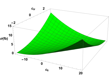
Figure 5: Cross section of $ZHH$ production plotted against $c_{6}$ and $c_{H}$ at $\sqrt{s}=500$ GeV, with all other parameters set to zero.

To see the simultaneous effect of $c_{6}$ and $c_{H}$, the production cross section given in is plotted against $c_{6}$ and $c_{H}$ In Fig. 5. The correlation of the sensitivity between the two parameters is clear. The opposite sign combination seems to be more sensitive to the cross section, and therefore more stringent constraints could be drawn in this case compared to the same sign case.

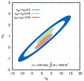
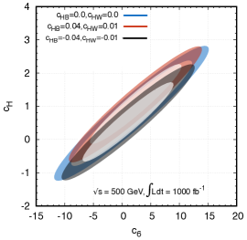
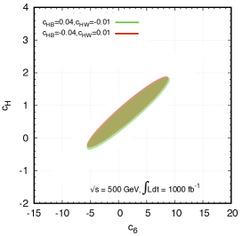
Figure 6: The shaded regions correspond to regions in the $c_{6}$-$c_{H}$ plane with the total cross section is within the $3\sigma$ limit when $c_{6}=c_{H}=0$ in each case, for an integrated luminosity of $1000$ fb^-1 at a centre of mass energy of $500$ GeV. Values of the other anomalous couplings are as indicated in the figure, with all other couplings set to zero.

The reach of the ILC on the trilinear Higgs coupling through the process being considered can be established by considering the $3\sigma$ limit of the cross section at an integrated luminosity of 1000 $fb^{-1}$ as presented in Fig. 6, for the case of SM, and cases with non-vanishing anomalous $ZZH$ and $ZZHH$ couplings. Please note that, when cross section is considered as a function of $c_{6}$ and $c_{H}$, the result is a second order polynomial with these two parameters (see Eq. (6)). With this, the $3\sigma$ limit of the cross section leads to an elliptic equation corresponding to the relation between these two parameters. This result in an elliptic band in the $c_{6}-c_{H}$ plane respecting the $3\sigma$ limit of the cross section. As is evident from the plots, these allowed bands of the parameters move in the parameter space, depending on the values of the other parameters, as illustrated by the cases of $c_{W}=-c_{B}$, $c_{HW}$ and $c_{HB}$. These results also illustrate how important the signs of different couplings are in a study of the sensitivity of the trilinear Higgs couplings. What we may learn from the above is that the limits drawn with assuming the absence of all other parameters may not depict the actual situation.

It is important to know the behaviour of the kinematic distributions, and how the anomalous parameters influence these, to derive any useful and reliable conclusions from the experimental results. This is so, even in cases where the fitting to obtain the reach of the parameters is done with the total number of events, as the reconstruction of events and the reduction of the background depend crucially on the kinematic distributions of the decay products. In the following, we shall present some illustrative cases of distributions at the production level, in order to understand the effect of different couplings on these. The changes in the kinematic distributions at the production level will also be carried over to the distributions of their decay products. Presently we would like to be content with the analysis at the production level, considering the limited scope of this work. As mentioned earlier we shall focus on the ILC running at a centre of mass energy of 500 GeV for our study.

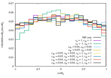
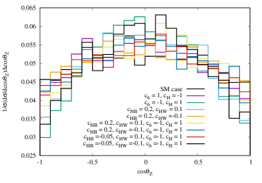
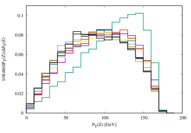
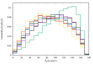
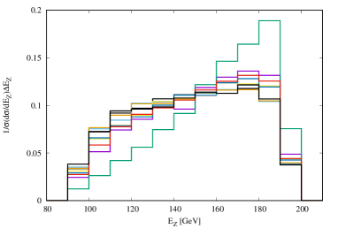
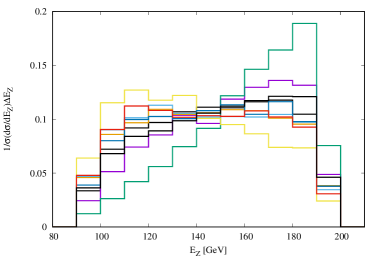
Figure 7: Distributions of the $\cos\theta_{Z}$, Transverse Momentum, and Energy of the $Z$ boson for the anomalous coupling values as in the inset, illustrating how the presence of $c_{W}$ (first column), and $c_{HW}$ and $c_{HB}$ (second column) affect the influence of $c_{6}$ and $c_{H}$. A centre of mass energy of $500$ GeV is assumed.

We first consider in Fig.7 (top row), the normalized $\cos\theta_{Z}$ distributions of the $Z$ boson for the case of SM, as well as for different cases with anomalous couplings. The normalized distributions present the difference in the shape, which brings out the qualitative difference in a more visible manner. The figure on the left shows the case with $c_{W}=-c_{B}$ taking typical values, while the other parameters set to zero, whereas the figure on the right considers $c_{HW}$ and $c_{HB}$ non-zero, while setting other parameters to zero. The case with only $c_{6}$ and $c_{H}$ taking non-zero values, when compared with the SM case shows a perceivable change in the distribution with more number of events piling in the small $\cos\theta_{Z}$ region. Such experimental observations could, therefore, be considered as an indication of the anomalous $HHH$ coupling. On the other hand, the presence of anomalous $c_{W}$ and $c_{B}$ couplings does not affect the distribution much. More importantly, in their presence, the non-zero $c_{W}$ and $c_{B}$, the distribution remains close to the SM distribution, even with non-zero $c_{6}$ and $c_{H}$. Thus, a conclusion regarding the presence or otherwise of the $HHH$ coupling drawn from the $\cos\theta_{Z}$ distribution will depend on the values of $c_{W}$ and $c_{B}$. The figure on the right tells a similar story for the case of $c_{HW}$ and $c_{HB}$ replacing $c_{W}$. In Fig.7 (second row) and (third row), the $p_{T}$ and energy distributions of the $Z$ boson are plotted. Here too, we see that if only $c_{6}$ and $c_{H}$ are considered to be non-zero, events with high $p_{T}$ and high energy $Z$ bosons are preferred much more in comparison with the SM case. This conclusion is upset with the simultaneous presence of other parameters related to $ZZH$ coupling.

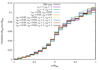
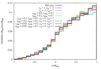
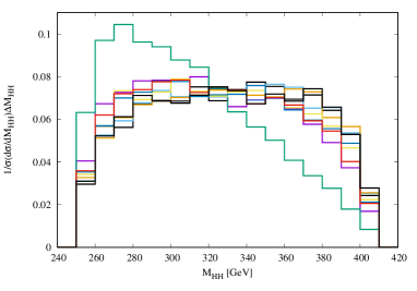
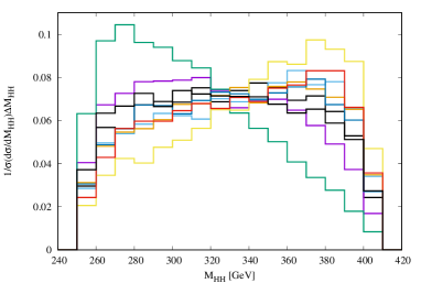
Figure 8: $\cos\theta_{HH}$ and the invariant mass of $HH$ distributions for the anomalous coupling values as in the inset, illustrating how the presence of $c_{W}$ (first column), and $c_{HW}$ and $c_{HB}$ (second column) affect the influence of $c_{6}$ and $c_{H}$. A centre of mass energy of $500$ GeV is assumed.

The distribution of the opening angle between the two Higgs bosons as well as their invariant mass distribution presented in Fig. 8 indicate the same feature captured in the various distributions of the $Z$ bosons. While in all cases including the SM case, most of the events are in the forward hemisphere, in the presence of non-vanishing $c_{6}$ and $c_{H}$, but with $c_{W}=c_{HW}=c_{HB}=0$, the events are more evenly distributed within the forward hemisphere, compared to the rest of the cases including the SM case. The $HH$ invariant mass demonstrate an even more dramatic difference in the different cases mentioned above.

The conclusions that we draw from the above considerations is that single parameter considerations to understand the effect of $HHH$ coupling will not be realistic if other relevant gauge-Higgs couplings receive anomalous contributions. Our preliminary investigation clearly indicates that the correlations can be rather strong, for all the relevant parameters, and one needs to consider a careful analysis to obtain realistic limits on the parameters.

The reach on the parameter $c_{6}$ and $c_{H}$ discussed above uses the production cross section, while the inclusion of decay will loosen the limit on them. Here we use the total cross section including the decay of the $Z$ bosons and the $H$ given in Eq. (7) and study the sensitivity to all the couplings. The sensitivity of the total cross section $\sigma_{tot}$ to a couplings $f$ is defined as

$${\cal S}(f)=\frac{\sigma_{tot}(f)-\sigma_{tot}(f=0)}{\delta\sigma_{tot}},$$ (8)

$\delta\sigma_{tot}$ is the estimated error in $\sigma_{tot}$.

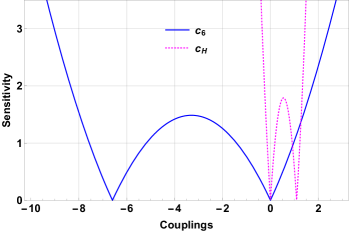
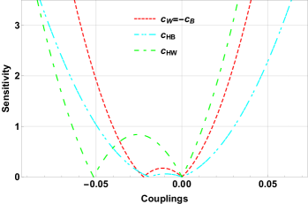
Figure 9: Sensitivity of cross-section on anomalous couplings in $e^{+}e^{-}\to hhZ$ with $h\rightarrow b\bar{b},~{}Z\to l^{+}l^{-}$ for $\sqrt{s}=500$ GeV, ${\cal L}=1000$ fb^-1 for $c_{6}$, $c_{H}$ (left) and $c_{W}=-c_{B}$, $c_{HB}$, $c_{HW}$ (right). The numerical value of one parameter limits on the couplings at $3\sigma$ sensitivity can be read in TABLE 1.

Table 1: Simultaneous limits on anomalous couplings from MCMC in $e^{+}e^{-}\to hhZ$ with $h\rightarrow b\bar{b},~{}Z\to l^{+}l^{-}$ for $\sqrt{s}=500$ GeV, ${\cal L}=1000$ fb^-1

Parameter	68 % BCI	95 % BCI	99 % BCI	One param. $3\sigma$ limit
$c_{6}$	$\in[-5.4,+10]$	$\in[-12,+15]$	$\in[-15,+18]$	$\in[-9.2,+2.4]$
$c_{H}$	$\in[-1.3,+3.1]$	$\in[-3.1,+4.6]$	$\in[-4.1,+5.6]$	$\in[-0.34,+1.4]$
$c_{W}=-c_{B}$	$\in[-0.19,+0.17]$	$\in[-0.34,+0.32]$	$\in[-0.43,+0.41]$	$\in[-0.05,+0.03]$
$c_{HB}$	$\in[-0.21,+0.23]$	$\in[-0.39,+0.41]$	$\in[-0.48,+0.51]$	$\in[-0.07,+0.05]$
$c_{HW}$	$\in[-0.10,+0.10]$	$\in[-0.18,+0.17]$	$\in[-0.23,+0.22]$	$\in[-0.08,+0.02]$

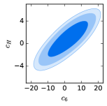
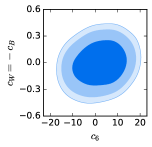
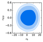
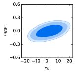
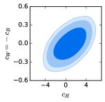
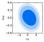
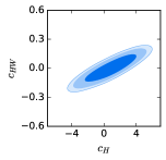
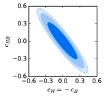
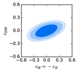
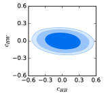
Figure 10: The MCMC $68~{}\%$ (darkest-shaded), $95~{}\%$ (less darker-shaded), $99~{}\%$ (lighter-shaded) BC contours on the parameter space in $e^{+}e^{-}\to hhZ$ with $h\rightarrow b\bar{b},~{}Z\to l^{+}l^{-}$ for $\sqrt{s}=500$ GeV, ${\cal L}=1000$ fb^-1

In Fig.9, we present the sensitivity of the total cross section given in Eq. (7) to all the couplings at center of mass energy of $500$ GeV and Integrated luminosity of $1000$ $fb^{-1}$. Due to the presence of linear piece along with quadratic piece, the sensitivity of $c_{6}$ and $c_{H}$ in the left-panel has double hump nature. Both $c_{6}$ and $c_{H}$ has roughly symmetric limits at $1\sigma$ ($c_{6}\in[-1.4,1.0]$) but these get asymmetric limits at $3\sigma$ ($c_{6}\in[-9.20,+2.43]$) due to the double hump nature. The couplings $c_{W}=-c_{B}$, $c_{HB}$ and $c_{HW}$ shown in the right-panel posses asymmetric limit at $1\sigma$ as well as at $3\sigma$ sensitivity. The one parameter limit at $3\sigma$ sensitivity on all the couplings are shown in the last column of TABLE 1.

We perform a simultaneous multi-parameter analysis with the total cross section using the Markov-Chain–Monte-Carlo (MCMC) method. We obtain simultaneous limits by varying all the couplings simultaneously using GetDist Antony:GetDist package with the MCMC chain. The $68~{}\%$, $95~{}\%$ and $99~{}\%$ Bayesian-Confidence-Interval (BCI) on the couplings are shown in the TABLE 1. The $99~{}\%$ BCI on the couplings can be compared with the $3\sigma$ one parameter limit from sensitivity on the fifth column of the same table. It can be seen that the simultaneous limits on $c_{6}$ are much tighter than its one parameter limit by its parametric dependence, while simultaneous limits on all other couplings are less tighter than their one parameter limit. The correlation among all parameter after marginalization in the remaining parameters are studied and they are shown in Fig. 10. In the figure, the darkest-shaded contours are for $68~{}\%$ BC, less darker-shaded contours are for $95~{}\%$ BC and lightest-shaded contours are for $99~{}\%$ BC. The (anti) correlations among the couplings have emerged in the multi-parameter analysis. A mild correlation can be seen in the panel $c_{6}$–$c_{H}$ and $c_{W}$–$c_{HW}$, while a strong anti-correlation is observed in the panel $c_{W}=-c_{B}$–$c_{HB}$.

III.2 $e^{+}e^{-}\rightarrow HH\nu\bar{\nu}$ process

We shall now turn our attention to the second process involving $HHH$ couplings, as well as gauge-Higgs couplings. We consider the two Higgs production with missing energy through the process $e^{+}e^{-}\rightarrow HH\nu\bar{\nu}$. The previous process, $e^{+}e^{-}\rightarrow HHZ$, with $Z\rightarrow\nu\bar{\nu}$ has the same final state. But, this can be easily separated from the rest of the contributions in the SM, to the channels presented in the Feynman diagrams given in Fig. 2, through, for example considering the missing invariant mass. The cross section for the process is plotted against the centre of mass energy for the case of polarized as well as unpolarized beams in Fig. 11. The advantage of very high energy collider is evident here. We shall consider a centre of mass energy of 2 TeV, for which the cross section is close to 0.4 fb in case of unpolarized beams, and slightly more than 1 fb for $e^{-}$ beam of $-80~{}\%$ polarization and $e^{+}$ beam with $+60~{}\%$ polarization Behnke:2013xla . This study will complement the study of the $ZHH$ production in the sense that the physical couplings involved are $HHH$ along with $WWH$ and $WWHH$ instead of the ones involving the neutral gauge bosons. Although in the language of the effective Lagrangian, the couplings involved are similar to the ones in the previous process, their involvement in the current process is expected to be different.

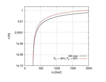
Figure 11: Total cross section of $e^{-}e^{+}\rightarrow\nu_{e}\bar{\nu}_{e}HH$ in the case of unpolarized and polarized beams, as indicated.

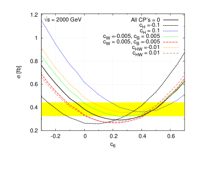
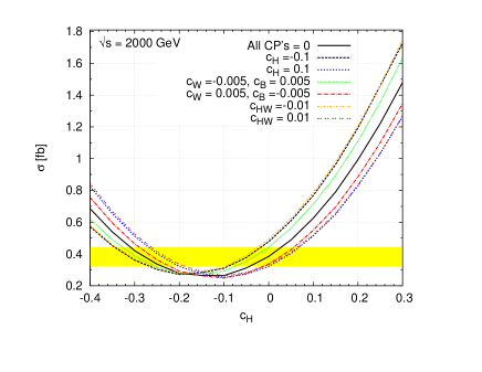
Figure 12: Cross section of $\nu\bar{\nu}HH$ production against $c_{6}$ (left) and $c_{H}$ (right), when some of the other selected relevant parameters assume typical values is compared against the case when only $c_{6}$ or $c_{H}$ is present. The black solid lines corresponds to the case when all parameters other than $c_{6}$ (left) or $c_{H}$ (right) vanish. The centre of mass energy is assumed to be $\sqrt{s}=2$ TeV. In each case, all other parameters are set to zero. The yellow band indicates the $3\sigma$ limit of the SM cross section.

As in the earlier case, the sensitivity of $c_{6}$ and $c_{H}$ on the total cross section at the centre of mass energy of 2 TeV is presented in Figs. 12, where all other parameters are set to zero, as well as in the presence of some of the relevant parameters. We have included the $3\sigma$ band of the SM cross section assuming 1000 fb^-1 luminosity. Clearly, the correlation is perceivable, and the conclusions are similar to the case of $ZHH$ production, that the sensitivity of $HHH$ coupling on the process considered strongly depend on the values of other parameters relevant to $WWH$ and $WWHH$ couplings.

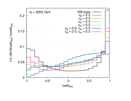
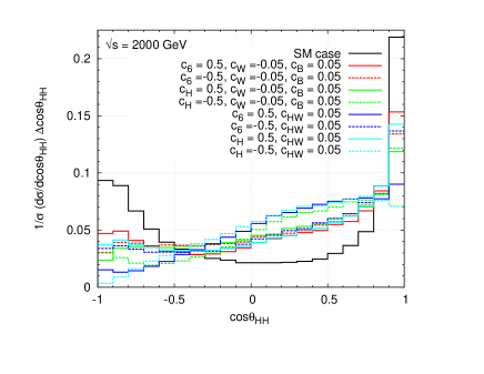
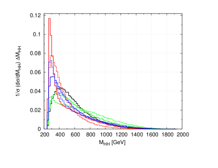
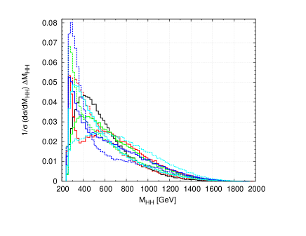
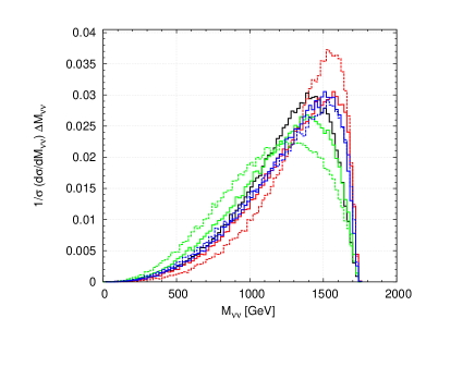
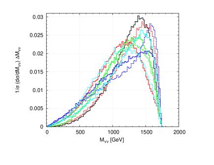
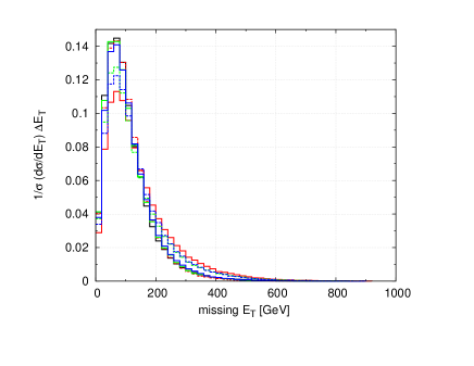
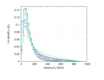
Figure 13: Kinematic distributions with the anomalous coupling values as in the inset, illustrating how the presence of $c_{W}$ (first column), and $c_{HW}$ and $c_{HB}$ (second column) affect the influence of $c_{6}$ and $c_{H}$. A centre of mass energy of $2000$ GeV is assumed.

Moving on to the kinematic distributions, we shall present the distributions of the opening angle between the two Higgs bosons is presented in Fig.13 (first row). The effect of $c_{W}$, and $c_{HW}$ and $c_{HB}$ are presented separately in the first column and the second column, respectively. In both cases, the case with only $c_{6}$ and $c_{H}$ considered to be non-vanishing, and the SM case are presented for comparison. The dependence of the gauge-Higgs coupling on the sensitivity of $HHH$ coupling is clear from the plots. The $HH$ invariant mass, as well as the missing invariant mass distributions, also indicate a similar dependence, as presented in Fig.13 (second row) and (third row). On the other hand, the missing transverse energy distribution does not show much influence of the Higgs-gauge couplings on the sensitivity of $c_{6}$ and $c_{H}$.

IV Summary and Conclusions

The recent discovery of the Higgs boson at the LHC has established the Higgs mechanism as the way to have electroweak symmetry breaking, thus generating masses to all the particles. While the mass of the particle is more or less precisely measured, details like the strengths of its self interactions, its couplings with other particles like the gauge bosons, etc. need to be known precisely to understand and pinpoint the exact mechanism of electroweak symmetry breaking. Precise knowledge of the trilinear Higgs self-coupling, which is typically probed directly through processes involving two Higgs production, play a vital role in reconstructing the Higgs potential. Typically, such processes also involve other couplings from the Higgs sector, like the Higgs-gauge boson couplings. We consider the $ZHH$ and $\nu\bar{\nu}HH$ productions at the ILC to understand the influence of the $ZZH$ and $ZZHH$ couplings, in the first process, and $WWH$ and $WWHH$ couplings, on the second process, on the sensitivity of $HHH$ coupling on this process. Single and two parameter limits on the $c_{6}$ and $c_{H}$ couplings, which are related to the $HHH$ couplings, are considered in the case of the ILC with $\sqrt{s}=500$ GeV and integrated luminosity of 1000 fb^-1, to see how the other parameters, $c_{W}$, $c_{HW}$ and $c_{HB}$ influence the limits. It is seen that these latter parameters have significant influence of the reach of $c_{6}$ and $c_{H}$, indicating that prior, and somewhat precise knowledge of the Higgs-gauge coupling is necessary to draw any conclusion on the influence of trilinear couplings on the process considered. The kinematic distributions also indicate a strong influence of Higgs-gauge couplings, showing that, in the presence of very moderate Higgs-gauge couplings, it is difficult to extract reliable information regarding $c_{6}$ and $c_{H}$. A similar story is unfolded by considerations of $e^{+}e^{-}\rightarrow\nu\bar{\nu}HH$, where the influence of $WWH$ and $WWHH$ on the sensitivity of the trilinear Higgs self-coupling is explored. Concluding, one may need to rely on knowledge of the Higgs gauge couplings from elsewhere, or consider clever observables eliminating or subduing their effects, in order to extract meaningful information regarding the trilinear Higgs couplings.

Acknowledgements S. K. would like to acknowledge the financial support from the SERB-DST, India, under the National Post-doctoral Fellowship programme, Grant No. PDF/2015/000167. R. R. thanks Department of Science and Technology, Government of India for support through DST-INSPIRE Fellowship for doctoral program, INSPIRE CODE IF140075.

References

- (1) CMS Collaboration, S. Chatrchyan et al., Observation of a new boson at a mass of 125 GeV with the CMS experiment at the LHC, Phys. Lett. B716 (2012) 30–61 CMS-HIG-12-028, CERN-PH-EP-2012-220, arXiv:1207.7235 [hep-ex].
- (2) ATLAS Collaboration, G. Aad et al., Observation of a new particle in the search for the Standard Model Higgs boson with the ATLAS detector at the LHC, Phys. Lett. B716 (2012) 1–29 CERN-PH-EP-2012-218, arXiv:1207.7214 [hep-ex].
- (3) ATLAS Collaboration, Study of the spin of the Higgs-like boson in the two photon decay channel using 20.7 fb-1 of pp collisions collected at = 8 TeV with the ATLAS detector, http://cds.cern.ch/record/1527124/files/ATLAS-CONF-2013-029.pdf (2013) ATLAS-CONF-2013-029.
- (4) ATLAS Collaboration, Measurements of the properties of the Higgs-like boson in the four lepton decay channel with the ATLAS detector using 25 fb-1 of proton-proton collision data, http://cds.cern.ch/record/1523699/files/ATLAS-CONF-2013-013.pdf (2013) ATLAS-CONF-2013-013.
- (5) ATLAS Collaboration, Study of the spin properties of the Higgs-like particle in the channel with 21 fb-1 of TeV data collected with the ATLAS detector., http://cds.cern.ch/record/1527127/files/ATLAS-CONF-2013-031.pdf (2013) ATLAS-CONF-2013-031.
- (6) CMS Collaboration, Properties of the Higgs-like boson in the decay in collisions at and TeV, http://cds.cern.ch/record/1523767/files/HIG-13-002-pas.pdf (2013) CMS-PAS-HIG-13-002.
- (7) CMS Collaboration, Update on the search for the standard model Higgs boson in pp collisions at the LHC decaying to in the fully leptonic final state, http://cds.cern.ch/record/1523673/files/HIG-13-003-pas.pdf (2013) CMS-PAS-HIG-13-003.
- (8) ATLAS Collaboration, G. Aad et al., Measurements of Higgs boson production and couplings in diboson final states with the ATLAS detector at the LHC, Phys. Lett. B726 (2013) 88–119 CERN-PH-EP-2013-103, arXiv:1307.1427 [hep-ex]. [Erratum: Phys. Lett.B734,406(2014)].
- (9) CMS Collaboration, S. Chatrchyan et al., Observation of a New Boson with Mass Near 125 GeV in Collisions at = 7 and 8 TeV, JHEP 06 (2013) 081 CMS-HIG-12-036, CERN-PH-EP-2013-035, arXiv:1303.4571 [hep-ex].
- (10) ATLAS Collaboration, Study of the Higgs boson properties and search for high-mass scalar resonances in the decay channel at = 13 TeV with the ATLAS detector, https://atlas.web.cern.ch/Atlas/GROUPS/PHYSICS/CONFNOTES/ATLAS-CONF-2016-079 (2016) ATLAS-CONF-2016-079.
- (11) ATLAS Collaboration, Search for the Standard Model Higgs boson produced in association with a vector boson and decaying to a pair in collisions at 13 TeV using the ATLAS detector, https://atlas.web.cern.ch/Atlas/GROUPS/PHYSICS/CONFNOTES/ATLAS-CONF-2016-091 (2016) ATLAS-CONF-2016-091.
- (12) ATLAS Collaboration, Search for Higgs bosons decaying into di-muon in collisions at = 13 TeV with the ATLAS detector, https://atlas.web.cern.ch/Atlas/GROUPS/PHYSICS/CONFNOTES/ATLAS-CONF-2016-041 (2016) ATLAS-CONF-2016-041.
- (13) ATLAS Collaboration, G. Aad et al., Evidence for the Higgs-boson Yukawa coupling to tau leptons with the ATLAS detector, JHEP 04 (2015) 117 CERN-PH-EP-2014-262, arXiv:1501.04943 [hep-ex].
- (14) ATLAS Collaboration, Combined measurements of the Higgs boson production and decay rates in and final states using collision data at 13 TeV in the ATLAS experiment, https://atlas.web.cern.ch/Atlas/GROUPS/PHYSICS/CONFNOTES/ATLAS-CONF-2016-081 (2016) ATLAS-CONF-2016-081.
- (15) ATLAS Collaboration, G. Aad et al., Study of the spin and parity of the Higgs boson in diboson decays with the ATLAS detector, Eur. Phys. J. C75 no. 10, (2015) 476 CERN-PH-EP-2015-114, arXiv:1506.05669 [hep-ex]. [Erratum: Eur. Phys. J.C76,no.3,152(2016)].
- (16) G. Degrassi, S. Di Vita, J. Elias-Miro, J. R. Espinosa, G. F. Giudice, G. Isidori, and A. Strumia, Higgs mass and vacuum stability in the Standard Model at NNLO, JHEP 08 (2012) 098 CERN-PH-TH-2012-134, RM3-TH-12-9, arXiv:1205.6497 [hep-ph].
- (17) ILC Collaboration, G. Aarons et al., ILC Reference Design Report Volume 1 - Executive Summary, FERMILAB-DESIGN-2007-03, FERMILAB-PUB-07-794-E, arXiv:0712.1950 [physics.acc-ph].
- (18) ILC Collaboration, G. Aarons et al., International Linear Collider Reference Design Report Volume 2: Physics at the ILC, SLAC-R-975, FERMILAB-DESIGN-2007-04, FERMILAB-PUB-07-795-E, arXiv:0709.1893 [hep-ph].
- (19) G. Moortgat-Pick et al., The Role of polarized positrons and electrons in revealing fundamental interactions at the linear collider, Phys. Rept. 460 (2008) 131–243 CERN-PH-TH-2005-036, DCPT-04-100, DESY-05-059, FERMILAB-PUB-05-060-T, IPPP-04-50, KEK-2005-16, PRL-TH-05-01, SHEP-05-03, SLAC-PUB-11087, arXiv:hep-ph/0507011 [hep-ph].
- (20) B. Ananthanarayan, S. K. Garg, J. Lahiri, and P. Poulose, Probing the indefinite CP nature of the Higgs boson through decay distributions in the process , Phys. Rev. D87 no. 11, (2013) 114002, arXiv:1304.4414 [hep-ph].
- (21) B. Ananthanarayan, S. K. Garg, C. S. Kim, J. Lahiri, and P. Poulose, Top Yukawa coupling measurement with indefinite CP Higgs in , Phys. Rev. D90 no. 1, (2014) 014016, arXiv:1405.6465 [hep-ph].
- (22) M. Muhlleitner, R. M. Godbole, C. Hangst, S. D. Rindani, and P. Sharma, Analysis of Higgs spin and CP properties in a model-independent way in , Frascati Phys. Ser. 54 (2012) 188–197.
- (23) R. M. Godbole, C. Hangst, M. Muhlleitner, S. D. Rindani, and P. Sharma, Model-independent analysis of Higgs spin and CP properties in the process , Eur. Phys. J. C71 (2011) 1681, arXiv:1103.5404 [hep-ph].
- (24) S. Weinberg, Phenomenological Lagrangians, Physica A96 no. 1-2, (1979) 327–340 HUTP-78-A051A.
- (25) S. Weinberg, Effective Gauge Theories, Phys. Lett. 91B (1980) 51–55 HUTP-80/A001.
- (26) H. Georgi, Effective field theory, Ann. Rev. Nucl. Part. Sci. 43 (1993) 209–252.
- (27) W. Buchmuller and D. Wyler, Effective Lagrangian Analysis of New Interactions and Flavor Conservation, Nucl. Phys. B268 (1986) 621–653 CERN-TH-4254/85.
- (28) K. Hagiwara, S. Ishihara, R. Szalapski, and D. Zeppenfeld, Low-energy effects of new interactions in the electroweak boson sector, Phys. Rev. D48 (1993) 2182–2203 MAD-PH-737, UT-635, KEK-TH-356, KEK-PREPRINT-92-214.
- (29) K. Hagiwara, R. Szalapski, and D. Zeppenfeld, Anomalous Higgs boson production and decay, Phys. Lett. B318 (1993) 155–162 MAD-PH-783, KEK-TH-370, arXiv:hep-ph/9308347 [hep-ph].
- (30) S. Alam, S. Dawson, and R. Szalapski, Low-energy constraints on new physics revisited, Phys. Rev. D57 (1998) 1577–1590 KEK-TH-519, KEK-PREPRINT-97-88, BNL-HET-SD-97-003, arXiv:hep-ph/9706542 [hep-ph].
- (31) V. Barger, T. Han, P. Langacker, B. McElrath, and P. Zerwas, Effects of genuine dimension-six Higgs operators, Phys. Rev. D67 (2003) 115001 MADPH-02-1303, UPR-1007-T, DESY-02-222, arXiv:hep-ph/0301097 [hep-ph].
- (32) G. F. Giudice, C. Grojean, A. Pomarol, and R. Rattazzi, The Strongly-Interacting Light Higgs, JHEP 06 (2007) 045 CERN-PH-TH-2007-47, arXiv:hep-ph/0703164 [hep-ph].
- (33) B. Grzadkowski, M. Iskrzynski, M. Misiak, and J. Rosiek, Dimension-Six Terms in the Standard Model Lagrangian, JHEP 10 (2010) 085 IFT-9-2010, TTP10-35, arXiv:1008.4884 [hep-ph].
- (34) R. Contino, The Higgs as a Composite Nambu-Goldstone Boson, in Physics of the large and the small, TASI 09, proceedings of the Theoretical Advanced Study Institute in Elementary Particle Physics, Boulder, Colorado, USA, 1-26 June 2009, pp. 235–306. 2011. arXiv:1005.4269 [hep-ph].
- (35) A. Gutierrez-Rodriguez, J. Peressutti, and O. A. Sampayo, Higgs Boson Self-Coupling at High Energy Collider, J. Phys. G38 (2011) 095002, arXiv:1107.0245 [hep-ph].
- (36) A. Gutierrez-Rodriguez, M. A. Hernandez-Ruiz, and O. A. Sampayo, Neutral Higgs Boson Pair-Production and Trilinear Self-Couplings in the MSSM at ILC and CLIC Energies, Int. J. Mod. Phys. A24 (2009) 5299–5318, arXiv:0903.1383 [hep-ph].
- (37) A. Gutierrez-Rodriguez, M. A. Hernandez-Ruiz, and O. A. Sampayo, Pairs-production of higgs in association with bottom quarks pairs at colliders, Mod. Phys. Lett. A20 (2005) 2629–2638, arXiv:hep-ph/0504266 [hep-ph].
- (38) S. D. Rindani and P. Sharma, Decay-lepton correlations as probes of anomalous ZZH and gammaZH interactions in with polarized beams, Phys. Lett. B693 (2010) 134–139, arXiv:1001.4931 [hep-ph].
- (39) S. D. Rindani and P. Sharma, Angular distributions as a probe of anomalous ZZH and gammaZH interactions at a linear collider with polarized beams, Phys. Rev. D79 (2009) 075007, arXiv:0901.2821 [hep-ph].
- (40) M. Baak, M. Goebel, J. Haller, A. Hoecker, D. Kennedy, R. Kogler, K. Moenig, M. Schott, and J. Stelzer, The Electroweak Fit of the Standard Model after the Discovery of a New Boson at the LHC, Eur. Phys. J. C72 (2012) 2205 DESY-12-154, arXiv:1209.2716 [hep-ph].
- (41) M. B. Einhorn and J. Wudka, The Bases of Effective Field Theories, Nucl. Phys. B876 (2013) 556–574 UCRHEP-T529, NSF-ITP-13-115, MCTP-13-18, arXiv:1307.0478 [hep-ph].
- (42) R. Contino, M. Ghezzi, C. Grojean, M. Muhlleitner, and M. Spira, Effective Lagrangian for a light Higgs-like scalar, JHEP 07 (2013) 035 CERN-PH-TH-2013-047, KA-TP-06-2013, PSI-PR-13-04, arXiv:1303.3876 [hep-ph].
- (43) G. Amar, S. Banerjee, S. von Buddenbrock, A. S. Cornell, T. Mandal, B. Mellado, and B. Mukhopadhyaya, Exploration of the tensor structure of the Higgs boson coupling to weak bosons in collisions, JHEP 02 (2015) 128 HRI-RECAPP-2014-011, WITS-CTP-135, arXiv:1405.3957 [hep-ph].
- (44) E. Masso, An Effective Guide to Beyond the Standard Model Physics, JHEP 10 (2014) 128, arXiv:1406.6376 [hep-ph].
- (45) A. Biekötter, A. Knochel, M. Krämer, D. Liu, and F. Riva, Vices and virtues of Higgs effective field theories at large energy, Phys. Rev. D91 (2015) 055029, arXiv:1406.7320 [hep-ph].
- (46) S. Willenbrock and C. Zhang, Effective Field Theory Beyond the Standard Model, Ann. Rev. Nucl. Part. Sci. 64 (2014) 83–100 CP3-14-02, arXiv:1401.0470 [hep-ph].
- (47) F. Bonnet, M. B. Gavela, T. Ota, and W. Winter, Anomalous Higgs couplings at the LHC, and their theoretical interpretation, Phys. Rev. D85 (2012) 035016 FTUAM-11-40, IFT-UAM-CSIC-11-10, MPP-2011-54, arXiv:1105.5140 [hep-ph].
- (48) T. Corbett, O. J. P. Eboli, J. Gonzalez-Fraile, and M. C. Gonzalez-Garcia, Constraining anomalous Higgs interactions, Phys. Rev. D86 (2012) 075013, arXiv:1207.1344 [hep-ph].
- (49) W.-F. Chang, W.-P. Pan, and F. Xu, Effective gauge-Higgs operators analysis of new physics associated with the Higgs boson, Phys. Rev. D88 no. 3, (2013) 033004, arXiv:1303.7035 [hep-ph].
- (50) J. Elias-Miro, J. R. Espinosa, E. Masso, and A. Pomarol, Higgs windows to new physics through d=6 operators: constraints and one-loop anomalous dimensions, JHEP 11 (2013) 066, arXiv:1308.1879 [hep-ph].
- (51) S. Banerjee, S. Mukhopadhyay, and B. Mukhopadhyaya, Higher dimensional operators and the LHC Higgs data: The role of modified kinematics, Phys. Rev. D89 no. 5, (2014) 053010 IPMU13-0160, RECAPP-HRI-2013-018, arXiv:1308.4860 [hep-ph].
- (52) E. Boos, V. Bunichev, M. Dubinin, and Y. Kurihara, Higgs boson signal at complete tree level in the SM extension by dimension-six operators, Phys. Rev. D89 (2014) 035001 SINP-MSU-2013-2-885, arXiv:1309.5410 [hep-ph].
- (53) E. Massó and V. Sanz, Limits on anomalous couplings of the Higgs boson to electroweak gauge bosons from LEP and the LHC, Phys. Rev. D87 no. 3, (2013) 033001 CERN-PH-TH-2012-298, arXiv:1211.1320 [hep-ph].
- (54) Z. Han and W. Skiba, Effective theory analysis of precision electroweak data, Phys. Rev. D71 (2005) 075009, arXiv:hep-ph/0412166 [hep-ph].
- (55) T. Corbett, O. J. P. Eboli, J. Gonzalez-Fraile, and M. C. Gonzalez-Garcia, Robust Determination of the Higgs Couplings: Power to the Data, Phys. Rev. D87 (2013) 015022 YITP-SB-12-42, arXiv:1211.4580 [hep-ph].
- (56) B. Dumont, S. Fichet, and G. von Gersdorff, A Bayesian view of the Higgs sector with higher dimensional operators, JHEP 07 (2013) 065 CPHT-RR025.0413, ICTP-SAIFR-2013-005, LPSC13097, arXiv:1304.3369 [hep-ph].
- (57) A. Pomarol and F. Riva, Towards the Ultimate SM Fit to Close in on Higgs Physics, JHEP 01 (2014) 151, arXiv:1308.2803 [hep-ph].
- (58) J. Ellis, V. Sanz, and T. You, Complete Higgs Sector Constraints on Dimension-6 Operators, JHEP 07 (2014) 036 KCL-PH-TH-2014-15, LCTS-2014-14, CERN-PH-TH-2014-061, arXiv:1404.3667 [hep-ph].
- (59) H. Belusca-Maito, Effective Higgs Lagrangian and Constraints on Higgs Couplings, LPT-Orsay-14-22, arXiv:1404.5343 [hep-ph].
- (60) R. S. Gupta, A. Pomarol, and F. Riva, BSM Primary Effects, Phys. Rev. D91 no. 3, (2015) 035001, arXiv:1405.0181 [hep-ph].
- (61) J. Ellis, P. Roloff, V. Sanz, and T. You, Dimension-6 Operator Analysis of the CLIC Sensitivity to New Physics, JHEP 05 (2017) 096 KCL-PH-TH-2017-04, CERN-TH-2017-009, CAVENDISH-HEP-17-01, CERN-PH-TH-2017-009, DAMTP-2017-01, arXiv:1701.04804 [hep-ph].
- (62) H. Denizli and A. Senol, Constraints on Higgs effective couplings in production of CLIC at 380 GeV, Adv. High Energy Phys. 2018 (2018) 1627051, arXiv:1707.03890 [hep-ph].
- (63) S. Di Vita, G. Durieux, C. Grojean, J. Gu, Z. Liu, G. Panico, M. Riembau, and T. Vantalon, A global view on the Higgs self-coupling at lepton colliders, JHEP 02 (2018) 178 DESY-17-131, FERMILAB-PUB-17-462-T, arXiv:1711.03978 [hep-ph].
- (64) J. Ellis, C. W. Murphy, V. Sanz, and T. You, Updated Global SMEFT Fit to Higgs, Diboson and Electroweak Data, JHEP 06 (2018) 146 Cavendish-HEP-2018-06, DAMTP-2018-12, KCL-PH-TH/2018-12, CERN-PH-TH/2018-042, CERN-TH-2018-042, arXiv:1803.03252 [hep-ph].
- (65) T. Liu, K.-F. Lyu, J. Ren, and H. X. Zhu, Probing the quartic Higgs boson self-interaction, Phys. Rev. D98 no. 9, (2018) 093004, arXiv:1803.04359 [hep-ph].
- (66) S. D. Rindani and B. Singh, Indirect measurement of triple-Higgs coupling at an electron-positron collider with polarized beams, arXiv:1805.03417 [hep-ph].
- (67) H. Hesari, H. Khanpour, and M. Mohammadi Najafabadi, Study of Higgs Effective Couplings at Electron-Proton Colliders, Phys. Rev. D97 no. 9, (2018) 095041, arXiv:1805.04697 [hep-ph].
- (68) ATLAS, CMS Collaboration, D. Teyssier, LHC results and prospects: Beyond Standard Model, in International Workshop on Future Linear Colliders (LCWS13) Tokyo, Japan, November 11-15, 2013. 2014. arXiv:1404.7311 [hep-ex].
- (69) ATLAS Collaboration, Combination of searches for Higgs boson pairs in collisions at 13 TeV with the ATLAS experiment., https://atlas.web.cern.ch/Atlas/GROUPS/PHYSICS/CONFNOTES/ATLAS-CONF-2018-043 (2018) ATLAS-CONF-2018-043.
- (70) ATLAS, CMS Collaboration, G. Aad et al., Measurements of the Higgs boson production and decay rates and constraints on its couplings from a combined ATLAS and CMS analysis of the LHC pp collision data at and 8 TeV, JHEP 08 (2016) 045 CERN-EP-2016-100, ATLAS-HIGG-2015-07, CMS-HIG-15-002, arXiv:1606.02266 [hep-ex].
- (71) CMS Collaboration, Projected Performance of an Upgraded CMS Detector at the LHC and HL-LHC: Contribution to the Snowmass Process, in Proceedings, 2013 Community Summer Study on the Future of U.S. Particle Physics: Snowmass on the Mississippi (CSS2013): Minneapolis, MN, USA, July 29-August 6, 2013. 2013. arXiv:1307.7135 [hep-ex]. http://www.slac.stanford.edu/econf/C1307292/docs/submittedArxivFiles/1307.7135.pdf.
- (72) A. De Rujula, M. B. Gavela, P. Hernandez, and E. Masso, The Selfcouplings of vector bosons: Does LEP-1 obviate LEP-2?, Nucl. Phys. B384 (1992) 3–58 CERN-TH-6272-91, FTUAM-91-31.
- (73) A. Gutierrez-Rodriguez, M. A. Hernandez-Ruiz, O. A. Sampayo, A. Chubykalo, and A. Espinoza-Garrido, The Triple Higgs Boson Self-Coupling at Future Linear Colliders Energies: ILC and CLIC, J. Phys. Soc. Jap. 77 (2008) 094101, arXiv:0807.0663 [hep-ph].
- (74) Y. Takubo, Analysis of Higgs Self-coupling with ZHH at ILC, in 8th General Meeting of the ILC Physics Subgroup Tsukuba, Japan, January 21, 2009. 2009. arXiv:0907.0524 [hep-ph].
- (75) J. Tian, K. Fujii, and Y. Gao, Study of Higgs Self-coupling at ILC, arXiv:1008.0921 [hep-ex].
- (76) M. Battaglia, E. Boos, and W.-M. Yao, Studying the Higgs potential at the e+ e- linear collider, eConf C010630 (2001) E3016 SNOWMASS-2001-E3016, arXiv:hep-ph/0111276 [hep-ph].
- (77) R. Killick, K. Kumar, and H. E. Logan, Learning what the Higgs boson is mixed with, Phys. Rev. D88 (2013) 033015, arXiv:1305.7236 [hep-ph].
- (78) A. Djouadi, W. Kilian, M. Muhlleitner, and P. M. Zerwas, Testing Higgs selfcouplings at linear colliders, Eur. Phys. J. C10 (1999) 27–43 DESY-99-001, TTP-99-02, PM-99-01, arXiv:hep-ph/9903229 [hep-ph].
- (79) H. Baer, T. Barklow, K. Fujii, Y. Gao, A. Hoang, S. Kanemura, J. List, H. E. Logan, A. Nomerotski, M. Perelstein, et al., The International Linear Collider Technical Design Report - Volume 2: Physics, ILC-REPORT-2013-040, ANL-HEP-TR-13-20, BNL-100603-2013-IR, IRFU-13-59, CERN-ATS-2013-037, COCKCROFT-13-10, CLNS-13-2085, DESY-13-062, FERMILAB-TM-2554, IHEP-AC-ILC-2013-001, INFN-13-04-LNF, JAI-2013-001, JINR-E9-2013-35, JLAB-R-2013-01, KEK-REPORT-2013-1, KNU-CHEP-ILC-2013-1, LLNL-TR-635539, SLAC-R-1004, ILC-HIGRADE-REPORT-2013-003, arXiv:1306.6352 [hep-ph].
- (80) C. Castanier, P. Gay, P. Lutz, and J. Orloff, Higgs self coupling measurement in collisions at center-of-mass energy of 500-GeV, LC-PHSM-2000-061, arXiv:hep-ex/0101028 [hep-ex].
- (81) A. Alloul, B. Fuks, and V. Sanz, Phenomenology of the Higgs Effective Lagrangian via FEYNRULES, JHEP 04 (2014) 110 CERN-PH-TH-2013-248, arXiv:1310.5150 [hep-ph].
- (82) J. Alwall, R. Frederix, S. Frixione, V. Hirschi, F. Maltoni, O. Mattelaer, H. S. Shao, T. Stelzer, P. Torrielli, and M. Zaro, The automated computation of tree-level and next-to-leading order differential cross sections, and their matching to parton shower simulations, JHEP 07 (2014) 079 CERN-PH-TH-2014-064, CP3-14-18, LPN14-066, MCNET-14-09, ZU-TH-14-14, arXiv:1405.0301 [hep-ph].
- (83) A. Alloul, N. D. Christensen, C. Degrande, C. Duhr, and B. Fuks, FeynRules 2.0 - A complete toolbox for tree-level phenomenology, Comput. Phys. Commun. 185 (2014) 2250–2300 CERN-PH-TH-2013-239, MCNET-13-14, IPPP-13-71, DCPT-13-142, PITT-PACC-1308, arXiv:1310.1921 [hep-ph].
- (84) A. Lewis, GetDist: Kernel Density Estimation, url::.http://cosmologist.info/notes/GetDist.pdf, Homepage http://getdist.readthedocs.org/en/latest/index.html .
- (85) T. Behnke, J. E. Brau, B. Foster, J. Fuster, M. Harrison, J. M. Paterson, M. Peskin, M. Stanitzki, N. Walker, and H. Yamamoto, The International Linear Collider Technical Design Report - Volume 1: Executive Summary, ILC-REPORT-2013-040, ANL-HEP-TR-13-20, BNL-100603-2013-IR, IRFU-13-59, CERN-ATS-2013-037, COCKCROFT-13-10, CLNS-13-2085, DESY-13-062, FERMILAB-TM-2554, IHEP-AC-ILC-2013-001, INFN-13-04-LNF, JAI-2013-001, JINR-E9-2013-35, JLAB-R-2013-01, KEK-REPORT-2013-1, KNU-CHEP-ILC-2013-1, LLNL-TR-635539, SLAC-R-1004, ILC-HIGRADE-REPORT-2013-003, arXiv:1306.6327 [physics.acc-ph].