No Switching Policy is Optimal for a Positive Linear System with a Bottleneck Entrance

Abstract

We consider a nonlinear SISO system that is a cascade of a scalar “bottleneck entrance” and an arbitrary Hurwitz positive linear system. This system entrains i.e. in response to a $T$-periodic inflow every solution converges to a unique $T$-periodic solution of the system. We study the problem of maximizing the averaged throughput via controlled switching. The objective is to choose a periodic inflow rate with a given mean value that maximizes the averaged outflow rate of the system. We compare two strategies: 1) switching between a high and low value, and 2) using a constant inflow equal to the prescribed mean value. We show that no switching policy can outperform a constant inflow rate, though it can approach it asymptotically. We describe several potential applications of this problem in traffic systems, ribosome flow models, and scheduling at security checks.

I Introduction

Maximizing the throughput is crucial in a wide range of nonlinear applications such as traffic systems, ribosome flow models (RFMs), and scheduling at security checks. We model the occupancy at time $t$ in such applications by the normalized state-variable $x(t)\in[0,1]$. In traffic systems, $x(t)$ can be interpreted as the number of vehicles relative to the maximum capacity of a highway segment. In biological transport models, $x(t)$ can be interpreted as the probability that a biological “machine” (e.g. ribosome, motor protein) is bound to a specific segment of the “trail” it is traversing (e.g. mRNA molecule, filament) at time $t$. For the security check, it is the number of passengers at a security gate relative to its capacity.

The output in such systems is a nonnegative outflow which can be interpreted as the rate of cars exiting the highway for the traffic system, ribosomes leaving the mRNA for the RFM [12], and passengers leaving the gate for the security check. The inflow rates are often periodic, such as those controlled by traffic light signals, the periodic cell-cycle division process, or periodic flight schedules. Proper functioning often requires entrainment to such excitations i.e. internal processes must operate in a periodic pattern with the same period as the excitation [5]. In this case, in response to a $T$-periodic inflow the outflow converges to a $T$-periodic pattern, and the throughput is then defined as the ratio of the average outflow relative to the average inflow over the period $T$.

As a general model for studying such applications, we consider the cascade of two systems shown in Fig. 1. The first block is called the bottleneck and is given by:

$$\dot{x}(t) =\sigma(t)(1-x(t))-\lambda x(t),$$

$$w(t) =\lambda x(t),$$ (1)

where $\sigma(t)>0$ is the inflow rate at time $t$, $x(t)\in[0,1]$ is the occupancy of the bottleneck, and $\lambda>0$ controls the output flow $w(t)$. The rate of change of the occupancy is proportional to the inflow rate $\sigma(t)$ and the vacancy $1-x(t)$, that is, as the occupancy increases the effective entry rate decreases.

We assume that the inflow is periodic with period $T\geq 0$, i.e. $\sigma(t+T)=\sigma(t)$ for all $t\geq 0$. The occupancy $x(t)$ (and thus also $w(t)$) entrains, as the system is contractive [1, 10]. In other words, for any initial condition $x(0)\in[0,1]$ the solution $x(t)$ converges to a unique $T$-periodic solution denoted $x_{\sigma}$ and thus $w$ converges to a $T$-periodic solution $w_{\sigma}$.

The outflow of the bottleneck is the input into a Hurwitz positive linear system:

$$\dot{z} =Az+bw,$$

$$y =c^{T}z,$$ (2)

where $A\in\mathbb{R}^{n\times n}$ is Hurwitz and Metzler and $b,c\in\mathbb{R}^{n}_{+}$ (see Fig. 1). It is clear that for a $T$-periodic $\sigma(t)$, all trajectories of the cascade converge to a unique trajectory $(x_{\sigma}(t),z_{\sigma}(t))$ with $x_{\sigma}(t)=x_{\sigma}(t+T)$ and $z_{\sigma}(t)=z_{\sigma}(t+T)$.

Figure 1: Cascade system: the bottleneck is feeding a positive linear system.

Our goal is to compare the average (over a period) of $y_{\sigma}(t)$ for various $T$-periodic inflows. To make a meaningful comparison, we consider inflows that have a fixed mean $\bar{\sigma}>0$, i.e

$$\frac{1}{T}\int_{0}^{T}\sigma(t)\mathop{}\!\mathrm{d}t=\bar{\sigma}.$$ (3)

The objective is maximize the gain of the system from $\sigma$ to $y$, i.e to maximize $\int_{0}^{T}y_{\sigma}(t)\mathop{}\!\mathrm{d}t$ for inputs with mean $\bar{\sigma}$.

The trivial periodic inflow rate is the constant rate $\sigma(t)\equiv\bar{\sigma}$. Here, we compare the outflow for this constant inflow with that obtained for an inflow that switches between two values $\sigma_{1}$ and $\sigma_{2}$ such that $\sigma_{2}>\bar{\sigma}>\sigma_{1}>0$. In other words, $\sigma(t)\in\{\sigma_{1},\sigma_{2}\}$ is periodic and satisfies (3).

As an application, consider the traffic system depicted in Fig. 2. There are two flows of vehicles with different rates $\sigma_{1},\sigma_{2}$ (e.g., cars and trucks) each moving in a separate road and joining into a two-lane highway. This can be done in two ways. The first is to place traffic lights at the end of each road, and switch between them before entering the highway as in Fig. 2(a). The periodic traffic light signal $\sigma(t)$ switches between the two flows, hence $\sigma(t)\in\{\sigma_{1},\sigma_{2}\}$. The second strategy is to have each road constricted to a single lane, and then each joining the corresponding lane in the highway as in Fig. 2(b). Hence, the inflow rate is constant and equal to $(\sigma_{1}+\sigma_{2})/2$. In both cases, the occupancy $x(t)$ of the highway is modeled by (I). For a proper comparison, we require $\tfrac{1}{T}\int_{0}^{T}\sigma(t)\mathop{}\!\mathrm{d}t=(\sigma_{1}+\sigma_{2})/2$ as discussed before.

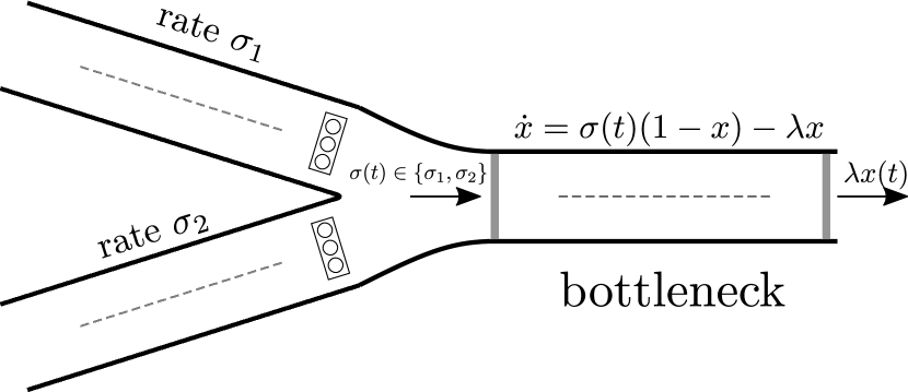
(a)

(b)

Figure 2: Traffic system application illustrating the two strategies. Here $x(t)\in[0,1]$ denotes the occupancy of the bottleneck at time $t$. (a) The inflow rate switches via periodically-varying traffic lights between two flows with rates $\sigma_{1},\sigma_{2}$. At each time, either vehicles in the upper lane or vehicles in the lower lane can enter the bottleneck, but not both. (b) The double lane of each flow is restricted to a single lane and connected directly to the corresponding lane in the bottleneck.

Another application is the ribosome flow model (RFM) [14] which is a deterministic model for ribosome flow along the mRNA molecule. It can be derived via a dynamic mean-field approximation of a fundamental model from statistical physics called the totally asymmetric simple exclusion process (TASEP) [17, 2]. In TASEP particles hop randomly along a chain of ordered sites. A site can be either free or contain a single particle. Totally asymmetric means that the flow is unidirectional, and simple exclusion means that a particle can only hop into a free site. This models the fact that two particles cannot be in the same place at the same time. Note that this generates an indirect coupling between the particles. In particular, if a particle is delayed at a site for a long time then the particles behind it cannot move forward and thus a “traffic jam” of occupied sites may evolve. There is considerable interest in the evolution and impact of traffic jams of various “biological machines” in the cell (see, e.g. [15, 3]).

The RFM is a nonlinear compartmental model with $n$ sites. The state-variable $x_{i}(t)$, $i=1,\dots,n$, describes the normalized density of particles at site $i$ at time $t$, so that $x_{i}(t)=0$ [$x_{i}(t)=1$] means that site $i$ is completely empty [full] at time $t$. The state-space is thus the closed unit cube $[0,1]^{n}$. The model includes $n+1$ parameters $\lambda_{i}$, $i=0,\dots,n$, where $\lambda_{i}>0$ controls the transition rate from site $i$ to site $i+1$. In particular, $\lambda_{0}$ [$\lambda_{n}$] is called the initiation [exit] rate.

The RFM dynamics is described by $n$ first-order ODEs:

$$\dot{x}_{k} =\lambda_{k-1}x_{k-1}(1-x_{k})-\lambda_{k}x_{k}(1-x_{k+1}),\;k=1,\dots,n,$$ (4)

where we define $x_{0}(t)\equiv 1$ and $x_{n+1}(t)\equiv 0$.

In the context of translation, the $\lambda_{i}$’s depend on various biomechanical properties for example the abundance of tRNA molecules that deliver the amino-acids to the ribosomes. A recent paper suggests that cells vary their tRNA abundance in order to control the translation rate [16]. Thus, it is natural to consider the case where the rates are in fact time-varying. Ref. [11] proved, using the fact that the RFM is an (almost) contractive system [13], that if all the rates are jointly $T$-periodic then every solution of the RFM converges to a unique $T$-periodic solution $x^{*}(t)\in(0,1)^{n}$.

Consider the RFM with a time-varying initiation rate $\lambda_{0}(t)=\sigma(t)$ and constant $\lambda_{1},\dots,\lambda_{n}$ such that $\lambda_{i}\gg\sigma(t)$ for all $i\geq 1$ and all $t$. Then we can expect that the initiation rate becomes the bottleneck rate and thus $x_{i}(t)$, $i=2,\dots,n$, converge to values that are close to zero, suggesting that (4) can be simplified to

$$\begin{split}\dot{x}_{1}&=(1-x_{1})\sigma-\lambda_{1}x_{1},\\ \dot{x}_{i}&=\lambda_{i-1}x_{i-1}-\lambda_{i}x_{i},\;\;i\in\{2,\dots,n\},\end{split}$$ (5)

which has the same form as the cascade in Fig. 1.

The remainder of this note is organized as follows. Section II presents a formulation of the problem. Section III describes our main results for the bottleneck system only, with the proof given in Section IV. Section V shows that the same result can be generalized to the cascade.

II Problem Formulation for the Bottleneck System

Fix $T\geq 0$. For any $T$-periodic function $f:\mathbb{R}_{+}\to\mathbb{R}$, let $\operatorname{ave}(f):=\frac{1}{T}\int_{0}^{T}f(s)\mathop{}\!\mathrm{d}s$. Consider first only the bottleneck model (I). A $T$-periodic inflow rate $\sigma(t)$ induces a unique attractive $T$-periodic trajectory that we denote by $x_{\sigma}(t)$ and thus a unique $T$-periodic production rate $w_{\sigma}(t):=\lambda x_{\sigma}(t)$. Thus, after a transient the average production rate is $\operatorname{ave}({w_{\sigma}})$. Now consider the bottleneck system with a constant inflow rate $\bar{\sigma}$. Each trajectory converges to a unique steady-state $\bar{\sigma}/(\lambda+\bar{\sigma})$, and thus to a production rate $\bar{w}:=\lambda\bar{\sigma}/(\lambda+\bar{\sigma})$.

The question we are interested in is: what is the relation between $\bar{w}$ and $\operatorname{ave}(w_{\sigma})$? To make this a “fair” comparison we consider inflow rates from the set $S_{\bar{\sigma},T}$ that includes all the admissible rates $\sigma(t)$ that are $T$-periodic and satisfy $\operatorname{ave}(\sigma)=\bar{\sigma}$. We note that this problem is related to periodic optimal control [18, 19] where the goal is to find an optimal control $u$ under the constraint that $x(T,u)=x(0)$, yet without the additional constraint enforcing that the average on the control is fixed.

We call $\sup_{\sigma\in S_{\bar{\sigma},T}}{\operatorname{ave}(w_{\sigma})}/{\bar{w}},$ where the $\sup$ is with respect to all the (non-trivial) rates in $S_{\bar{\sigma},T}$, the periodic gain of the bottleneck over $S_{\bar{\sigma},T}$.

Indeed, one can naturally argue that the average production rate over a period, rather than the instantaneous value, is the relevant quantity. Then a periodic gain $>1$ implies that we can “do better” using periodic rates. A periodic gain one implies that we do not lose nor gain anything with respect to the constant rate $\sigma(t)\equiv\bar{\sigma}$. A periodic gain $<1$ implies that for any (non-trivial) periodic rate the average production rate is lower than the one obtained for constant rates. This implies that entrainment always incurs a cost, as the production rate for constant rates is higher.

In this paper, we study the periodic gain with respect to inflows that belong to a subset $B_{\bar{\sigma},T}\subset S_{\bar{\sigma},T}$ that is defined as follows. Fix $\sigma_{2}>\bar{\sigma}>\sigma_{1}>0$ such that $(\sigma_{1}+\sigma_{2})/2=\bar{\sigma}$. Let $\sigma(t)$ be any measurable function satisfying $\operatorname{ave}(\sigma)=\bar{\sigma}$ and $\sigma(t)\in\{\sigma_{1},\sigma_{2}\}$, or $\sigma(t)\equiv\bar{\sigma}$. We will actually allow $\sigma$ to be a combination of the two under a specific condition to be explained below.

Since the system entrains to a periodic signal, it is sufficient to consider it on the compact interval $[0,T]$. The entrained occupancy is periodic, hence we need to enforce the condition $x(0)=x(T)$.

For $\sigma(t)\in\{\sigma_{1},\sigma_{2}\}$ the bottleneck system switches between two linear systems:

$$\dot{x}=\sigma_{1}-(\sigma_{1}+\lambda)x,\quad\dot{x}=\sigma_{2}-(\sigma_{2}+\lambda)x.$$

If $\sigma(t)\equiv\bar{\sigma}$ then

$$\dot{x}=\tfrac{\sigma_{1}+\sigma_{2}}{2}(1-x)-\lambda x,$$ (6)

adding the constraint $x(0)=x(T)$, this implies that $x(t)\equiv\tfrac{\bar{\sigma}}{\bar{\sigma}+\lambda}$.

In general, we can consider $\sigma(t)\in\{\sigma_{1},\bar{\sigma},\sigma_{2}\}$ but to have a meaningful combination the occupancy must be constant when $\sigma(t)=\bar{\sigma}$. In other words, $\sigma(t)=\bar{\sigma}$ implies that $x(t)=\tfrac{\bar{\sigma}}{\bar{\sigma}+\lambda}$. Hence the set of admissible inflows is defined as follows:

$$B_{\bar{\sigma},T} :=\{\sigma(t)\!\in\!\{\sigma_{1},\bar{\sigma},\sigma_{2}\}|\textstyle\operatorname{ave}(\sigma)=\bar{\sigma},\sigma(t)\!=\!\sigma(t+T),$$

$$\text{ and }\sigma(t)=\bar{\sigma}\text{ implies that }x(t)=\bar{\sigma}/(\lambda+\bar{\sigma})\}.$$

Our objective is to study the following quantity:

$$J(\sigma(t)):=\operatorname{ave}(\lambda x_{\sigma})/(\frac{\lambda\bar{\sigma}}{\bar{\sigma}+\lambda}),$$

over $\sigma(t)\in B_{\bar{\sigma},T}$. Here $\frac{\lambda\bar{\sigma}}{\bar{\sigma}+\lambda}$ is the outflow for the constant input $\sigma(t)=\bar{\sigma}$, and $\operatorname{ave}(\lambda x_{\sigma})$ is the outflow along the unique globally attracting periodic orbit corresponding to the periodic switching strategy.

III Periodic Gain of the Bottleneck System

The main result of this section can be stated as follows:

Theorem 1.

Consider the bottleneck system (I). If $\sigma\in B_{\bar{\sigma},T}$ then $J(\sigma)\leq 1$.

Thus, a constant inflow cannot be outperformed by a periodic one.

Example 1.

Consider a bottleneck system with $\lambda=1$ and switched inflows $\sigma(t)$ satisfying $\operatorname{ave}(\sigma)=1$. Note that for the constant inflow $\sigma(t)\equiv 1$ the output converges to $w_{\sigma}(t)\equiv 1/2$, so $\operatorname{ave}(w_{\sigma})=1/2$. Fig. 3(a) depicts a histogram of the averaged outflow for randomly generated switching signals in $B_{\bar{\sigma},T}$. The mean performance for the switching laws is $20\%$ lower than that achieved by the constant inflow.

It follows from averaging theory [7][Ch. 10] or using the Lie-Trotter product formula [6] that it is possible to approximate the effect of a constant inflow with any desired accuracy using a sufficiently fast switching law, but such a switching law is not practical in most applications.

Fig. 3(b) shows a scatter plot of the average outflow for a bottleneck system with $\lambda=1$ and different values of $\bar{\sigma}$. It may be seen that it is harder to approach the performance of the constant inflow for higher $\bar{\sigma}$.

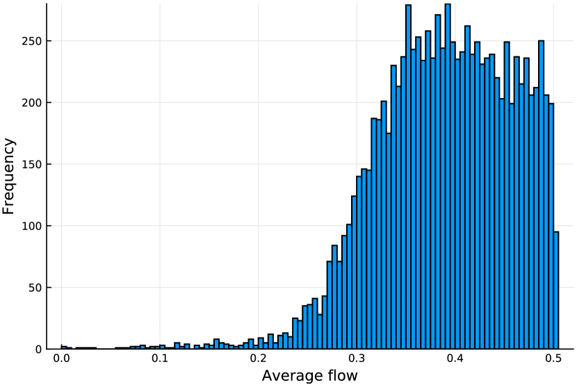
(a)

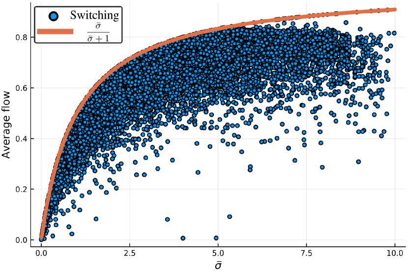
(b)

Figure 3: Performance of the switching policy: (a) Histogram of achievable average outflow rate with $\bar{\sigma}=1$, $\lambda=1$. (b) Scatter plot with $\lambda=1$.

IV Proof of Theorem 1

It is useful to parametrize the class of admissible inflows for a given average $\bar{\sigma}$ as follows:

$$\sigma(t)=\bar{\sigma}+\varepsilon\alpha(t),$$ (7)

where $\alpha(t)$ is measurable, $\operatorname{ave}(\alpha)=0$, $\alpha(t)\in\{-1,0,1\}$ for almost all $t\in[0,T]$, and $0\leq\varepsilon\leq\bar{\sigma}$. Note that $\alpha(t)=1$ [$\alpha(t)=-1$] corresponds to $\sigma(t)=\sigma_{1}$ [$\sigma(t)=\sigma_{2}$], while $\alpha(t)=0$ corresponds to the constant inflow $\sigma(t)=\bar{\sigma}=(\sigma_{1}+\sigma_{2})/2$. Recall that for every choice of $\sigma(t)$ we let $x_{\sigma}$ denote the unique solution of (I) that satisfies $x(0)=x(T)$.

IV-A Finite Number of Switchings

A set $E\subset[0,T]$ is said to be elementary if it can be written as a finite union of open, closed, or half-open intervals. For a given $\alpha$, define $E^{+}:=\{t|\alpha(t)=1\}$, $E^{-}:=\{t|\alpha(t)=-1\}$, and $E^{0}:=\{t|\alpha(t)=0\}$. Then $\alpha(t)$ is said to have a finite number of switchings if $E^{+}$, $E^{-}$, and $E^{0}$ are elementary sets.

We are ready to state the next proposition:

Proposition 2.

Suppose that $\sigma(t)$ satisfies (7) with $\varepsilon>0$, $\alpha(t)$ has a finite number of switchings, and $\mu(E^{0})<T$, where $\mu$ denotes the Lebesgue measure. Then, $J(\sigma)<1.$

To prove this we require three simple auxiliary results that we state as lemmas for easy reference.

Lemma 3.

Consider the scalar system $\dot{x}(t)=a-bx(t)$ with $x(t_{0})=x_{0}$. Pick $t_{1}\geq t_{0}$, and let $x_{1}:=x(t_{1})$. Then:

$$b\int_{t_{0}}^{t_{1}}x(t)\mathop{}\!\mathrm{d}t=a(t_{1}-t_{0})+x_{0}-x_{1}.$$ (8)

Proof.

The solution at time $t$ of the scalar equation satisfies

$$bx(t)=be^{-b(t-t_{0})}x_{0}+a\Big{(}1-e^{-b(t-t_{0})}\Big{)},$$ (9)

and integrating yields

$$b\int_{t_{0}}^{t}x(t)\mathop{}\!\mathrm{d}t=a(t_{1}-t_{0})+bx_{0}-bx_{0}e^{-b(t-t_{0})}-a\Big{(}1-e^{-b(t-t_{0})}\Big{)}$$

and combining this with (9) for $t=t_{1}$ gives (8). ∎

Lemma 4.

For any $a,b>0$ we have

$$\frac{(1-e^{-a})(1-e^{-b})}{1-e^{-(a+b)}}<\frac{ab}{a+b}.$$ (10)

Proof.

Let $f(a,b):=\frac{1-e^{-(a+b)}}{(1-e^{-a})(1-e^{-b})}-\frac{1}{a}-\frac{1}{b}$. The inequality is proved if we show that $f(a,b)>0$ for all $a,b>0$. Note that $\lim_{(a,b)\downarrow(0,0)}f(a,b)=0$. Differentiating $f$ with respect to $a$ yields $\frac{\partial f}{\partial a}=\frac{1}{a^{2}}+\frac{1}{2-2\cosh(a)}.$ Using the Taylor series of $\cosh(a)$ we find that $2\cosh(a)-2>a^{2}$, so $\partial f/\partial a>0$. Similarly, $\partial f/\partial b>0$. Hence, $f$ increases in all directions in the positive orthant. ∎

Lemma 5.

Consider the scalar systems $\dot{x}_{i}(t)=a_{i}-b_{i}x_{i}(t)$, $i=1,2$, with $b_{i}>0$. Suppose that there exist $v,w\in\mathbb{R}$ and $t_{1},t_{2}>0$ such that for $x_{1}(0)=v$ and $x_{2}(0)=w$, we have $x_{1}(t_{1})=w$ and $x_{2}(t_{2})=v$. Then

$$w-v=(c_{1}-c_{2})\frac{(1-e^{-b_{1}t_{1}})(1-e^{-b_{2}t_{2}})}{1-e^{-b_{1}t_{1}-b_{2}t_{2}}},$$ (11)

where $c_{i}:=a_{i}/b_{i}$, $i=1,2$. If, furthermore, $c_{1}>c_{2}$ then

$$w-v<(c_{1}-c_{2})b_{1}t_{1}b_{2}t_{2}/(b_{1}t_{1}+b_{2}t_{2}).$$ (12)

Proof.

We know that $w=e^{-b_{1}t_{1}}v+c_{1}(1-e^{-b_{1}t_{1}})$ and that $v=e^{-b_{2}t_{2}}w+c_{2}(1-e^{-b_{2}t_{2}})$. Combining these equations yields

$$w =c_{1}(1-e^{-b_{1}t_{1}})+e^{-b_{1}t_{1}}\left(c_{2}(1-e^{-b_{2}t_{2}})+e^{-b_{2}t_{2}}w\right),$$

$$v =c_{2}(1-e^{-b_{2}t_{2}})+e^{-b_{2}t_{2}}\left(c_{1}(1-e^{-b_{1}t_{1}})+e^{-b_{1}t_{1}}v\right),$$

and this gives (11). If $c_{1}>c_{2}$ then Lemma 4 yields (12). ∎

Going back to our problem, note that the system (I) with an input $\sigma$ given in (7) is a switched linear system [9] which switches between three linear systems in the form $\dot{x}=a_{z}-b_{z}x$, $z\in\{-,0,+\}$ (see Fig. 4), with

$$a_{-} :=\bar{\sigma}-\varepsilon b_{-}:=\bar{\sigma}+\lambda-\varepsilon,$$ , (13)

$$a_{0} :=\bar{\sigma}, b_{0}:=\bar{\sigma}+\lambda,$$

$$a_{+} :=\bar{\sigma}+\varepsilon b_{+}:=\bar{\sigma}+\lambda+\varepsilon,$$ ,

corresponding to $\alpha(t)=-1$, $0$, and $1$, respectively. We refer to the corresponding arcs as a $z$-arc, with $z\in\{-,0,+\}$. Note that $b_{+}>b_{0}>b_{-}>0$. Letting $c_{i}:=a_{i}/b_{i}$, we also have

$$c_{+}-c_{-} =\frac{2\lambda\varepsilon}{(\bar{\sigma}+\lambda+\varepsilon)(\bar{\sigma}+\lambda-\varepsilon)}>0.$$ (14)

Recall that along a $0$-arc the solution satisfies $x(t)\equiv c_{0}$. Since $x(T)=x(0)$, the other arcs form a loop with a finite number of sub-loops. Observe that the $(+)$-arcs and the $(-)$-arcs can be paired: if a $(+)$-arc traverses from $x(t)=x_{i}^{-}$ to $x(t+t^{+}_{i})=x_{i}^{+}$, then there must be a $(-)$-arc that traverses back from $x_{i}^{+}$ to $x_{i}^{-}$ (see Fig. 4). Hence any trajectory can be partitioned into $n$ arcs with $x_{0}^{-},x_{0}^{+},x_{1}^{-},x_{1}^{+},...,x_{n}^{-},x_{n}^{+}>0$ as the switching points. Let $t_{i}^{+}$ [$t_{i}^{-}$] be the time spent on the $i$’th $(+)$- arc [$(-)$-arc], respectively. Combining this with the assumption that $\alpha(t)$ has a finite number of switches and (8) implies that

$$\int_{0}^{T}x(t)\mathop{}\!\mathrm{d}t =\int_{t\in E^{0}}x(t)\mathop{}\!\mathrm{d}t+\int_{t\in E^{+}}x(t)\mathop{}\!\mathrm{d}t+\int_{t\in E^{-}}x(t)\mathop{}\!\mathrm{d}t$$

$$=c_{0}\mu(E^{0})+\sum_{i=1}^{n}\left(c_{+}t_{i}^{+}+(x_{i}^{-}-x_{i}^{+})/b_{+}\right)$$

$$+\sum_{i=1}^{n}\left(c_{-}t_{i}^{-}+(x_{i}^{+}-x_{i}^{-})/b_{-}\right).$$

Thus,

$$\int_{0}^{T}x(t)\mathop{}\!\mathrm{d}t =c_{0}\mu(E^{0})+c_{+}\mu(E^{+})+c_{-}\mu(E^{-})$$

$$+(\frac{1}{b_{-}}-\frac{1}{b_{+}})\sum_{i=1}^{n}(x_{i}^{+}-x_{i}^{-}).$$

It follows from (12) that $x_{i}^{+}-x_{i}^{-}<(c_{+}-c_{-})\frac{b_{+}t_{i}^{+}b_{-}t_{i}^{-}}{b_{+}t_{i}^{+}+b_{-}t_{i}^{-}},$ so

$$\int_{0}^{T}x(t)\mathop{}\!\mathrm{d}t =c_{0}\mu(E^{0})+c_{+}\mu(E^{+})+c_{-}\mu(E^{-})$$

$$+(c_{+}-c_{-})({b_{+}}-{b_{-}})\sum_{i=1}^{n}\frac{t_{i}^{+}t_{i}^{-}}{b_{+}t_{i}^{+}+b_{-}t_{i}^{-}}.$$ (15)

Let $t_{i}:=t_{i}^{+}+t_{i}^{-}$ and $\delta_{i}:=t_{i}^{+}-t_{i}^{-}$. Then

$$\frac{t_{i}^{+}t_{i}^{-}}{b_{+}t_{i}^{+}+b_{-}t_{i}^{-}} =\frac{(t_{i}+\delta_{i})(t_{i}-\delta_{i})}{4(b_{0}t_{i}+\varepsilon\delta_{i})}$$

$$=\frac{t_{i}^{2}-\delta_{i}^{2}}{4b_{0}(t_{i}+(\varepsilon\delta_{i}/b_{0}))}$$

$$<\frac{1}{4b_{0}}(t_{i}-(\varepsilon\delta_{i}/b_{0})),$$ (16)

where the last inequality follows from the fact that $b_{0}^{2}=(\bar{\sigma}+\lambda)^{2}>\varepsilon^{2}$. Thus,

$$\sum_{i=1}^{n}\frac{t_{i}^{+}t_{i}^{-}}{b_{+}t_{i}^{+}+b_{-}t_{i}^{-}} <\frac{1}{4b_{0}}\sum_{i=1}^{n}t_{i}$$

$$=(\mu(E^{-})+\mu(E^{+}))/(4b_{0}),$$

and plugging this in (IV-A) yields

$$\int_{0}^{T}x(t)\mathop{}\!\mathrm{d}t <c_{0}\mu(E^{0})+c_{+}\mu(E^{+})+c_{-}\mu(E^{-})$$ (17)

$$+(c_{+}-c_{-})({b_{+}}-{b_{-}})(\mu(E^{-})+\mu(E^{+}))/(4b_{0}).$$

Since $\operatorname{ave}(\alpha)=0$, $\mu(E^{+})-\mu(E^{-})=0$, and combining this with the fact that $\mu(E^{+})+\mu(E^{-})+\mu(E^{0})=T$ yields

$$\mu(E^{+})=\mu(E^{-})=(T-\mu(E^{0}))/2.$$

Plugging this and (13) in (17) and simplifying yields $\int_{0}^{T}x(t)\mathop{}\!\mathrm{d}t<\frac{\bar{\sigma}}{\bar{\sigma}+\lambda}T,$ and this completes the proof of Prop. 2.

We note in passing that one advantage of our explicit approach is that by using a more exact analysis in (IV-A) it is possible to derive exact results on the “loss” incurred by using a non-constant inflow.

Figure 4: A trajectory of the switched system with $x(0)=x(T)$ traverses a loop in the $(\dot{x},x)$-plane. The upper [lower] line corresponds to $\alpha(t)=1$ [$\alpha(t)=-1$]. There is no line for the case $\alpha(t)=0$ since we assume that the corresponding trajectory stays at a fixed point in the $(x,\dot{x})$ plane.

IV-B Arbitrary Switchings

For two sets $A,B$ let $A\Delta B:=(A\setminus B)\cup(B\setminus A)$ denote the symmetric difference of the sets. To prove Thm. 1, we need to consider a measurable signal $\alpha(t)$ in (7). We use the following characterization of measurable sets:

Lemma 6.

[8] Let $E\subset[0,T]$. Then $E$ is measurable if and only if for every $\varepsilon>0$ there exists an elementary set $B_{\varepsilon}\subset[0,T]$ such that $\mu(E\Delta B_{\varepsilon})<\varepsilon$.

We improve on the lemma above, by the following:

Lemma 7.

Let $E\subset[0,T]$. Then $E$ is measurable if and only if for every $\varepsilon>0$ there exists an elementary set $B_{\varepsilon}\subset[0,T]$ with $\mu(B_{\varepsilon})=\mu(E)$ such that $\mu(E\Delta B_{\varepsilon})<\varepsilon$.

Proof.

Sufficiency is clear. To prove necessity, pick $\varepsilon>0$. By Lemma 6, there exists an elementary set $B_{\varepsilon/2}\subset[0,T]$ such that $\mu(E\Delta B_{\varepsilon/2})<\varepsilon/2$. We can modify the intervals contained in $B_{\varepsilon/2}$ by up to $\varepsilon/2$ to get $B_{\varepsilon}$ with $\mu(B_{\varepsilon})=\mu(E)$ and $\mu(E\Delta B_{\varepsilon})<\varepsilon$. ∎

We generalize Prop. 2 as follows:

Proposition 8.

If $\sigma(t)$ is given as in (7) with $\alpha(t)$ measurable then $J(\sigma)\leq 1$.

Proof.

Let $E^{0},E^{+},E^{-}$ be defined as before. For any $i\geq 1$, let $\varepsilon_{i}:=2^{-i}$. By Lemma 7, there exist elementary sets $E_{i}^{0},E_{i}^{+},E_{i}^{-}$ such that $\mu(E_{i}^{0})=\mu(E^{0})$ and $\mu(E^{0}\Delta E_{i}^{0})<\varepsilon_{i}=2^{-i}$, and similarly for $E_{i}^{+},E_{i}^{-}$. Note that this implies that $\mu(E_{i}^{0})+\mu(E_{i}^{+})+\mu(E_{i}^{-})=T$. For every $i\geq 1$ define

$$\alpha_{i}(t):=\begin{cases}1,&\text{ if }t\in E_{i}^{+},\\ 0,&\text{ if }t\in E_{i}^{0},\\ -1,&\text{ if }t\in E_{i}^{-}.\end{cases}$$

Then $\alpha_{i}(t)$ are elementary simple functions, and $\lim_{i\to\infty}\alpha_{i}(t)=\alpha(t)$ for all $t\in[0,T]$. For each $i$, we can apply Prop. 2 to the periodic solution $x_{\alpha_{i}}$. Now the proof follows from Lebesgue’s bounded convergence theorem [8]. ∎

This completes the proof of Thm. 1.

V Periodic Gain of the Cascade System

We have shown above that a constant inflow outperforms any switched inflow for the bottleneck system which is the first block in Fig. 1. We now show that the result can be generalized if we have a positive linear system after the bottleneck. We first show that the periodic gain of a Hurwitz linear system does not depend on the particular periodic signal, but only on the DC gain of the system.

Proposition 9.

Consider a SISO Hurwitz linear system (I). Let $w$ be a bounded measurable $T$-periodic input. Recall that the output converges to a steady-state $y_{w}$ that is $T$-periodic. Then

$$\frac{1}{T}\int_{0}^{T}y_{w}(t)\mathop{}\!\mathrm{d}t=H(0)\frac{1}{T}\int_{0}^{T}w(t)\mathop{}\!\mathrm{d}t,$$

where $H(s):=c^{T}(sI-A)^{-1}b$ is the transfer function of the linear system.

Thus, the periodic gain of a linear system is the same for any input.

Proof.

Since $w$ is measurable and bounded, $w\in L_{2}([0,T])$. Hence, it can be written as a Fourier series

$$w(t)=\operatorname{ave}(w)+\sum_{i}a_{i}\sin(\omega_{i}t+\phi_{i}).$$

The output of the linear system converges to: $y_{w}(t)=H(0)\operatorname{ave}(w)+\sum_{i}|H(j\omega_{i})|a_{i}\sin(\omega_{i}t+\phi_{i}+\mbox{arg}(H(j\omega_{i}))).$ Each sinusoid in the expansion has period $T$, so $\int_{0}^{T}y_{w}(t)\mathop{}\!\mathrm{d}t=TH(0)\operatorname{ave}(w).$ ∎

If $H(0)=-c^{T}A^{-1}b\geq 0$ (e.g. when the linear system is positive) then and we can extend Thm. 1 to the cascade in Fig. 1:

Theorem 10.

Consider the cascade of (I) and (I) in Fig. 1. If $\sigma\in B_{\bar{\sigma},T}$ then $\frac{1}{T}\int_{0}^{T}y_{\sigma}(t)\mathop{}\!\mathrm{d}t\leq\tfrac{\lambda\bar{\sigma}}{\lambda+\bar{\sigma}}H(0).$

Thus, a constant inflow cannot be outperformed by a switched inflow.

VI Conclusion

We analyzed the performance of a switching control for a specific type of SISO nonlinear system that is relevant in fields such as traffic control and molecular biology.

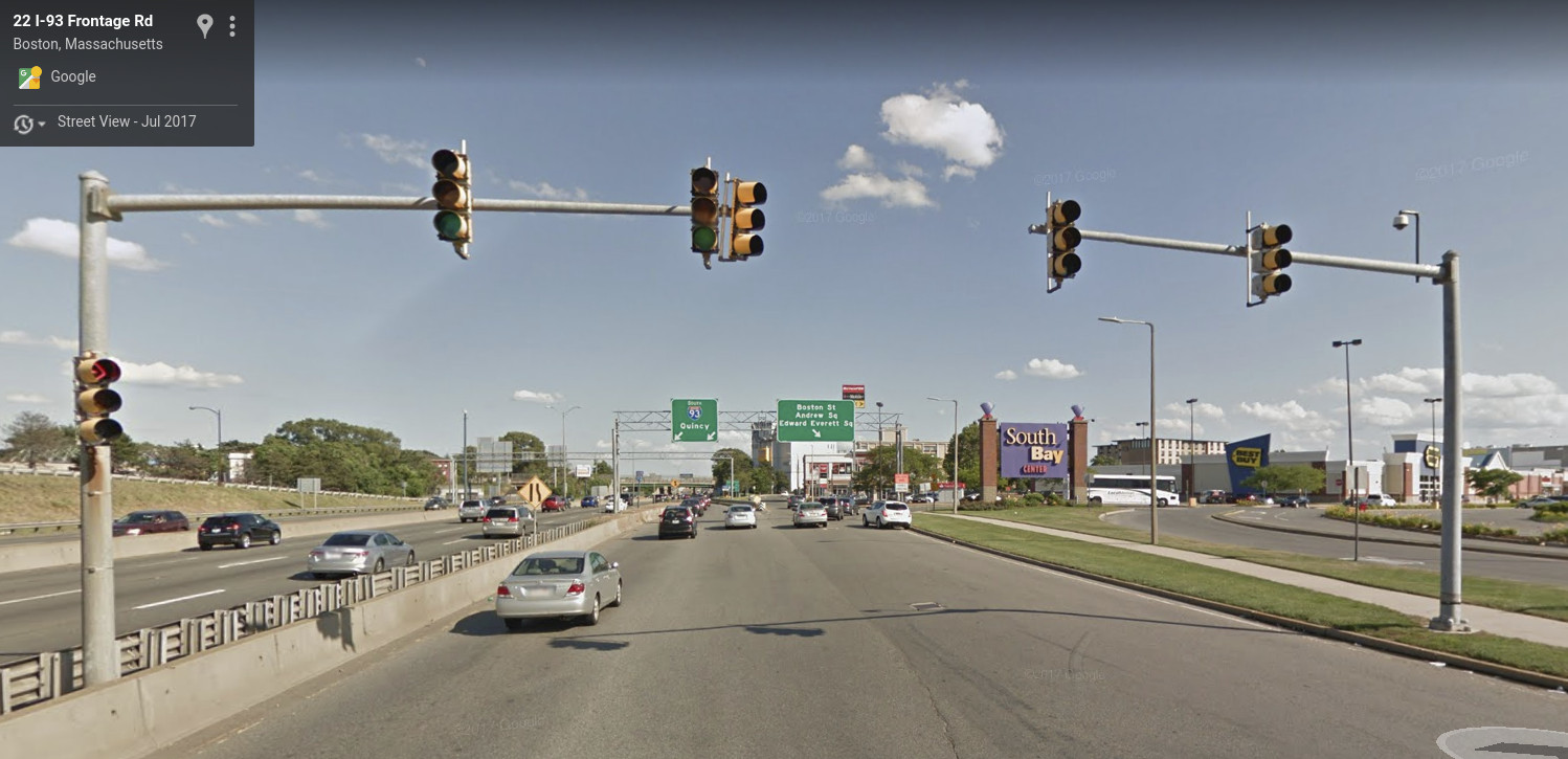
(a)

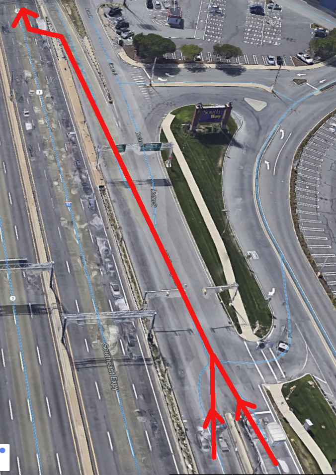
(b)

Figure 5: Example of the switching design in Fig. 2(a) located at an i-93 entrance in Boston, MA (42^∘19’46.8”N 71^∘03’39.7”W). (a) The two traffic lights. (b) The path taken by vehicles to join the i-93 road. (Copyright: Google Earth)

We have shown that a constant inflow outperforms switching inflows with the same average. The performance of the switching inflow can be enhanced by faster switching, but this is not practical in most applications (e.g. traffic systems). Nevertheless, the switching inflow can be found in the real world (Fig. 5), and our analysis shows that, for our model, such design involves a deterioration in the throughput of the system.

The periodic gain may certainly be larger than one for some nonlinear systems and then nontrivial periodic inflows are better than the constant inflow. For example, given the bottleneck system, let $\xi(t):=1-x(t)$. Then we obtain the dual system $\dot{\xi}(t)=\lambda(t)-(\lambda(t)+\sigma(t))\xi(t).$ Defining the output as $w(t):=\lambda\xi(t)$ it follows from Thm. 1 that here a periodic switching cannot be outperformed by a constant inflow.

A natural question then is how can one determine whether the periodic gain of a given nonlinear system is larger or smaller than one. Other directions for further research include analyzing the periodic gain of important nonlinear models like TASEP and the $n$-dimensional RFM. A possible generalization would be to consider a bottleneck-input boundary linear hyperbolic PDE instead of a finite-dimensional system and its application to communication and traffic networks (see e.g. [4]).

References

- [1] Z. Aminzare and E. D. Sontag, “Contraction methods for nonlinear systems: A brief introduction and some open problems,” in Proc. 53rd IEEE Conf. on Decision and Control, Los Angeles, CA, 2014, pp. 3835–3847.
- [2] R. A. Blythe and M. R. Evans, “Nonequilibrium steady states of matrix-product form: a solver’s guide,” J. Phys. A: Math. Gen., vol. 40, no. 46, pp. R333–R441, 2007.
- [3] A. Diament, A. Feldman, E. Schochet, M. Kupiec, Y. Arava, and T. Tuller, “The extent of ribosome queuing in budding yeast,” PLOS Computational Biology, vol. 14, no. 1, p. e1005951, 2018.
- [4] N. Espitia, A. Girard, N. Marchand and C. Prieur “Fluid-flow modeling and stability analysis of communication networks,” in Proc. 20th IFAC World Congress, Toulouse, France, 2017, pp. 4534–4539.
- [5] L. Glass and M. C. Mackey, “A simple model for phase locking of biological oscillators,” J. Math. Biology, 7(4):339–352, 1979.
- [6] B. C. Hall, Lie Groups, Lie Algebras, and Representations: An Elementary Introduction, 2nd ed. Springer, 2015.
- [7] H. K. Khalil, Nonlinear Systems, 3rd ed. Prentice Hall, 2002.
- [8] A. N. Kolmogorov and S. V. Fomin, Introductory Real Analysis. Courier Corporation, 1975.
- [9] D. Liberzon, Switching in Systems and Control. Basel, Switzerland: Birkhäuser, 2003.
- [10] W. Lohmiller and J.-J. E. Slotine, “On contraction analysis for non-linear systems,” Automatica, vol. 34, pp. 683–696, 1998.
- [11] M. Margaliot, E. D. Sontag, and T. Tuller, “Entrainment to periodic initiation and transition rates in a computational model for gene translation,” PLOS ONE, vol. 9, no. 5, p. e96039, 2014.
- [12] M. Margaliot and T. Tuller, “Stability analysis of the ribosome flow model,” IEEE/ACM Trans. Computational Biology and Bioinformatics, vol. 9, no. 5, pp. 1545–1552, 2012.
- [13] M. Margaliot, T. Tuller, and E. D. Sontag, “Checkable conditions for contraction after small transients in time and amplitude,” in Feedback Stabilization of Controlled Dynamical Systems: In Honor of Laurent Praly, N. Petit, Ed. Cham, Switzerland: Springer International Publishing, 2017, pp. 279–305.
- [14] S. Reuveni, I. Meilijson, M. Kupiec, E. Ruppin, and T. Tuller, “Genome-scale analysis of translation elongation with a ribosome flow model,” PLOS Computational Biology, vol. 7, no. 9, p. e1002127, 2011.
- [15] J. L. Ross, “The impacts of molecular motor traffic jams,” Proceedings of the National Academy of Sciences, vol. 109, no. 16, pp. 5911–5912, 2012.
- [16] M. Torrent, G. Chalancon, N. S. de Groot, A. Wuster, and M. Madan Babu, “Cells alter their tRNA abundance to selectively regulate protein synthesis during stress conditions,” Science Signaling, vol. 11, no. 546, 2018.
- [17] R. K. P. Zia, J. Dong, and B. Schmittmann, “Modeling translation in protein synthesis with TASEP: A tutorial and recent developments,” J. Stat. Phys., vol. 144, pp. 405–428, 2011.
- [18] S. Bittanti, G. Fronza, and G. Guardabassi, “Periodic control: A frequency domain approach,” IEEE Trans. Automat. Contr., vol. 18(1), pp. 33–38, 1973.
- [19] E. G. Gilbert, “Optimal periodic control: A general theory of necessary conditions,” SIAM J. Control Optim., vol. 15(5), pp. 717–746, 1977.