Networks and Hierarchies: How Amorphous Materials Learn to Remember

Abstract

We consider the slow and athermal deformations of amorphous solids and show how the ensuing sequence of discrete plastic rearrangements can be mapped onto a directed network. The network topology reveals a set of highly connected regions joined by occasional one-way transitions. The highly connected regions include hierarchically organized hysteresis cycles and sub-cycles. At small to moderate strains this organization leads to near-perfect return point memory. The transitions in the network can be traced back to localized particle rearrangements (soft-spots) that interact via Eshelby-type deformation fields. By linking topology to dynamics, the network representations provides new insights into the mechanisms that lead to reversible and irreversible behavior in amorphous solids.

A wide variety of condensed matter systems exhibit memory effects, since their present states are a result of their past history, which is encoded in their structure. Often all or at least part of such histories may be inferred from measurements Keim et al. (2019). Examples include shape memory materials, disordered magnets, spin glasses, structural glasses and granular matter, and magnetic and phase change memory devices. In particular, memory effects in cyclically driven (sheared) amorphous solids and colloidal suspensions have been recently investigated through computer simulations, experiments and theoretical modeling Keim et al. (2019); Paulsen et al. (2014); Fiocco et al. (2014, 2015); Mungan and Witten (2019). For small to moderate deformations, upon repeated cyclic loading, after a transient, these systems reach limit cycles in which they traverse the same sequence of states during each subsequent cycle Corte et al. (2008); Keim and Nagel (2011); Keim et al. (2013); Regev et al. (2013); Fiocco et al. (2013); Paulsen et al. (2014); Keim and Arratia (2014); Fiocco et al. (2014); Regev et al. (2015); Fiocco et al. (2015); Hima Nagamanasa et al. (2014); Kawasaki and Berthier (2016); Leishangthem et al. (2017); Adhikari and Sastry (2018); Keim et al. (2018, 2019); Regev and Lookman (2019); Bandi et al. (2018); Libál et al. (2012); Mungan and Witten (2019).

In contrast, systems obeying the “no-passing” property, an ordering of states that is preserved by the dynamics, exhibit limit cycles immediately, i.e. without any transients. Examples include systems with either no coupling at all, such as the Preisach model Preisach (1935) or systems that have only positive couplings, such as depinning models and the random field Ising model Middleton (1992). Theoretical studies show that “no-passing” is a sufficient condition for return point memory (RPM) Middleton (1992); Sethna et al. (1993), wherein a system remembers the values at which the direction of an external driving field are reversed. Negative couplings can break the no passing property. Indeed, in amorphous solids units of plastic deformation – referred to as shear transformation zones Argon (1979); Falk and Langer (1998) or soft spots – Manning and Liu (2011), induce long-range quadrupolar displacement fields of the type associated with Eshelby inclusions Eshelby (1957); Maloney and Lemaître (2006), that provide equally many positive and negative couplings with other locations of plastic rearrangements. The no-passing property must be violated in these systems, and one therefore expects that return point memory should not hold either. Yet there are experimental as well as numerical findings that are highly reminiscent of return point memory Keim et al. (2018, 2019). Understanding memory effects in amorphous solids appears thus to require a deeper knowledge of the organization of states and transitions among these than is presently available. We develop such insights by introducing a novel method that maps the deformation paths of amorphous systems to directed graphs. As recently shown by one of us, RPM is a well-defined property of such graphs that is easily identified Mungan and Terzi (2019). We construct such graphs from simulations of sheared amorphous solids. Surprisingly, despite the fact that the coupling is not strictly positive, which precludes no-passing, these systems show remarkably accurate, if not perfect, return point memory along with a near-perfect hierarchy of cycles and sub-cycles. We trace the smallest loops to local bistable hysteretic regions undergoing pure shear displacements Manning and Liu (2011). The relatively rare cases in which RPM is violated can be associated with certain destabilizing soft-spot interactions that lead to plastic events which provide one-way escapes from limit-cycles (“rabbit-holes”).

We simulate a two dimensional binary mixture of equal numbers of small and large particles (512 each) with size ratio 1.4, interacting with a radially symmetric potential (described in Lerner and Procaccia (2009); Regev et al. (2013)). Energy minimum structures obtained from liquid configurations are subjected to small strain steps of $\pm\Delta\gamma=10^{-4}$ followed by energy minimization, implementing the athermal quasi-static (AQS) protocol used in previous studies. We thus always consider configurations at mechanical equilibrium at any given strain. Starting with a configuration at some strain $\gamma$, upon increasing strain, the configuration will deform elastically until a critical strain $\gamma^{+}$ is reached where a plastic rearrangement of particles occurs. Likewise, starting from the same initial configuration, and decreasing the strain, the system undergoes elastic deformations until a critical strain $\gamma^{-}<\gamma$ is reached, when another plastic event occurs .

We regard the set of stable configurations, whose members are continuously transformable into each other under strain changes, as one abstract state which we call a mesostate. The strain interval $\gamma^{-}<\gamma<\gamma^{+}$ over which purely elastic deformations are possible we call the stability range $\gamma^{\pm}$ of a mesostate. When a configuration of the mesostate is sheared to $\gamma^{+}$, a plastic event leads to a configuration, which belongs to a new mesostate. Likewise, straining in the negative direction to $\gamma^{-}$ leads to a plastic transition to a configuration belonging to a third mesostate. The potential energy associated with mesostates and their transitions is sketched in Fig 1(a). The mesostate transitions are history-independent: whenever the system is in a configuration $a$ belonging to mesostate $A$, it must transit to the same pair of mesostates when the strain is increased to $\gamma^{+}(A)$, or reduced to $\gamma^{-}(A)$. These transitions can be represented as a graph where each node is a mesostate $A$ and two outgoing arrows specify the transitions to the mesostates that are reached after the plastic events at $\gamma^{\pm}(A)$ Mungan and Terzi (2019); Mungan and Witten (2019). These transitions, together with their thresholds $\gamma^{\pm}$ suffice to prescribe the AQS response of the system to arbitrary shearing protocols Mungan and Terzi (2019). We use the numerical simulations to assemble a catalog of mesostates. For each state $A$ we record the values of $\gamma^{\pm}(A)$ and specify the two mesostates into which $A$ is mapped when $\gamma=\gamma^{\pm}(A)$. We limit our catalog to mesostates that can be reached from a chosen reference state $O$ in at most $\ell=25$ transitions and construct a transition graph from a reference configuration $O$ at zero-strain. A sample graph with $\mathcal{N}=1416$ mesostates is shown in Fig. 1 (b) and exhibits tree-like features as well as regions with high interconnections . A detailed discussion of general features will be done elsewhere Regev et al. (2018). Transitions under forward (positive) and backward (negative) shear are denoted by gray or orange arrows respectively. Certain transitions are emphasized by black and red highlights, respectively .

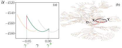
Figure 1: Mesostates and Transition Graphs (a) Potential energy $\mathcal{U}$ of particle configurations associated with an initial mesostate (green segment) and the two mesostates it transits into when the applied strain $\gamma$ ($x$-axis) becomes $\gamma^{\pm}$. (b) The network generated starting from a zero-strain configuration $O$. The $1$ cycle transient and limit-cycle (between $X$ and $Y$) for $\gamma=0.05$ are marked in black and red.

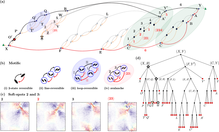
Figure 2: State transition graph of the $\gamma_{\rm max}=0.05$ limit-cycle. (a) Detailed view of the mesostate transitions associated with the $0.05$ limit-cycles depicted in Fig. 1 (b). Transitions out of the endpoints $X$ and $Y$ are marked as green triangles and will be ignored. Regions of interest have colored backgrounds and refer to (b) and Fig. 3(c). (b) Network motifs involving one and two soft-spots, (i) and (ii) - (iv), respectively. Soft-spots are shown as black ellipses with states corresponding to their orientation. Motif background color and transition pattern highlighted in (a) coincide. (c) The particle displacements associated with the transitions of the avalanche motif in (iv) and (a). (d) Tree representation of the hierarchy of loops and sub-loops making up the limit cycle shown in (a). Refer to text for details.

To understand a typical limit-cycle in terms of the transition graph, starting in $O$ and using our catalog we can trace out the set of mesostates obtained for periodic shear with strain $0\to\gamma_{\rm max}\to-\gamma_{\rm max}\to 0\to\cdots$. Fig 2(a) shows the mesostates and transitions of the $\gamma_{\rm max}=0.05$ limit cycle and its vicinity. With the limit-cycle in state $X$ at $-\gamma_{\rm max}$ and as the strain increases, the system undergoes a sequence of plastic events (black arrows), passing through the mesostates $O^{\prime},P,Q^{\prime},Q,R,A^{\prime},Y^{\prime}$ and reaching the upper endpoint $Y$ at $+\gamma_{\rm max}$. Subsequently reducing the strain back to $-\gamma_{\rm max}$, the dynamics follows the red arrows, passing through $A,B,C,C^{\prime},E,F$ and eventually returning to the lower endpoint $X$. Reversing the shearing direction anywhere along the decreasing (red) branch will lead to the upper end point $Y$. Likewise, reversal along the increasing (black) branch leads to $X$, except for $R$, where the strain reversal leads via $Z$ to an exit from the loop. Trajectories that return to an endpoint upon a strain reversal necessarily form sub-cycles. For example the pair of states $(C,Y)$ are the endpoint of a sub-cycle. In fact, a hierarchical structure of cycles nested within cycles is apparent. This structure is highly reminiscent of return point memory, as discussed below.

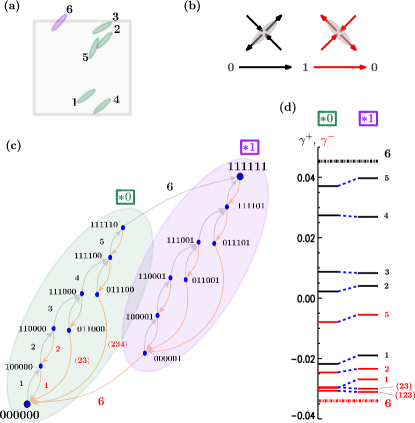
Figure 3: Limit-cycles as interacting soft-spot systems. (a) Location and label of the six soft spots in the sample that produce the plastic events of the cycle $(C^{\prime},Y)$ in Fig. 2(a). (b) Schematic description of particle displacements during a state change of a soft spot $0\rightarrow 1$ and back, $1\rightarrow 0$. (c) State transitions in the sub-cycles marked $\bf{[*0]}$ and $\bf{[*1]}$. The two cycles are topologically identical and the transitions in each are due to the same 5 soft spots. Transition from one cycle to the other occurs via the state change of a sixth soft spot. Labels next to the transitions in sub-cycle $\bf{[*0]}$ indicate the soft spots involved (same in sub-cycle $\bf{[*1]}$). Binary strings next to each mesostate indicate the individual states of soft-spots. The transitions marked $(23)$ and $(234)$ are avalanches. (d) “Spectroscopic” plot showing the non-monotonic changes in the switching strains $\gamma^{\pm}$ of soft-spot $1-5$, depending on the state of $\#6$. The horizontal lines indicate the values of the switching strains along with the soft spots involved.

The state transition graph of Fig. 2(a) has several recurring network transition patterns or “motifs”, which we depict in panels (i) - (iv) of Fig 2(b). Inspecting the corresponding particle displacements, we see these motifs arising from transitions, with hysteresis, between two states in localised soft spots. The simplest motif is a reversible transition which involves only one soft spot, Fig. 2(b)(i), such as transitions between states $X$ and $O^{\prime}$ or $O^{\prime}$ and $P$ in Fig 2(a). Next, transitions between $X$ and $P$ turn out to involve two soft-spots that change states one after the other as the strain is increased, or subsequently reduced, leading to a line reversible motif, depicted in Fig 2(b)(ii). Another pattern involves two soft-spots which change their states in the same order during an increase or decrease of strain, leading to the loop reversible motif, Fig 2(b)(iii), e.g. the pattern highlighted in blue in Fig 2(a) involving transitions between $T^{\prime},Q^{\prime},Q,$ and $T$. The last, and perhaps most important motif we observe is due to avalanches. Here two or more two-level systems change states one after the other in one direction of strain, but return together to their initial state upon strain reversal, see Fig 2(b)(iv). The region highlighted in pink in Fig 2(a)) as well as the transitions of Fig 2(a) marked $(23)$ and $(234)$ in the sub-cycle $(C^{\prime},Y^{\prime})$ are avalanches. The presence of avalanches implies that soft spots interact with each other. The state of one soft spot can enable or even disable the ability of another soft spot to switch states. The interactions between soft spots are mediated via an Eshelby-like quadrupolar deformation fields, arising from a change of state of one soft spot during a plastic event. They are shown in Fig 2(c) for the four transitions making up the avalanche motif of Fig 2(b)(iv). Here the soft-spot labeled 2 can switch its state back and forth when soft spot 3 remains in one state. However after 3 also changes its state, both 2 and 3 reverse their states together. Another, rather striking, example for such soft-spot interactions is the pair of loops $(C^{\prime},Y^{\prime})$ and $(C,Y)$ in Fig. 2(a), shaded in green, which have identical topology. Transitions in these loops are due to the same $5$ soft spots, including $\#2$ and $\#3$ of Fig. 2(c). We have labeled them accordingly as $1$–$5$ and marked the transitions they generate in loop $(C^{\prime},Y^{\prime})$. The change from one loop to the other is due to a sixth soft spot. The locations in the sample of all six soft spots are marked in Fig. 3(a). Panels (b) - (c) of Fig. 3 illustrate the binary encoding of the mesostates in terms of the states of each soft spot (refer to caption for further details). Fig. 3 (d) depicts the non-monotonic changes of switching strains $\gamma^{\pm}_{i}$ for soft spots $1-5$ in dependence on the state soft-spot $6$. This non-monotonic behavior is consistent with the quadrupolar nature of the elastic deformation (note that this is a more complicated example of loop-reversible dynamics).

The property of the system to return to the cycle’s endpoints upon reversal of the forcing, when starting from a mesostate on a limit-cycle or on any of its sub-cycles, is called loop return point memory $(\ell$RPM). It is a generalization of RPM that does not require the existence of the no-passing property Mungan and Terzi (2019). The limit-cycle $(X,Y)$ of Fig 2(a) would have $\ell$RPM, if two transitions were rewired: the orange arrow from $Z$ should point to $X$, while the gray arrow from $W$ should lead to $R$. The first rewiring ensures that a strain reversal at $R$ leads to the lower endpoint $X$, while the second rewiring makes sure that in any sub-cycle of the now corrected cycle $(R,X)$ strain reversals lead to its endpoints $X$ and $R$. With 2 RPM violating transitions out of 84, the limit-cycle of Fig 2(a) exhibits near perfect RPM In fact, we have observed near-perfect RPM in limit cycles for strain amplitudes up to at least $\gamma_{\rm max}=0.0722$; see Section S2.2 in Supplemental Material for an example. In Fig 2 (d) we display the tree representation of the loop hierarchy introduced in Mungan and Terzi (2019) for the $\gamma_{\rm max}=0.05$ limit-cycle whose endpoints are $(X,Y)$. Nodes of this tree represent cycles. Starting from the root $(X,Y)$, each generation represents a partition of the parent cycles into two or three sub-cycles. The tree thus depicts the hierarchy of cycles under this partition. In a network with perfect return point memory, this will be a strict genealogical tree with each child loop having precisely one parent loop. The RPM violations alter this structure. We have indicated the loops involved in RPM violations by gray diamonds, placing their would-be endpoints in angular brackets.

The transition from $Z$ is like a step down a “rabbit hole”, as it leads to a part of the mesostate network from where (at $\ell=25$) there seems to be no sequence of transitions that will bring the system back, see Fig. 4. This is a one-way transition and we have marked it with the diode sign. Such transitions have been discussed by Newman and Stein who noted that multidimensional ragged landscapes involve one-way “outlets” Stein and Newman (1995). We believe that this one-way transition is caused by the permanent state change of one or more soft-spots.

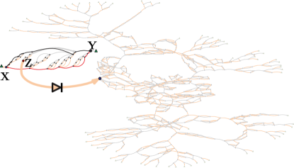
Figure 4: One-way “rabbit-hole” transitions. The transition out of the mesostate $Z$ inside the $\gamma_{\rm max}=0.05$ limit-cycle leads to a set of states, from which there does not appear to be a path back.

The transition from $W$ to $Y^{\prime}$ is RPM-violating, since it takes a short-cut by going directly to $Y^{\prime}$ without having $R$ as an intermediate mesostate. It turns out that the transition to $Y^{\prime}$ via $R\to A^{\prime}\to Y^{\prime}$ involve the soft-spot labeled as $5$, see Fig 2(a), and another two soft-spots. However, the alternative route $R\to V\to W\to Y^{\prime}$ is found to change the state of soft-spot $5$ during transition $V\to W$ under increasing strain. $W$ cannot transit into $R$ under a subsequent strain increase, because soft-spot $5$ has already changed its state when $V\to W$.

The construction of a network of mesostates that captures exclusively the plastic events, provides a methodology that enables us to analyze in detail how memory is encoded in periodically sheared amorphous solids. We are thus able to explicitly address for the first time many questions about memory formation phenomena observed in these systems. In particular, we see that the system reaching a limit-cycle, is a result of the two-level nature of most plastic events and the property that in most cases, interactions modify the dynamics (and hence the network) in a manner that does not impair reversibility. As a result, a hierarchy of cycles and sub-cycles emerges.

At the same time, the transition network and its topology provide a bird’s eye view on the athermal and quasistatic dynamics of an amorphous solid subject to arbitrary strain protocols. We believe that the prospect of relating the network topology to the activation and deactivation dynamics of interacting two-level systems provides a promising direction for understanding the reversible and irreversible features of the dynamics of amorphous solids and for constructing models that capture it.

Author contributions.

MM and IR contributed equally to the research of this work. KD, MM, IR and SS analyzed the results and wrote the paper.

References

- Keim et al. (2019) N. C. Keim, J. D. Paulsen, Z. Zeravcic, S. Sastry, and S. R. Nagel, Rev. Mod. Phys. 91, 035002 (2019).
- Paulsen et al. (2014) J. D. Paulsen, N. C. Keim, and S. R. Nagel, Phys. Rev. Lett 113, 068301 (2014).
- Fiocco et al. (2014) D. Fiocco, G. Foffi, and S. Sastry, Phys. Rev. Lett. 112, 025702 (2014).
- Fiocco et al. (2015) D. Fiocco, G. Foffi, and S. Sastry, J. Phys. Cond. Mat. 27, 194130 (2015).
- Mungan and Witten (2019) M. Mungan and T. A. Witten, Phys. Rev. E 99, 052132 (2019).
- Corte et al. (2008) L. Corte, P. M. Chaikin, J. P. Gollub, and D. J. Pine, Nature Physics 4, 420 (2008).
- Keim and Nagel (2011) N. C. Keim and S. R. Nagel, Phys. Rev. Lett. 107, 010603 (2011).
- Keim et al. (2013) N. C. Keim, J. D. Paulsen, and S. R. Nagel, Phys. Rev. E 88, 032306 (2013).
- Regev et al. (2013) I. Regev, T. Lookman, and C. Reichhardt, Phys. Rev. E 88, 062401 (2013).
- Fiocco et al. (2013) D. Fiocco, G. Foffi, and S. Sastry, Phys. Rev. E 88, 020301 (2013).
- Keim and Arratia (2014) N. C. Keim and P. E. Arratia, Phys. Rev. Lett. 112, 028302 (2014).
- Regev et al. (2015) I. Regev, J. Weber, C. Reichhardt, K. A. Dahmen, and T. Lookman, Nature communications 6, 8805 (2015).
- Hima Nagamanasa et al. (2014) K. Hima Nagamanasa, S. Gokhale, A. K. Sood, and R. Ganapathy, Phys. Rev. E 89, 062308 (2014).
- Kawasaki and Berthier (2016) T. Kawasaki and L. Berthier, Phys. Rev. E 94, 022615 (2016).
- Leishangthem et al. (2017) P. Leishangthem, A. D. Parmar, and S. Sastry, Nature communications 8, 14653 (2017).
- Adhikari and Sastry (2018) M. Adhikari and S. Sastry, The European Physical Journal E 41, 105 (2018).
- Keim et al. (2018) N. C. Keim, J. Hass, B. Kroger, and D. Wieker, arXiv preprint arXiv:1809.08505 (2018).
- Regev and Lookman (2019) I. Regev and T. Lookman, Journal of Physics: Condensed Matter 31, 045101 (2019).
- Bandi et al. (2018) M. Bandi, H. G. E. Hentschel, I. Procaccia, S. Roy, and J. Zylberg, EPL (Europhysics Letters) 122, 38003 (2018).
- Libál et al. (2012) A. Libál, C. Reichhardt, and C. J. Olson Reichhardt, Phys. Rev. E 86, 021406 (2012).
- Preisach (1935) F. Preisach, Z. Physik 94, 277 (1935).
- Middleton (1992) A. A. Middleton, Phys. Rev. Lett. 68, 670 (1992).
- Sethna et al. (1993) J. P. Sethna, K. Dahmen, S. Kartha, J. A. Krumhansl, B. W. Roberts, and J. D. Shore, Phys. Rev. Lett. 70, 3347 (1993).
- Argon (1979) A. Argon, Acta metallurgica 27, 47 (1979).
- Falk and Langer (1998) M. L. Falk and J. S. Langer, Phys. Rev. E 57, 7192 (1998).
- Manning and Liu (2011) M. L. Manning and A. J. Liu, Phys. Rev. Lett. 107, 108302 (2011).
- Eshelby (1957) J. D. Eshelby, Proc. R. Soc. Lond. A 241, 376 (1957).
- Maloney and Lemaître (2006) C. E. Maloney and A. Lemaître, Phys. Rev. E 74, 016118 (2006).
- Mungan and Terzi (2019) M. Mungan and M. M. Terzi, Ann. Henri Poincaré 20, 2819 (2019).
- Lerner and Procaccia (2009) E. Lerner and I. Procaccia, Phys. Rev. E 79, 066109 (2009).
- Note (1) Numerical implementation details are given in Supplement Section S1.1.
- Note (2) See Supplement Section S2.1 for a blown-up version of Fig. 1(b) along with a comparison of the transition graph obtained from a system with a larger number of particles.
- Regev et al. (2018) I. Regev, S. Sastry, K. Dahmen, and M. Mungan, (2018), in preparation.
- Note (3) We use green triangles to mark transitions to states not of interest, such as those beyond the catalog limit. See Supplement Section S1 for further details on the numerical procedure used for mesostate extraction, identification and transition graph construction.
- Stein and Newman (1995) D. L. Stein and C. M. Newman, Phys. Rev. E 51, 5228 (1995).