Image Deformation Meta-Networks for One-Shot Learning

Abstract

Humans can robustly learn novel visual concepts even when images undergo various deformations and lose certain information. Mimicking the same behavior and synthesizing deformed instances of new concepts may help visual recognition systems perform better one-shot learning, i.e., learning concepts from one or few examples. Our key insight is that, while the deformed images may not be visually realistic, they still maintain critical semantic information and contribute significantly to formulating classifier decision boundaries. Inspired by the recent progress of meta-learning, we combine a meta-learner with an image deformation sub-network that produces additional training examples, and optimize both models in an end-to-end manner. The deformation sub-network learns to deform images by fusing a pair of images — a probe image that keeps the visual content and a gallery image that diversifies the deformations. We demonstrate results on the widely used one-shot learning benchmarks (miniImageNet and ImageNet 1K Challenge datasets), which significantly outperform state-of-the-art approaches. Code is available at https://github.com/tankche1/IDeMe-Net.

(a)         (b)         (c)        (d)         (e) Figure 1: Illustration of a variety of image deformations: ghosted (a, b), stitched (c), montaged (d), and partially occluded (e) images.

1 Introduction

Deep architectures have made significant progress in various visual recognition tasks, such as image classification and object detection. This success typically relies on supervised learning from large amounts of labeled examples. In real-world scenarios, however, one may not have enough resources to collect large training sets or need to deal with rare visual concepts. It is also unlike the human visual system, which can learn a novel concept with very little supervision. One-shot or low/few-shot learning [4], which aims to build a classifier for a new concept from one or very few labeled examples, has thus attracted more and more attention.

Recent efforts to address this problem have leveraged a learning-to-learn or meta-learning paradigm  [25, 20, 28, 32, 31, 22, 33, 17, 5, 13]. Meta-learning algorithms train a learner, which is a parameterized function that maps labeled training sets to classifiers. Meta-learners are trained by sampling a collection of one-shot learning tasks and the corresponding datasets from a large universe of labeled examples of known (base) categories, feeding the sampled small training set to the learner to obtain a classifier, and then computing the loss of the classifier on the sampled test set. The goal is that the learner is able to tackle the recognition of unseen (novel) categories from few training examples.

Despite their noticeable performance improvements, these generic meta-learning algorithms typically treat images as black boxes and ignore the structure of the visual world. By contrast, our biological vision system is very robust and trustable in understanding images that undergo various deformations [27]. For instance, we can easily recognize the objects in Figure Image Deformation Meta-Networks for One-Shot Learning, despite ghosting (Figure Image Deformation Meta-Networks for One-Shot Learning(a, b)), stitching (Figure Image Deformation Meta-Networks for One-Shot Learning(c)), montaging (Figure Image Deformation Meta-Networks for One-Shot Learning(d)), and partially occluding (Figure Image Deformation Meta-Networks for One-Shot Learning(e)) the images. While these deformed images may not be visually realistic, our key insight is that they still maintain critical semantic information and presumably serve as “hard examples” that contribute significantly to formulating classifier decision boundaries. Hence, by leveraging such modes of deformations shared across categories, the synthesized deformed images could be used as additional training data to build better classifiers.

A natural question then arises: how could we produce informative deformations? We propose a simple parametrization that linearly combines a pair of images to generate the deformed image. We use a probe image to keep the visual content and overlay a gallery image on a patch level to introduce appearance variations, which could be attributed to semantic diversity, artifacts, or even random noise. Figure 5 shows some examples of our deformed images. Importantly, inspired by [30], we learn to deform images that are useful for a classification objective by end-to-end meta-optimization that includes image deformations in the model.

Our Image Deformation Meta-Network (IDeMe-Net) thus consists of two components: a deformation sub-network and an embedding sub-network. The deformation sub-network learns to generate the deformed images by linearly fusing the patches of probe and gallery images. Specifically, we treat the given small training set as the probe images and sample additional images from the base categories to form the gallery images. We evenly divide the probe and gallery images into nine patches, and the deformation sub-network estimates the combination weight of each patch. The synthesized images are used to augment the probe images and train the embedding sub-network, which maps images to feature representations and performs one-shot classification. The entire network is trained in an end-to-end meta-learning manner on base categories.

Our contributions are three-fold. (1) We propose a novel image deformation framework based on meta-learning to address one-shot learning, which leverages the rich structure of shared modes of deformations in the visual world. (2) Our deformation network learns to synthesize diverse deformed images, which effectively exploits the complementarity and interaction between the probe and gallery image patches. (3) By using the deformation network, we effectively augment and diversify the one-shot training images, leading to a significant performance boost on one-shot learning tasks. Remarkably, our approach achieves state-of-the-art performance on both the challenging ImageNet1K and miniImageNet datasets.

2 Related Work

Meta-Learning. Typically, meta-learning [25, 24, 20, 28, 32, 31, 22, 33, 17, 5, 13, 36, 15] aims at training a parametrized mapping from a few training instances to model parameters in simulated one-shot learning scenarios. Other meta-learning strategies in one-shot learning include graph CNNs [7] and memory networks [19, 1]. Attention is also introduced in meta-learning, in ways of analyzing the relation between visual and semantic representations [29] and learning the combination of temporal convolutions and soft attention [14]. Different from prior work, we focus on exploiting the complementarity and interaction between visual patches through the meta-learning mechanism.

Metric Learning. This is another important line of work in one-shot learning. The goal is to learn a metric space which can be optimized for one-shot learning. Recent work includes Siamese networks [11], matching networks [28], prototypical networks [22], relation networks [23], and dynamic few-shot learning without forgetting [8].

Data Augmentation. The key limitation of one-shot learning is the lack of sufficient training images. As a common practice, data augmentation has been widely used to help train supervised classifiers [12, 2, 34]. The standard techniques include adding Gaussian noise, flipping, rotating, rescaling, transforming, and randomly cropping training images. However, the generated images in this way are particularly subject to visual similarity with the original images. In addition to adding noise or jittering, previous work seeks to augment training images by using semi-supervised techniques [31, 18, 16] and utilizing relation between visual and semantic representations [3] , or directly synthesizing new instances in the feature domain [9, 30, 21, 6] to transfer knowledge of data distribution from base classes to novel classes. By contrast, we also use samples from base classes to help synthesize deformed images but directly aim at maximizing the one-shot recognition accuracy.

The most relevant to our approach is the work of [30, 35]. Wang et al. [30] introduce a GAN-like generator to hallucinate novel instances in the feature domain by adding noise, whereas we focus on learning to deform two real images in the image domain without introducing noise. Zhang et al. [35] randomly sample image pairs and linearly combine them to generate additional training images. In this mixup augmentation, the combination is performed with weights randomly sampled from a prior distribution and is thus constrained to be convex. The label of the generated image is similarly the linear combination of the labels (as one-hot label vectors) of the image pairs. However, they ignore structural dependencies between images as well as image patches. By contrast, we learn classifiers to select images that are similar to the probe images from the unsupervised gallery image set. Our combination weights are learned through a deformation sub-network on the image patch level and the combination is not necessarily convex. In addition, our generated image preserves the label of its probe image. Comparing with these methods, our approach learns to dynamically fuse patches of two real images in an end-to-end manner. The produced images maintain the important patches of original images while being visually different from them, thus facilitating training one-shot classifiers.

3 One-Shot Learning Setup

Following recent work [28, 17, 5, 22, 30], we establish one-shot learning in a meta-learning framework: we have a base category set $\mathcal{C}_{base}$ and a novel category set $\mathcal{C}_{novel}$, in which $\mathcal{C}_{base}\cap\mathcal{C}_{novel}=\emptyset$; correspondingly, we have a base dataset $D_{base}=\left\{\left(\mathbf{I}_{i},y_{i}\right),y_{i}\in\mathcal{C}_{base}\right\}$ and a novel dataset $D_{novel}=\left\{\left(\mathbf{I}_{i},y_{i}\right),y_{i}\in\mathcal{C}_{novel}\right\}$. We aim to learn a classification algorithm on $D_{base}$ that can generalize to unseen classes $C_{novel}$ with one or few training examples per class.

To mimic the one-shot learning scenario, meta-learning algorithms learn from a collection of $N$-way-$m$-shot classification tasks/datasets sampled from $D_{base}$ and are evaluated in a similar way on $D_{novel}$. Each of these sampled datasets is termed as an episode, and we thus have different meta-sets for meta-training and meta-testing. Specifically, we randomly sample $N$ classes $L\sim C_{k}$ for a meta-training (i.e., $k=base$) or meta-testing episode (i.e., $k=novel$). We then randomly sample $m$ and $q$ labeled images per class in $L$ to construct the support set $S$ and query set $Q$, respectively, i.e., $|S|=N\times m$ and $|Q|=N\times q$. During meta-training, we sample $S$ and $Q$ to train our model. During meta-testing, we evaluate by averaging the classification accuracy on query sets $Q$ of many meta-testing episodes.

We view the support set as supervised probe images and different from the previous work, we introduce an additional gallery image set $G$ that serves as an unsupervised image pool to help generate deformed images. To construct $G$, we randomly sample some images per base class from the base dataset, i.e., $G\sim D_{base}$. The same $G$ is used in both the meta-training and meta-testing episodes. Note that since it is purely sampled from $D_{base}$, the newly introduced $G$ does not break the standard one-shot setup as in [22, 5, 17]. We do not introduce any additional images from the novel categories $\mathcal{C}_{novel}$.

4 Image Deformation Meta-Networks

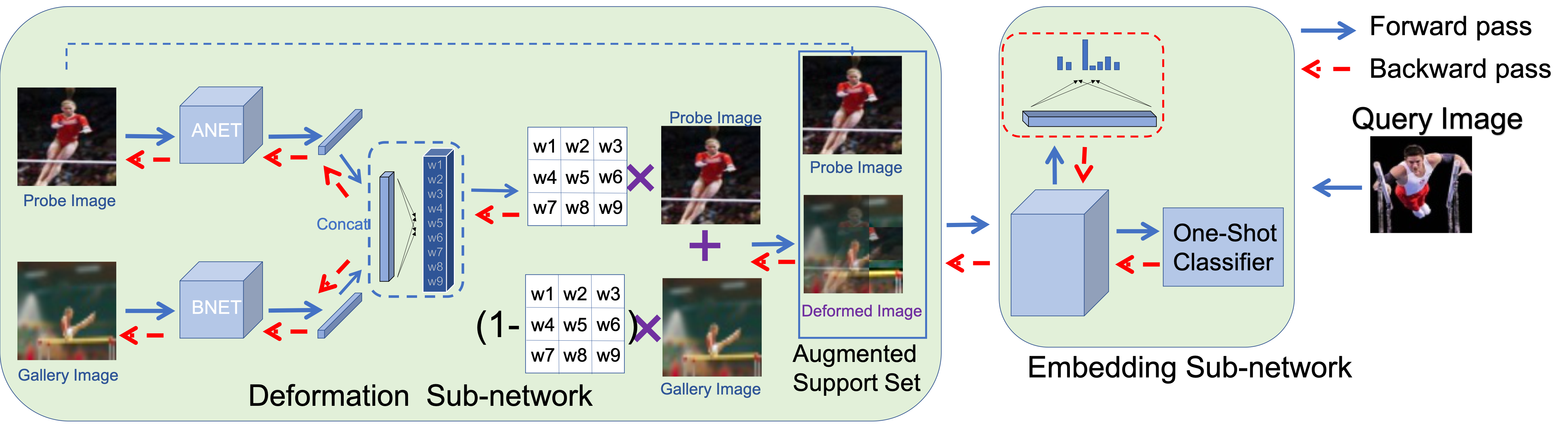
Figure 2: The overall architecture of our image deformation meta-network (IDeMe-Net).

We now explain our image deformation meta-network (IDeMe-Net) for one-shot learning. Figure 2 shows the architecture of IDeMe-Net $f_{\theta}(\cdot)$ parametrized by $\theta$. IDeMe-Net is composed of two modules — a deformation sub-network and an embedding sub-network. The deformation sub-network adaptively fuses the probe and gallery images to synthesize the deformed images. The embedding sub-network maps the images to feature representations and then constructs the one-shot classifier. The entire meta-network is trained in an end-to-end manner.

4.1 Deformation Sub-network

This sub-network $f_{\theta_{def}}\left(\cdot\right)$ learns to explore the interaction and complementarity between the probe images $\mathbf{I}_{probe}$ ($\left(\mathbf{I}_{probe},y_{probe}\right)\in S$) and the gallery images $\mathbf{I}_{gallery}\in G$, and fuses them to generate the synthesized deformed images $\mathbf{I}_{syn}$, i.e., $\mathbf{I}_{syn}=f_{\theta_{def}}\left(\mathbf{I}_{probe},\mathbf{I}_{gallery}\right)$. Our goal is to synthesize meaningful deformed images such that $y_{syn}=y_{probe}$. This is achieved by using two strategies: (1) $y_{syn}=y_{probe}$ is explicitly enforced as a constraint during the end-to-end optimization; (2) we propose an approach to sample $\mathbf{I}_{gallery}$ that are visually or semantically similar to the images of $y_{probe}$. Specifically, for each class $y_{probe}$, we directly use the feature extractor and one-shot classifier learned in the embedding sub-network to select the top $\epsilon\%$ images from $G$ which have the highest class probability of $y_{probe}$. From this initial pool of images, we randomly sample $\mathbf{I}_{gallery}$ for each probe image $\left(\mathbf{I}_{probe},y_{probe}\right)$. Note that during meta-training, both $\mathbf{I}_{probe}$ and $\mathbf{I}_{gallery}$ are randomly sampled from base classes, so they might belong to the same class. We find that further constraining them to belong to different base classes has little impact on the performance. During meta-testing, $\mathbf{I}_{probe}$ and $\mathbf{I}_{gallery}$ belong to different classes, with $\mathbf{I}_{probe}$ sampled from novel classes and $\mathbf{I}_{gallery}$ still from base classes.

Two branches, ANET and BNET, are used to parse $\mathbf{I}_{probe}$ and $\mathbf{I}_{gallery}$, respectively. Each of them is a residual network [10] without fully-connected layers. The outputs of ANET and BNET are then concatenated to be fed into a fully-connected layer, which produces a 9-D weight vector $w$. As shown in Figure 2, we evenly divide the images into $3\times 3$ patches. The deformed image is thus simply generated as a linearly weighted combination of $\mathbf{I}_{probe}$ and $\mathbf{I}_{gallery}$ on the patch level. That is, for the $q$th patch, we have

$$\mathbf{I}_{syn,q}=w_{q}\mathbf{I}_{probe,q}+\left(1-w_{q}\right)\mathbf{I}_{gallery,q}.$$ (1)

We assign the class label $y_{probe}$ to the synthesized deformed image $\mathbf{I}_{syn}$. For any probe image $\mathbf{I}_{probe}^{i}$, we sample $n_{aug}$ gallery images from the corresponding pool and produce $n_{aug}$ synthesized deformed images. We thus obtain an augmented support set

$$\tilde{S}=\left\{\left(\mathbf{I}^{i}_{probe},y^{i}_{probe}\right),\left\{\left(\mathbf{I}_{syn}^{i,j},y_{probe}^{i,j}\right)\right\}_{j=1}^{n_{aug}}\right\}_{i=1}^{N\times m}.$$ (2)

4.2 Embedding Sub-network

The embedding sub-network $f_{\theta_{emb}}(\cdot)$ consists of a deep convolutional network for feature extraction and a non-parametric one-shot classifier. Given an input image $\mathbf{I}$, we use a residual network [10] to produce its feature representation $f_{\theta_{emb}}\left(\mathbf{I}\right)$. To facilitate the training process, we introduce an additional softmax classifier, i.e., a fully-connected layer on top of the embedding sub-network with a cross-entropy loss (CELoss), that outputs $|\mathcal{C}_{base}|$ scores.

4.3 One-Shot Classifier

Due to its superior performance, we use the non-parametric prototype classifier [22] as the one-shot classifier. During each episode, given the sampled $S$, $Q$, and $G$, the deformation sub-network produces the augmented support set $\tilde{S}$. Following [22], we calculate the prototype vector $p_{\theta}^{c}$ for each class $c$ in $\tilde{S}$ as

$$p_{\theta}^{c}=\frac{1}{Z}\sum_{(\mathbf{I}_{i},y_{i})\in\tilde{S}}f_{\theta_{emb}}\left(\mathbf{I}_{i}\right)\cdot\left\llbracket y_{i}=c\right\rrbracket,$$ (3)

where $Z=\Sigma_{(\mathbf{I}_{i},y_{i})\in\tilde{S}}\left\llbracket y_{i}=c\right\rrbracket$ is the normalization factor. $\left\llbracket\cdot\right\rrbracket$ is the Iverson’s bracket notation: $\left\llbracket x\right\rrbracket=1$ if $x$ is true, and $0$ otherwise. Given any query image $\mathbf{I}_{i}\in Q$, its probability of belonging to class $c$ is computed as

$$P_{\theta}\left(y_{i}=c\text{$\mid$}\mathbf{I}_{i}\right)=\frac{\mathrm{exp}\left(-\left\|\mathit{f}_{\theta_{emb}}\left(\mathbf{I}_{i}\right)-\mathit{p}_{\theta}^{c}\right\|^{2}\right)}{\sum_{j=1}^{N}\mathrm{exp}\left(-\left\|f_{\theta_{emb}}\left(\mathbf{I}_{i}\right)-p_{\theta}^{j}\right\|^{2}\right)},$$ (4)

where $\parallel\cdot\parallel$ indicates the Euclidean distance. The one-shot classifier $P$ thus predicts the class label of $\mathbf{I}_{i}$ as the highest probability over $N$ classes.

5 Training Strategy of IDeMe-Net

Algorithm 1 Meta-training procedure of our IDeMe-Net $f_{\theta}$. $G$ is the fixed gallery constructed from $\mathcal{C}_{base}$.

1:procedure Meta-Train_Episode

2:The procedure of one meta-training episode

3:     $L\leftarrow$ randomly sample $N$ classes from $\mathcal{C}_{base}$

4:     $S\leftarrow$ randomly sample instances belonging to $L$

5:     //sample the support set

6:     $Q\leftarrow$ randomly sample instances belonging to $L$

7:     //sample the query set

8:     train the prototype classifier $P$ from $f_{\theta_{emb}}(S)$

9:     $\tilde{S}\leftarrow S$ $\triangleright$ initialize the augment support set

10:     for $c$ in $L$ do$\triangleright$ enumerate the chosen classes

11:         $pool\leftarrow$use $P$ to select $\epsilon\%$ images in $G$ that have the highest class probability of $c$

12:         for $(\mathbf{I}_{probe},c)$ in $S_{c}$ do

13:              for $j=1$ to $n_{aug}$ do

14:                  $\mathbf{I}_{gallery}\leftarrow$ randomly sample instances from $pool$

15:                  $\mathbf{I}_{syn}\leftarrow f_{\theta_{def}}(\mathbf{I}_{probe},\mathbf{I}_{gallery})$

16:                  $\tilde{S}\leftarrow\tilde{S}\cup(\mathbf{I}_{syn},c)$

17:              end for

18:         end for

19:     end for

20:     train the prototype classifier $\tilde{P}$ from $f_{\theta_{emb}}(\tilde{S})$

21:     use $\tilde{P}$ to classify $f_{\theta_{emb}}(Q)$ and obtain the prototype loss

22:     use the softmax classifier to classify $f_{\theta_{emb}}(\tilde{S})$ and obtain the CELoss

23:     update $\theta_{emb}$ with the CELoss

24:     update $\theta_{def}$ with the prototype loss

25:end procedure

5.1 Training Loss

Training the entire IDeMe-Net includes two subtasks: (1) training the deformation sub-network which maximally improves the one-shot classification accuracy; (2) building the robust embedding sub-network which effectively deals with various synthesized deformed images. Note that our one-shot classifier has no parameters, which does not need to be trained. We use the prototype loss and the cross-entropy loss to train these two sub-networks, respectively.

Update the deformation sub-network. We optimize the following prototype loss function to endow the deformation sub-network with the desired one-shot classification ability:

$$\mathrm{min}_{\theta}\mathbb{E}_{G,L\sim D_{base}}\mathbb{E}_{S,Q\sim L}\left[\sum_{\left(\mathbf{I}_{i},y_{i}\right)\in Q}-\mathrm{log}P_{\theta}\left(y_{i}\mid\mathbf{I}_{i}\right)\right],$$ (5)

where $P_{\theta}\left(y_{i}\mid\mathbf{I}_{i}\right)$ is the one-shot classifier in Eq. (4). Using the prototype loss encourages the deformation sub-network to generate diverse instances to augment the support set.

Update the embedding sub-network. We use the cross-entropy loss to train the embedding sub-network to directly classify the augmented support set $\tilde{S}$. Note that with the augmented support set $\tilde{S}$, we have relatively more training instances to train this sub-network and the cross-entropy loss is the standard loss function in training a supervised classification network. Empirically, we find that using the cross-entropy loss speeds up the convergence and improves the recognition performance than using the prototype loss only.

5.2 Training Strategy

We summarize the entire training procedure of our IDeMe-Net on the base dataset $D_{base}$ in Algorithm 1. We have access to the same, predefined gallery $G$ from $D_{base}$ for both meta-training and meta-testing. During meta-training, we sample the $N$-way-$m$-shot training episode to produce $S$ and $Q$ from $D_{base}$. The embedding sub-network learns an initial one-shot classifier on $S$ using Eq. (4). Given a probe image $\mathbf{I}_{probe}$, we then sample the gallery images $\mathbf{I}_{gallery}\sim G$ and train the deformation sub-network to generate the augmented support set $\tilde{S}$ using Eq. (1). $\tilde{S}$ is further used to update the embedding sub-network and learn a better one-shot classifier. We then conduct the final one-shot classification on the query set $Q$ and back-propagate the prediction error to update the entire network. During meta-testing, we sample the $N$-way-$m$-shot testing episode to produce $S$ and $Q$ from the novel dataset $D_{novel}$.

6 Experiments

	Method	$m=1$	$2$	$5$	$10$	$20$
Baselines	Softmax	– / 16.3	– / 35.9	– / 57.4	– / 67.3	– / 72.1
	LR	18.3/42.8	26.0/54.7	35.8/66.1	41.1/71.3	44.9/74.8
	SVM	15.9/36.6	22.7/48.4	31.5/61.2	37.9/69.2	43.9/74.6
	Prototype Classifier	17.1/39.2	24.3/51.1	33.8/63.9	38.4/69.9	44.1/74.7
Competitors	Matching Network [28]	– / 43.0	– / 54.1	– / 64.4	– / 68.5	– / 72.8
	Prototypical Network [22]	16.9/41.7	24.0/53.6	33.5/63.7	37.7/68.2	42.7/72.3
	Generation SGM [9]	– / 34.3	– / 48.9	– / 64.1	– / 70.5	– / 74.6
	PMN [30]	– / 43.3	– / 55.7	– / 68.4	– / 74.0	– / 77.0
	PMN w/ H [30]	– / 45.8	– / 57.8	– / 69.0	– / 74.3	– / 77.4
	Cos & Att. [8]	– / 46.0	– / 57.5	– / 69.1	– / 74.8	– / 78.1
	CP-AAN [6]	– / 48.4	– / 59.3	– / 70.2	– / 76.5	– / 79.3
Augmentation	Flipping	17.4/39.6	24.7/51.2	33.7/64.1	38.7/70.2	44.2/74.5
	Gaussian Noise	16.8/39.0	24.0/51.2	33.9/63.7	38.0/69.7	43.8/74.5
	Gaussian Noise (feature level)	16.7/39.1	24.2/51.4	33.4/63.3	38.2/69.5	44.0/74.2
	Mixup [35]	15.8/38.7	24.6/51.4	32.0/61.1	38.5/69.2	42.1/72.9
Ours	IDeMe-Net	23.1/51.0	30.1/60.9	39.3/70.4	42.7/73.4	45.0/75.1

Table 1: Top-1 / Top-5 accuracy (%) on novel classes of the ImageNet 1K Challenge dataset. We use ResNet-10 as the embedding sub-network. $m$ indicates the number of training examples per class. Our IDeMe-Net consistently achieves the best performance.

Our IDeMe-Net is evaluated on two standard benchmarks: miniImageNet [28] and ImageNet 1K Challenge [9] datasets. miniImageNet is a widely used benchmark in one-shot learning, which includes 600 images per class and has 100 classes in total. Following the data split in [17], we use 64, 16, 20 classes as the base, validation, and novel category set, respectively. The hyper-parameters are cross-validated on the validation set. Consistent with [28, 17], we evaluate our model in 5-way-5-shot and 5-way-1-shot settings.

For the large-scale ImageNet 1K dataset, we divide the original 1K categories into 389 base ($D_{base}$) and 611 novel ($D_{novel}$) classes following the data split in [9]. The base classes are further divided into two disjoint subsets: base validation set $D_{base}^{cv}$ (193 classes) and evaluation set $D_{base}^{fin}$ (196 classes) and the novel classes are divided into two subsets as well: novel validation set $D_{novel}^{cv}$ (300 classes) and evaluation set $D_{novel}^{fin}$ (311 classes). We use the base/novel validation set $D^{cv}$ for cross-validating hyper-parameters and use the base/novel evaluation set $D^{fin}$ to conduct the final experiments. The same experimental setup is used in [9] and the reported results are averaged over 5 trials. Here we focus on synthesizing novel instances and we thus evaluate the performance primarily on novel classes, i.e., 311-way-$m$-shot settings, which is also consistent with most of the contemporary work [28, 22, 17].

Method $m=1$ $2$ $5$ $10$ Softmax – / 28.2 – / 51.0 – / 71.0 – / 78.4 SVM 20.1/41.6 29.4/57.7 42.6/72.8 49.9/79.1 LR 22.9/47.9 32.3/61.3 44.3/73.6 50.9/78.8 Proto-Clsf 20.8/43.1 29.9/58.1 42.4/72.3 49.5/79.0 G-SGM [9] – / 47.3 – / 60.9 – / 73.7 – / 79.5 PMN [30] – / 53.3 – / 65.2 – / 75.9 – / 80.1 PMN w/ H [30] – / 54.7 – / 66.8 – / 77.4 – / 81.4 IDeMe-Net (Ours) 30.3/60.1 39.7/69.6 47.5/77.4 51.3/80.2

Table 2: Top-1 / Top-5 accuracy (%) on novel classes of the Imagenet 1K Challenge dataset. We use ResNet-50 as the embedding sub-network. $m$ indicates the number of training examples per class. Proto-Clsf and G-SGM denote the prototype classifier and generation SGM [9], respectively.

6.1 Results on ImageNet 1K Challenge

Setup. We use ResNet-10 architectures for ANET and BNET (i.e., the deformation sub-network). For a fair comparison with [9, 30], we evaluate the performance of using ResNet-10 (Table 1) and ResNet-50 (Table 2) for the embedding sub-network. Stochastic gradient descent (SGD) is used to train IDeMe-Net in an end-to-end manner. It gets converged over 100 epochs. The initial learning rates of ANET, BNET, and the embedding sub-network are set as $3\times 10^{-3}$, $3\times 10^{-3}$, and $10^{-1}$, respectively, and decreased by $1/10$ every 30 epochs. The batch size is set as 32. We randomly sample 10 images per base category to construct the gallery $G$ and we set $\epsilon$ as 2. Note that $G$ is fixed during the entire experiments. ANET, BNET, and the embedding sub-network are trained from scratch on $D_{base}$. Our model is evaluated on $D_{novel}$. $n_{aug}$ is cross-validated as 8, which balances between the computational cost and the augmented training data scale. In practice, we perform stage-wise training to overcome potential negative influence caused by misleading training images synthesized by the initial deformation sub-network. Specifically, to make the training more robust, we first fix the deformation sub-network and train the embedding sub-network with real and deformed images. Here the deformed images are synthesized by linearly combining two images on a patch level with a randomly sampled weight vector $w$. Note that these two images are sampled from the same category. Then we fix the embedding sub-network and learn the deformation sub-network to reduce the discrepancy between synthesized and real images. Finally, we train the embedding and deformation sub-networks jointly (i.e., the entire IDeMe-Net) to allow them to cooperate with each other.

Baselines and Competitors. We compare against several baselines and competitors as follows. (1) We directly train a ResNet-10 feature extractor on $D_{base}$ and use it to compute features on $D_{novel}$. We then train standard supervised classifiers on $D_{novel}$, including neural network, support vector machine (SVM), logistic regression (LR), and prototype classifiers. The neural network classifier consists of a fully-connected layer and a softmax layer. (2) We compare with state-of-the-art approaches to one-shot learning, such as matching networks [28], generation SGM [9], prototypical networks [22], Cosine Classifier & Att. Weight Gen (Cos & Att.) [8], CP-ANN [6], PMN, and PMN w/ H [30]. (3) The data augmentation methods are also compared — flipping: the input image is flipped from left to right; Gaussian noise: cross-validated Gaussian noise $\mathcal{N}\left(0,10\right)$ is added to each pixel of the input image; Gaussian noise (feature level): cross-validated Gaussian noise $\mathcal{N}\left(0,0.3\right)$ is added to each dimension of the ResNet feature for each image; Mixup: using mixup [35] to combine probe and gallery images. For fair comparisons, all these augmentation methods use the prototype classifier as the one-shot classifier.

	Method	$m=1$	$2$	$5$	$10$	$20$
Baselines	LR	18.3/42.8	26.0/54.7	35.8/66.1	41.1/71.3	44.9/74.8
	Prototype Classifier	17.1/39.2	24.3/51.1	33.8/63.9	38.4/69.9	44.1/74.7
Variants	IDeMe-Net - CELoss	21.3/50.0	28.0/58.3	37.7/69.4	41.3/71.6	44.3/74.3
	IDeMe-Net - Proto Loss	15.3/36.7	21.4/50.4	31.7/62.0	37.9/69.0	43.7/73.7
	IDeMe-Net - Predict	17.0/39.3	24.0/50.7	33.6/63.5	38.0/69.2	43.7/73.8
	IDeMe-Net - Aug. Testing	17.0/39.1	24.30/51.3	33.5/63.8	38.0/69.1	43.8/74.5
	IDeMe-Net - Def. Network	15.9/38.0	24.1/50.1	32.6/63.3	38.2/68.9	42.4/73.1
	IDeMe-Net - Gallery	17.5/39.4	24.2/51.4	33.5/63.7	38.7/70.3	44.4/74.5
	IDeMe-Net - Deform	15.7/37.8	22.7/49.8	31.9/62.6	38.0/68.7	43.5/73.8
Patch Size	IDeMe-Net ($1\times 1$)	16.2/39.3	24.4/52.1	32.9/63.0	38.8/69.5	42.7/73.2
	IDeMe-Net ($5\times 5$)	24.1/51.7	30.3/61.2	39.6/70.4	42.4/73.2	44.3/74.6
	IDeMe-Net ($7\times 7$)	23.8/52.1	30.2/61.3	39.1/70.2	42.7/73.1	44.5/74.7
	IDeMe-Net (pixel level)	17.3/39.0	23.8/51.2	34.1/63.7	38.5/70.2	43.9/74.5
Ours	IDeMe-Net	23.1/51.0	30.4/60.9	39.3/70.4	42.7/73.4	45.0/75.1

Table 3: Top-1 / Top-5 accuracy (%) of the ablation study on novel classes of the ImageNet 1K Challenge dataset. We use ResNet-10 as the embedding sub-network. $m$ indicates the number of training examples per class. Our full model achieves the best performance.

Results. Tables 1 and 2 summarize the results of using ResNet-10 and ResNet-50 as the embedding sub-network, respectively. For example, using ResNet-10, the top-5 accuracy of IDeMe-Net in Table 1 is superior to the prototypical network by 7% when $m=1,2,5$, showing the sample efficiency of IDeMe-Net for one-shot learning. With more data (e.g., $m=10,20$), while the plain prototype classifier baseline performs worse than other baselines (e.g., PMN), our deformed images coupled with the prototype classifier still have significant effect (e.g., $3.5$ point boost when $m=10$). The top-1 accuracy demonstrates the similar trend. Using ResNet-50 as the embedding sub-network, the performance of all the approaches improves and our IDeMe-Net consistently achieves the best performance, as shown in Table 2. Figure 3(a) further highlights that our IDeMe-Net consistently outperforms all the baselines by large margins.

6.2 Ablation Study on ImageNet 1K Challenge

We conduct extensive ablation studies to evaluate the contribution of each component in our model.

Variants of IDeMe-Net. We consider seven different variants of our IDeMe-Net, as shown in Figure 3(b) and Table 3. (1) ‘IDeMe-Net - CELoss’: the IDeMe-Net is trained using only the prototype loss without the cross-entropy loss (CELoss). (2) ‘IDeMe-Net - Proto Loss’: the IdeMe-Net is trained using only the cross-entropy loss without the prototype loss. (3) ‘IDeMe-Net - Predict’: the gallery images are randomly chosen in IDeMe-Net without predicting their class probability. (4) ‘IDeMe-Net - Aug. Testing’: the deformed images are not produced in the meta-testing phase. (5) ‘IDeMe-Net - Def. Network’: the combination weights in Eq. (1) are randomly generated instead of using the learned deformation sub-network. (6) ‘IDeMe-Net - Gallery’: the gallery images are directly sampled from the support set instead of constructing an additional Gallery. (7) ‘IDeMe-Net - Deform’: we simply use the gallery images to serve as the deformed images. As shown in Figure 3(b), our full IDeMe-Net model outperforms all these variants, showing that each component is essential and complementary to each other.

We note that (1) Using CELoss and prototype loss to update the embedding and deformation sub-networks, respectively, achieves the best result. As shown in Figure 3(b), the accuracy of ‘IDeMe-Net - CELoss’ is marginally lower than IDeMe-Net but still higher than the prototype classifier baseline, while ‘IDeMe-Net - Proto Loss’ underperforms the baseline. (2) Our strategy for selecting the gallery images is the key to diversify the deformed images. Randomly choosing the gallery images (‘IDeMe-Net - Predict’) or sampling the gallery images from the support set (‘IDeMe-Net - Gallery’) obtains no performance improvement. One potential explanation is that they only introduce noise or redundancy and do not bring in useful information. (3) Our improved performance mainly comes from the diversified deformed images, rather than the embedding sub-network. Without producing the deformed images in the meta-testing phase (‘IDeMe-Net - Aug. Testing’), the performance is close to the baseline, suggesting that training on the deformed images does not obviously benefit from the embedding sub-network. (4) Our meta-learned deformation sub-network effectively exploits the complementarity and interaction between the probe and gallery image patches, producing the key information in the deformed images. To show this point, we investigate two deformation strategies: randomly generating the weight vector $w$ (‘IDeMe-Net - Def. Network’) and setting all the weights to be 0 (‘IDeMe-Net - Deform’); in the latter case, it is equivalent to purely using the gallery images to serve as the deformed images. Both strategies perform worse than the prototype classifier baseline, indicating the importance of meta-learning a deformation strategy.

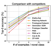
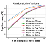
(a)	(b)
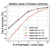
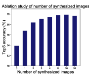
(c)	(d)

Figure 3: Ablation study on ImageNet 1K Challenge dataset: (a) highlights the comparison with several competitors; (b) shows the impact of different components on our IDeMe-Net; (c) analyzes the impact of different division schemes; (d) shows how the performance changes with respect to the number of synthesized deformed images. Best viewed in color with zoom.

Different division schemes. In the deformation sub-network and Eq. (1), we evenly split the image into $3\times 3$ patches. Some alternative division schemes are compared in Table 3 and Figure 3(c). Specifically, we consider the $1\times 1$, $5\times 5$, $7\times 7$, and pixel-level division schemes and report the results as IDeMe-Net ($1\times 1$), IDeMe-Net ($5\times 5$), IDeMe-Net ($7\times 7$), and IDeMe-Net (pixel level), respectively. The experimental results suggest the patch-level fusion, rather than image-level or pixel-level fusion in our IDeMe-Net. The image-level division ($1\times 1$) ignores the local image structures and deforms through a global combination, thus decreasing the diversity. The pixel-level division is particularly subject to the disarray of the local information, while the patch-level division ($3\times 3$, $5\times 5$, and $7\times 7$) considers image patches as the basic unit to maintain some local information. In addition, the results show that using a fine-grained patch size (e.g., $5\times 5$ division and $7\times 7$ division) may achieve slightly better results than our $3\times 3$ division. In brief, our patch-level division not only maintains the critical region information but also increases diversity.

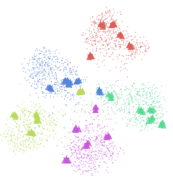
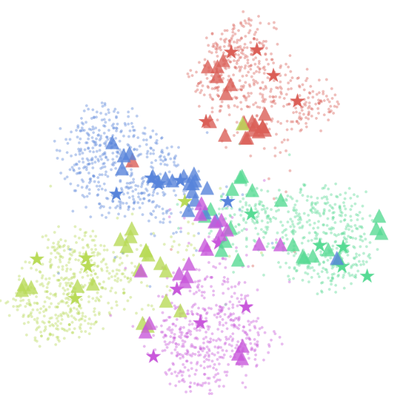
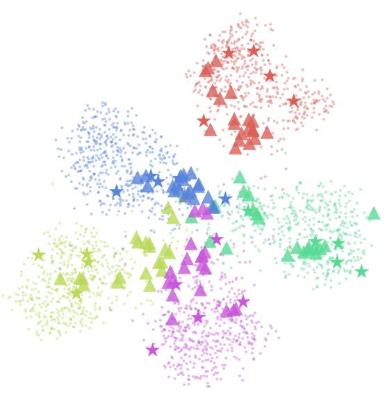
(a) Gaussian Baseline	(b) IDeMe-Net - Deform	(c) IDeMe-Net

Figure 4: t-SNE visualization of 5 novel classes. Dots, stars, and triangles represent the real examples, the probe images, and the synthesized deformed images, respectively. (a) Synthesis by adding Gaussian noise. (b) Synthesis by directly using the gallery images. (c) Synthesis by our IDeMe-Net. Best viewed in color with zoom.

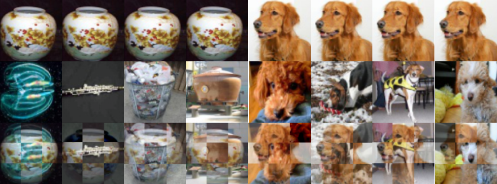
Figure 5: Examples of the deformed images during meta-testing. 1st row: probe images of novel classes. 2nd: gallery images of base classes. 3rd: synthesized images. The probe-gallery image pairs from left to right: vase–jellyfish, vase–oboe, vase–garbage bin, vase–soup pot, golden retriever–poodle, golden retriever–walker hound, golden retriever–walker hound, and golden retriever–poodle. Best viewed in color with zoom.

Number of synthesized deformed images. We also show how the top-5 accuracy changes with respect to the number of synthesized deformed images in Figure 3(d). Specifically, we change the number of synthesized deformed images $n_{aug}$ in the deformation sub-network, and plot the 5-shot top-5 accuracy on the Imagenet 1K Challenge dataset. It shows that when $n_{aug}$ is changed from $0$ to 8, the performance of our IDeMe-Net is gradually improved. The performance saturates when enough deformed images are generated ($n_{aug}>8$).

Visualization of deformed images in feature space. Figure 4 shows the t-SNE [26] visualization of 5 novel classes from our IDeMe-Net, the Gaussian noise baseline, and the ‘IDeMe-Net - Deform’ variant. For the Gaussian noise baseline, the synthesized images are heavily clustered and close to the probe images. By contrast, the synthesized deformed images of our IDeMe-Net scatter widely in the class manifold and tend to locate more around the class boundaries. For ‘IDeMe-Net - Deform’, the synthesized images are the same as the gallery images and occasionally fall into manifolds of other classes. Interesting, comparing Figure 4(b) and Figure 4(c), our IDeMe-Net effectively deforms those misleading gallery images back to the correct class manifold.

Visualization of deformed images in image space. Here we show some examples of our deformed images on novel classes in Figure 5. We can observe that the deformed images (in the third row) are visually different from the probe images (in the first row) and the gallery images (in the second row). For novel classes (e.g., vase and golden retriever), our method learns to find visual samples that are similar in shape and geometry (e.g., jelly fish, garbage bin, and soup pot) or similar in appearance (e.g., poodle and walker hound). By doing so, the deformed images preserve important visual content from the probe images and introduce new visual contents from the gallery images, thus diversifying and augmenting the training images in a way that maximizes the one-shot classification accuracy.

6.3 Results on miniImageNet

Method	miniImageNet ($\%$)
	1-shot	5-shot
MAML [5]	48.70±1.84	63.11±0.92
Meta-SGD [13]	50.47±1.87	64.03±0.94
Matching Network [28]	43.56±0.84	55.31±0.73
Prototypical Network [22]	49.42±0.78	68.20±0.66
Relation Network [23]	57.02±0.92	71.07±0.69
SNAIL [14]	55.71±0.99	68.88±0.92
Delta-Encoder [21]	58.7	73.6
Cos & Att. [8]	55.45±0.89	70.13 ±0.68
Prototype Classifier	52.54±0.81	72.71±0.73
IDeMe-Net (Ours)	59.14±0.86	74.63±0.74

Table 4: Top-1 accuracy (%) on novel classes of the miniImageNet dataset. “±” indicates $95\%$ confidence intervals over tasks.

Setup and Competitors. We use a ResNet-18 architecture as the embedding sub-network. We randomly sample 30 images per base category to construct the gallery $G$. Other settings are the same as those on the ImageNet 1k Challenge dataset. As summarized in Table 4, we mainly focus on three groups of competitors: (1) meta-learning algorithms, such as MAML [5] and Meta-SGD [13]; (2) metric learning algorithms, including matching networks [28], prototypical networks [22], relation networks [23], SNAIL [14], delta-encoder [21], and Cosine Classifier & Att. Weight Gen (Cos & Att.) [8].

Results. We report the results in Table 4. Impressively, our IDeMe-Net consistently outperforms all these state-of-the-art competitors. This further validates the general effectiveness of our proposed approach in addressing one-shot learning tasks.

7 Conclusion

In this paper, we propose a conceptually simple yet powerful approach to address one-shot learning that uses a trained image deformation network to generate additional examples. Our deformation network leverages unsupervised gallery images to synthesize deformed images, which is trained end-to-end by meta-learning. The extensive experiments demonstrate that our approach achieves state-of-the-art performance on multiple one-shot learning benchmarks, surpassing the competing methods by large margins.

Acknowledgment: This work is supported in part by the grants from NSFC (#61702108), STCSM (#16JC1420400), Eastern Scholar (TP2017006), and The Thousand Talents Plan of China (for young professionals, D1410009).

References

- [1] Q. Cai, Y. Pan, T. Yao, C. Yan, and T. Mei. Memory matching networks for one-shot image recognition. In CVPR, 2018.
- [2] K. Chatfield, K. Simonyan, A. Vedaldi, and A. Zisserman. Return of the devil in the details: Delving deep into convolutional nets. In BMVC, 2014.
- [3] Z. Chen, Y. Fu, Y. Zhang, Y. Jiang, X. Xue, and L. Sigal. Multi-level semantic feature augmentation for one-shot learning. IEEE Transactions on Image Processing, pages 1–1, 2019.
- [4] L. Fei-Fei, R. Fergus, and P. Perona. One-shot learning of object categories. IEEE TPAMI, 2006.
- [5] C. Finn, P. Abbeel, and S. Levine. Model-agnostic meta-learning for fast adaptation of deep networks. In ICML, 2017.
- [6] H. Gao, Z. Shou, A. Zareian, H. Zhang, and S.-F. Chang. Low-shot learning via covariance-preserving adversarial augmentation networks. In NeurIPS, 2018.
- [7] V. Garcia and J. Bruna. Few-shot learning with graph neural networks. In ICLR, 2018.
- [8] S. Gidaris and N. Komodakis. Dynamic few-shot visual learning without forgetting. In CVPR, 2018.
- [9] B. Hariharan and R. Girshick. Low-shot visual recognition by shrinking and hallucinating features. In ICCV, 2017.
- [10] K. He, X. Zhang, S. Ren, and J. Sun. Deep residual learning for image recognition. In CVPR, 2015.
- [11] G. Koch, R. Zemel, and R. Salakhutdinov. Siamese neural networks for one-shot image recognition. In ICML – Deep Learning Workshok, 2015.
- [12] A. Krizhevsky, I. Sutskever, and G. E. Hinton. Imagenet classification with deep convolutional neural networks. In NeurIPS, 2012.
- [13] Z. Li, F. Zhou, F. Chen, and H. Li. Meta-SGD: Learning to learn quickly for few shot learning. arxiv:1707.09835, 2017.
- [14] N. Mishra, M. Rohaninejad, X. Chen, and P. Abbeel. A simple neural attentive meta-learner. In ICLR, 2018.
- [15] T. Munkhdalai and H. Yu. Meta networks. In ICML, 2017.
- [16] A. Rasmus, H. Valpola, M. Honkala, M. Berglund, and T. Raiko. Semi-supervised learning with ladder networks. In NeurIPS, 2015.
- [17] S. Ravi and H. Larochelle. Optimization as a model for few-shot learning. In ICLR, 2017.
- [18] M. Ren, E. Triantafillou, S. Ravi, J. Snell, K. Swersky, J. B. Tenenbaum, H. Larochelle, and R. S. Zemel. Meta-learning for semi-supervised few-shot classification. In ICLR, 2018.
- [19] A. Santoro, S. Bartunov, M. Botvinick, D. Wierstra, and T. Lillicrap. Meta-learning with memory-augmented neural networks. In ICML, 2016.
- [20] J. Schmidhuber. Evolutionary principles in self-referential learning. On learning how to learn: The meta-meta-… hook.) Diploma thesis, Institut f. Informatik, Tech. Univ. Munich, 1987.
- [21] E. Schwartz, L. Karlinsky, J. Shtok, S. Harary, M. Marder, R. Feris, A. Kumar, R. Giryes, and A. M. Bronstein. Delta-encoder: An effective sample synthesis method for few-shot object recognition. In NeurIPS, 2018.
- [22] J. Snell, K. Swersky, and R. S. Zemeln. Prototypical networks for few-shot learning. In NeurIPS, 2017.
- [23] F. Sung, Y. Yang, L. Zhang, T. Xiang, P. H. Torr, and T. M. Hospedales. Learning to compare: Relation network for few-shot learning. In CVPR, 2018.
- [24] S. Thrun. Learning to learn: Introduction. Kluwer Academic Publishers, 1996.
- [25] S. Thrun. Lifelong learning algorithms. Learning to learn, 8:181–209, 1998.
- [26] L. van der Maaten and G. Hinton. Visualizing high-dimensional data using t-SNE. Journal of Machine Learning Research, 2008.
- [27] J. Vermaak, S. Maskell, and M. Briers. Online sensor registration. In IEEE Aerospace Conference, 2005.
- [28] O. Vinyals, C. Blundell, T. Lillicrap, K. Kavukcuoglu, and D. Wierstra. Matching networks for one shot learning. In NeurIPS, 2016.
- [29] P. Wang, L. Liu, C. Shen, Z. Huang, A. Hengel, and H. Tao Shen. Multi-attention network for one shot learning. In CVPR, 2017.
- [30] Y.-X. Wang, R. Girshick, M. Hebert, and B. Hariharan. Low-shot learning from imaginary data. In CVPR, 2018.
- [31] Y.-X. Wang and M. Hebert. Learning from small sample sets by combining unsupervised meta-training with CNNs. In NeurIPS, 2016.
- [32] Y.-X. Wang and M. Hebert. Learning to learn: Model regression networks for easy small sample learning. In ECCV, 2016.
- [33] Y.-X. Wang, D. Ramanan, and M. Hebert. Learning to model the tail. In NeurIPS, 2017.
- [34] M. D. Zeiler and R. Fergus. Visualizing and understanding convolutional networks. In ECCV, 2014.
- [35] H. Zhang, M. Cissé, Y. N. Dauphin, and D. Lopez-Paz. Mixup: Beyond empirical risk minimization. In ICLR, 2018.
- [36] F. Zhou, B. Wu, and Z. Li. Deep meta-learning: Learning to learn in the concept space. arxiv:1802.03596, 2018.