Computing three-dimensional densities from force densities improves statistical efficiency

Abstract

The extraction of inhomogeneous 3-dimensional densities around tagged solutes from molecular simulations is known to have a very high computational cost because this is traditionally performed by collecting histograms, with each discrete voxel in three-dimensional space needing to be visited significantly. This paper presents an extension of a previous methodology for the extraction of 3D solvent number densities with a reduced variance principle [Borgis et al., Mol. Phys. 2013 , 111, 3486-3492] to other 3D densities such as charge and polarization densities. The approach is also generalized to cover molecular solvents with structures described using rigid geometrical constraints, which include in particular popular water models such as SPC/E and TIPnP class of models. The noise reduction is illustrated for the microscopic hydration structure of a small molecule, in various simulation conditions, and for a protein. The method has large applicability to simulations of solvation in many fields, for example around biomolecules, nanoparticles, or within porous materials.

I Introduction

Understanding and predicting the microscopic water structure around biological macromolecule is of primary importance in structural biology as well as in drug discovery. In the latter case, the desolvation cost of the water molecules with highest affinities around a binding site, i.e., the free-energy cost of removing them in order to make ligand binding possible is widely believed to be the main source of the overall binding free energy. Therefore, mapping the locations and thermodynamic properties of water molecules close to protein binding sites from the analysis of the local (orientation-dependent) solvent density offers rich physical insights. Such analysis is at the heart of the WaterMap approachAbel et al. (2007, 2008), or of the grid inhomogeneous solvation theory (GIST) of Gilson and collaborators, who use the solvent densities measured from explicit solvent simulations to estimate localized solvation entropies, energies, and free energiesNguyen, Kurtzman Young, and Gilson (2012). Using such approaches, they were able to decipher the functional role of water molecules according to their location. In more global structural studies, the knowledge of the water density around biomolecules is fundamental to reproduce or predict small angle neutron scattering (SANS) or X-Ray scattering (SAXS) spectraNguyen et al. (2014); Marchi (2016) or the location of the “crystallographic” water molecules in X-ray diffraction spectraAltan et al. (2018); Wall et al. (2019). It is also a key quantity when identifying the hydrophobic and hydrophilic sites of proteins and understanding the contribution of water to their folded structure or their association. Since modeling biomolecules in solution involves very large systems, often with easily tens or hundreds of thousands water molecules to be simulated, the accumulation of statistics to get the 3-dimensional (3D) water density with sufficient accuracy entails a huge computational cost.

Extraction and analysis of 3D densities also has applications to a wide array of problems involving nanomaterials in solution or solid-liquid interfaces. In electrochemistry, for instance, current atomic force microscopy techniques allow for the measurement of interfacial charge densities which can be rationalized by comparison to simulations Klausen, Fuhs, and Dong (2016). Recently a two-dimensional structure of ionic liquids has been observed at electrodes by means of atomic force microscopyJosé Segura et al. (2013); Elbourne et al. (2015) ; the propagation of this structure into the bulk could be more thoroughly explored using molecular dynamics simulations via the use of 3-dimensional densities expanding on previous work using interfacial 2-dimensional density Docampo-Álvarez et al. (2016); Kornyshev and Qiao (2014); Merlet et al. (2014). Another particular point of interest is the study of supercapacitors and the accurate determination of the 3D charge density in and around the porous carbon electrodesJeanmairet et al. (2019); Merlet et al. (2012, 2013); Kondrat et al. (2012); Simoncelli et al. (2018), in order to understand and, if possible, optimize the capacitance. We note finally that predicting the hydration structure around complex molecular objects such as proteins is the playground for liquid-state statistical mechanics approaches such as 3D-RISM Yoshida et al. (2009); Stumpe et al. (2011), or molecular density functional theoryDing et al. (2017); Jeanmairet et al. (2019); Zhao et al. (2011); Jeanmairet et al. (2013), and having at one’s disposal precise solvent densities that can serve as references for those approaches is critical for development and validation.

For all those instances, the accurate evaluation of 3D solvent densities from molecular simulations represents a key numerical issue. This creates an impetus for the development of any method which would allow the acquisition to be done as efficiently as possible and the simulation time minimised. This paper will present a new method to do just this. The natural way to evaluate those quantities, which consists of accumulating presence probability histograms in 3D space, suffers from high statistical noise, with each voxel in 3D space needing to be significantly visited by individual solvent molecules. In addition, the process is mathematically ill-defined because the variance of this estimator tends to infinity as $1/\Delta v$ when the voxel volume $\Delta v$ tends to zero.

In previous workBorgis et al. (2013), we introduced a method to compute pair distribution functions and 3-dimensional densities with a reduced variance principle, by noting that the ensemble averages defining these observables can be re-expressed in a statistically better-behaved form after integrating by parts with respect to the atomic coordinates. For the 3D-density, the method consists in sampling the force density instead of the density itself, and reconstructing the latter in a subsequent step. This approach was recovered from a different perspective by de las Heras and Schmidtde las Heras and Schmidt (2018), who used as a starting point the fact that the force density is in fact equal to the gradient of the density (up to a factor $k_{B}T$, the thermal energy). Finally, the force sampling approach has also been reported recently by Purohit, Schultz and Kofke as an instance of “mapped averaging”, a general framework to compute properties from molecular simulationPurohit, Schultz, and Kofke (2019); Schultz and Kofke (2019).

Here we expand the theory developed in Ref.24, which is extended in two important directions. On the one hand, we show how to apply it in the practically relevant case of molecular models involving constraints, in particular rigid molecules such as the popular SPC/E water model. On the other, we discuss how to go beyond number densities and compute physically important properties such as charge and polarization densities. This force density route to compute number, charge, and polarization densities is applied to a series of test cases in order to quantify the reduction of the variance with respect to the standard histograms collection. We study the 3D hydration structure around a tagged water molecule in SPC/E water under different simulation conditions, as well as that of a prototypical protein, specifically lysozyme.

II Theory

II.1 Number density from force density

We first recall here a few results obtained in Ref.24. For a simple fluid of $N$ identical particles submitted to an external potential field, the inhomogeneous number density is defined from their positions ${\bf r}_{i}$ as:

$$\rho({\bf r}) =\left\langle\sum_{i=1}^{N}\delta({\bf r}_{i}-{\bf r})\right\rangle$$ (1)

where $\delta$ is the Dirac delta function, and $\left\langle\dots\right\rangle$ denotes an average in the canonical ensemble. Differentiating this expression relates the gradient of the density to the force density as:

$$\nabla\rho({\bf r}) =\beta{\bf F}({\bf r})=\beta\left\langle\sum_{i=1}^{N}\delta({\bf r}_{i}-{\bf r}){\bf f}_{i}\right\rangle$$ (2)

where ${\bf f}_{i}$ is the force acting on particle $i$ and $\beta=1/k_{B}T$.

A key step is of course to determine the density $\rho({\bf r})$ from its gradient, sampled from a trajectory as the force density via Eq. 2. The integration constant can be determined from the average density $\rho_{0}$. Choosing the antiderivative with an average value of zero amounts to working with the excess density $\Delta\rho({\bf r})=\rho({\bf r})-\rho_{0}$. Introducing the Fourier transform of a function $g({\bf k})=\int g({\bf r})e^{-i{\bf k}\cdot{\bf r}}{\rm d}{\bf r}$ (with corresponding inverse transform $g({\bf r})=\frac{1}{(2\pi)^{3}}\int g({\bf k})e^{+i{\bf k}\cdot{\bf r}}{\rm d}{\bf k}$), Eq. 2 can be rewritten in Fourier space as $i{\bf k}\Delta\rho({\bf k})=\beta{\bf F}({\bf k})$. Taking the dot product with $i{\bf k}$, which amounts to taking the divergence of both vector fields, then gives the inverse of the gradient operator as:

$$\Delta\rho({\bf k}) =-\frac{i\beta}{k^{2}}{\bf k}\cdot{\bf F}({\bf k})\;.$$ (3)

Since $i{\bf k}/k^{2}$ is the Fourier transform of $\nabla(\frac{1}{4\pi r})=-\frac{{\bf r}}{4\pi r^{3}}$, this last result is equivalent to a convolution in real space:

$$\Delta\rho({\bf r}) =\frac{\beta}{4\pi}\displaystyle\int\frac{{\bf r}^{\prime}-{\bf r}}{|{\bf r}^{\prime}-{\bf r}|^{3}}\cdot{\bf F}({\bf r}^{\prime})\ {\rm d}{\bf r}^{\prime}\;.$$ (4)

This was the core formula derived by another route in Ref.24. The convolution is more conveniently performed numerically in reciprocal space using Eq. 3 and Fast Fourier transforms (FFT), even though of course any other numerical method to inverse the gradient can be used.

We now propose to generalize those formulas to the more realistic case of a molecular liquid composed of rigid molecules described by distributed atomic sites and geometrical constraints applying between the sites. To this end, we stick to the density gradient route adopted above and follow the general approach of Ciccotti et al. to compute potentials of mean force from molecular dynamics simulations in the presence of constraintsCiccotti, Kapral, and Vanden-Eijnden (2005); this will be applied later on to a specific set of collective, geometrical variables.

II.2 Number density in the presence of constraints

II.2.1 Constraints, collective variables and potential of mean force

We first recall the main finding of Ref. 28, in which the authors derived (with slightly different notations) an expression of the mean force along generic collective variables ${\bf q}({\bf r}^{N})=\left\{q_{1}({\bf r}^{N}),\dots,q_{K}({\bf r}^{N})\right\}$, where $K$ is the number of such variables and ${\bf r}^{N}=\left\{{\bf r}_{1},\dots,{\bf r}_{N}\right\}$ the set of all atomic coordinates, subject to $M$ molecular constraints written as $\sigma({\bf r}^{N})=0$, where $\sigma({\bf r}^{N})=\left\{\sigma_{1}({\bf r}^{N}),\dots,\sigma_{M}({\bf r}^{N})\right\}$. The most common examples of such constraints include fixed bond distances, which can be written as $|{\bf r}_{j}-{\bf r}_{j}^{\prime}|^{2}-d^{2}=0$, or fixed angles between bonds. The free energy ${\mathcal{F}}$ associated with the set of collective variables is given by,

$$e^{-\beta{\mathcal{F}}({\bf z})}:=\frac{1}{Z_{\sigma}}\displaystyle\int e^{-\beta U({\bf r}^{N})}\prod_{k=1}^{K}\delta(q_{k}({\bf r}^{N})-z_{k})\prod_{m=1}^{M}\delta(\sigma_{m}({\bf r}^{N}))\ {\rm d}{\bf r}^{N}\;,$$ (5)

where ${\bf z}=\left\{z_{1},\dots,z_{K}\right\}$ is a specific value of the vectorial collective variable, $U({\bf r}^{N})$ is the potential energy of the microscopic configuration and

$$Z_{\sigma}=\displaystyle\int e^{-\beta U({\bf r}^{N})}\prod_{m=1}^{M}\delta(\sigma_{m}({\bf r}^{N}))\ {\rm d}{\bf r}^{N}\;.$$ (6)

The main result of Ciccotti et al. is then that the gradient of the free energy ${\mathcal{F}}({\bf z})$, i.e. the mean force associated with a change in the value of the collective variables, can be expressed as

$$\frac{\partial\mathcal{F}}{\partial z_{k}} =\left\langle{\bf b}_{k}({\bf r}^{N})\cdot\nabla U-k_{B}T\nabla\cdot{\bf b}_{k}({\bf r}^{N})\right\rangle_{{\bf q}({\bf r}^{N})={\bf z}\,,\,\sigma({\bf r}^{N})=0}\;,$$ (7)

where the conditional average of a function $f$ is defined as,

$$\left\langle f\right\rangle_{{\bf q}({\bf r}^{N})={\bf z}\,,\,\sigma({\bf r}^{N})=0} :=\frac{\displaystyle\int f({\bf r}^{N})e^{-\beta U({\bf r}^{N})}\prod_{k=1}^{K}\delta(q_{k}({\bf r}^{N})-z_{k})\prod_{m=1}^{M}\delta(\sigma_{m}({\bf r}^{N}))\ {\rm d}{\bf r}^{N}}{\displaystyle\int e^{-\beta U({\bf r}^{N})}\prod_{k=1}^{K}\delta(q_{k}({\bf r}^{N})-z_{k})\prod_{m=1}^{M}\delta(\sigma_{m}({\bf r}^{N}))\ {\rm d}{\bf r}^{N}}\;,$$ (8)

and where the ${\bf b}_{k}({\bf r}^{N})$, for $k=1,\dots,K$ are 3N-dimensional vector fields satisfying,

$$\left\{\begin{array}[]{lr}{\bf b}_{k}({\bf r}^{N})\cdot\nabla\sigma_{m}({\bf r}^{N})=0\quad\forall k=1,\dots,K\,;\,\forall m=1,\dots,M\\ {\bf b}_{k}({\bf r}^{N})\cdot\nabla q_{k^{\prime}}({\bf r}^{N})=\delta_{k,k^{\prime}}\;,\;{\it i.e.}\ 1{\rm\ if}\ k=k^{\prime}{\rm\ and\ 0\ otherwise}.\end{array}\right.$$ (11)

Here we note that the gradients in these equations are with respect to the 3N components of the full set of positions ${\bf r}^{N}$. We will now use this result to obtain a workable expression for the number density in the presence of molecular constraints and to extend this beyond the number density.

II.2.2 Position as a collective variable

In order to use the above generic expression to compute the local number density, we now consider a very simple choice of $K=3$ collective variables, namely the coordinates of a single particle $i$, ${\bf q}({\bf r}^{N})={\bf r}_{i}$, which form a subset of the 3N-dimensional vector ${\bf r}^{N}$ (with the indices $3i-2$, $3i-1$ and $3i$). The probability to find this particle at position ${\bf r}$ is given by $e^{-\beta{\mathcal{F}}_{i}({\bf r})}$, with ${\mathcal{F}}_{i}$ defined by Eq. 5 for the particular choice ${\bf q}({\bf r}^{N})={\bf r}_{i}$ and ${\bf z}={\bf r}$. The following argument can be reproduced separately for each particle $i$ to compute the corresponding ${\mathcal{F}}_{i}({\bf r})$, from which we straightforwardly obtain the density $\rho({\bf r})=\sum_{i=1}^{N}e^{-\beta{\mathcal{F}}_{i}({\bf r})}$ via Eq. 1.

To proceed further, we limit ourselves to the standard case where only distance constraints are present. Note that these constraints may or may not involve the selected particle $i$, but that the canonical averages are performed taking all constraints into account. We can build the vector fields satisfying Eq. 11 by computing first the 3N-dimensional gradients of the constraints $\sigma_{m}({\bf r}^{N})=|{\bf r}_{j}^{m}-{\bf r}_{j^{\prime}}^{m}|^{2}-d_{m}^{2}$, where the $m$-th constraint fixes the distance between particles $j$ and $j^{\prime}$ to $d_{m}$, and of the collective variables $q_{k}({\bf r}^{N})$, specifically $q_{1}({\bf r}^{N})=x_{i}$, $q_{2}({\bf r}^{N})=y_{i}$, and $q_{3}({\bf r}^{N})=z_{i}$, the coordinates of particle $i$. For the constraints, one obtains,

$$\nabla\sigma_{m}({\bf r}^{N})=(0,0,0,\dots, \underbrace{2(x_{j}-x_{j^{\prime}}),2(y_{j}-y_{j^{\prime}}),2(z_{j}-z_{j^{\prime}})}_{{\rm atom}\ j},\dots,\underbrace{-2(x_{j}-x_{j^{\prime}}),-2(y_{j}-y_{j^{\prime}}),-2(z_{j}-z_{j^{\prime}})}_{{\rm atom}\ j^{\prime}},\dots,0,0,0)$$ (12)

while for the collective variables, the gradients read:

$$\nabla q_{1}({\bf r}^{N}) =(0,0,0,\dots,1,0,0,\dots,0,0,0)$$

$$\nabla q_{2}({\bf r}^{N}) =(0,0,0,\dots,0,1,0,\dots,0,0,0)$$

$$\nabla q_{3}({\bf r}^{N}) =(0,0,0,\dots,\underbrace{0,0,1}_{{\rm atom}\ i},\dots,0,0,0)$$ (13)

We can now construct a solution to Eq. 11 as follows. For $k=$1, 2 and 3, we consider the 3N-dimensional ${\bf b}_{k}({\bf r}^{N})$ vector with 0 everywhere except at the $(3i-3+k)$ indices (corresponding to the $x$, $y$ and $z$ coordinates of particle $i$) and the $(3j-3+k)$ indices for all particles $j$ involved in a constraint with particle $i$ (with indices $j^{i}_{1}$ to $j^{i}_{m_{i}}$, where $m_{i}$ is the number of such constraints). For these indices, the value of the corresponding coordinate of ${\bf b}_{k}({\bf r}^{N})$ is taken equal to 1. This can be written explicitly as:

$${\bf b}_{1}({\bf r}^{N}) =(0,0,0,\dots,1,0,0,\dots,1,0,0,\dots,1,0,0,\dots,0,0,0)$$

$${\bf b}_{2}({\bf r}^{N}) =(0,0,0,\dots,0,1,0,\dots,0,1,0,\dots,0,1,0,\dots,0,0,0)$$

$${\bf b}_{3}({\bf r}^{N}) =(0,0,0,\dots,\underbrace{0,0,1}_{{\rm atom}\ j^{i}_{1}},\dots,\underbrace{0,0,1}_{{\rm atom}\ i},\dots,\underbrace{0,0,1}_{{\rm atom}\ j^{i}_{m_{i}}},\dots,0,0,0)$$ (14)

It is easy to check by taking the dot products with the gradients in Eqs. 12 and II.2.2 that the ${\bf b}_{k}({\bf r}^{N})$ so defined satisfy Eq. 11. We can then insert this solution into Eq. 7. Since the above solution does not depend explicitly on the positions ${\bf r}^{N}$, $\nabla\cdot{\bf b}_{k}({\bf r}^{N})=0$ and the second term in the ensemble average vanishes. As for the first, we note that the negative gradient of the potential energy $U$ reads:

$$-\nabla U =(f_{1x},f_{1y},f_{1z},\dots,f_{Nx},f_{Ny},f_{Nz})$$ (15)

with $f_{i\alpha}$ the components of the force acting on particle $i$. Therefore, with the above definition in Eq. II.2.2, the dot product with ${\bf b}_{k}({\bf r}^{N})$ in Eq. 7 reduces, up to a minus sign, to the $x$, $y$ and $z$ components (for $k=1$, 2 and 3) of the sum of forces acting on particle $i$ and all particles participating in a constraint with $i$:

$${\bf f}_{i}^{*} ={\bf f}_{i}+\sum_{m=1}^{m_{i}}{\bf f}_{j^{i}_{m}}$$ (16)

These results allow us to obtain a workable expression for the gradient of the density $\nabla\rho({\bf r})$. For each particle $i$, we now combine Eqs. 5 and 7 to compute the gradient of $e^{-\beta{\mathcal{F}}_{i}({\bf r})}$, which reads:

$$\nabla e^{-\beta{\mathcal{F}}_{i}({\bf r})} =-\beta e^{-\beta{\mathcal{F}}_{i}({\bf r})}\nabla{\mathcal{F}}_{i}({\bf r})=\beta e^{-\beta{\mathcal{F}}_{i}({\bf r})}\left\langle{\bf f}_{i}^{*}\right\rangle_{{\bf r}_{i}={\bf r}\,,\,\sigma({\bf r}^{N})=0}$$ (17)

The conditional average (restricted to particle $i$ being at position ${\bf r}$) of the total force in Eq. 17 can be rewritten as an unconditional average by using Eqs. 5, 6 and 8. The final result can be obtained by summing over all particles $i$ which yields

$$\nabla\rho({\bf r}) =\beta{\bf F}({\bf r})=\beta\left\langle\sum_{i=1}^{N}\delta({\bf r}_{i}-{\bf r}){\bf f}_{i}^{*}\right\rangle_{\sigma({\bf r}^{N})=0}\;.$$ (18)

where ${\bf f}_{i}^{*}$ is defined in Eq. 16 and the average is still taken over configurations satisfying the constraints. This non-trivial result generalizes Eq. 2 in the presence of constraints of fixed distances, which is of great practical importance in molecular simulations of realistic systems – in particular with rigid water models, as will be illustrated below. The final step is of course to determine the density $\rho({\bf r})$ from the force density as discussed in the previous section.

II.3 Beyond number densities: charge and polarization densities

The derivation of Eq. 7 (hence of Eq. 18) relies on an integration by parts with respects to the atomic coordinates ${\bf r}^{N}$. As a result, it can be readily extended to any combination of the type,

$$A({\bf r}) =\left\langle\sum_{i=1}^{N}\delta({\bf r}_{i}-{\bf r})a_{i}\right\rangle\;,$$ (19)

where the microscopic property $a_{i}$ does not depend on the coordinates ${\bf r}^{N}$. A physically relevant example is the charge density,

$$\rho_{q}({\bf r}) =\left\langle\sum_{i=1}^{N}\delta({\bf r}_{i}-{\bf r})q_{i}\right\rangle\;,$$ (20)

with $q_{i}$ the partial charge of atom $i$. The derivation of the previous section can then be followed step by step to obtain the final result,

$$\nabla A({\bf r}) =\beta\left\langle\sum_{i=1}^{N}\delta({\bf r}_{i}-{\bf r})a_{i}{\bf f}_{i}^{*}\right\rangle_{\sigma({\bf r}^{N})=0}\;.$$ (21)

This quantity can be sampled from the trajectory; the density $A({\bf r})$ is then obtained from its gradient as described above for the number density.

Another microscopic density of particular interest is the polarization density, which depends on the orientation of the molecules. The electric polarization ${\bf P}({\bf r})$ can in principle be determined from the knowledge of the charge density $\rho_{q}({\bf r})$, but it is also usual to sample its dipolar component from the dipoles of molecules. In fact, for point dipoles (including, for example, the Stockmayer model), the 3 components of ${\bf P}({\bf r})$ can be obtained from their gradient via Eq. 21, using the $x$, $y$ and $z$ components of the dipole $\bm{\mu}_{i}$ of each atom as the microscopic property $a_{i}$.

For polar molecules with explicit charged sites, Eq. 21 cannot be used directly, because the molecular orientation depends on the atomic coordinates ${\bf r}^{N}$. In the case of rigid molecules (including the SPC/E or TIP$n$P family of water models), it is nevertheless possible to use a different set of variables to describe each microscopic configuration, by introducing the position ${\bf R}_{I}$ of the center of mass (c.o.m.) and the orientation $\bm{\Omega}_{I}$, described by 3 Euler angles ($\theta_{I},\phi_{I},\psi_{I}$) of each rigid body $I=1,\dots,N_{r}$. The integrals over coordinates ${\bf r}^{N}$ in the presence of the constraints $\sigma({\bf r}^{N})$ are then replaced by unconstrained integrals over the set of c.o.m. positions and orientations $({\bf R}^{N_{r}},\bm{\Omega}^{N_{r}})$, and the dipole densities defined as:

$${\bf P}({\bf r}) =\left\langle\sum_{I=1}^{N_{r}}\delta({\bf R}_{I}-{\bf r})\bm{\mu}_{I}(\bm{\Omega}_{I})\right\rangle$$

$$=\frac{1}{Z}\int{\rm d}{\bf R}^{N_{r}}{\rm d}\bm{\Omega}^{N_{r}}e^{-\beta U({\bf R}^{N_{r}},\bm{\Omega}^{N_{r}})}\sum_{I=1}^{N_{r}}\delta({\bf R}_{I}-{\bf r})\bm{\mu}_{I}(\bm{\Omega}_{I})\;,$$ (22)

where the dipole $\bm{\mu}_{I}$ of each rigid molecule depends on its orientation $\bm{\Omega}_{I}$ but not on the position of its c.o.m. ${\bf R}_{I}$, and the partition function is $Z=\int{\rm d}{\bf R}^{N_{r}}{\rm d}\bm{\Omega}^{N_{r}}e^{-\beta U({\bf R}^{N_{r}},\bm{\Omega}^{N_{r}})}$. Taking the gradient of $P_{\alpha}({\bf r})$, the $\alpha\in\{x,y,z\}$ components of the polarization density, with respect to ${\bf r}$, we can replace on the right hand-side each term $\nabla_{{\bf r}}\delta({\bf R}_{I}-{\bf r})$ in the sum by $-\nabla_{{\bf R}_{I}}\delta({\bf R}_{I}-{\bf r})$. Integration by parts with respect to ${\bf R}_{I}$ then provides:

$$\nabla_{\bf r}{\bf P}({\bf r}) =\frac{1}{Z}\int{\rm d}{\bf R}^{N_{r}}{\rm d}\bm{\Omega}^{N_{r}}\sum_{I=1}^{N_{r}}\delta({\bf R}_{I}-{\bf r})\bm{\mu}_{I,\alpha}(\bm{\Omega}_{I})\nabla_{{\bf R}_{I}}e^{-\beta U({\bf R}^{N_{r}},\bm{\Omega}^{N_{r}})}$$

$$=\frac{\beta}{Z}\int{\rm d}{\bf R}^{N_{r}}{\rm d}\bm{\Omega}^{N_{r}}e^{-\beta U({\bf R}^{N_{r}},\bm{\Omega}^{N_{r}})}\times$$

$$\,\hskip 28.45274pt\sum_{I=1}^{N_{r}}\delta({\bf R}_{I}-{\bf r})\bm{\mu}_{I,\alpha}(\bm{\Omega}_{I})\left[-\nabla_{{\bf R}_{I}}U({\bf R}^{N_{r}},\bm{\Omega}^{N_{r}})\right]\;,$$ (23)

where we have also used: $\nabla_{{\bf R}_{I}}e^{-\beta U({\bf R}^{N_{r}},\bm{\Omega}^{N_{r}})}=-\beta e^{-\beta U({\bf R}^{N_{r}},\bm{\Omega}^{N_{r}})}\nabla_{{\bf R}_{I}}U({\bf R}^{N_{r}},\bm{\Omega}^{N_{r}})$. The last term in square brackets in Eq. 23 is the opposite of the gradient of the energy with respect to the position of the c.o.m. of the rigid body $I$, i.e. the (total) force ${\bf f}_{I}^{*}$ acting on it. As a result, the gradients of the components of the polarization are equal to

$$\nabla P_{\alpha}({\bf r}) =\beta\left\langle\sum_{I=1}^{N_{r}}\delta({\bf R}_{I}-{\bf r})\mu_{I,\alpha}{\bf f}_{I}^{*}\right\rangle\;.$$ (24)

The components of ${\bf P}({\bf r})$ can finally be determined from their gradients as previously.

III Systems and Methods

III.1 Generation of the Model Systems

This paper will make use of two model systems; One based on a small box of pure water, and the other of a single lysozyme protein solvated in water. In all cases the solvent used is water modeled using the SPC/E model Berendsen, Grigera, and Straatsma (1987).

III.1.1 Bulk Water

Most of the analysis performed in this work uses simulations of bulk water. The system consists of a 40 Å $\times$ 40 Å $\times$ 40 Å box containing 2113 water molecules, which corresponds to equilibrium density at 300 K. The simulations were performed using the Gromacs 2018 molecular dynamics software Abraham et al. (2015). As this system is invariant by translation and rotation, average number and charges densities as well as the average polarization density are known exactly (the average number density is uniform while the average charge and polarization densities are equal to zero). This simulation will then serve as a benchmark to study the standard deviations in the different approaches to evaluate these densities. However, in order to investigate the structure of water around a given water molecules, we also simulated a variant of this system in which a water molecule is frozen in space at the center of the box with oxygen atom centered at $(20.00{\,},{\,}22.08{\,},{\,}20.00)$ and the molecule is aligned such that the $z$ axis sits normal to the molecular plane, the dipole of the water molecule is parallel to the $y$ axis, and the $x$ axis runs along the vector between the two hydrogen atoms in the constrained water molecule. Initial configurations were generated using the packmol algorithm Martìnez et al. (2009) followed by steepest descent energy minimization. This system was then annealed from 300 K to 500 K and back to 300 K over the course of 2 ns, with a 1 fs timestep. This was followed by a 1 ns equilibration run at 300 K. Finally a 320 ns production run was performed with a snapshot taken every 100 fs.

A subsequent 4 ns production run, with snapshots taken every 10 fs (though not all these snapshots will be used in every analysis) was performed in order to study the effect of the method on shorter trajectories. Finally a further 4 ns production run, with snapshots taken every 10 fs, without the constrained central water molecule was performed. For all simulations a cut-off of 12 Å is used for both electrostatic and Lennard-Jones potentials. Long range Coulombic interactions are calculated using the Particle Mesh Ewald method (with a maximum error of $1\text{\times}{10}^{-6}$)Darden, York, and Pedersen (1993). All simulations were run in the NVT ensemble using a a Nosé-Hoover thermostat with used with a time constant of 0.1 ps  Posch, Hoover, and Vesely (1986).

III.1.2 Lysozyme in water

In order to apply the methodology to more complex systems, we simulate the solvation of a lysozyme protein (PDB reference 1AKI) by SPC/E water. The system is adapted from the Gromacs 2018 tutorial written by Justin Lekmul Lemkul (2018). The protein is modeled using the OPLS-AA forcefield with input files generated using the pdb2gmx utility within Gromacs 2018 Jorgensen, Maxwell, and Tirado-Rives (1996). The system is modified from the tutorial in that a cubic box is used, and that throughout the simulation the protein atoms are frozen in space. The system consists of the frozen protein solvated by 10644 SPC/E water molecules Berendsen, Grigera, and Straatsma (1987). After steepest descent minimization and equilibration in the NVT (50 ps), and NPT (100 ps) ensembles, using the Gromacs native velocity re-scaling thermostat Bussi, Donadio, and Parrinello (2007) and berendsen barostat Berendsen et al. (1984), we fix the box edge lengths to 69.537 Å in all dimensions. A 2 ns production run was then performed in the NVT ensemble using the Gromacs native velocity rescalling thermostat Bussi, Donadio, and Parrinello (2007). In line with the initial tutorial a 2 fs time step is used for all simulations. Lennard-Jones, and electrostatic cut-offs are set to be equal to 1 nm. Long range electrostatics are calculated using the PME solver (with a maximum relative error in energies of $1\text{\times}{10}^{-4}$) Darden, York, and Pedersen (1993). Snapshots were taken every 10 steps, or 20 fs, all of which were used in subsequent analyses.

III.2 Histogramming MD trajectories

In order to apply the new method we must generate a cubic grid of force density from the molecular trajectories. Here we use two schemes to map the continuous molecular positions onto the discrete grid points; first a conventional 3D histogram. Second, the inverse of tri-linear interpolation, which we henceforth will call the triangular kernel method (for reasons that will become apparent). Unlike in the conventional histogram, where all particles in a voxel are placed at its center this second method ascribes a proportion of each particle to each vertex of a voxel in it which it is contained, with the proportion of the particle mapped to each vertex being linearly dependent on the closeness of the particle to the vertex. Both of these methods can be described using a kernel notation where the density is defined as,

$${\rho(i,j,k)}=\dfrac{1}{N_{f}}\sum_{f=1}^{N_{f}}\sum_{n=1}^{N}\frac{K(x_{n,f}-x(i))K(y_{n,f}-y(j))K(z_{n,f}-z(k))}{\delta^{3}},$$ (25)

where $i$, $j$, and $k$ are the grid indices in the $x$, $y$, and $z$ directions, and $x(i)$, $y(j)$, and $z(k)$ are the locations of the grid point in each dimension for a given index. $x_{n,f}$, $y_{n,f}$, $z_{n,f}$ are the locations of particle $n$ at a timestep $f$, in each of the grid directions, $N_{f}$ is the number of frames, and $\delta$ is the distance between grid points. Finally, $K(x_{n,f}-x(i))$ is the kernel, which is defined as,

$$K(x_{n}-x(i))=\left\{\begin{array}[]{lccr}1&\operatorname{for}&\left|x_{n,f}-x(i)\right|<\delta/2\\ 0&\operatorname{for}&\left|x_{n,f}-x(i)\right|\geq\delta/2\end{array}\right.$$ (28)

for the box kernel that recovers a conventional histogram and as,

$$K(x_{n}-x(i))=\left\{\begin{array}[]{lccr}1-\left|x_{n,f}-x(i)\right|/\delta&\operatorname{for}&\left|x_{n,f}-x(i)\right|<\delta\\ 0&\operatorname{for}&\left|x_{n,f}-x(i)\right|\geq\delta\end{array}\right.$$ (31)

for the triangular kernel, with $K(y_{n,f}-y(j))$, and $K(z_{n,f}-z(k))$ defined equivalently to $x$ for both kernels. In all cases, the separation should be calculated with special care given to the system’s periodic boundary conditions, so the distance between the particle and the vertex that is taken is the shortest possible distance, even if this means taking the distance across the periodic boundary. Due to the small size of the supports, neither kernel places particle density outside the voxel the particle is located in. The main advantage of the triangular kernel is that it minimizes digitization. The force density can be defined analogously as,

$${{\bf F}(i,j,k)}=\dfrac{1}{N_{f}}\sum_{f=1}^{N_{f}}\sum_{n=1}^{N}\frac{K(x_{n,f}-x(i))K(y_{n,f}-y(j))K(z_{n,f}-z(k)){\bf f}_{n}}{\delta^{3}}.$$ (32)

Once this force density is obtained it can be converted to a number density by using a Fast Fourier Transform to convert ${\bf F}({\bf r})$ to ${\bf F}({\bf k})$ and then use of Eq. (3) and an inverse Fast Fourier Transform to return to real space. In this paper in the interest of speed this step is performed for the average force density, not for each individual timestep.

III.3 Implementation

We have implemented the new methodology for the calculation of 3D densities by use of post processing scripts written in the Python programming language. A general script was used to handle Gromacs trajectories using the mdanalysis family of molecular dynamics analysis software Richard J. Gowers et al. (2016); Michaud-Agrawal et al. (2011). The generality of this script is such that it could be used for any trajectory format which contains the forces acting on the atoms in the system and can be read by an mdanalysis parser.

IV Results and Discussion

The remainder of the paper presents the results obtained in order to explore the efficacy and relevance of this new force density based methodology. It is split into two main parts: one on the quantification of the relationship between noise and grid spacing, and one looking at the application of the method to study solvation in exemplar simulations.

Bulk density fluctuations

We start by analyzing the predictions of the density with respect to the traditional histogram and force methods for the total density in bulk water. We quantify in particular the effect of the grid spacing for a given number of configurations (the effect of the latter will be discussed below). In all cases we employ cubic grids, however we vary the length of the edge of each voxel (hereon referred to as $\delta$) and compare the effect of this change between the two methods, and the two different types of kernel. We compare the difference in the standard deviation of the equilibrium number densities obtained for each grid point,

$$\sigma_{{\rho(i,j,k)}}=\sqrt{\dfrac{1}{N_{i}N_{j}N_{k}}\sum_{i=1}^{N_{x}}\sum_{j=1}^{N_{y}}\sum_{k=1}^{N_{z}}\rho(i,j,k)^{2}-\overline{\rho}^{2}},$$ (33)

where $i$, $j$, and $k$ are the indices for the bins in the $x$, $y$, and $z$ dimensions, which have $N_{x}$, $N_{y}$, and $N_{z}$ bins. And $\overline{\rho}$ is the mean density across all the grid points and frames. The trend for the four combinations of kernel and number density calculation method is shown in Fig. 1a. The distributions in the subsequent three panels are only presented for the triangular kernel.

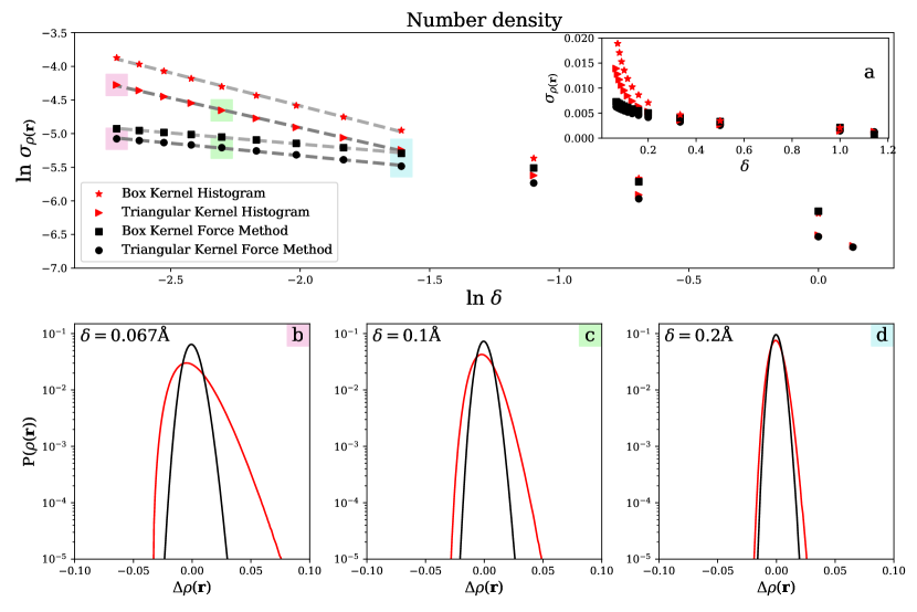
Figure 1: Panel a shows effect of changing $\delta$ on the standard deviation of the number densities for the histogram method (red stars for box kernel grids; red triangles for triangular kernel grids), and the force method (black squares for box kernel grids; black circles for triangular kernel grids), shown on a log-log scale in the main figure and on a linear scale in the inset. Panels b through d show the distributions of densities obtained for three delta values $\delta=$ 0.067Å, 0.1Å, and 0.2Å. The resulting distributions of $\Delta\rho({\bf r})$ for the histogram method (red) and the force method (black). The data points on panel a which correspond to the data in panels b through d are shown by colored squares. Dashed lines are linear fits to the data in the region from $\delta=0.2$ to $\delta=0.067$, with the slopes of these lines reported in Table 1.

Looking first to the general trend in standard deviations in Fig. 1a we observe, as one would expect, that the standard deviation in number density increases with decreasing $\delta$ for all four routes. This increase can be effectively approximated by a power law in all four cases and is thus linear on the log scale. However, for small voxels the rate of the increase in variance is diminished for the force method relative to the conventional histogram method, as anticipated from Borgis et al. Borgis et al. (2013). This is demonstrated by the much lower slope for the linear fits in Fig. 1 which are reported in Table 1.

The probability distributions of number densities in Fig. 1b through Fig. 1d (obtained using the triangular kernel) are narrower using the force method when contrasted to the histogram method for all values of $\delta$ (even though they converge for large voxels as shown in panel a). There is also a large difference in the forms of the distributions produced by the two methods, and how they change with decreasing $\delta$. For $\delta=0.2$ Å the form of both distributions is largely Gaussian. For the force method, this remains the same as $\delta$ decreases with a simple increase in width. In contrast, for the histogram method, the shape of the distributions changes with decreasing $\delta$. The peak of the distribution becomes shifted to values of $\Delta\rho(\mathbf{r})$ below 0, with a fat tail emerging at positive values, and the distribution becomes increasingly skewed. The asymmetry is due to the fact that in any one frame only 0.001%-0.02% of voxels are occupied, and as a voxel cannot be sampled fewer than zero times this leads to a warped distribution of density across the 3D grid. This shows a clear advantage for the use of the force method when extracting number densities.

We now turn to the distribution of the polarization density, illustrated in Fig. 2. As for number density, the standard deviation of polarization density is found to be similar for the two methods at larger values of $\delta$ but is shown to diverge with decreasing grid spacing. In panels b to d, we see again an increasing width of distributions with decreasing $\delta$, and that the distributions for the force-based method remain largely Gaussian. For the histogram-based method, however, the form of the distribution becomes increasingly less Gaussian with increasing $\delta$.

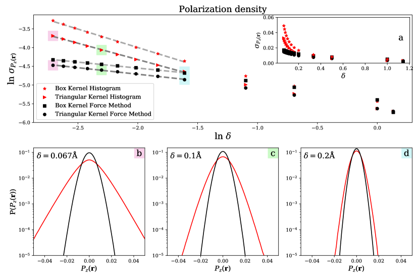
Figure 2: Panel a shows the effect of changing $\delta$ on the standard deviation of the polarization densities for the histogram method(red stars for box kernel grids; red triangles for triangular kernel grids), and the force method(black squares for box kernel grids; black circles for triangular kernel grids), shown on a log-log scale in the main figure and on a linear scale in the inset. Panels b through d show the distributions of densities obtained for three delta values $\delta=$ 0.067Å, 0.1Å, and 0.2Å. The resulting distributions of $P_{z}({\bf r})$ for the histogram method (red) and the force method (black). The data points on panel a which correspond to the data in panels b through d are shown by colored squares. Dashed lines are linear fit to the data in the region from $\delta=0.2$ to $\delta=0.067$, with the slopes of these lines reported in Table 1.

Table 1: The calculated slopes for the log-log plots of the standard deviation of densities against $\delta$ in Figs. 1 and 2.

Method	$\rho({\bf r})$	$P_{z}({\bf r})$
Box Kernel Histogram	-0.88	-0.87
Triangular Kernel Histogram	-0.98	-0.98
Box Kernel Force Method	-0.33	-0.32
Triangular Kernel Force Method	-0.37	-0.35

Figures 1 and 2 further demonstrate that for both densities, using the triangular kernel to compute the force or number density on the grid is superior to the box kernel (or conventional histogram), owing to the lower overall standard deviation for all values of $\delta$. Furthermore, the improvement gained by changing to a triangular kernel is greater for the histogram method than for the force method. However, it should be noted, as can be seen from Table 1 , that the standard deviation increases less with decreasing $\delta$ for the box kernel than for the triangular kernel for each method and density. From this point on, the more effective triangular kernel will be used, however it must be noted that this kernel decreases the improvement resulting from the new force method relative to the box kernel. Detailed results for the box kernel for the solvated water system are provided in the supplementary information.

Solvation: water around water

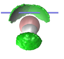
Figure 3: A rendered image showing the location of the characterization trace used for the 1D-analysis of number and polarization densities. In the case of polarization the $z$ axis is taken to run from the left to the right of this image. The isosurface corresponds to a number density $\rho({\bf r})=0.07$Å^-3 and illustrates the position of water molecules in the first solvation shell.

As previously mentioned, in order to explore the efficacy of the methodology for the extraction of 3D densities we consider first a simple model system consisting of a frozen water molecule in bulk water. In the following we analyze the 3D density along a single line of voxels in the direction ($z$) perpendicular to the molecular plane cutting the latter along the dipolar axis ($y$) at a position 0.6 Å away from the oxygen atom as shown in Fig. 3. The green isosurface defines the water molecules solvation shell. The traces that are taken along this line of voxels thus contain two peaks, and a void between them. When considering this plot from a more chemical perspective, we notice that the isosurface plot highlights three main regions of high density. The first region sits above the oxygen atom and consists of two lobes, corresponding to molecules donating a hydrogen bond to the constrained water molecule’s oxygen atom. The other two regions of high density correspond to hydrogen molecules receiving a hydrogen bond from the central molecule.

In the following, we analyze qualitatively the effect of grid spacing and trajectory length on the accuracy of the histogram and force methods, for the number density. We then proceed with polarization density before qualitatively examining the benefits of the force method for 3D representations of both types of density.

IV.0.1 Number density: effect of grid spacing

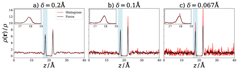
Figure 4: Number density extracted by means of the traditional histogram method (red) and the force method (black), for a single line of voxels as shown in Fig. 3. The data was extracted over the course of 4 ns with snapshots taken every 50 fs. This figure specifically explores the effect of varying grid spacing, $\delta=0.2,0.1$ and $0.067$Å for panels a to c, respectively. The insets with each figure are close-ups of the rising edge highlighted in blue in the main figure.

Fig. 4 shows the 3D number density along the trace illustrated in Fig. 3 for the histogram and force methods using grids with cubic voxels with edge length $\delta=$ 0.067 Å , 0.1 Å , and 0.2 Å. The latter is typical of the precision used in classical density functional theory studies of aqueous systems Ding et al. (2017); Zhao et al. (2011); Jeanmairet et al. (2013). In all cases, the density is reconstructed from the same configurations sampled every 50 fs from the 4 ns trajectory. The inset in each panel shows the form of the rising edge highlighted in blue in the main part of the panel. We first note that the basic form of each trace is identical regardless of the method and of the grid size. We observe the two main features in the form of the traces with a void centered on $z\,=$ 20 Å and two peaks present at 17.8Å and 22.2 Å. While for the considered number of configurations the two methods provide comparable results for the large voxels ($\delta$=0.2 Å), the noise increases much more dramatically with decreasing $\delta$ in the case of the histogram method. Importantly, while the results of the force method are qualitatively unchanged when decreasing $\delta$, those of the histogram method develop undesirable features such as a growing asymmetry between the two peaks, both of which are increasingly poorly described.

IV.0.2 Number density: effect of trajectory length

The previous analysis of grid spacings demonstrates the benefit of using the force method (compared to the histogram method) as the amount of data per voxel decreases. In practice, one is often interested in sampling the density for a fixed grid and the question to address is: how much data do we need to reach a given accuracy? We therefore examine, for a fixed grid size $\delta=0.1$ Å, the effect of the quality of the available data by considering several trajectory lengths (and sampling rates): an extremely long simulation and one each with lengths representative of typical classical and ab initio MD simulations.

As a reference, we report in Fig. 5a the results for a set of $3\text{\times}{10}^{6}$ configurations (from a 300 ns trajectory with samples every 100 fs). Even in that extreme case where data is not scarce, the benefit of the force method remains obvious. Decreasing the number of frames to $4\text{\times}{10}^{5}$ and increasing the correlations between frames (4 ns sampled every 10 fs), and even $5\text{\times}{10}^{4}$ (500 ps sampled every 10 fs) only makes this improvement more obvious.

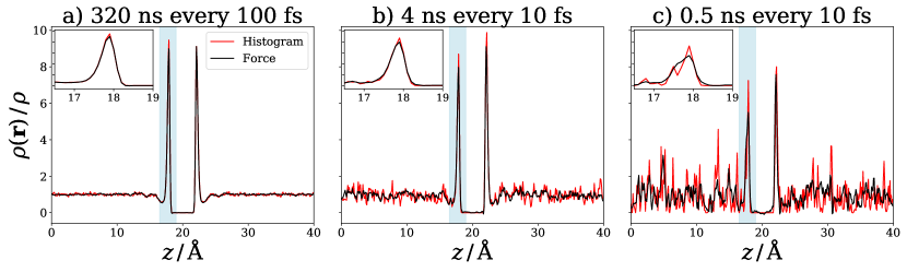
Figure 5: Number density extracted by means of the traditional histogram method (red) and the force method (black), for the single line of voxels shown in Fig. 3. The data was extracted on a grid with a spacing of 0.1Å with snapshots taken every 10 fs for the two shorter trajectories, and every 100 fs for the longer trajectory. This figure specifically explores the effect of varying trajectory length: 320, 4 and 0.5 ns for panels a, b and c, respectively. The insets are close-ups of the rising edges highlighted in blue in the main figures.

IV.0.3 Polarization density: effect of grid spacing

Thus far we have discussed only 3D number density (corresponding to $a_{i}=1$ in Eq. 19, and 21) that we extracted from the force density as in Borgiset al. Borgis et al. (2013). This is in itself novel as the methodology has not previously been applied to constrained molecules. We now turn to the other novel realization of this work, by considering a case $a_{i}\neq 1$, namely polarization ($a_{i}=\mathrm{p}_{z}$), i.e. the projection along the axis corresponding to the trace in Fig. 3.

Fig. 6 shows traces for the polarization density taken along the path shown in Fig 3, with the axis running from left to right. The figure has an identical layout to the previous cases with panels showing decreasing $\delta$ running from panel a to c. In all cases, we see positive polarization on approaching the constrained water molecule and negative polarization as we move away from that central water molecule. The plots should feature a center of inversion at point (20,0) due to the orthogonal relationship between the constrained water molecule’s $\sigma_{v}$ plane of symmetry and the traces that are plotted. The maintenance of this inversion symmetry will be a critical factor in accessing the accuracy of the results of both methods.

As was the case for the number density, the two methods produce near-identical results for the largest grid spacing ($\delta=$0.2 Å). We further note that at this grid spacing both peaks are roughly symmetric with respect to the expected center of inversion. However, as before, as we decrease the grid spacing (and thus the amount of data present per voxel) the force method is increasingly superior in extracting the polarization density. This is evidenced by the larger increase in the noise level with decreasing $\delta$ for the histogram method, as well as the poorer maintenance of the inversion symmetry in that case.

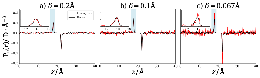
Figure 6: Polarization density extracted by means of the traditional histogram method (red) and the force method (black), for the single line of voxels as shown in Fig. 3. The data was extracted over the course of 4 ns with snapshots taken every 50 fs. This figure specifically explores the effect of varying grid spacing, $\delta=0.2,0.1$ and $0.067$Å for panels a to c, respectively. The insets are close-ups of the rising edge highlighted in blue on the main figures.

IV.0.4 Resolution of the 3D structure

Fig. 7 brings the implications of the previously observed trends into sharp relief. The isosurfaces are plotted for 3D densities for a grid size $\delta=$ 0.1 Å. The top and bottom two panels in the figure illustrate the 3D number and polarization density respectively extracted using both methods. The force method provides a large improvement on the histogram method in a number of key ways. As previously noted when looking at single traces and the density distributions without a constrained molecule, the noise away from the solvation shell is largely reduced with the new method, both for number and polarization densities. Likewise, we see a massive improvement in the resolution of the isosurfaces. This has large advantages for the further study and analysis of the 3D structure of the system, e.g. to identify basins of high density, a process that will become increasingly difficult with increasing roughness.

Fig. 7 additionally illustrates a feature specific to the polarization, namely a transition from positive polarization density to negative polarization density when passing through the molecular plane. For the force method, this transition is abrupt and occurs clearly at the location of the $\sigma_{v}$ molecular plane. This is a clear improvement on the histogram method where this boundary is poorly defined.

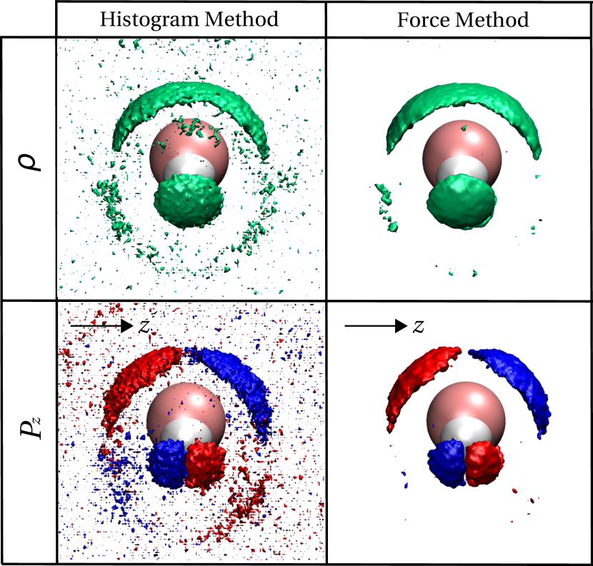
Figure 7: Isosurface plots for number density and polarization density for the two different methods of extraction of 3D densities. The green isosurface bounds the region where the number density is greater than 0.07 Å^-3 . For areas of polarization density blue (negative) and red (positive) bound less than -0.035 D$\cdot$Å^-3 and greater than +0.035 D$\cdot$Å^-3 respectively.

IV.1 Lysozyme Solvation 4 ns

After the demonstration of the success of the force method on a somewhat academic first case, we finally illustrate its relevance on a physically more appealing example, namely the lysozyme protein. In contrast with the more symmetric constrained water system, the globular protein studied here cannot be well understood by studying the polarization density. Instead, we study here the 3D charge density, where the value of $a_{i}$ in Eq. (19) is taken to be $q_{i}$. In line with the previously described equations for rigid molecules, the position and charge of each atom is considered when calculating the charge density, but the relevant force is the total force acting on the rigid molecule (see Eqs. 21 and 16).

The isosurfaces plots in Fig. 8 show the potential of the new method in the understanding of solvation. Firstly, in both cases, number and charge density, the histogram method leads to a large amount of noise away from the protein molecules surface. Beyond making the image less aesthetically pleasing this leads to two further problems in the density extracted by the histogram method relative to the force method. This noise is symptomatic of a poor baseline that will cause difficulties for any subsequent analyses that need to be performed. Further to this, it causes a large difficulty in resolving the shape of the solvation shell at its outer boundary. In the case of the charge density, we see even better the improvements obtained thanks to the new method. These lobes of positive and negative charge density allow one to identify the directionality of the coordination by water molecules at each site on the protein. Overall these results show a massive improvement in the resolution of the isosurfaces and show the clear applicability of this methodology to real systems beyond the model systems intensively studied in the previous sections.

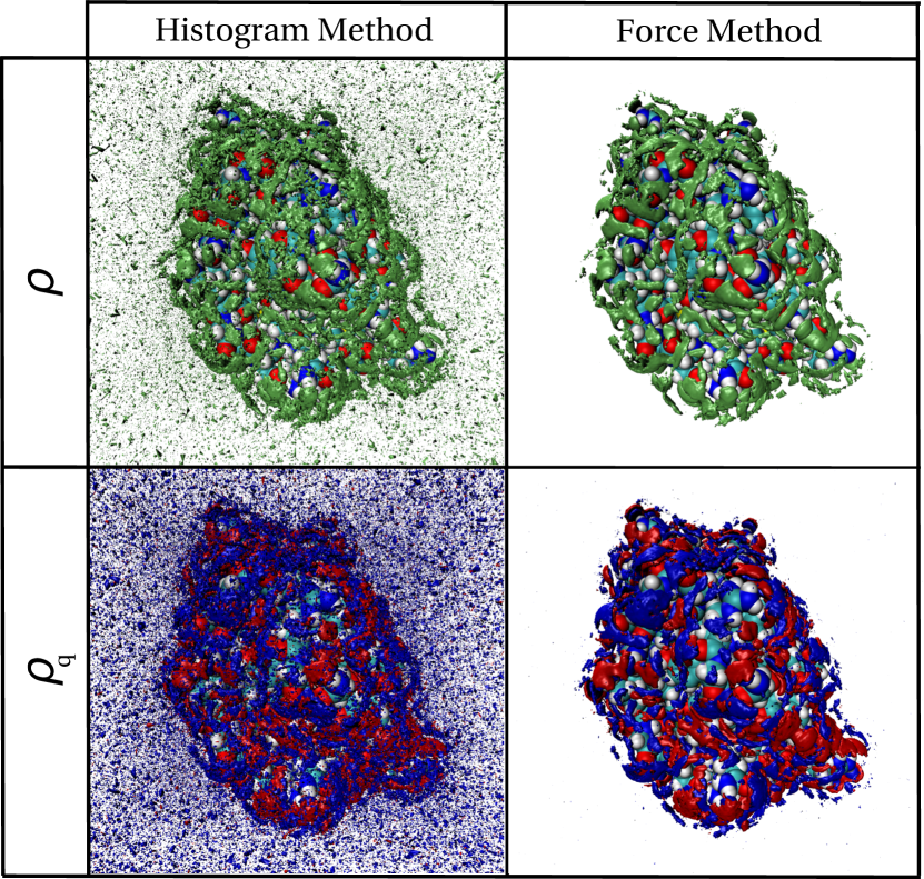
Figure 8: Isosurface plots for number density, $\rho$, and charge density, $\rho_{q}$, for the two methods of extraction of 3D densities. The green isosurfaces bound the regions where the number density greater than 0.1 Å^-3. The red (positive) and blue (negative) surfaces bound areas where the magnitude of the charge density exceeds $\pm$0.1 $e\cdot$Å^-3.

V Conclusion

We have presented a reduced variance method for the calculation of not only 3D number densities but also other generic 3D densities by molecular simulations. The data collection of the local force densities instead of the number densities and their post-processing is as easy and inexpensive as in the conventional density histograms collection, requiring only an extra 3D-FFT at the end to transform from force densities to number densities. We have further extended this method to the common case of rigid molecules described by distance constraints, such as the popular SPC/E or TIPnP water models. This new force density method appears more or less statistically equivalent to the conventional method for voxel sizes above $\delta=0.2$ Å, but is much more efficient below that size. Furthermore, the variance of the results depends only slightly on $\delta$. This improved statistical efficiency makes it possible to reach a given prescribed variance of the computed densities with shorter trajectories, thus at a reduced simulation cost. We clearly illustrated for the water structure around a small molecular solute (specifically water in water) as well as for a complex molecular object (lysozyme protein), that for a given simulation time the force method enables better resolution of the 3D structure, including individualization of the density peaks and equalization of the background and that it leads to a much clearer visualization (figures 7 and 8). We thus believe that the method has already a wide range of useful applications in many fields when it comes to characterizing by simulation the molecular solvation structure of complex biomolecular or solid-liquid interfaces. Several theoretical/technical challenges remain, such as a possible optimal mixing between density histograms and force histograms, or the expansion from force densities to force divergence densities evoked in Ref. 24. Further work along these lines is underway.

Supplementary Material

Versions of graphs contained within the water molecule solvation section are presented for the box kernel in the supplementary information.

Supporting information: Computing three-dimensional densities from force densities improves statistical efficiency

Water number density around water: results using a box kernel

In the main paper a triangular kernel was used to obtain the grids of number density, polarization density, force density, and the polarization density equivalent of the force density. The triangular kernel was employed in order to give the histogram method the best possible chance against the force method, as it significantly minimizes the effects of digitization on the resulting histogram. However when trying to obtain a 3 dimensional density one might naively prefer to use a box kernel, which is the conventional way of taking 3D histograms. In Fig. S1 we present the results obtained for the number density around a solvated water molecule obtain using a box kernel (this figure is identical to Fig. 4 of the main paper but for the change of kernel). The new force method provides the ability for reduced variance extraction of number densities particularly at lower values of $\delta$. One additional effect of the application of the force method to box kernel grids is that it removes the digitization of the data which is observed for the direct binning of positions. This is in accord with the analysis of density fluctuations in three dimensional space, which showed decreased standard deviation with the triangular kernel for exactly this reason.

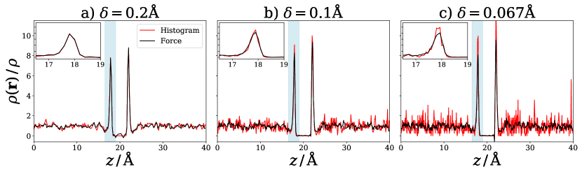
Figure S1: Number density extracted by means of the traditional histogram method (red) and the force method (black), for a single line of pixels as shown in Fig. 3 of the main paper. The data was extracted over the course of 4 ns with snapshots taken every 50 fs. This figure specifically explores the effect of varying grid spacing, $\delta=0.2,0.1$ and $0.067$Å for panels a to c, respectively. The insets within each figure are close ups of the rising edge highlighted in blue in the main figure. In contrast with Fig. 4 in the main paper a box kernel was used to extract the grid in this example.

We now move on to compare the results of the force method using both triangular and box kernels displayed in Fig. S2. In the main paper the analysis of the density fluctuation showed a slightly smaller noise level for the triangular kernel. The difference in noise across all values of $\delta$ for the two methods is however not the most obvious difference, it is more apparent that the grids formed using a triangular kernel provide better resolution of the edge of the void.

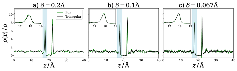
Figure S2: Number density extracted by means of the force method for grids created using triangular (black), and box (green) kernels for a single line of pixels as shown in Fig. 3 of the main paper. The data was extracted over the course of 4 ns with snapshots taken every 50 fs. This figure specifically explores the effect of varying grid spacing, $\delta=0.2,0.1$ and $0.067$Å for panels a to c, respectively. The insets within each figure are close ups of the rising edge highlighted in blue in the main figure.

Water polarization density around water: results using a box kernel

Fig. S3 shows the traces for the polarization density, using both the histogram and force methods, using grids obtained with the box kernel. In this example we see, as in the main paper and the number density, that the form of the traces is roughly the same for the two methods. The amount of noise is greater for the traditional method than for the force method for the two finer grids, but, as before, is similar for $\delta=0.2$ Å. As in the case of number density, the difference in the ability to resolve the void becomes even more apparent on studying Fig. S4 which shows the results obtained with force method for the two kernels. A distinct fish hook feature is observed on the second rising edge for $\delta=$0.067 Å for the box kernel which isn’t present for the triangular kernel.

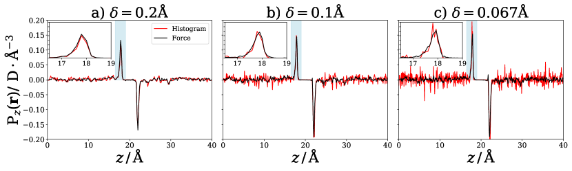
Figure S3: Polarization densities extracted by means of the traditional histogram method (red) and the force method (black). The polarization density is shown for a single line of pixels as shown in Fig. 3 of the main paper. The data was extracted over the course of 4 ns with snapshots taken every 50 fs. This figure specifically explores the effect of varying grid spacing, $\delta=0.2,0.1$ and $0.067$Å for panels a to c, respectively. The insets within each figure are close ups of the rising edge highlighted in blue in the main figure. In contrast with Fig. 6 in the main paper a box kernel was used to obtain the grid in this example.

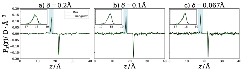
Figure S4: Polarization density extracted by means of the force method for grids created using triangular (black), and box (green) kernels for a single line of pixels as shown in Fig. 3 of the main paper. The data was extracted over the course of 4 ns with snapshots taken every 50 fs. This figure specifically explores the effect of varying grid spacing, $\delta=0.2,0.1$ and $0.067$Å for panels a to c, respectively. The insets within each figure are close ups of the rising edge highlighted in blue in the main figure.

References

- Abel et al. (2007) R. Abel, R. A. Friesner, T. Young, B. Kim, and B. J. Berne, “Motifs for molecular recognition exploiting hydrophobic enclosure in protein–ligand binding,” Proc. Natl. Acad. Sci. 104, 808–813 (2007).
- Abel et al. (2008) R. Abel, T. Young, R. Farid, B. J. Berne, and R. A. Friesner, “Role of the Active-Site Solvent in the Thermodynamics of Factor Xa Ligand Binding,” J. Am. Chem. Soc. , 2817–2831 (2008).
- Nguyen, Kurtzman Young, and Gilson (2012) C. N. Nguyen, T. Kurtzman Young, and M. K. Gilson, “Grid inhomogeneous solvation theory: Hydration structure and thermodynamics of the miniature receptor cucurbit[7]uril,” J. Chem. Phys. 137, 973–980 (2012).
- Nguyen et al. (2014) H. T. Nguyen, S. A. Pabit, S. P. Meisburger, L. Pollack, and D. A. Case, “Accurate small and wide angle x-ray scattering profiles from atomic models of proteins and nucleic acids,” J. Chem. Phys. 141 (2014).
- Marchi (2016) M. Marchi, “A first principle particle mesh method for solution SAXS of large bio-molecular systems,” J. Chem. Phys. 145 (2016).
- Altan et al. (2018) I. Altan, D. Fusco, P. V. Afonine, and P. Charbonneau, “Learning about Biomolecular Solvation from Water in Protein Crystals,” J. Phys. Chem. B 122, 2475–2486 (2018).
- Wall et al. (2019) M. E. Wall, G. Calabró, C. I. Bayly, D. L. Mobley, and G. L. Warren, “Biomolecular Solvation Structure Revealed by Molecular Dynamics Simulations,” J. Am. Chem. Soc. 141, 4711–4720 (2019).
- Klausen, Fuhs, and Dong (2016) L. H. Klausen, T. Fuhs, and M. Dong, “Mapping surface charge density of lipid bilayers by quantitative surface conductivity microscopy,” Nature Communications 7, 12447 (2016).
- José Segura et al. (2013) J. José Segura, A. Elbourne, E. J. Wanless, G. G. Warr, K. Voïtchovsky, and R. Atkin, “Adsorbed and near surface structure of ionic liquids at a solid interface,” Physical Chemistry Chemical Physics 15, 3320–3328 (2013).
- Elbourne et al. (2015) A. Elbourne, S. McDonald, K. Voïchovsky, F. Endres, G. G. Warr, and R. Atkin, “Nanostructure of the Ionic Liquid–Graphite Stern Layer,” ACS Nano 9, 7608–7620 (2015).
- Docampo-Álvarez et al. (2016) B. Docampo-Álvarez, V. Gómez-González, H. Montes-Campos, J. M. Otero-Mato, T. Méndez-Morales, O. Cabeza, L. J. Gallego, R. M. Lynden-Bell, V. B. Ivaništšev, M. V. Fedorov, and L. M. Varela, “Molecular dynamics simulation of the behaviour of water in nano-confined ionic liquid–water mixtures,” J. Phys.: Condens. Matter 28, 464001 (2016).
- Kornyshev and Qiao (2014) A. A. Kornyshev and R. Qiao, “Three-Dimensional Double Layers,” J. Phys. Chem. C 118, 18285–18290 (2014).
- Merlet et al. (2014) C. Merlet, D. T. Limmer, M. Salanne, R. van Roij, P. A. Madden, D. Chandler, and B. Rotenberg, “The Electric Double Layer Has a Life of Its Own,” J. Phys. Chem. C 118, 18291–18298 (2014).
- Jeanmairet et al. (2019) G. Jeanmairet, B. Rotenberg, M. Levesque, D. Borgis, and M. Salanne, “A molecular density functional theory approach to electron transfer reactions,” Chemical Science 10, 2130–2143 (2019).
- Merlet et al. (2012) C. Merlet, B. Rotenberg, P. A. Madden, P.-L. Taberna, P. Simon, Y. Gogotsi, and M. Salanne, “On the molecular origin of supercapacitance in nanoporous carbon electrodes,” Nature Materials 11, 306–310 (2012).
- Merlet et al. (2013) C. Merlet, C. Péan, B. Rotenberg, P. A. Madden, B. Daffos, P.-L. Taberna, P. Simon, and M. Salanne, “Highly confined ions store charge more efficiently in supercapacitors,” Nature Communications 4, 2701 (2013).
- Kondrat et al. (2012) S. Kondrat, C. R. Pérez, V. Presser, Y. Gogotsi, and A. A. Kornyshev, “Effect of pore size and its dispersity on the energy storage in nanoporous supercapacitors,” Energy & Environmental Science 5, 6474–6479 (2012).
- Simoncelli et al. (2018) M. Simoncelli, N. Ganfoud, A. Sene, M. Haefele, B. Daffos, P.-L. Taberna, M. Salanne, P. Simon, and B. Rotenberg, “Blue Energy and Desalination with Nanoporous Carbon Electrodes: Capacitance from Molecular Simulations to Continuous Models,” Phys. Rev. X 8, 021024 (2018).
- Yoshida et al. (2009) N. Yoshida, T. Imai, S. Phongphanphanee, A. Kovalenko, and F. Hirata, “Molecular recognition in biomolecules studied by statistical-mechanical integral-equation theory of liquids,” J. Phys. Chem. B 113, 873–886 (2009).
- Stumpe et al. (2011) M. C. Stumpe, N. Blinov, D. Wishart, A. Kovalenko, and V. S. Pande, “Calculation of local water densities in biological systems: A comparison of molecular dynamics simulations and the 3D-RISM-KH molecular theory of solvation,” J. Phys. Chem. B 115, 319–328 (2011).
- Ding et al. (2017) L. Ding, M. Levesque, D. Borgis, and L. Belloni, “Efficient molecular density functional theory using generalized spherical harmonics expansions,” J. Chem. Phys. 147 (2017).
- Zhao et al. (2011) S. Zhao, R. Ramirez, R. Vuilleumier, and D. Borgis, “Molecular density functional theory of solvation: From polar solvents to water,” J. Chem. Phys. 134 (2011).
- Jeanmairet et al. (2013) G. Jeanmairet, M. Levesque, R. Vuilleumier, and D. Borgis, “Molecular density functional theory of water,” J. Phys. Chem. Lett. 4, 619–624 (2013).
- Borgis et al. (2013) D. Borgis, R. Assaraf, B. Rotenberg, and R. Vuilleumier, “Computation of pair distribution functions and three-dimensional densities with a reduced variance principle,” Molecular Physics 111, 3486–3492 (2013).
- de las Heras and Schmidt (2018) D. de las Heras and M. Schmidt, “Better Than Counting: Density Profiles from Force Sampling,” Phys. Rev. Lett. 120, 218001 (2018).
- Purohit, Schultz, and Kofke (2019) A. Purohit, A. J. Schultz, and D. A. Kofke, “Force-sampling methods for density distributions as instances of mapped averaging,” Molecular Physics 0, 1–8 (2019).
- Schultz and Kofke (2019) A. J. Schultz and D. A. Kofke, “Alternatives to conventional ensemble averages for thermodynamic properties,” Current Opinion in Chemical Engineering Frontiers of Chemical Engineering: Molecular Modeling, 23, 70–76 (2019).
- Ciccotti, Kapral, and Vanden-Eijnden (2005) G. Ciccotti, R. Kapral, and E. Vanden-Eijnden, “Blue Moon Sampling, Vectorial Reaction Coordinates, and Unbiased Constrained Dynamics,” ChemPhysChem 6, 1809–1814 (2005).
- Berendsen, Grigera, and Straatsma (1987) H. J. C. Berendsen, J. R. Grigera, and T. P. Straatsma, “The missing term in effective pair potentials,” The Journal of Physical Chemistry 91, 6269–6271 (1987).
- Abraham et al. (2015) M. J. Abraham, T. Murtola, R. Schulz, S. Páll, J. C. Smith, B. Hess, and E. Lindahl, “GROMACS: High performance molecular simulations through multi-level parallelism from laptops to supercomputers,” SoftwareX 1-2, 19–25 (2015).
- Martìnez et al. (2009) L. Martìnez, R. Andrade, E. G. Birgin, and J. M. Martínez, “PACKMOL: A Package for Building Initial Configurations for Molecular Dynamics Simulations,” Journal of Computational Chemistry 30, 2157–2164 (2009).
- Darden, York, and Pedersen (1993) T. Darden, D. York, and L. Pedersen, “Particle mesh Ewald: An Nlog(N) method for Ewald sums in large systems,” J. Chem. Phys. 98, 10089–10092 (1993).
- Posch, Hoover, and Vesely (1986) H. A. Posch, W. G. Hoover, and F. J. Vesely, “Canonical dynamics of the Nos\’e oscillator: Stability, order, and chaos,” Phys. Rev. A 33, 4253–4265 (1986).
- Lemkul (2018) J. Lemkul, “From Proteins to Perturbed Hamiltonians: A Suite of Tutorials for the GROMACS-2018 Molecular Simulation Package [Article v1.0],” Living Journal of Computational Molecular Science 1, 5068 (2018).
- Jorgensen, Maxwell, and Tirado-Rives (1996) W. L. Jorgensen, D. S. Maxwell, and J. Tirado-Rives, “Development and Testing of the OPLS All-Atom Force Field on Conformational Energetics and Properties of Organic Liquids,” J. Am. Chem. Soc. 118, 11225–11236 (1996).
- Bussi, Donadio, and Parrinello (2007) G. Bussi, D. Donadio, and M. Parrinello, “Canonical sampling through velocity rescaling,” J. Chem. Phys. 126, 014101 (2007).
- Berendsen et al. (1984) H. J. C. Berendsen, J. P. M. Postma, W. F. van Gunsteren, A. DiNola, and J. R. Haak, “Molecular dynamics with coupling to an external bath,” J. Chem. Phys. 81, 3684–3690 (1984).
- Richard J. Gowers et al. (2016) Richard J. Gowers, Max Linke, Jonathan Barnoud, Tyler J. E. Reddy, Manuel N. Melo, Sean L. Seyler, Jan Domański, David L. Dotson, Sébastien Buchoux, Ian M. Kenney, and Oliver Beckstein, “MDAnalysis: A Python Package for the Rapid Analysis of Molecular Dynamics Simulations,” in Proceedings of the 15th Python in Science Conference, edited by Sebastian Benthall and Scott Rostrup (2016) pp. 98 – 105.
- Michaud-Agrawal et al. (2011) N. Michaud-Agrawal, E. J. Denning, T. B. Woolf, and O. Beckstein, “MDAnalysis: A toolkit for the analysis of molecular dynamics simulations,” Journal of Computational Chemistry 32, 2319–2327 (2011).