Reconstructing $f(T)$ modified gravity from ECHDE and ECNADE models

Abstract

We investigate alternative candidates to dark energy that can explain the current state of the universe in the framework of the generalized teleparallel theory of gravity $f(T)$ where $T$ denotes the torsion scalar. To achieve this, we carried out a series of reconstruction taking into account to the ordinary and entropy-corrected versions of the holographic and new agegraphic dark energy models. These models used as alternative to dark energy in the literature in order describe the current state of our universe. It is remarked that the models reconstructed indicates behaviors like phantom or quintessence models. Furthermore, we also generated the EoS parameters associated to entropy-corrected models and we observed a transition phase between quintessence state and phantom state as showed by recent observational data. We also investigated on the stability theses models and we created the $\{r-s\}$. The behavior of certains physical parameters as speed of sound and the Statefinder parameters are compatible with current observational data.

Keywords: teleparallel gravity, ECHDE, ECNADE

I Introduction

Some irrefutable evidence such as debamba1 ; debamba2 ; debamba3 ; debamba4 ; debamba5 ; debamba6 indicate that the universe our universe is experiencing an accelerated expansion. A possible candidate responsible for this current behavior of the universe is a mysterious energy with negative pressure which the origin and nature always stay unelucidated. For reasons of incompatibility with the experimental data, several DE models proposed for this purpose have proved unsuccessfulPadmanabhan ; Copeland ). Based on the holographic principle, Horava ; Hooft ; Fischler , a promising DE candidate so-called holographic DE (HDE) was proposed. For a good review see about HDE, see cohen ; Li . Interesting results have been obtained in the literature Enqvist ; Elizalde2 ; Guberina1 ; Guberina2 ; Karami1 .

It is no longer necessary to demonstrate the importance of the black hole entropy $S_{\rm BH}$ in the derivation of holographic dark energy. Followingmodak , this entropy-area relation $S_{\rm BH}=A/(4G)$, where $A\sim L^{2}$ is the area of horizon of black hole may undergo change as

$$S_{\rm BH}=\frac{A}{4G}+\tilde{\alpha}\ln{\frac{A}{4G}}+\tilde{\beta},$$ (1)

which the parameters $\tilde{\alpha}$ and $\tilde{\beta}$ are dimensionless constants of order unity. These modifications have been subject of a large study in the framework loop quantum gravity (LQG) HW . In this renewed attention that wei proposed the energy density of the entropy-corrected dark energy (ECHDE) modelHW . Besides the holographic dark energy, CaiCai suggested a new idea so-called agegraphic dark energy in order to to describe current behavior of the universe. This model has been subject of several discussions in literatureKar1 ; Maz . It should be noted that this model can not describe the matter-dominated epoch. In order to correct the insufficiency, the new agegraphic dark energy (NADE) model was proposed by Wei $\&$ Cai Wei1 and interesting results can be found in Wei2 ; Kim ; Kim11 ; Sheykhi . Thereafter, Using a similar method of modification of ECHDE model, wey suggested a version corrected so-called entropy-corrected NADE (ECNADE) HW which has been investigated by Karami2 .

Another approach to better understand this mysterious energy is to modify standard theories of gravity such as the General Relativity or the equivalent theory so-called Teleparallel Theory. Some gravity theories proposed as ma1 ; ma2 ; mj1 ; mj5 . Among these proposed gravity theories, one caught our attention. This is $f(T)$ gravity as the modified version of the Teleparallel Theory. Interesting results have been found there st1 - st2 .

In view of $f(T)$ gravity as an alternative theory of mystery candidate, it is necessary to investigate how this theory can describe the Entropy-Corrected holographic Dark Energy (ECHDE) and the Entropy-Corrected New Agegraphic Dark Energy (ECNADE) models. The paper is organized as follows. In sectionII, we present the generality on $f(T)$ gravity. In sections III to VI we present a series of reconstruction taking into account to the ordinary and entropy-corrected versions of the holographic and new agegraphic dark energy models. stability analysis, Statefinder parameters and the reconstruction in de Sitter space will be presented through the sections VII, VIII, LABEL:sec9 and the conclusion is presented in section IX.

II Generality on $f(T)$ gravity

Unlike General Relativity and its modified versions where the gravitational interaction is described by making use the Levi-Civita’s connection, the teleparallel theory and its modified versions describe the gravitational interaction via the curvatureless Weizenbock’s connection, whose non-null torsion defined by

$$\Gamma^{\lambda}_{\mu\nu}=e^{\;\;\lambda}_{i}\partial_{\mu}e^{i}_{\;\;\nu}=-e^{i}_{\;\;\mu}\partial_{\nu}e_{i}^{\;\;\lambda}.$$ (2)

Thus, we can define respectively torsion and the contorsion, the torsion scalar as

$$T^{\lambda}_{\;\;\;\mu\nu}=\Gamma^{\lambda}_{\mu\nu}-\Gamma^{\lambda}_{\nu\mu},$$ (3)

$$K^{\mu\nu}_{\;\;\;\;\lambda}=-\frac{1}{2}\left(T^{\mu\nu}_{\;\;\;\lambda}-T^{\nu\mu}_{\;\;\;\;\lambda}+T^{\;\;\;\nu\mu}_{\lambda}\right)\,\,,$$ (4)

$$T=T^{\lambda}_{\;\;\;\mu\nu}S^{\;\;\;\mu\nu}_{\lambda}\,.$$ (5)

Now, we define the action of the modified version of TG whose Lagrangian is an algebraic function depending of the torsion.

$$S=\int e\left[\frac{f(T)}{2\kappa^{2}}+\mathcal{L}_{m}\right]d^{4}x\,,$$ (6)

where $\kappa^{2}=8\pi G$ is the usual gravitational coupling constant. The following equations of motion are obtained by varying the the action (6) via the tetrads

$$S^{\;\;\;\nu\rho}_{\mu}\partial_{\rho}Tf_{TT}+[e^{-1}e^{i}_{\;\;\mu}\partial_{\rho}(ee^{\;\;\mu}_{i}S^{\;\;\;\nu\lambda}_{\alpha})+T^{\alpha}_{\;\;\;\lambda\mu}S^{\;\;\;\nu\lambda}_{\alpha}]f_{T}+\frac{1}{4}\delta^{\nu}_{\mu}f=\frac{\kappa^{2}}{2}\mathcal{T}^{\nu}_{\mu}\,,$$ (7)

where $\mathcal{T}^{\nu}_{\mu}$ is the energy momentum tensor, $f_{T}=df(T)/dT$ and $f_{TT}=d^{2}f(T)/dT^{2}$ the first and second derivative of $f(T)$ with respect to $T$. Considering a flat $FLRW$ cosmologies, the torsion scalar yields to

$$T=-6H^{2},$$ (8)

where $H=\dot{a}/a$ denotes the Hubble parameter. Thus, the usual Friedmann equations become

$$H^{2} = \frac{8\pi G}{3}(\rho+\rho_{T}),$$ (9)

$$2\dot{H}+3H^{2} = -\frac{8\pi G}{3}(p+p_{T}),$$ (10)

where

$$\rho_{T} = \frac{1}{16\pi G}[2Tf_{T}-f-T],$$ (11)

$$p_{T} = \frac{1}{16\pi G}[2\dot{H}(4Tf_{TT}+2f_{T}-1)]-\rho_{T}.$$ (12)

This above quantities define respectively the torsion contributions to the energy density and pressure who checks the following continuity equation.

$$\dot{\rho}_{T}+3H(\rho_{T}+p_{T}) = 0.$$ (13)

We can notice for the null torsion contribution, the general relativity (Teleparallel Gravity) recoved. In order to preserve the modified nature of the gravity and by make using Eqs. (11) and (12), we can write the effective torsion equation of state as Nozari

$$\omega_{T}\equiv\frac{p_{T}}{\rho_{T}}=-1-\frac{4\dot{H}\Big{(}2Tf^{\prime\prime}(T)+f^{\prime}(T)-1\Big{)}}{T-2Tf^{\prime}(T)+f(T)}.$$ (14)

Considering a universe for a slow contribution of the matter, we can note that the Eq. (9) yields

$$\frac{3}{k^{2}}H^{2}=\rho_{T}.$$ (15)

Thus, the EoS parameter can be obtained in the same conditions as previously by making use (14) and (13)

$$\omega_{T}=-1-\frac{2\dot{H}}{3H^{2}}.$$ (16)

We can remark that the first derivative of the Hubble parameter is positive $\dot{H}>0$ for an accelerating expanded phantom-like universe ($\omega_{T}<-1$) and negative $\dot{H}<0$ for an accelerated expanded quintessence-like one $\omega_{T}>-1$. Based on the torsion contribution and any class of scale factor $a=a(t)$, one can perform a series of reconstruction taking according to the ordinary and entropy-corrected versions of the holographic and new agegraphic dark energy models. Among the existing series of classes of scale factors, we will focus on two classes habitually used in modified gravity to describe the process of the accelerating universe Nojiri .

The first category of scale factor is defined by Nojiri ; Sadjadi

$$a(t)=a_{0}\,(t_{s}-t)^{-h},\quad t\leq t_{s},\quad h>0.$$ (17)

By considering Eqs. (8) and (17), the Hubble parameter becomes

$$H=\frac{h}{t_{s}-t}=\left[\frac{-T}{6}\right]^{1/2},~{}~{}~{}\dot{H}=H^{2}/h,$$ (18)

which shows that

The model (17) the model responds perfectly to a model that describes an accelerating expanded phantom-like universe $\dot{H}=H^{2}/h>0$ and this is also the reason why the said model is habitually so-called the phantom-like scale factor.

On the other hand, we can define the second category of scale factor as Nojiri

$$a(t)=a_{0}t^{h},~{}~{}~{}h>0,$$ (19)

and yields to

$$H=\frac{h}{t}=\left[\frac{-T}{6}\right]^{1/2},~{}~{}~{}\dot{H}=-H^{2}/h,$$ (20)

which $\dot{H}<0$. We can remark that the model (19) indicate a accelerating expanded quintessence-like universe. In order to give a cosmological interpretation, we plotted versus redshift $z=\frac{a_{0}}{a}-1$. Thus, for the first category of scale factor (17) become

$$T=\frac{-6h^{2}}{(1+z)^{\frac{2}{h}}},$$ (21)

on the other hand the second category of scale factor (19) yields

$$T=-6h^{2}(1+z)^{\frac{2}{h}}.$$ (22)

In the following sections, we present a series of reconstruction taking into account to the ordinary and entropy-corrected versions of the holographic and new agegraphic dark energy models and by making use of of two categories of scale factors previously described.

III $f(T)$ reconstruction from HDE model

FollowingLi , the holographic dark energy model in a spatially flat universe is characterized by a density given by

$$\rho_{\Lambda}=\frac{3c^{2}}{k^{2}R_{h}^{2}},$$ (23)

where $c$ is a numerical constant introduced for convenience. The latest observational data for a flat universe show that this constant worth $c=0.818_{-0.097}^{+0.113}$ Li6 . We define radius of the event horizon $R_{h}$ as

$$R_{h}=a\int_{t}^{\infty}\frac{{\rm d}t}{a}=a\int_{a}^{\infty}\frac{{\rm d}a}{Ha^{2}}.$$ (24)

Thus, we can evaluate for first category of scale factor (17) the future event horizon $R_{h}$ by making use Eq. (18)

$$R_{h}=a\int_{t}^{t_{s}}\frac{{\rm d}t}{a}=\frac{t_{s}-t}{h+1}=\frac{h}{h+1}\sqrt{\frac{-6}{T}}.$$ (25)

Substituting Eq. (25) into (23) one can obtain

$$\rho_{\Lambda}=\frac{-3c^{2}(h+1)^{2}}{6k^{2}h^{2}}T.$$ (26)

Replacing Eq. (26) in the differential equation (11), i.e. $\rho_{T}=\rho_{\Lambda}$, yields the following solution

$$f(T)=\frac{\left(h^{2}-c^{2}(1+h)^{2}\right)T}{h^{2}}+\sqrt{T}C_{1},$$ (27)

where $C_{1}$ is integration constant. For more consistency, the constants have been to be determined and to to do so, we impose the initial conditions, assuming the assumption according to what, at present time, the holographic model must recover the usual $\Lambda$CDM one, that is

$$\left(f\right)_{t=t_{0}}=T_{0}-2\Lambda\;\;,\quad\quad\left(\frac{df}{dt}\right)_{t=t_{0}}=\left(\frac{dT}{dt}\right)_{t=t_{0}}\;,$$ (28)

where the subscript $t_{0}$ and $T_{0}$ denote the present time and the related value of the torsion scalar, respectively.

Making use of the initial conditions (28), one gets

$$C_{1}=\frac{-2h^{2}\Lambda+c^{2}(1+h)^{2}T_{0}}{h^{2}\sqrt{T_{0}}}$$ (29)

such that the algebraic holographic dark energy model reads

$$f(T)=\frac{\left(h^{2}-c^{2}(1+h)^{2}\right)T}{h^{2}}+\frac{\sqrt{T}\left(-2h^{2}\Lambda+c^{2}(1+h)^{2}T_{0}\right)}{h^{2}\sqrt{T_{0}}}\;.$$ (30)

We can obtain easily the EoS parameter for $f(T)$-gravity according to the HDE model by replacing Eq. (30) into (14) and making use (18),

$$\omega_{T}=-1-\frac{2}{3h},~{}~{}~{}h>0,$$ (31)

which data indicates to a accelerating expanded phantom-like universe, i.e. $\omega_{T}<-1$. We see also that the EoS parameter $\omega_{T}$ according to the observational data Copeland .

Considering the second class of scale factor (19) and (20), the future event horizon $R_{h}$ yields to

$$R_{h}=a\int_{t}^{\infty}\frac{{\rm d}t}{a}=\frac{t}{h-1}=\frac{h}{(h-1)}\sqrt{\frac{-6}{T}},~{}~{}~{}h>1.$$ (32)

Also, using the same procedure, we can determine

$$f(T)=\frac{\left(-c^{2}(-1+h)^{2}+h^{2}\right)T}{h^{2}}+\frac{\sqrt{T}\left(-2h^{2}\Lambda+c^{2}(-1+h)^{2}T_{0}\right)}{h^{2}\sqrt{T_{0}}},$$ (33)

and

$$\omega_{T}=-1+\frac{2}{3h},~{}~{}~{}h>1.$$ (34)

We can note that the EoS parameter satisfies $-1<\omega_{T}<-1/3$ which data indicates to a accelerating expanded quintessence-like universe.

IV $f(T)$ reconstruction from ECHDE model

In this section, we present the modified version of energy density suggested by Wei HW , so-called (ECHDE). This model is given by

$$\rho_{\Lambda}=\frac{3c^{2}}{k^{2}R_{h}^{2}}+\frac{\alpha}{R_{h}^{4}}\ln\left(\frac{R_{h}^{2}}{k^{2}}\right)+\frac{\beta}{R_{h}^{4}},$$ (35)

with two dimensionless constants $\alpha$ and $\beta$. unity. One note that the HDE model is recoved for $\alpha=\beta=0$. Thus, the last two terms in Eq. (35) constitute the corrections made to the HDE model. When the universe becomes large, ECHDE reduces to the ordinary HDE HW .

Considering the first category of scale factor (17) and making use the Eq.(25), (35), the density corresponding to entropy-corrected HDE becomes

$$\rho_{\Lambda}=\frac{(1+h)^{2}T\left((1+h)^{2}T\beta-\frac{18c^{2}h^{2}}{\kappa^{2}}+(1+h)^{2}T\alpha\text{Log}\left[-\frac{6h^{2}}{(1+h)^{2}T\kappa^{2}}\right]\right)}{36h^{4}}.$$ (36)

Thus, the algebraic function according to ECHDE model yields

$$f(T) = \sqrt{T}C_{1}+\frac{T\left(-162h^{2}(c+(-1+c)h)(c+h+ch)\right)}{162h^{4}}$$ (37)

$$+ \;\;\frac{T\left((1+h)^{4}T(2\alpha+3\beta)\kappa^{2}+3(1+h)^{4}T\alpha\kappa^{2}\text{Log}\left[-\frac{6h^{2}}{(1+h)^{2}T\kappa^{2}}\right]\right)}{162h^{4}},$$ (38)

where $C_{1}$ is constant. By making use the boundary conditions (28), we can determine $C_{1}$ as

$$C_{1}=-\frac{2\Lambda}{\sqrt{T_{0}}}+\frac{c^{2}(1+h)^{2}\sqrt{T_{0}}}{h^{2}}-\frac{(1+h)^{4}\kappa^{2}\left(2\alpha+3\beta+3\alpha\text{Log}\left[-\frac{6h^{2}}{(1+h)^{2}\kappa^{2}T_{0}}\right]\right)T_{0}^{3/2}}{162h^{4}},$$ (39)

which yields the algebraic function $f(T)$ model according to the entropy-corrected HDE.

$$f(T) = \frac{T\left(-162h^{2}(c+(-1+c)h)(c+h+ch)+(1+h)^{4}T(2\alpha+3\beta)\kappa^{2}\right)}{162h^{4}}$$ (40)

$$+ \frac{T\left(3(1+h)^{4}T\alpha\kappa^{2}\text{Log}\left[-\frac{6h^{2}}{(1+h)^{2}T\kappa^{2}}\right]\right)}{162h^{4}}+\sqrt{T}\left(-\frac{2\Lambda}{\sqrt{T_{0}}}+\frac{c^{2}(1+h)^{2}\sqrt{T_{0}}}{h^{2}}\right)$$ (41)

$$- \sqrt{T}\left(\frac{(1+h)^{4}\kappa^{2}\left(2\alpha+3\beta+3\alpha\text{Log}\left[-\frac{6h^{2}}{(1+h)^{2}\kappa^{2}T_{0}}\right]\right)T_{0}^{3/2}}{162h^{4}}\right).$$ (42)

Replacing Eq. (38) into (14) we determine the EoS parameter corresponding to the algebraic function according to ECHDE model

$$\omega_{T} = -1-\Big{\{}\frac{4\left(18c^{2}h^{2}+(1+h)^{2}T(\alpha-2\beta)\kappa^{2}\right)}{T\left(-18c^{2}h^{2}+(1+h)^{2}T\beta\kappa^{2}+(1+h)^{2}T\alpha\kappa^{2}\text{Log}\left[-\frac{6h^{2}}{(1+h)^{2}T\kappa^{2}}\right]\right)}$$ (43)

$$- \frac{8\left((1+h)^{2}T\alpha\kappa^{2}\text{Log}\left[-\frac{6h^{2}}{(1+h)^{2}T\kappa^{2}}\right]\right)H^{\prime}[t]}{T\left(-18c^{2}h^{2}+(1+h)^{2}T\beta\kappa^{2}+(1+h)^{2}T\alpha\kappa^{2}\text{Log}\left[-\frac{6h^{2}}{(1+h)^{2}T\kappa^{2}}\right]\right)}\Big{\}},~{}~{}~{}h>0,\;\;\;\;$$ (44)

which can be rewritten under a form similar to the relation (31)

$$\omega_{T} = -1-\frac{2}{3\,h}\Bigg{\{}\frac{\left(3c^{2}h^{2}-(1+h)^{2}H^{2}(\alpha-2\beta)\kappa^{2}\right)}{\left(3c^{2}h^{2}+(1+h)^{2}H^{2}\beta\kappa^{2}+(1+h)^{2}H^{2}\alpha\kappa^{2}\text{Log}\left[\frac{h^{2}}{(1+h)^{2}H^{2}\kappa^{2}}\right]\right)}$$ (45)

$$+ \frac{\left(2(1+h)^{2}H^{2}\alpha\kappa^{2}\text{Log}\left[\frac{h^{2}}{(1+h)^{2}H^{2}\kappa^{2}}\right]\right)}{\left(3c^{2}h^{2}+(1+h)^{2}H^{2}\beta\kappa^{2}+(1+h)^{2}H^{2}\alpha\kappa^{2}\text{Log}\left[\frac{h^{2}}{(1+h)^{2}H^{2}\kappa^{2}}\right]\right)}\Bigg{\}},~{}~{}~{}h>0.\;\;\;\;\;\;$$ (46)

We can observe that the figure2 presents presents a phase transition between quintessence state i.e $\omega_{T}>-1$, and the phantom state i.e $\omega_{T}<-1$.

Considering the second category of scale factor (19), we can determine the density corresponding to the entropy-corrected holographic dark energy model as

$$\rho_{\Lambda}=\frac{(-1+h)^{2}T\left((-1+h)^{2}T\beta-\frac{18c^{2}h^{2}}{\kappa^{2}}+(-1+h)^{2}T\alpha\text{Log}\left[-\frac{6h^{2}}{(-1+h)^{2}T\kappa^{2}}\right]\right)}{36h^{4}}.\;\;\;\;$$ (47)

Using the above procedure, the algebraic function corresponding to entropy-corrected holographic dark energy model yields

$$f(T) = \frac{T\left(-162c^{2}(-1+h)^{2}h^{2}+162h^{4}+(-1+h)^{4}T(2\alpha+3\beta)\kappa^{2}\right)}{162h^{4}}$$ (48)

$$+ \frac{T\left(3(-1+h)^{4}T\alpha\kappa^{2}\text{Log}\left[-\frac{6h^{2}}{(-1+h)^{2}T\kappa^{2}}\right]\right)}{162h^{4}}+\sqrt{T}\left(-\frac{\Lambda}{\sqrt{T_{0}}}+\frac{c^{2}(-1+h)^{2}\sqrt{T_{0}}}{h^{2}}\right)$$ (49)

$$- \sqrt{T}\left(\frac{(-1+h)^{4}\kappa^{2}\left(2\alpha+3\beta+3\alpha\text{Log}\left[-\frac{6h^{2}}{(-1+h)^{2}\kappa^{2}T_{0}}\right]\right)T_{0}^{3/2}}{162h^{4}}\right)$$ (50)

where we making use the boundary conditions (28) for determine the integration constant. Now, we can easily determine for this second category of scale factor, the EoS parameter corresponding to the algebraic function according to entropy-corrected holographic dark energy model $f(T)$-gravity model

$$\omega_{T} = -1-\Big{\{}\frac{4\left(18c^{2}h^{2}+(-1+h)^{2}T(\alpha-2\beta)\kappa^{2}\right)}{T\left(-18c^{2}h^{2}+(-1+h)^{2}T\beta\kappa^{2}+(-1+h)^{2}T\alpha\kappa^{2}\text{Log}\left[-\frac{6h^{2}}{(-1+h)^{2}T\kappa^{2}}\right]\right)}$$ (51)

$$- \frac{8\left((-1+h)^{2}T\alpha\kappa^{2}\text{Log}\left[-\frac{6h^{2}}{(-1+h)^{2}T\kappa^{2}}\right]\right)H^{\prime}[t]}{T\left(-18c^{2}h^{2}+(-1+h)^{2}T\beta\kappa^{2}+(-1+h)^{2}T\alpha\kappa^{2}\text{Log}\left[-\frac{6h^{2}}{(-1+h)^{2}T\kappa^{2}}\right]\right)}\Big{\}}$$ (52)

which can be rewritten under a form similar to the relation (34)

$$\omega_{T} = -1+\frac{2}{3\,h}\Big{\{}-\frac{\left(3c^{2}h^{2}-(-1+h)^{2}H^{2}(\alpha-2\beta)\kappa^{2}\right)}{\left(3c^{2}h^{2}+(-1+h)^{2}H^{2}\beta\kappa^{2}+(-1+h)^{2}H^{2}\alpha\kappa^{2}\text{Log}\left[\frac{h^{2}}{(-1+h)^{2}H^{2}\kappa^{2}}\right]\right)}$$ (53)

$$+ \frac{\left(2(-1+h)^{2}H^{2}\alpha\kappa^{2}\text{Log}\left[\frac{h^{2}}{(-1+h)^{2}H^{2}\kappa^{2}}\right]\right)H^{\prime}[t]}{\left(3c^{2}h^{2}+(-1+h)^{2}H^{2}\beta\kappa^{2}+(-1+h)^{2}H^{2}\alpha\kappa^{2}\text{Log}\left[\frac{h^{2}}{(-1+h)^{2}H^{2}\kappa^{2}}\right]\right)}\Big{\}}$$ (54)

As observed previously in the case of the first class of the scaling factor, we note through the figure2 a phase transition between $\omega_{T}>-1$ and $\omega_{T}<-1$.

V $f(T)$ reconstruction from NADE model

the Agegraphic dark Energy(ADE) model suggested by Cai describe the actuel state of the universe Cai but basedKar1 ; Maz . In order to explain the matter-dominated epoch, the New Agegraphic dark Energy ADE (NADE) model was proposed by Wei $\&$ Cai Wei1 , while the time scale was chosen to be the conformal time instead of the age of the universe. The energy density and the conformal time corresponding respectively to this model are given by

$$\rho_{\Lambda}=\frac{3{n}^{2}}{k^{2}\eta^{2}},$$ (55)

and

$$\eta=\int\frac{{\rm d}t}{a}=\int\frac{{\rm d}a}{Ha^{2}}.$$ (56)

Considering the first category of scale factor (17), and making use the Eq. (18), the conformal time $\eta$ yields

$$\eta=\int_{t}^{t_{s}}\frac{{\rm d}t}{a}=\frac{(t_{s}-t)^{h+1}}{a_{0}(h+1)}=\frac{h^{h+1}}{a_{0}(h+1)}\left(\frac{-6}{T}\right)^{\frac{h+1}{2}}.$$ (57)

We can determine the density corresponding by replacing Eq. (57) into (55)

$$\rho_{\Lambda}=-\frac{2^{-1-h}3^{-h}h^{-2(1+h)}(1+h)^{2}n^{2}\left(-\frac{1}{T}\right)^{-h}Ta_{0}^{2}}{\kappa^{2}},$$ (58)

which yields to the differential equation where the solution is given by

$$f(T)=T+\sqrt{T}C_{1}-\frac{6^{-h}h^{-2(1+h)}(1+h)^{2}n^{2}\left(-\frac{1}{T}\right)^{-h}Ta_{0}^{2}}{1+2h}.$$ (59)

Using the boundary conditions (28), we can obtain the integration constant as

$$C_{1}=\frac{-2\Lambda+\frac{6^{-h}h^{-2(1+h)}(1+h)^{2}n^{2}a_{0}^{2}\left(-\frac{1}{T_{0}}\right){}^{-h}T_{0}}{1+2h}}{\sqrt{T_{0}}},$$ (60)

Thus, we can determine $f(T)$-gravity model according to the new Agegraphic dark Energy (NADE) model as

$$f(T) = T+\frac{6^{-h}h^{-2(1+h)}(1+h)^{2}n^{2}\left(-\frac{1}{T}\right)^{-h}\sqrt{T}a_{0}^{2}\left(-\sqrt{T}\left(-\frac{1}{T_{0}}\right){}^{h}+\left(-\frac{1}{T}\right)^{h}\sqrt{T_{0}}\right)\left(-\frac{1}{T_{0}}\right){}^{-h}}{1+2h}$$ (61)

$$- \frac{2\,\sqrt{T}\Lambda}{\sqrt{T_{0}}}.$$ (62)

Now, we can easily determine for this first category of scale factor, the EoS corresponding to the algebraic function according to the new Agegraphic dark Energy (NADE).

$$\omega_{T}=-1+\frac{4(1+h)H^{\prime}[t]}{T}.$$ (63)

Substituting Eq. (59) into (14), we get EoS corresponding to the algebraic function according to the new Agegraphic dark Energy (NADE)

$$\omega_{T}=-1-\frac{2(h+1)}{3h},~{}~{}~{}h>0,$$ (64)

We can note that the EoS parameter satisfies $\omega_{T}<-1$ which data indicates to a accelerating expanded quintessence-like universe.

Considering the second category of scale factor (19) and using (20) we obtain

$$\eta=\int_{0}^{t}\frac{{\rm d}t}{a}=\frac{t^{1-h}}{a_{0}(1-h)}=\frac{h^{1-h}}{a_{0}(1-h)}\left(\frac{-6}{T}\right)^{\frac{1-h}{2}}.~{}~{}~{}\frac{1}{2}<h<1,$$ (65)

In order to preserve a real finite conformal time, it is necessary to to have the condition $\frac{1}{2}<h<1$. Replacing Eq. (57) into (55) one can get the density

$$\rho_{\Lambda}=-\frac{2^{-1+h}3^{h}(-1+h)^{2}h^{-2+2h}n^{2}\left(-\frac{1}{T}\right)^{h}Ta_{0}^{2}}{\kappa^{2}},$$ (66)

and the algebraic function as

$$f(T)=T+\sqrt{T}C_{1}+\frac{6^{h}(-1+h)^{2}h^{-2+2h}n^{2}\left(-\frac{1}{T}\right)^{h}Ta_{0}^{2}}{-1+2h},$$ (67)

where $C_{1}$ is integration constant. Using the boundary conditions (28), the constant and the algebraic function $f(T)$ are determined as

$$C_{1}=\frac{-2\Lambda+\frac{6^{h}(-1+h)^{2}h^{-2+2h}n^{2}a_{0}^{2}\left(-\frac{1}{T_{0}}\right){}^{-1+h}}{-1+2h}}{\sqrt{T_{0}}},$$ (68)

$$f(T)=T+\frac{6^{h}(-1+h)^{2}h^{-2+2h}n^{2}\sqrt{T}a_{0}^{2}\left(\left(-\frac{1}{T}\right)^{h}\sqrt{T}-\left(-\frac{1}{T_{0}}\right){}^{h}\sqrt{T_{0}}\right)}{-1+2h}-\frac{2\sqrt{T}\Lambda}{\sqrt{T_{0}}}.$$ (69)

Thus, we can deduce the EoS parameter as

$$\omega_{T}=-1-\frac{4(-1+h)H^{\prime}[t]}{T},$$ (70)

which can be rewritten using (20)

$$\omega_{T}=-1+\frac{2(1-h)}{3h},~{}~{}~{}\frac{1}{2}<h<1.$$ (71)

We can note that the EoS parameter satisfies $-1<\omega_{T}<-1/3$ which data indicates to a accelerating expanded quintessence-like universe.

VI $f(T)$ reconstruction from ECNADE model

Based on a similar method to the ECHDE model, the entropy-corrected NADE was suggested by Wei HW and later by Karami2 which the energy density is defined by

$$\rho_{\Lambda}=\frac{\alpha}{\eta^{4}}\ln{\left(\frac{\eta^{2}}{k^{2}}\right)}+\frac{\beta}{\eta^{4}}+\frac{3n^{2}}{k^{2}\eta^{2}}.$$ (72)

Considering the first category of scale factor (17) and replacing Eq. (57) into (72), the density corresponding becomes

$$\rho_{\Lambda} = \frac{1}{\kappa^{2}}36^{-1-h}h^{-4(1+h)}(1+h)^{2}\left(-\frac{1}{T}\right)^{-2h}Ta_{0}^{2}\Big{\{}-2^{1+h}3^{2+h}c^{2}h^{2+2h}\left(-\frac{1}{T}\right)^{h}$$ (73)

$$+ (1+h)^{2}T\kappa^{2}\left(\beta+\alpha\text{Log}\left[\frac{6^{1+h}h^{2+2h}\left(-\frac{1}{T}\right)^{1+h}}{(1+h)^{2}\kappa^{2}a_{0}^{2}}\right]\right)a_{0}^{2}\Big{\}}.$$ (74)

Thus, the entropy-corrected agegraphic dark energy $f(T)$-gravity model yields

$$f(T) = T+\sqrt{T}C_{1}-\frac{6^{-h}c^{2}h^{-2(1+h)}(1+h)^{2}\left(-\frac{1}{T}\right)^{-h}Ta_{0}^{2}}{1+2h}$$ (75)

$$+ \frac{2^{-1-2h}9^{-1-h}h^{-4(1+h)}(1+h)^{4}\left(-\frac{1}{T}\right)^{-2h}T^{2}\kappa^{2}\Big{\{}2(1+h)\alpha+(3+4h)\beta}{(3+4h)^{2}}$$ (76)

$$+ \frac{(3+4h)\alpha\text{Log}\left[\frac{6^{1+h}h^{2+2h}\left(-\frac{1}{T}\right)^{1+h}}{(1+h)^{2}\kappa^{2}a_{0}^{2}}\right]\Big{\}}a_{0}^{4}}{(3+4h)^{2}},~{}~{}$$ (77)

where $C_{1}$ is integration constant which can be determined from the boundary conditions (28) as

$$C_{1} = -\frac{\Lambda}{\sqrt{T_{0}}}-\frac{2^{-1-2h}9^{-1-h}h^{-4(1+h)}(1+h)^{4}\kappa^{2}\Big{\{}2(1+h)\alpha}{\sqrt{T_{0}}(3+4h)^{2}}$$ (78)

$$+ \frac{(3+4h)\beta+(3+4h)\alpha\text{Log}\left[\frac{6^{1+h}h^{2+2h}\left(-\frac{1}{T_{0}}\right){}^{1+h}}{(1+h)^{2}\kappa^{2}a_{0}^{2}}\right]\Big{\}}a_{0}^{4}\left(-\frac{1}{T_{0}}\right){}^{-2(1+h)}}{\sqrt{T_{0}}(3+4h)^{2}}$$ (79)

$$+ \frac{6^{-h}c^{2}h^{-2(1+h)}(1+h)^{2}a_{0}^{2}\left(-\frac{1}{T_{0}}\right){}^{-h}T_{0}}{\sqrt{T_{0}}(1+2h)}.$$ (80)

Therefore, the algebraic entropy-corrected agegraphic dark energy $f(T)$-gravity model reads

$$f(T) = T+\frac{6^{-h}c^{2}h^{-2(1+h)}(1+h)^{2}\left(-\frac{1}{T}\right)^{-h}\sqrt{T}a_{0}^{2}\Big{\{}-\sqrt{T}\left(-\frac{1}{T_{0}}\right){}^{h}}{1+2h}$$ (81)

$$+ \frac{\left(-\frac{1}{T}\right)^{h}\sqrt{T_{0}}\Big{\}}\left(-\frac{1}{T_{0}}\right){}^{-h}}{1+2h}-\frac{\sqrt{T}\Lambda}{\sqrt{T_{0}}}+\Big{\{}\frac{1}{(3+4h)^{2}}2^{-1-2h}9^{-1-h}h^{-4(1+h)}(1+h)^{4}\Big{\}}$$ (82)

$$\times \Big{\{}\left(-\frac{1}{T}\right)^{-2h}\sqrt{T}\kappa^{2}a_{0}^{4}\left(-\frac{1}{T_{0}}\right)^{-2h}\Big{\}}$$ (83)

$$\times \Bigg{\{}(T^{3/2}\left(2(1+h)\alpha+(3+4h)\beta+(3+4h)\alpha\text{Log}\left[\frac{6^{1+h}h^{2+2h}\left(-\frac{1}{T}\right)^{1+h}}{(1+h)^{2}\kappa^{2}a_{0}^{2}}\right]\right)\left(-\frac{1}{T_{0}}\right){}^{2h}$$ (84)

$$- \left(-\frac{1}{T}\right)^{2h}\Big{\{}2(1+h)\alpha+(3+4h)\beta$$ (85)

$$+ (3+4h)\alpha\text{Log}\left[\frac{6^{1+h}h^{2+2h}\left(-\frac{1}{T_{0}}\right){}^{1+h}}{(1+h)^{2}\kappa^{2}a_{0}^{2}}\right]\Big{\}}T_{0}^{3/2}\Bigg{\}}.$$ (86)

Substituting Eq. (77) into (14), the EoS parameter corresponding to algebraic function according to ECNADE model

$$\omega_{T}=-\left(2^{1+h}3^{2+h}c^{2}h^{2+2h}\left(-\frac{1}{T}\right)^{h}\left(-T+4(1+h)H^{\prime}[t]\right)+(1+h)^{2}T\kappa^{2}a_{0}^{2}\left(T\left(\beta+\alpha\text{Log}\left[\frac{6^{1+h}h^{2+2h}\left(-\frac{1}{T}\right)^{1+h}}{(1+h)^{2}\kappa^{2}a_{0}^{2}}\right]\right)-4(1+h)\left(-\alpha+2\beta+2\alpha\text{Log}\left[\frac{6^{1+h}h^{2+2h}\left(-\frac{1}{T}\right)^{1+h}}{(1+h)^{2}\kappa^{2}a_{0}^{2}}\right]\right)H^{\prime}[t]\right)\right)/\left(T\left(-2^{1+h}3^{2+h}c^{2}h^{2+2h}\left(-\frac{1}{T}\right)^{h}+(1+h)^{2}T\kappa^{2}\left(\beta+\alpha\text{Log}\left[\frac{6^{1+h}h^{2+2h}\left(-\frac{1}{T}\right)^{1+h}}{(1+h)^{2}\kappa^{2}a_{0}^{2}}\right]\right)a_{0}^{2}\right)\right).$$ (87)

Though the figure2 we can remark a phase transition between $\omega_{T}>-1$ and $\omega_{T}<-1$.

Considering the second category of scale factor (19), introducing Eq. (57) into (72) one obtains

$$\rho_{\Lambda} = 6^{-2+h}(-1+h)^{2}h^{-4+2h}\left(-\frac{1}{T}\right)^{h}Ta_{0}^{2}\Bigg{\{}-\frac{18c^{2}h^{2}}{\kappa^{2}}+6^{h}(-1+h)^{2}h^{2h}$$ (88)

$$\times \left(-\frac{1}{T}\right)^{h}T\left(\beta+\alpha\text{Log}\left[\frac{6^{1-h}h^{2-2h}\left(-\frac{1}{T}\right)^{1-h}}{(-1+h)^{2}\kappa^{2}a_{0}^{2}}\right]\right)a_{0}^{2}\Bigg{\}}.$$ (89)

Solving the differential equation (11) for the energy density (74) yields

$$f(T) = T+\sqrt{T}C_{1}+\frac{6^{h}c^{2}(-1+h)^{2}h^{-2+2h}\left(-\frac{1}{T}\right)^{h}Ta_{0}^{2}}{-1+2h}+$$ (90)

$$+ \frac{2^{-1+2h}9^{-1+h}(-1+h)^{4}h^{-4+4h}\left(-\frac{1}{T}\right)^{-1+2h}T\kappa^{2}\Bigg{\{}2(-1+h)\alpha}{(3-4h)^{2}}$$ (91)

$$+ \frac{(-3+4h)\beta+(-3+4h)\alpha\text{Log}\left[\frac{6^{1-h}h^{2-2h}\left(-\frac{1}{T}\right)^{1-h}}{(-1+h)^{2}\kappa^{2}a_{0}^{2}}\right]\Bigg{\}}a_{0}^{4}}{(3-4h)^{2}},~{}~{}$$ (92)

where $C_{1}$ is integration constant. Also $C_{1}$ is determined from the boundary conditions (28) as

$$C_{1} = \frac{-\Lambda+\frac{6^{h}c^{2}(-1+h)^{2}h^{-2+2h}a_{0}^{2}\left(-\frac{1}{T_{0}}\right){}^{-1+h}}{-1+2h}}{\sqrt{T_{0}}}$$ (93)

$$+ \frac{2^{-1+2h}9^{-1+h}(-1+h)^{4}h^{-4+4h}\kappa^{2}\Bigg{\{}2(-1+h)\alpha+(-3+4h)\beta}{\sqrt{T_{0}}(3-4h)^{2}}$$ (94)

$$+ \frac{(-3+4h)\alpha\text{Log}\left[\frac{6^{1-h}h^{2-2h}\left(-\frac{1}{T_{0}}\right){}^{1-h}}{(-1+h)^{2}\kappa^{2}a_{0}^{2}}\right]\Bigg{\}}a_{0}^{4}\left(-\frac{1}{T_{0}}\right){}^{2h}T_{0}^{2}}{\sqrt{T_{0}}(3-4h)^{2}},$$ (95)

Therefore, the algebraic function for the second class of scale factor (19) according to ECNADE model reads

$$f(T) = T+\frac{6^{h}c^{2}(-1+h)^{2}h^{-2+2h}\sqrt{T}a_{0}^{2}\left(\left(-\frac{1}{T}\right)^{h}\sqrt{T}-\left(-\frac{1}{T_{0}}\right){}^{h}\sqrt{T_{0}}\right)}{-1+2h}$$ (96)

$$- \frac{\sqrt{T}\Lambda}{\sqrt{T_{0}}}-\frac{1}{(3-4h)^{2}}2^{-1+2h}9^{-1+h}(-1+h)^{4}h^{-4+4h}\sqrt{T}\kappa^{2}a_{0}^{4}$$ (97)

$$\times \Bigg{\{}\left(-\frac{1}{T}\right)^{2h}T^{3/2}\Big{\{}2(-1+h)\alpha+(-3+4h)\beta$$ (98)

$$+ (-3+4h)\alpha\text{Log}\left[\frac{6^{1-h}h^{2-2h}\left(-\frac{1}{T}\right)^{1-h}}{(-1+h)^{2}\kappa^{2}a_{0}^{2}}\right]\Big{\}}+\Big{\{}2\alpha-2h\alpha+3\beta-4h\beta$$ (99)

$$+ (3-4h)\alpha\text{Log}\left[\frac{6^{1-h}h^{2-2h}\left(-\frac{1}{T_{0}}\right){}^{1-h}}{(-1+h)^{2}\kappa^{2}a_{0}^{2}}\right]\Big{\}}\left(-\frac{1}{T_{0}}\right){}^{2h}T_{0}^{3/2}\Bigg{\}}.$$ (100)

introducing Eq. (77) into (14) yields the EoS parameter corresponding to the algebraic function according to the ECNADE model as

$$\omega_{T}=\left(18c^{2}h^{2}\left(T+4(-1+h)H^{\prime}[t]\right)-6^{h}(-1+h)^{2}h^{2h}\left(-\frac{1}{T}\right)^{h}T\kappa^{2}a_{0}^{2}\left(T\left(\beta+\alpha\text{Log}\left[\frac{6^{1-h}h^{2-2h}\left(-\frac{1}{T}\right)^{1-h}}{(-1+h)^{2}\kappa^{2}a_{0}^{2}}\right]\right)+4(-1+h)\left(-\alpha+2\beta+2\alpha\text{Log}\left[\frac{6^{1-h}h^{2-2h}\left(-\frac{1}{T}\right)^{1-h}}{(-1+h)^{2}\kappa^{2}a_{0}^{2}}\right]\right)H^{\prime}[t]\right)\right)/\left(T\left(-18c^{2}h^{2}+6^{h}(-1+h)^{2}h^{2h}\left(-\frac{1}{T}\right)^{h}T\kappa^{2}\left(\beta+\alpha\text{Log}\left[\frac{6^{1-h}h^{2-2h}\left(-\frac{1}{T}\right)^{1-h}}{(-1+h)^{2}\kappa^{2}a_{0}^{2}}\right]\right)a_{0}^{2}\right)\right).$$ (101)

Here, we observe through the figure2 the same behavior as previously.

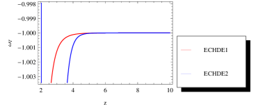
Figure 1: Plot of $\omega_{T}$ versus $z$. The curves of ECHDE model are characterize as red is for the first category (21), blue is for the second category (22).

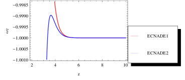
Figure 2: Plot of $\omega_{T}$ versus $z$. The curves of ECNADE model are characterize as red is for the first category (21), blue is for the second category (22).

VII Analysis of reconstructed model

In order to analysis the reconstructed models, we check in the section the behavior of certains physical parameters as speed of sound and the Statefinder parameters. Squared speed of sound,

$$v_{s}^{2}=\frac{\dot{p}_{eff}}{\dot{\rho}_{eff}},$$ (102)

is an important quantity to test the stability of the background evolution. The study of the stability of the model will depend on the sign of (102). Several discussions were conducted leading to interesting results setare3 ; kim ; jawad ; Chattopadhyay . We here considered the $v_{s}^{2}$ as equal to (102 and plot this $v_{s}^{2}$ verses the cosmic time $z$ for both reconstructions of $f(T)$ ECHDE and ECNADE models.

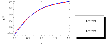
Figure 3: Plot of $v_{s}^{2}$ versus $z$. The curves of ECHDE model are characterize as red is for the first category (21), blue is for the second category (22).

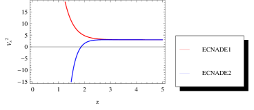
Figure 4: Plot of $v_{s}^{2}$ versus $z$. The curves of ECNADE model are characterize as red is for the first category (21), blue is for the second category (22).

From the figures4, we can observe the instability of ECHDE model for the two categories of scale factor $0<z<0.6$ but the ECHDE model is stable when $z>0.6$. The figure4 indicates that the second category of scale factor corresponding to ECNADE model is unstable for $0<z<2$ and stable when $z>2$. On the other hand, for the first category corresponding to the ECNADE model remains stable whatever the value of $z$.

VIII Statefinder parameters

A series of candidates for the Dark Energy model have been suggested till date and it is noted between them some problems of competitivity. In order to try to solve these problems, Sahni et al. varun1 introduced the statefinder $\{r,s\}$ diagnostic pair. This pair reads varun1 ; varun2

$$r=\frac{\dddot{a}}{H^{3}\,a},\quad s=\frac{r-1}{3\,\left(q-\frac{1}{2}\right)},$$ (103)

with $q$ and $H$, respectively the deceleration and Hubble parameters. Thus, we can determine geometrically properties of Dark Energy. Interesting results have been found there sharif ; Panotopoulos ; Chakraborty ; varun1 ; varun2 ; Zimdahl . We created the $\{r-s\}$ trajectories and compared with the $\Lambda$CDM limit based on the reconstructed models. We can observe from the figures6, 6 that although the trajectories approache the $\Lambda$CDM limit. Finally, the behavior of physical parameters as speed of sound and the Statefinder parameters are compatible with current observational data.

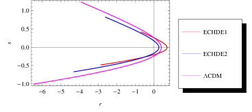
Figure 5: Plot of $\{r-s\}$. The curves of ECHDE model are characterize as red is for the first category (21), blue is for the second category (22).

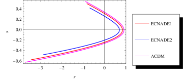
Figure 6: Plot of $\{r-s\}$. The curves of ECNADE model are characterize as red is for the first category (21), blue is for the second category (22).

IX Conclusions

In this paper, we investigated how the theory of modified gravity $f(T)$ where $T$ denotes the torsion scalar can describe the Entropy-Corrected holographic Dark Energy (ECHDE) and the Entropy-Corrected New Agegraphic Dark Energy (ECNADE) models. To achieve this, We have proceded to reconstruct the different algebraic function according to the HDE, ECHDE, NADE and ECNADE models by making use of of two categories of scale factors previously described. The EoS parameters have been determined and we note that for the first class of scale factor, the EoS parameters indicates to a accelerating expanded phantom-like universe, i.e. $\omega_{T}<-1$. We see from figures2,2 also that the EoS parameter $\omega_{T}$ according to the current observational data. On the other hand, for the second class of scale factor, We can note from figures2,2 that the EoS parameter satisfies $-1<\omega_{T}<-1/3$ which data indicates to a accelerating expanded quintessence-like universe. To ensure viability of the reconstructed models, we performed a stability analysis in In order to ensure viability of the reconstructed models, we performed a stability analysis by checking the behavior of certains physical parameters as speed of sound and the Statefinder parameters. From the figures4, we can observe the instability of ECHDE model for the two class of scale factor $0<z<0.6$ but the ECHDE model is stable when $z>0.6$. The figure4 indicates that the second category of scale factor from ECNADE model is unstable for $0<z<2$ and stable when $z>2$. On the other hand, for the first category of scale factor, the ECNADE model remains stable whatever the value of $z$. Finally, we have created the $\{r-s\}$ trajectories and compared with the $\Lambda$CDM limit. We can observe from the figures6, 6 that although the trajectories approache the $\Lambda$CDM limit. Finally, the behavior of physical parameters as speed of sound and the Statefinder parameters are compatible with current observational data.

References

• (1) S. Perlmutter et al. [SNCP Collaboration], Astrophys. J. 517, 565 (1999); A. G. Riess et al.[SNST Collaboration], Astron. J. 116, 1009 (1998).
• (2) D. N. Spergel et al. [WMAP Collaboration], Astrophys. J. Suppl. 148, 175 (2003); ibid. 170, 377 (2007); E. Komatsu et al. [WMAP Collaboration], ibid. 180, 330 (2009).
• (3) E. Komatsu et al. [WMAP Collaboration], Astrophys. J. Suppl. 192, 18 (2011).
• (4) M. Tegmark et al., Phys. Rev. D 69, 103501 (2004); U. Seljak et al. [SDSS Collaboration], Phys. Rev. D 71, 103515 (2005).
• (5) D. J. Eisenstein et al., Astrophys. J. 633, 560 (2005).
• (6) B. Jain and A. Taylor, Phys. Rev. Lett. 91, 141302 (2003).
• (7) T. Padmanabhan, Phys. Rep. 380, 235 (2003);
P.J.E. Peebles, B. Ratra, Rev. Mod. Phys. 75, 559 (2003).
• (8) E.J. Copeland, M. Sami, S. Tsujikawa, Int. J. Mod. Phys. D 15, 1753 (2006).
• (9) P. Horava, D. Minic, Phys. Rev. Lett. 85, 1610 (2000);
P. Horava, D. Minic, Phys. Rev. Lett. 509, 138 (2001);
S. Thomas, Phys. Rev. Lett. 89, 081301 (2002).
• (10) G. ’t Hooft, gr-qc/9310026;
L. Susskind, J. Math. Phys. 36, 6377 (1995).
• (11) W. Fischler, L. Susskind, hep-th/9806039.
• (12) A. Cohen, et al., Phys. Rev. Lett. 82, 4971 (1999).
• (13) M. Li, Phys. Lett. B 603, 1 (2004).
• (14) K. Enqvist, M.S. Sloth, Phys. Rev. Lett. 93, 221302 (2004);
Q.G. Huang, Y. Gong, JCAP 08, 006 (2004);
Q.G. Huang, M. Li, JCAP 08, 013 (2004);
Y. Gong, Phys. Rev. D 70, 064029 (2004).
• (15) E. Elizalde, S. Nojiri, S.D. Odintsov, P. Wang, Phys. Rev. D 71, 103504 (2005);
X. Zhang, F.Q. Wu, Phys. Rev. D 72, 043524 (2005);
B. Guberina, R. Horvat, H. Stefancic, JCAP 05, 001 (2005);
J.Y. Shen, B. Wang, E. Abdalla, R.K. Su, Phys. Lett. B 609, 200 (2005);
B. Wang, E. Abdalla, R.K. Su, Phys. Lett. B 611, 21 (2005).
• (16) J.P.B. Almeida, J.G. Pereira, Phys. Lett. B 636, 75 (2006);
B. Guberina, R. Horvat, H. Nikolic, Phys. Lett. B 636, 80 (2006);
H. Li, Z.K. Guo, Y.Z. Zhang, Int. J. Mod. Phys. D 15, 869 (2006);
X. Zhang, Phys. Rev. D 74, 103505 (2006);
X. Zhang, F.Q. Wu, Phys. Rev. D 76, 023502 (2007).
• (17) L. Xu, JCAP 09, 016 (2009);
M. Jamil, M.U. Farooq, M.A. Rashid, Eur. Phys. J. C 61, 471 (2009);
M. Jamil, M.U. Farooq, Int. J. Theor. Phys. 49, 42 (2010);
A. Sheykhi, Class. Quantum Grav. 27, 025007 (2010);
A. Sheykhi, Phys. Lett. B 682, 329 (2010).
• (18) K. Karami, JCAP 01, 015 (2010);
K. Karami, J. Fehri, Phys. Lett. B 684, 61 (2010);
• (19) R. Banerjee, B.R. Majhi, Phys. Lett. B 662, 62 (2008);
R. Banerjee, B.R. Majhi, JHEP 06, 095 (2008);
R. Banerjee, S.K. Modak, JHEP 05, 063 (2009);
B.R. Majhi, Phys. Rev. D 79, 044005 (2009);
S.K. Modak, Phys. Lett. B 671, 167 (2009);
M. Jamil, M.U. Farooq, JCAP 03, 001 (2010);
H.M. Sadjadi, M. Jamil, EPL, 92, 69001 (2010);
S.W. Wei, Y.X. Liu, Y.Q. Wang, H. Guo, arXiv:1002.1550;
D.A. Easson, P.H. Frampton, G.F. Smoot, arXiv:1003.1528.
• (20) H. Wei, Commun. Theor. Phys. 52, 743 (2009).
• (21) R.G. Cai, Phys. Lett. B 657, 228 (2007).
• (22) F. Karolyhazy, Nuovo. Cim. A 42, 390 (1966);
F. Karolyhazy, A. Frenkel, B. Lukacs, in Physics as natural Philosophy edited by A. Shimony, H. Feschbach, MIT Press, Cambridge, MA, (1982);
F. Karolyhazy, A. Frenkel, B. Lukacs, in Quantum Concepts in Space and Time edited by R. Penrose, C.J. Isham, Clarendon Press, Oxford, (1986).
• (23) M. Maziashvili, Int. J. Mod. Phys. D 16, 1531 (2007);
M. Maziashvili, Phys. Lett. B 652, 165 (2007).
• (24) H. Wei, R.G. Cai, Phys. Lett. B 660, 113 (2008).
• (25) H. Wei, R.G. Cai, Eur. Phys. J. C 59, 99 (2009).
• (26) Y.W. Kim, et al., Mod. Phys. Lett. A 23, 3049 (2008);
J.P. Wu, D.Z. Ma, Y. Ling, Phys. Lett. B 663, 152 (2008);
J. Zhang, X. Zhang, H. Liu, Eur. Phys. J. C 54, 303 (2008);
I.P. Neupane, Phys. Lett. B 673, 111 (2009);
A. Sheykhi, Phys. Rev. D 81, 023525 (2010).
• (27) K.Y. Kim, H.W. Lee, Y.S. Myung, Phys. Lett. B 660, 118 (2008).
• (28) A. Sheykhi, Phys. Lett. B 680, 113 (2009);
K. Karami, M.S. Khaledian, F. Felegary, Z. Azarmi, Phys. Lett. B 686, 216 (2010);
K. Karami, A. Abdolmaleki, Astrophys. Space Sci. 330, 133 (2010).
• (29) K. Karami, A. Sorouri, Phys. Scr. 82, 025901 (2010);
K. Karami, et al., Gen. Relativ. Gravit. 43, 27 (2011);
M.U. Farooq, M.A. Rashid, M. Jamil, Int. J. Theor. Phys. 49, 2278 (2010);
M. Malekjani, A. Khodam-Mohammadi, arXiv:1004.1017.
• (30) M. J. S. Houndjo, Int. J. Mod. Phys. D. 21, 1250003 (2012). arXiv: 1107.3887 [astro-ph.CO].
• (31) T. Harko, F. S. N. Lobo, S. Nojiri and S. D. Odintsov, Phys. Rev. D 84 (2011) 024020. [arXiv:1104.2669 [gr-qc]].
• (32) K. Bamba, C.-Q. Geng, S. Nojiri, S. D. Odintsov, arXiv:0909.4397.
• (33) M. J. S. Houndjo, M. E. Rodrigues, D. Momeni, R. Myrzakulov .arXiv:1301.4642 [gr-qc].
• (34) M.E. Rodrigues, M.J.S. Houndjo, D. Momeni, R. Myrzakulov, arXiv:1212.4488.
• (35) K. Bamba, S. D. Odintsov, L. Sebastiani, S. Zerbini, arXiv:0911.4390.
• (36) S. Nojiri, S. D. Odintsov, A. Toporensky, P. Tretyakov, arXiv:0912.2488.
• (37) J.Β AmorΓ³s, J.Β de Haro and S.Β D.Β Odintsov, β€œBouncing Loop Quantum Cosmology from $f(T)$ gravity,” Physical Review D 87, 104037 (2013) [arXiv:1305.2344 [gr-qc]]; K.Β Bamba, J.Β de Haro and S.Β D.Β Odintsov, β€œFuture Singularities and Teleparallelism in Loop Quantum Cosmology,” JCAP 1302 (2013) 008 [arXiv:1211.2968 [gr-qc]]; K.Β Bamba, S. ’i.Β Nojiri and S.Β D.Β Odintsov, β€œEffective $f(T)$ gravity from the higher-dimensional Kaluza-Klein and Randall-Sundrum theories,” arXiv:1304.6191 [gr-qc]; G. R. Bengochea, R. Ferraro and , Phys. Rev. D 79, 124019 (2009) [arXiv:0812.1205 [astro-ph]].
• (38) E. V. Linder, Phys.Rev. D 81, 127301 (2010) [Erratum-ibid. D 82, 109902 (2010)] [arXiv:1005.3039 [astro-ph.CO]].
• (39) K. Nozari, T. Azizi, Phys. Lett. B 680, 205 (2009).
• (40) S. Nojiri, S.D. Odintsov, Int. J. Geom. Meth. Mod. Phys. 4, 115 (2007).
• (41) H.M. Sadjadi, Phys. Rev. D 73, 063525 (2006).
• (42) M. Li, Phys. Lett. B 603, 1 (2004).
• (43) M. Li, X.D. Li, S. Wang, X. Zhang, JCAP 06, 036 (2009).
• (44) E.J. Copeland, M. Sami, S. Tsujikawa, Int. J. Mod. Phys. D 15, 1753 (2006).
• (45) Setare, M.R.: Phys. Lett. B 654 (2007) 1.
• (46) Kim, K.Y., Lee, H.W. and Myung, Y.S.: Phys. Lett. B 660 (2008) 118.
• (47) Jawad, A., Pasqua, A. and Chattopadhyay, S.: Astrophys. Space Sci. (2013, to appear).
• (48) Chattopadhyay, S. and Pasqua, A.: Astrophys. Space Sci. (2013, to appear).
• (49) Sharif, M. and Jawad, A.: Europ. Phys. J. C 72 (2012) 1901.
• (50) Panotopoulos, G.: Nuc. Phys. B 796 (2008) 66.
• (51) Chakraborty, S., Debnath, U., Jamil, M. and Myrzakulov, R.: Int. J. Theor. Phys. 51 (2012) 2246.
• (52) Sahni, V., Saini, T.D., Starobinsky, A.A. and Alam, U.: JETP Lett. 77 (2003) 201.
• (53) Sahni, V., Shafieloo, A. and Starobinsky, A.A.: Phys. Rev. D 78 (2008) 103502.
• (54) Zimdahl, W. and Pavon, D.: Gen. Rel. Grav. 36 (2004) 1483.
• (55) A. Starobinsky, JETP Lett. 86, 157 (2007).