Abstract

We consider a $(m+2)$-dimensional Einstein-Gauss-Bonnet model with the cosmological $\Lambda$-term. We restrict the metrics to be diagonal ones and find for certain $\Lambda=\Lambda(m)$ class of cosmological solutions with non-exponential time dependence of two scale factors of dimensions $m>2$ and $1$. Any solutions from this class describes an accelerated expansion of $m$-dimensional subspace and tends asymptotically to isotropic solution with exponental dependence of scale factors.

1 Introduction

In this paper we consider a $D$-dimensional gravitational model with Gauss-Bonnet term and cosmological term $\Lambda$, which extend the model with $\Lambda=0$ from ref. [1].

Earlier a wide class of exact cosmological solutions with diagonal metrics in this model with two and three different Hubble-like parameters, e.g. stable ones with exponential behaviour of scalar factors, were studied in numerous publications, see [2]-[17]. The main part of these solutions have constant Hubble-like parameters, some of solutions deal with the case $\Lambda=0$.

Recently in ref. [10] a systematic study of dynamical solutions in low dimensions with two non-constant Hubble-like parameters $H(t)$ and $h(t)$, corresponding to $3$- and $l$-dimensional factor spaces was started for $l=1,2$ ($l$ is dimension of the internal space) and arbitrary $\Lambda$. We note that in ref. [11] there is a continuation of this study for the case of general $l$.

Here we deal with a class of exact dynamical solutions with non-constant $H(t)$ and $h(t)$, which correspond to $m$-dimensional ($m>2$ ) and one-dimensional factor spaces, when some fine-tuned $\Lambda=\Lambda(m)$ is chosen. The solution describes an accelerated expansion of $m$-dimensional subspace.

The structure of the paper is as follows. In Section 2 we present a setup. A class of exact cosmological solutions with diagonal metrics is found for certain $\Lambda$ in Section 3. In Section 4 we consider examples of solutions for $m=3,4,5$.

2 The set up

The action of the model reads

$$S=\int_{M}d^{D}z\sqrt{|g|}\{\alpha_{1}(R[g]-2\Lambda)+\alpha_{2}{\cal L}_{2}[g]\},$$ (2.1)

where $g=g_{MN}dz^{M}\otimes dz^{N}$ is the metric defined on the manifold $M$, ${\dim M}=D$, $|g|=|\det(g_{MN})|$, $\Lambda$ is the cosmological term, $R[g]$ is scalar curvature,

$${\cal L}_{2}[g]=R_{MNPQ}R^{MNPQ}-4R_{MN}R^{MN}+R^{2}$$

is the standard Gauss-Bonnet term and $\alpha_{1}$, $\alpha_{2}$ are nonzero constants.

We consider the manifold

$$M={\mathbb{R}}\times M_{1}\times\ldots\times M_{n}$$ (2.2)

with the metric

$$g=-dt\otimes dt+\sum_{i=1}^{n}e^{2\beta^{i}(t)}dy^{i}\otimes dy^{i}.$$ (2.3)

We have the set of equations [12]

$$E=G_{ij}h^{i}h^{j}+2\Lambda-\alpha G_{ijkl}h^{i}h^{j}h^{k}h^{l}=0,$$ (2.4)

$$Y_{i}=\frac{dL_{i}}{dt}+(\sum_{j=1}^{n}h^{j})L_{i}-\frac{2}{3}(G_{sj}h^{s}h^{j}-4\Lambda)=0,$$ (2.5)

where $h^{i}=\dot{\beta}^{i}$,

$$L_{i}=L_{i}(h)=2G_{ij}h^{j}-\frac{4}{3}\alpha G_{ijkl}h^{j}h^{k}h^{l},$$ (2.6)

$i=1,\ldots,n$, where $\alpha=\alpha_{2}/\alpha_{1}$. Here

$$G_{ij}=\delta_{ij}-1,\qquad G_{ijkl}=G_{ij}G_{ik}G_{il}G_{jk}G_{jl}G_{kl}$$ (2.7)

are, respectively, the components of two metrics on ${\mathbb{R}}^{n}$ [4, 5]. The first one is a 2-metric and the second one is a Finslerian 4-metric. For $n>3$ we get a set of forth-order polynomial equations.

Here we present a class of solutions to the set of equations (2.4), (2.5) of the following form

$$(h^{i}(t))=(\overbrace{H(t),\ldots,H(t)}^{m},h(t)).$$ (2.8)

where $H(t)$ is the Hubble-like parameter corresponding to $m$-dimensional factor space with $m>2$, and $h(t)$ is the Hubble-like parameter corresponding to one-dimensional factor space.

We put

$$H(t)>0,\qquad H^{2}+\dot{H}>0,$$ (2.9)

where $t>0$, for a possible description of an accelerated expansion of a $3$-dimensional subspace (which may describe our Universe) in our epoch ($t_{0}>0$ [18, 19].

Here we put $\alpha<0$. The dynamical equation (2.5) for $H$ has the following form

$$\begin{gathered}3(m-1)\dot{H}+3\dot{h}+2\alpha(m-1)(m-2)(2((m-3)H+3h)H\dot{H}+((m-3)\dot{H}+3\dot{h})H^{2})\\ +2\alpha m(m-1)(m-2)(m-3)H^{4}+2\alpha(m-1)(m-2)(4m-3)hH^{3}\\ +2(m-1)((1+3\alpha h^{2})m-6\alpha H^{2})H^{2}+(4m-3)hH+3h^{2}=4\Lambda\end{gathered}$$ (2.10)

The dynamical equation corresponding to $h$ reads as follows

$$\begin{gathered}3m\dot{H}+6\alpha m(m-1)(m-2)H^{2}\dot{H}+2\alpha m^{2}(m-1)(m-2)H^{4}\\ +2\alpha m(m-1)(m-2)hH^{3}+m(2m+1)H^{2}+mhH=4\Lambda\end{gathered}$$ (2.11)

The equation (2.4) may be written the following form:

$$\begin{gathered}\alpha m(m-1)(m-2)(m-3)H^{4}+4\alpha m(m-1)(m-2)hH^{3}\\ +m(m-1)H^{2}+2mhH=2\Lambda\end{gathered}$$ (2.12)

The relation (2.12) is solvable with respect to h and we obtain the following expression

$$h=-\frac{1}{2}\frac{\alpha m(m-1)(m-2)(m-3)H^{4}+m(m-1)H^{2}-2\Lambda}{m\Biggl{(}2\alpha(m-1)(m-2)H^{2}+1\Biggr{)}H}$$ (2.13)

and then substituting this value of h into Eqs. (2.10) and (2.11). We obtain the relation for $\dot{H}$:

$$\dot{H}=-\frac{1}{2}\frac{\alpha m(m-1)(m-2)(m+1)H^{4}+m(m+1)H^{2}-2\Lambda}{m\Biggl{(}2\alpha(m-1)(m-2)H^{2}+1\Biggr{)}}$$ (2.14)

and from the formula (2.10) it is possible to obtain the relation for $\dot{h}$ :

$$\begin{gathered}\dot{h}=\frac{1}{4}\frac{1}{m^{2}(2\alpha(m-1)(m-2)H^{2}+1)^{3}H^{2}}\times\\ \times\Biggl{[}2\alpha^{3}m^{2}(m+1)(m-3)(m-1)^{3}(m-2)^{3}H^{10}\\ +\alpha^{2}m^{2}(m+1)(3m-13)(m-1)^{2}(m-2)^{2}H^{8}\\ +2\alpha m(m-1)(m-2)\Biggl{(}(1+4\alpha\Lambda)m^{3}-3m^{2}-4(1+7\alpha\Lambda)m+24\alpha\Lambda\Biggr{)}H^{6}\\ +m(m-1)\Biggl{(}(1+12\alpha\Lambda)m^{2}+(1+4\alpha\Lambda)m-56\alpha\Lambda\Biggr{)}H^{4}\\ -4\Lambda\Biggl{(}6\alpha\Lambda m^{2}-(1+18\alpha\Lambda)m+12\alpha\Lambda\Biggr{)}H^{2}-4\Lambda^{2}\Biggr{]}.\end{gathered}$$ (2.15)

3 Exact solutions

Now we consider special solution to equations from the previous section. As it can be seen from the expressions (2.14) and (2.15), the problem of finding a general integral in an analytical form from the above expressions causes enormous difficulties, i.e. the total integral can be calculated only by numerical methods with varying degrees of accuracy. But in the case when $\alpha=-1$

$$\Lambda=\frac{1}{8}\frac{m(m+1)}{(m-1)(m-2)}$$ (3.1)

these expressions are greatly simplified and, by calculating the integrals, one can find such dynamic exact solutions as $H(t)$ and $h(t)$. We already know that in this value of $\Lambda$ we obtain a solution with zero variation of $G$ [15]. By substituting these values of $\alpha$ and $\Lambda$ into (2.14) and (2.15) we obtain

$$\dot{H}=\frac{1}{8}\frac{(m+1)\Biggl{(}1-2(m-1)(m-2)H^{2}\Biggr{)}}{(m-1)(m-2)}$$ (3.2)

and

$$\dot{h}=\frac{(m+1)}{64}\times\qquad\qquad\qquad$$ (3.3)

$$\frac{\Biggl{(}4(m-3)(m-1)^{2}(m-2)^{2}H^{4}+8(m-1)(m-2)H^{2}-(m+1)\Biggr{)}}{(m-1)^{2}(m-2)^{2}H^{2}}$$

Then, we calculate the integral of (3.2) with the help of a tabular integral and taking into account the initial condition $H(0)=0$, we find the following formulas for H for arbitrary m.

$$H=\frac{4b}{m+1}th(bt)$$ (3.4)

where

$$b=\frac{m+1}{4\sqrt{2(m-1)(m-2)}}$$ (3.5)

Now we find the expression $\frac{dh}{dH}$ with the help of equations (3.2) and (3.3):

$$\frac{dh}{dH}=-\frac{1}{8}\Biggl{(}2(m-3)+\frac{(m+1)}{(m-1)(m-2)H^{2}}\Biggr{)}$$ (3.6)

From the last equation, we compute the integral and taking into account the initial condition $H(0)=0$, we find the following formulas for h for arbitrary m.

$$h=\frac{1}{8}\Biggl{(}\frac{(m+1)}{(m-1)(m-2)H}-2(m-3)H\Biggr{)}$$ (3.7)

, i.e.

$$h=b\Biggl{(}cth(bt)-\frac{m-3}{m+1}th(bt)\Biggr{)}$$ (3.8)

As it can be seen from the formulas (3.4) and (3.8), as $t\to\infty$, the parameters $H(t)$ and $h(t)$ approach to the same value $H_{st}=(2(m-1)(m-2))^{-\frac{1}{2}}$ , i.e., anisotropic solution for Hubble-like parameters turns to static isotropic solution from ref. [13] with critical value of $\Lambda$.

Accelerated expansion.

The differencial equations $\frac{d\beta^{i}}{dt}=h^{i}$, $i=1,\dots,m+1$ could be readily integrated. We get for $t>0$

$$\beta^{i}(t)=\frac{4}{m+1}\ln(ch(bt))+\beta^{i}_{0},$$ (3.9)

where $\beta^{i}_{0}$ are constants, $i=1,\dots,m$, and

$$\beta^{m+1}(t)=\ln(sh(bt))-\frac{m-3}{m+1}\ln(ch(bt))+\beta^{m+1}_{0},$$ (3.10)

and $\beta^{m+1}_{0}$ is constant

For scale factors we find

$$a_{i}\left(t\right)=e^{\beta^{i}}=a_{i0}\Biggl{(}ch\left(bt\right)\Biggr{)}^{\frac{4}{m+1}},$$ (3.11)

$i=1,\dots,m$ and

$$a_{m+1}\left(t\right)=e^{\beta^{m+1}}=a_{m+1,0}(sh\left(bt\right)\Biggl{(}ch\left(bt\right)\Biggr{)}^{\frac{3-m}{m+1}}.$$ (3.12)

The positive constants $a_{i0}=e^{\beta^{i}_{0}}$ and $a_{m+1,0}=e^{\beta^{m+1}_{0}}$ may be restricted by isotropy condition for our $3d$ Universe: $a_{i0}=a_{0}$, $i=1,2,3$.

We obtain

$$\frac{da_{i}\left(t\right)}{dt}=a_{0}\frac{4b}{m+1}\Biggl{(}ch\left(bt\right)\Biggr{)}^{\frac{3-m}{m+1}}sh(bt),$$ (3.13)

and

$$\frac{d^{2}}{d^{2}t}a_{i}\left(t\right)=a_{0}\frac{4b^{2}}{m+1}\Biggl{(}ch\left(bt\right)\Biggr{)}^{\frac{2(1-m)}{m+1}}\Biggl{[}ch^{2}(bt)+\frac{3-m}{m+1}sh^{2}\left(bt\right)\Biggr{]},$$ (3.14)

$i=1,2,3$.

It may be readily verified that the inequality $d^{2}a_{i}/d^{2}t>0$ is obeyed for all values of $t>0$.

Non-singular begaviour. We note that in the limit $t\to+0$ we get $a_{i}(t)\to a_{i0}$, $i=1,\dots,m$, and $a_{m+1}\sim t^{2}$, that is a Milne-type behaviour of scalar factors. It seems that our solution is a non-singular one with a horizon at $t=+0$ and a so-called “black universe” under horizon [20]. But this may be a subject of a separate research.

4 Examples

Here we consider three special solutions for $m=3,4,5.$

4.1 The case $m=3$

Let us consider the case $m=3$, which is a special one since in this case the internal space is isotropic. We get

$$\Lambda=\frac{3}{4}$$ (4.1)

and from (3.4) and (3.8) we obtain

$$H=\frac{1}{2}th(t),\qquad h=\frac{1}{2}cth(t)$$ (4.2)

and $b=1$.

The graphical representation of the functions $H$ and $h$ are shown in Fig. 1.

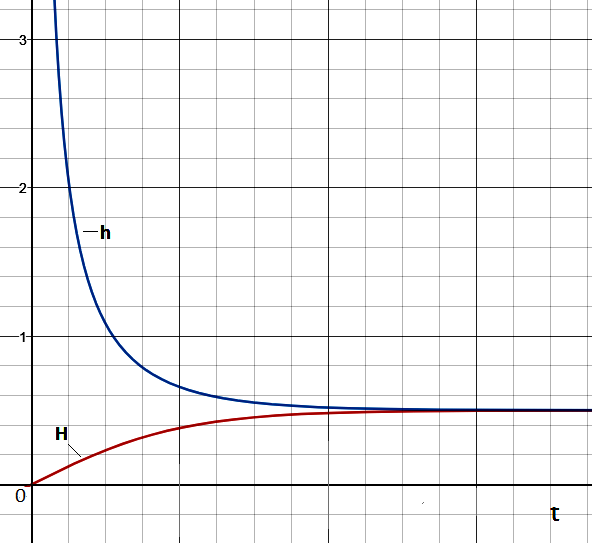
Figure 1: Time evolution of the Hubble-like parameters $H$ and $h$ in the case $m=3$ and $\Lambda=\frac{3}{4}$

Here our solution has an attractor (isotropic) static solution for $t\to+\infty$, i.e. $H(t)\to H_{st}=\frac{1}{2}$ and $h(t)\to h_{st}=\frac{1}{2}$.

4.2 The case $m=4$

Now we consider the case $m=4$. We obtain

$$\Lambda=\frac{5}{12},$$ (4.3)

$$H=\frac{1}{\sqrt{12}}th(bt)$$ (4.4)

and

$$h=\frac{5}{4\sqrt{12}}\Biggl{(}cth(bt)-\frac{1}{5}th(bt)\Biggr{)},$$ (4.5)

where $b=\frac{5}{4\sqrt{12}}$.

4.3 The case $m=5$

In the case $m=5$ we get

$$\Lambda=\frac{5}{16},$$ (4.6)

,

$$H=\frac{1}{\sqrt{24}}th(bt)$$ (4.7)

and

$$h=\frac{1}{2\sqrt{24}}\Biggl{(}3cth(bt)-th(bt)\Biggr{)},$$ (4.8)

where $b=\frac{3}{2\sqrt{24}}$.

Here we get $H(t)\to H_{st}=\frac{1}{\sqrt{24}}$ and $h(t)\to h_{st}=\frac{1}{\sqrt{24}}$, as $t\to+\infty$.

5 Conclusions

We have considered the $D$-dimensional Einstein-Gauss-Bonnet (EGB) model with the $\Lambda$-term and two constants $\alpha_{1}$ and $\alpha_{2}$. By using the ansatz with diagonal cosmological metrics, we have found for $D=m+2$, $\alpha=\alpha_{2}/\alpha_{1}=-1$ and certain $\Lambda=\Lambda(m)$ a class of solutions with non-exponential time dependence of $2$ scale factors, governed by two Hubble-like parameters $H(t)>0$, $h(t)$, corresponding to submanifolds of dimensions $m>2$ and $1$, respectively.

For any $m>2$ the Hubble-like parameters have asymptotically isotropic limits $H(t)\to H_{st}>0$, $h(t)\to h_{st}=H_{st}$, which corresponds to critical isotropic exponential solutions from ref. [13]. For any $m>2$ we have obtained an accelerated expansion of $m$-dimensional subspace.

Acknowledgments This work was supported in part by the Russian Foundation for Basic Research grant No. 16-02-00602 and by the Ministry of Education of the Russian Federation (the Agreement number 02.a03.21.0008 of 24 June 2016).

References

• [1] N. Deruelle, On the approach to the cosmological singularity in quadratic theories of gravity: the Kasner regimes, Nucl. Phys. B 327, 253-266 (1989).
• [2] E. Elizalde, A.N. Makarenko, V.V. Obukhov, K.E. Osetrin and A.E. Filippov, Stationary vs. singular points in an accelerating FRW cosmology derived from six-dimensional Einstein-Gauss-Bonnet gravity, Phys. Lett. B 644, 1-6 (2007); hep-th/0611213.
• [3] S.A. Pavluchenko, On the general features of Bianchi-I cosmological models in Lovelock gravity, Phys. Rev. D 80, 107501 (2009); arXiv: 0906.0141.
• [4] V.D. Ivashchuk, On anisotropic Gauss-Bonnet cosmologies in (n + 1) dimensions, governed by an n-dimensional Finslerian 4-metric, Grav. Cosmol. 16(2), 118-125 (2010); arXiv: 0909.5462.
• [5] V.D. Ivashchuk, On cosmological-type solutions in multidimensional model with Gauss-Bonnet term, Int. J. Geom. Meth. Mod. Phys. 7(5), 797-819 (2010); arXiv: 0910.3426.
• [6] D. Chirkov, S. Pavluchenko and A. Toporensky, Exact exponential solutions in Einstein-Gauss-Bonnet flat anisotropic cosmology, Mod. Phys. Lett. A 29, 1450093 (11 pages) (2014); arXiv:1401.2962.
• [7] D. Chirkov, S.A. Pavluchenko and A. Toporensky, Non-constant volume exponential solutions in higher-dimensional Lovelock cosmologies, Gen. Relativ. Gravit. 47: 137 (33 pages) (2015); arXiv: 1501.04360.
• [8] V.D. Ivashchuk and A.A. Kobtsev, On exponential cosmological type solutions in the model with Gauss-Bonnet term and variation of gravitational constant, Eur. Phys. J. C 75: 177 (12 pages) (2015); arXiv:1503.00860.
• [9] S.A. Pavluchenko, Stability analysis of exponential solutions in Lovelock cosmologies, Phys. Rev. D 92, 104017 (2015); arXiv: 1507.01871.
• [10] S.A. Pavluchenko, Cosmological dynamics of spatially flat Einstein-Gauss-Bonnet models in various dimensions: Low-dimensional $\Lambda$-term case, Phys. Rev. D 94, 084019 (2016); arXiv: 1607.07347.
• [11] S.A. Pavluchenko, Cosmological dynamics of spatially flat Einstein-Gauss-Bonnet models in various dimensions: High-dimensional $\Lambda$-term case, Eur. Phys. J. C 77, 503 (2017); arXiv: 1705.02578.
• [12] K.K. Ernazarov, V.D. Ivashchuk and A.A. Kobtsev, On exponential solutions in the Einstein-Gauss-Bonnet cosmology, stability and variation of G, Grav. Cosmol., 22 (3), 245-250 (2016).
• [13] V.D. Ivashchuk, On stability of exponential cosmological solutions with non-static volume factor in the Einstein-Gauss-Bonnet model, Eur. Phys. J. C 76 431 (2016); arXiv: 1607.01244v2.
• [14] V.D. Ivashchuk, On Stable Exponential Solutions in Einstein-Gauss-Bonnet Cosmology with Zero Variation of G, Grav. Cosmol., 22 (4), 329-332 (2016); see corrected version in arXiv: 1612.07178.
• [15] K.K. Ernazarov and V.D. Ivashchuk, Stable exponential cosmological solutions with zero variation of G in the Einstein-Gauss-Bonnet model with a $\Lambda$-term, Eur. Phys. J. C 77 89 (2017); arXiv: 1612.08451.
• [16] K.K. Ernazarov, V.D. Ivashchuk, Stable exponential cosmological solutions with zero variation of G and three different Hubble-like parameters in the Einstein-Gauss-Bonnet model with a $\Lambda$-term, Eur. Phys. J. C (2017) 77: 402 (7 pages); arXiv:1705.05456.
• [17] D.M. Chirkov and A.V. Toporensky, On stable exponential cosmological solutions in the EGB model with a $\Lambda$-term in dimensions $D=5,6,7,8$; arXiv:1706.08889.
• [18] A.G. Riess et al. Observational evidence from supernovae for an accelerating universe and a cosmological constant, Astron. J. 116, 1009-1038 (1998).
• [19] S. Perlmutter et al. Measurements of Omega and Lambda from 42 High-Redshift Supernovae. Astrophys. J. 517, 565-586 (1999).
• [20] K.A. Bronnikov, H. Dehnen, V.N. Melnikov, Regular black holes and black universes, Gen. Rel. Grav. 39, 973-987 (2007); gr-qc/0611022.