Component-wise Approximate Bayesian Computation via Gibbs-like steps

Abstract

Approximate Bayesian computation methods are useful for generative models with intractable likelihoods. These methods are however sensitive to the dimension of the parameter space, requiring exponentially increasing resources as this dimension grows. To tackle this difficulty, we explore a Gibbs version of the Approximate Bayesian computation approach that runs component-wise approximate Bayesian computation steps aimed at the corresponding conditional posterior distributions, and based on summary statistics of reduced dimensions. While lacking the standard justifications for the Gibbs sampler, the resulting Markov chain is shown to converge in distribution under some partial independence conditions. The associated stationary distribution can further be shown to be close to the true posterior distribution and some hierarchical versions of the proposed mechanism enjoy a closed form limiting distribution. Experiments also demonstrate the gain in efficiency brought by the Gibbs version over the standard solution.

1 Introduction

Approximation Bayesian computation (ABC) is a computational method which stemmed from population genetics to deal with intractable likelihoods, that is models whose likelihood cannot be (easily) computed but which can be simulated from (Tavaré et al., 1997; Beaumont et al., 2002). Since then, it has been applied to numerous other fields: see for example Toni et al. (2008); Csilléry et al. (2010); Moores et al. (2015); Sisson et al. (2018). The principle of the method is to simulate pairs of parameters and pseudo-data from the prior predictive, keeping only the parameters that bring the pseudo-data close enough (within a pseudo-distance $\varepsilon$) to the observed data. Proximity is often defined in terms of a projection of the data, called a summary statistic. In general, practitioners of ABC aim to use informative summary statistics and select $\varepsilon$ to be as small as possible, since this leads to a higher-quality approximation. From the start, this method has suffered from the curse of dimensionality in that the dimension of the parameter to be inferred imposes a lower bound on the dimension of the corresponding summary statistic to be used (results by Fearnhead & Prangle (2012) and Li & Fearnhead (2018b) imply that the dimension of the summary statistic should be identical to the dimension of the parameter). This constraint impacts the range of the distance between observed and simulated summaries, with the distance choice having a growing impact as the dimension increases. Reducing the dimension of the summary is thus impossible without reducing the dimension of the parameter, which sounds an impossible goal unless one infers about one parameter at a time, suggesting a Gibbs sampling strategy where a different and much reduced dimension summary statistic is used for each component of the parameter. The purpose of this paper is to explore and validate this strategy, producing sufficient conditions for the convergence of the resulting algorithms.

Additionally, the Gibbs perspective allows us to account for the current values of the other components of the parameter and therefore to shy away from simulating from the prior which is an inefficient proposal. This feature connects this proposal with earlier solutions in the literature such as the Metropolis version of Marjoram et al. (2003) and the various sequential Monte Carlo schemes (Toni et al., 2008; Beaumont et al., 2009). There have been earlier ABC versions with Gibbs features, including Wilkinson et al. (2011), where a two-stage ABC-within-Gibbs algorithm is proposed towards bypassing the intractibility of one of the conditional distributions used in their Gibbs sampler. Since the other conditional distribution is simulated exactly, there is no convergence issue with this version. Note also that the summary statistics used in that paper are not chosen for dimension reduction purposes. Kousathanas et al. (2016) also run a Gibbs-like ABC algorithm that assumes the availability of conditionally sufficient statistics to preserve the coherence of the algorithm. Rodrigues et al. (2020) propose another Gibbs-like ABC algorithm in which the conditional distributions are approximated by regression models.

A Gibbs version of the ABC method offers a range of potential improvements compared with earlier versions, induced in most cases by the dimension reduction thus achieved. First, in hierarchical models, conditioning decreases the number of dependent components, and some of the conditionals may be available in closed form, which makes the approach only semi-approximate. Second, since the conditional targets live in spaces of low dimension, they can more easily be parametrised by low dimension functions of the conditioning terms. This justifies using a restricted range of collection of statistics, which may in addition depend on other parameters. Third, reducing the dimension of the summary statistic improves the approximation since a smaller tolerance can then be handled at a manageable computing cost.

This heuristic leads us to propose in Section 2 a generic algorithm called ABC-Gibbs. To show the theoretical validity of this idea, we successively show that, under some conditions:

1. for all $\varepsilon>0$, our ABC-Gibbs converges to a certain limiting distribution $\nu_{\varepsilon}$ in total variation distance,

2. when $\varepsilon\rightarrow 0$, $\|\nu_{\varepsilon}-\nu_{0}\|_{TV}\rightarrow 0$, with $\nu_{0}$ a distribution,

3. $\nu_{0}$ is the limiting distribution of Vanilla ABC with tolerance $\varepsilon$ set to $0$.

The first result corresponds to Theorem 2.1 in the general case; Theorem 11.1 states this result for hierarchical models under looser assumptions. The second result is a consequence of Theorem 2.3. The last result follows from the results of Section 6.

2 Approximate Bayesian Gibbs sampling

2.1 Vanilla approximate Bayesian computation

Approximate Bayesian computation methods, summarised in Algorithm 1, provide a technique to sample posterior distributions when the corresponding likelihood $f(x|{\theta})$ is intractable, that is the numerical value $f(x|{\theta})$ cannot be computed in a reasonable amount of time, but the model is generative, that is it allows for the generation of synthetic data given a value of the parameter. Given a prior distribution on the parameter ${\theta}$, it builds upon samples from the associated prior predictive $({\theta}^{(i)},x^{(i)})_{i=1,\ldots,N}$ by selecting pairs such that the pseudo-data $x^{(i)}$ stand in a neighbourhood of the observed data $x^{\star}$.

Since both the simulated and observed dataset may belong to a space of a high dimension, the neighbourhood is usually defined with respect to a summary statistic $s(\cdot)$ of a lesser dimension and an associated distance $d$ (see Marin et al., 2012 for a review). Fearnhead & Prangle (2012) show that the optimal statistic is of the same dimension as the parameter ${\theta}$; in practice, the choice of $s$ remains a crucial issue.

Input: observed dataset $x^{\star}$, number of iterations $N$, threshold $\varepsilon>0$, summary statistic $s$.

Output: a sample $({\theta}^{(1)},\ldots,{\theta}^{(N)})$.

for $i=1,\dots,N$ do

       repeat

      ${\theta}^{(i)}\sim\pi(\cdot)$

      $x^{(i)}\sim f(\cdot\mid{\theta}^{(i)})$

      until $d\{s(x^{(i)}),s(x^{\star})\}<\varepsilon$

Algorithm 1 Vanilla Approximate Bayesian computation

The output of Algorithm 1 is a sample distributed from an approximation of the posterior (Tavaré et al., 1997; Sisson et al., 2018). Its density is written, with a notation coherent with the next sections:

$$\pi_{\varepsilon}\{{\theta}\mid s(x^{\star})\}\propto\int\pi({\theta})f(x\mid{\theta})\mathbf{1}_{d\{s(x),s(x^{\star})\}<\varepsilon}\,\mathrm{d}x.$$

This approximation depends on the choice of both the summary statistic $s$ and the tolerance level $\varepsilon$. Frazier et al. (2018) show its consistency, namely that when the number of observations tends to $\infty$ and the tolerance tends to $0$ at a proper relative rate, the approximate posterior concentrates at the true value of the parameter, albeit as a posterior distribution associated with the statistic $s$, rather than the true posterior, when $s$ is not sufficient. The shape of the asymptotic distribution is further discussed in Li & Fearnhead (2018b) and Frazier et al. (2018).

More to the point, given a fixed number of observations, the approximate posterior also converges to the posterior $\pi\{{\theta}\mid s(x^{\star})\}$, rather than to the standard posterior $\pi({\theta}\mid x^{\star})$, when the tolerance level goes to $0$. In practice, however, the tolerance level cannot be equal to zero and is customarily chosen as a simulated distance quantile (Sisson et al., 2018). In practice, a large sample of pseudo-observations is generated from the prior predictive and the corresponding distances to the observations are computed. We use the term reference table for this collection of parameters and distances. The tolerance is then derived as a small quantile of these distances.

2.2 Gibbs sampler

The Gibbs sampler, first introduced by Geman & Geman (1984) and generalised by Gelfand & Smith (1990), is an essential element in Markov chain Monte Carlo methods (Robert & Casella, 2004; Gelman et al., 2013). As described in Algorithm 2, for a parameter ${\theta}=(\theta_{1},\dots,\theta_{n})$, it produces a Markov chain associated with a given target joint distribution, denoted $\pi$, by alternatively sampling from each of its conditionals.

Input: number of iterations $N$, starting point ${\theta}^{(0)}=(\theta^{(0)}_{1},\dots,\theta^{(0)}_{n})$.

Output: a sample $({\theta}^{(1)},\dots,{\theta}^{(N)})$.

for $i=1,\ldots,N$ do

       for $j=1,\ldots,n$ do

             $\theta_{j}^{(i)}\sim\pi(\cdot\mid\theta_{1}^{(i)},\ldots,\theta_{j-1}^{(i)},\theta_{j+1}^{(i-1)},\ldots,\theta_{n}^{(i-1)})$

Algorithm 2 Gibbs sampler

Gibbs sampling is well suited to high-dimensional situations where the conditional distributions are easy to sample. In particular, as illustrated by the long-lasting success of the BUGS software (Lunn et al., 2010), hierarchical Bayes models often allow for simplified conditional distributions thanks to partial independence properties. Considering for instance the common hierarchical model (Lindley & Smith, 1972; Carlin & Louis, 1996) defined by

$$x_{j}\mid\mu_{j}\sim\pi(x_{j}\mid\mu_{j})\,,\qquad\mu_{j}\mid\alpha\stackrel{{\scriptstyle\text{i.i.d.}}}{{\sim}}\pi(\mu_{j}\mid\alpha)\,,\qquad\alpha\sim\pi(\alpha)\,.$$ (1)

The joint posterior of $\mu=(\mu_{1},\dots,\mu_{n})$ conditional on $\alpha$ then factorises as

$$\pi(\mu\mid x_{1},\dots,x_{n},\alpha)\propto\prod_{j=1}^{n}\pi(\mu_{j}\mid\alpha)\pi(x_{j}\mid\mu_{j}).$$

This implies that the full conditional posterior of a given $\mu_{j}$ only depends on $\alpha$ and $x_{j}$, independently of the other $(\mu_{\ell},x_{\ell})$’s.

2.3 Component-wise Approximate Bayesian Computation

When handling a model such as (1) with both a high-dimensional parameter and an intractable likelihood, the Gibbs sampler cannot be implemented, while the vanilla ABC sampler is highly inefficient. This curse of dimensionality attached to the ABC algorithm is well documented (Li & Fearnhead, 2018b).

Bringing both approaches together may subdue this loss efficiency, by sequentially sampling from the ABC version of the conditionals, whose density

$\pi_{\varepsilon_{j}}(\cdot\mid s_{j}(x^{\star},\theta^{(i)}_{1},\dots,\theta^{(i)}_{j-1},\theta^{(i-1)}_{j+1},\dots,\theta^{(i-1)}_{n}))$ is proportional (see (2.1)) to

$$\int\pi(\theta_{j}\mid\theta^{(i)}_{1},\dots,\theta^{(i)}_{j-1},\theta^{(i-1)}_{j+1},\dots,\theta^{(i-1)}_{n})f(x\mid\theta^{(i)}_{1},\dots,\theta^{(i)}_{j-1},\theta_{j},\theta^{(i-1)}_{j+1},\dots,\theta^{(i-1)}_{n})\mathbf{1}_{d\{s_{j}(x),s_{j}(x^{\star})\}<\varepsilon_{j}}\,\text{d}x\,.$$

Each step in Algorithm 2 is then replaced by a call to Algorithm 1, conditional on the other components of the parameter. We obtain a generic componentwise approximate Bayesian computational method, summarised as Algorithm 3.

This algorithm can be analysed as a variation of Algorithm 1 in which the synthetic data $x^{(i)}$ are simulated from the conditional posterior predictive, rather than from the prior predictive. This may result in simulating both parameters and pseudo-data component-wise from spaces of smaller dimension. This also allows the use of statistics of lower dimension, as exemplified in Section 5.

Each stage $j$ of the algorithm now requires its own tolerance level $\varepsilon_{j}$ and statistic $s_{j}$. This statistic can be a function of the observations, but also of the other parameters $(\theta_{i})_{i\neq j}$ which are conditioned upon at stage $j$. Typically, $\theta_{j}$ is of dimension 1 and so $s_{j}$ should also be of dimension 1, per the results of Fearnhead & Prangle (2012). Finding a good unidimensional statistic for each $\theta_{j}$ in ABC-Gibbs may prove easier than finding a good high-dimension statistic for Vanilla ABC.

Input: number of iterations $N$, starting point ${\theta}^{(0)}=(\theta^{(0)}_{1},\dots,\theta^{(0)}_{n})$, thresholds $\varepsilon=(\varepsilon_{1},\dots,\varepsilon_{n})$, statistics $s_{1},\dots,s_{n}$, distances on the statistics $d_{1},\dots,d_{n}$.

Output: a sample $({\theta}^{(1)},\ldots,{\theta}^{(N)})$.

for $i=1,\dots,N$ do

       for $j=1,\dots,n$ do

             $\theta^{(i)}_{j}\sim\pi_{\varepsilon_{j}}\{\cdot\mid s_{j}(x^{\star},\theta^{(i)}_{1},\dots,\theta^{i}_{j-1},\theta^{(i-1)}_{j+1},\dots,\theta^{(i-1)}_{n})\}$

Algorithm 3 ABC-Gibbs

If $\varepsilon_{j}=0$ and if $s_{j}$ is a conditionally sufficient statistic, the corresponding $j$th step in Algorithm 3 is an exact simulation from the corresponding conditional. In particular, if some of the conditional distributions can be perfectly simulated, this cancels the need for an approximate step in the algorithm. In practice, to simulate from the approximate conditional, and similarly to Algorithm 1, we take $\varepsilon_{j}$ as an empirical distance quantile. In other words, for the $j$th component of the parameter, conditional on the other components, we simulate a small reference table from its conditional prior and output the parameter associated with the smallest distance.

At first, the purpose of this algorithm may sound unclear as the limiting distribution and its existence are unknown. As shown in Theorem 2.1, convergence can indeed be achieved, based on a simple condition. For simplicity’s sake, we initially only consider the case when $n=2$ in Algorithm 3.

Theorem 2.1.

Assume that there exists $0<\kappa<1/2$ such that

$$\sup_{\theta_{1},\tilde{\theta}_{1}}\|\pi_{\varepsilon_{2}}[\cdot\mid s_{2}(x^{\star},\theta_{1}])-\pi_{\varepsilon_{2}}\{\cdot\mid s_{2}(x^{\star},\tilde{\theta}_{1})\}\|_{TV}=\kappa.$$

The Markov chain produced by Algorithm 3 then converges geometrically in total variation distance to a stationary distribution $\nu_{\varepsilon}$, with geometric rate $1-2\kappa$.

The proof of Theorem 2.1 is provided in the Supplementary Material, Section 11.2 and is based on a coupling argument.

The above assumption is satisfied in particular when the parameter space is compact. Possible relaxations are not covered in this paper. This theorem suffers from its generality, as the most practical situation in which the conditions are satisfied is obtained if all the parameters live in a compact space. However we can refine the previous result for many graphical models; such refinements are explored in the next sections.

We can extend the convergence result of Theorem 2.1 to the general case $n>2$:

Theorem 2.2.

Assume that for all $\ell\leq n$

$$\kappa_{\ell}=\sup_{{\theta}_{>\ell},\tilde{{\theta}}_{>\ell}}\sup_{{\theta}_{<\ell}}\|\pi_{\varepsilon_{\ell}}\{\cdot\mid s_{\ell}(x^{\star},{\theta}_{<\ell},{\theta}_{>\ell})\}-\pi_{\varepsilon_{\ell}}\{\cdot\mid s_{\ell}(x^{\star},{\theta}_{<\ell},\tilde{{\theta}}_{>\ell})\}\|_{TV}<1/2$$

with ${\theta}_{>\ell}=(\theta_{\ell+1},\theta_{\ell+2},\dots,\theta_{n})$, and ${\theta}_{<\ell}=(\theta_{1},\theta_{2},\dots,\theta_{\ell-1})$. Then, the Markov chain produced by Algorithm 3 converges geometrically in total variation distance to a stationary distribution $\nu_{\varepsilon}$, with geometric rate $1-\prod_{\ell}2\kappa_{\ell}$.

The proof of this theorem is a straightforward adaptation of the previous proof, with the same coupling procedure. The condition comes from the fact that in this procedure we sequentially try to couple each $\theta_{\ell}$ using the ${\theta}_{<\ell}$, already coupled; as a consequence the condition for $\ell=n$ is always satisfied. In the case $n=2$, we recover Theorem 2.1.

The limiting distribution $\nu_{\varepsilon}$ is not necessarily a standard posterior. We can however provide an evaluation of the distance between $\nu_{\varepsilon}$ and the limiting distribution $\nu_{0}$ of Algorithm 3 with $\varepsilon_{1}=\varepsilon_{2}=0$. In a compact parameter space, $\nu_{0}$ always exists, but it may differ from the joint distribution associated with a vanilla ABC sampler, because the conditionals may be based on different summary statistics $s_{1}$ and $s_{2}$.

Theorem 2.3.

Assume that

$$L_{0} =\sup_{\varepsilon_{2}}\sup_{\theta_{1},\tilde{\theta}_{1}}\|\pi_{\varepsilon_{2}}\{\cdot\mid s_{2}(x^{\star},\theta_{1})\}-\pi_{0}\{\cdot\mid s_{2}(x^{\star},\tilde{\theta}_{1})\}\|_{TV}<1/2\,,$$

$$L_{1}(\varepsilon_{1}) =\sup_{\theta_{2}}\|\pi_{\varepsilon_{1}}\{\cdot\mid s_{1}(x^{\star},\theta_{2})\}-\pi_{0}\{\cdot\mid s_{1}(x^{\star},\theta_{2})\}\|_{TV}\xrightarrow[\varepsilon_{1}\to 0]{}0\,,$$

$$L_{2}(\varepsilon_{2}) =\sup_{\theta_{1}}\|\pi_{\varepsilon_{2}}\{\cdot\mid s_{2}(x^{\star},\theta_{1})\}-\pi_{0}\{\cdot\mid s_{2}(x^{\star},\theta_{1})\}\|_{TV}\xrightarrow[\varepsilon_{2}\to 0]{}0\,.$$

Then

$$\|\nu_{\varepsilon}-\nu_{0}\|_{TV}\leq\frac{L_{1}(\varepsilon_{1})+L_{2}(\varepsilon_{2})}{1-2L_{0}}\xrightarrow[\varepsilon\to 0]{}0.$$

3 Component-wise approximate Bayesian computation: the hierarchical case

3.1 Algorithm and theory

In this section, we focus on the two-stage simple hierarchical model given in (1). This model appears naturally when a hierarchical structure is added to a non-tractable model, see for example Turner & Van Zandt (2013). Under this model structure, the conditional distributions greatly simplify as $\pi(\mu_{j}\mid x^{\star},\alpha,\mu_{1},\dots,\mu_{j-1},\mu_{j+1},\dots,\mu_{n})=\pi(\mu_{j}\mid x_{j}^{\star},\alpha)$ and $\pi(\alpha\mid\mu,x^{\star})=\pi(\alpha\mid\mu)$. Algorithm 3 then further simplifies and a detailed version in this particular situation is given in Algorithm 4. In order to simulate from all or part of the approximate conditional distributions, we might resort to a Metropolis step, using the prior distribution as proposal.

Input: observed dataset $x^{\star}$, number of iterations $N$, starting points $\alpha^{(0)}$ and $\mu^{(0)}=(\mu^{(0)}_{1},\ldots,\mu^{(0)}_{n})$, thresholds $\varepsilon_{\alpha}$ and $\varepsilon_{\mu}$, summary statistics $s_{\alpha}$ and $s_{\mu}$, and distances $d_{\alpha}$ and $d_{\mu}$.

Output: A sample $(\alpha^{(i)},\mu^{(i)})_{1\leq i\leq N}$.

for $i=1,\ldots,N$ do

       for $j=1,\ldots,n$ do

             Sample $\mu_{j}^{c}\sim\pi(\mu\mid\alpha^{(i-1)})$ and $x_{j}^{c}\sim f(\cdot\mid\mu_{j}^{c})$

            while $d\{s_{\mu}(x_{j}^{c}),s_{\mu}(x_{j}^{\star})\}>\varepsilon_{\mu}$ do

                   Sample $\mu_{j}^{c}\sim\pi(\mu\mid\alpha^{(i-1)})$ and $x_{j}^{c}\sim f(x_{j}\mid\mu_{j}^{c})$

            $\mu_{j}^{(i)}\leftarrow\mu_{j}^{c}$ ;

              // thus $\mu_{j}^{(i)}\sim\pi_{\varepsilon_{\mu}}\{\cdot\mid s_{\mu}(x_{j}^{\star},\alpha^{(i-1)})\}$

            

      Sample $\alpha^{c}\sim\pi(\alpha)$ and $\mu^{c}\sim\pi(\cdot\mid\alpha^{c})$,

      while $d\{s_{\alpha}(\mu^{c}),s_{\alpha}(\mu^{(i)})\}>\varepsilon_{\alpha}$ do

             Sample $\alpha^{c}\sim\pi(\alpha)$ and $\mu^{c}\sim\pi(\cdot\mid\alpha^{c})$,

      $\alpha^{(i)}\leftarrow\alpha^{c}$ ;

        // thus $\alpha^{(i)}\sim\pi_{\varepsilon_{\alpha}}\{\cdot\mid s_{\alpha}(\mu^{(i)})\}$

      

Algorithm 4 ABC-Gibbs sampler for hierarchical model (1)

As in Algorithm 3, Algorithm 4 may bypass the approximation of some conditionals. In particular, if $\pi(\alpha\mid\mu)$ can be simulated from and $\pi(\mu\mid x^{\star},\alpha)$ cannot, we prove in the Supplementary Material, Section 11.4, that the limiting distribution of our algorithm is the same as the vanilla Approximate Bayesian computation algorithm. On the other hand, if we can simulate from $\pi(\mu\mid x^{\star},\alpha)$ and not from $\pi(\alpha\mid\mu)$, a version of Theorem 2.2 (Theorem 11.1) is established under less stringent conditions in the Supplementary Material, Section 11.4.

3.2 Numerical comparison with vanilla ABC

We now compare the ABC-Gibbs, Vanilla ABC and an implementation of the SMC-ABC algorithm (approximate Bayesian computation with sequential Monte Carlo) of Del Moral et al. (2012), with an adaptive proposal and resampling steps, following Toni et al. (2008) in order to avoid degeneracy in the simulation. The example is the toy Normal–Normal model from Gelman et al. (2013):

$$\mu_{j}\stackrel{{\scriptstyle\text{iid}}}{{\sim}}\mathcal{N}(\alpha,\varsigma^{2})\,,\quad x_{j,k}\stackrel{{\scriptstyle\text{ind}}}{{\sim}}\mathcal{N}(\mu_{j},\sigma^{2})\,,\qquad j=1,\dots,n,\quad k=1,\ldots,K$$ (2)

with the variances $\sigma^{2}$ and $\varsigma^{2}$ known, and a hyperprior $\alpha\sim\mathcal{U}[-4,4]$. The assumptions of Theorem 2.2 hold here, as shown in the supplementary material, Section 8.1. This model is not intractable, which allows us to compare the output with the true posterior in Figure 2.

Recall that in practice the tolerance is provided by an empirical quantile of the distance distribution at each call of an approximate conditional. This means that at each iteration $N_{\alpha}$ and $N_{\mu}$ simulations are produced from the conditional prior predictives on $\alpha$ and $\mu$, respectively, and that only the simulation associated with the smallest distance is kept. In Section 8 we explore some further variations on this implementation. The R code used for all simulations can be found at https://github.com/GClarte/ABCG.

We strive to provide a fair comparison between ABC-Gibbs and vanilla ABC and hence aim at simulating overall the same number of normal random variables. In ABC, simulating over the hierarchical structures involves $n+nK$ normal variates; taking the best $N$ out of $N_{V}$ prior predictive simulations thus costs $N_{\text{tot}}=N_{V}n(1+K)$. In ABC-Gibbs, each iteration costs $N_{\alpha}n+N_{\mu}nK$; if we take $N_{\alpha}=N_{\mu}$ the total cost is $N_{\text{tot}}=NnN_{\alpha}(1+K)$. We thus take $N=N_{V}/N_{\alpha}$ to compare both algorithms.

Figure 1 illustrates the result of both algorithms, for $\sigma=1$, $K=10$, $n=20$, by representing the posterior approximation from ABC-Gibbs and Vanilla ABC for the hyperparameter $\alpha$ and the first three parameters, with comparable computational costs. The statistic used at both parameter and hyperparameter levels is the corresponding empirical mean and hence is sufficient. We keep $N$ constant and increase $N_{\alpha}=N_{\mu}$.

This toy experiment exhibits a considerable improvement in the parameter estimator when using ABC-Gibbs. This is easily explained by the difficulty for ABC to find a suitable value of $\mu\in\mathbb{R}^{20}$; poor estimation of the parameter ensues. In fact, ABC produces the same output as a non-hierachical model when the $\mu_{j}$’s are integrated out.

This figure exhibits that ABC-Gibbs scales more efficiently with $N_{\mu}$, that is with the reduction of $\varepsilon_{\mu}$, especially when increasing $N_{\alpha}$ from $5$ to $30$, that is a mere $6$ time increase in the computational cost. For the same variation in ABC, we do see no noticeable improvement. Hence, for a given computational cost, ABC-Gibbs achieves a smaller threshold $\varepsilon$ than ABC, leading to better approximations. The experiment further points out that the choice of the parameters $N_{\alpha}$ and $N_{\mu}$ may prove delicate. Resorting to a larger ABC table for each update is uselessly costly in that it fails to provide a clear improvement in the result. This is also the case with the classical ABC approach, as shown by Figure 1.

In practice, the choice of the parameters $N$ and $N_{\mu}$ may be tricky. For $N$ we would advise to use standard techniques to choose the number of iterations in a Monte Carlo algorithm. For $N_{\mu}$ and $N_{\alpha}$, we observe in Figure 1 that a moderate value, say $N_{\alpha}=N_{\mu}=30$, seems enough: we expect the optimal value to be problem dependent.

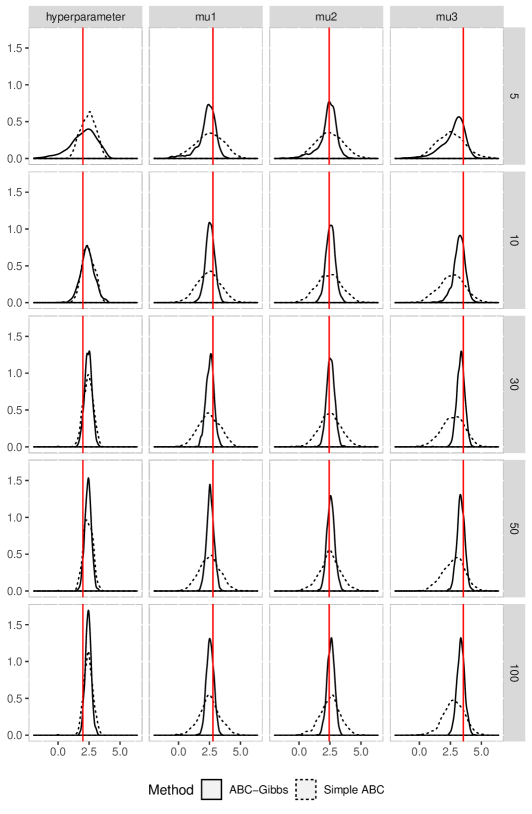
Figure 1: Comparison of the posterior density estimates of the hyperparameter and the first three parameter components of the hierarchical model of Equation 2 obtained with ABC and ABC-Gibbs, with identical computational cost. For ABC-Gibbs, results were computed with $N=1000$ Gibbs iterations; each row is labeled with the number $N_{\alpha}=N_{\mu}$ of iterations of the ABC scheme to update one parameter component. Red vertical lines represents the true values used to simulate the data.

To check the robustness of our method, we represent in Figure 2, 10 realisations of the posterior densities, for $N=\lfloor 1000/30\rfloor$, and $N_{\alpha}=N_{\mu}=30$ (with the first $5$ points in ABC-Gibbs removed to account for the small burn in). SMC-ABC does not allow for a fixed limit on the number of simulations, due to the resampling step. We used therefore $10^{4}$ particles, with a target of the smallest possible tolerance for a maximum of $30$ steps. In total, SMC-ABC was alloted roughly 60 times more simulations than ABC-Gibbs and ABC. The ABC-Gibbs density is overdispersed compared to the true posterior, albeit closer than the ABC, especially for the parameter $\mu_{1}$. On the other hand, SMC-ABC fails for this model: due to the difficulties resulting from its high dimension, an adaptive version fails to produce interesting proposals, notwithstanding a consistently larger computational budget. The distribution approximation on $\alpha$ is however better than its ABC counterpart. This fact is supported by numerical experiments in lower dimensions where all three methods lead to suitable approximations, as illustrated in the supplementary material, Section 8.2. The improvement brought by ABC-Gibbs in high dimension occurs consistently over simulations.

This experiment further highlights a striking differenciation between ABC-SMC methods, which require a significant degree of calibration when no package is readily available, and ABC-Gibbs, which relies on a straightforward implementation, reproduced in the supplementary material.

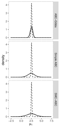
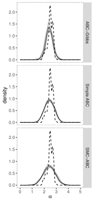
Figure 2: Posterior densities for 10 replicas of the algorithms compared to the exact posterior density. The true posterior is represented by the dashed line.

4 Application: hierarchical G & K distribution

The G & K distribution is a notorious example (Prangle, 2017) of an intractable distribution. It depends on parameters $(\mu,B,g,k)$ and is defined by its inverse cumulative distribution function

$$F^{-1}(x;\mu,B,g,k,c)=\mu+B\left(1+c\frac{1-e^{-gz(x)}}{1+e^{-gz(x)}}\right)\left(1+z(x)^{2}\right)^{k}z(x)$$

where $z$ is the quantile function of the standard normal distribution, and $c$ is a constant typically set to $0.8$ (Prangle, 2017). While the likelihood function is intractable, it is straightforward to simulate realisations of this distribution, making it a favourite benchmark for ABC methods (see for instance Fearnhead & Prangle, 2012).

Here, we analyse two hierarchical versions of this model, both of the form:

$$\mu_{i}\sim\mathcal{N}(\alpha,1)\qquad x_{i}\sim gk(\mu_{i},B,g,k)\qquad i=1,\ldots,n\,.$$ (3)

In a first experiment, we assume that the parameters $B$, $g$ and $k$ are known and we infer the position parameters $(\mu_{i})$. This leads to the graphical model represented on the left of Figure 3. We refer to this model as the simple hierarchical G & K model.

Figure 3: Left: Simple hierarchical G & K model; Right: doubly hierarchical G & K model

For a hyperprior $\alpha\sim\mathcal{U}[-10,10]$, the assumptions of Theorem 11.1 are satisfied. Figure 4 compares the results of our algorithm with those of ABC for a similar computational cost in dimension $n=50$, and ABC-SMC (same as before) for a higher computational cost, with $1000$ particles, $500$ iterations leading to a computational cost roughly $20$ times longer. As in Section 3.2, ABC-Gibbs outperforms both other methods: Vanilla ABC is overdispersed, and carefully calibrated ABC-SMC is either highly peaked at the wrong location or producing results similar with ABC.

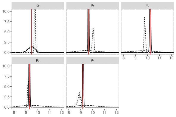
Figure 4: Posterior approximations for the simple hierarchical G & K model. The $y$ axis is truncated as the ABC-SMC pseudo-posterior is very peaked. The red vertical lines identify the value of the parameters used in the simulation.

As a second experiment, we infer all parameters ($B$, $g$, $k$, $\alpha$ and the $\mu_{i}$) in Equation 3, with independent hyperpriors $\alpha\sim\mathcal{U}(-10,10)$ and $B,g,k\sim\mathcal{U}(0,1)$. This corresponds to the graphical model represented on the right of Figure 3, which we refer to as a doubly hierarchical G & K model. The same summary statistic is used at every step of the algorithm, namely the octiles of the observations. Let $q(x,p)$ be the $p$-th quantile of sample $x$ and take two observations $x_{1}$ and $x_{2}$; our distance function is

$$d(x_{1},x_{2})=\sum_{i=0}^{8}\left|q\left(x_{1},i/8\right)-q\left(x_{2},i/8\right)\right|.$$

It is straightforward to that the assumptions of Theorem 2.2 are satisfied by this model, when considering the parameters in the order $\alpha,B,g,k,(\mu_{i})$.

Figures 4, 5 and 6 compare the output of ABC-Gibbs with Vanilla ABC and ABC-SMC in the same implementation as before, under a fixed budget of $2\cdot 10^{6}$ model simulations for ABC-Gibbs and ABC; ABC-SMC is run with $10^{3}$ particles, for $500$ steps, resulting in a a grand total computational cost larger than $2.5\cdot 10^{7}$ simulations. Note that there exist analytical approximations of the G & K posterior that give better results than ABC methods in the non hierarchical case, however none of these methods can be easily extended to the hierarchical case.

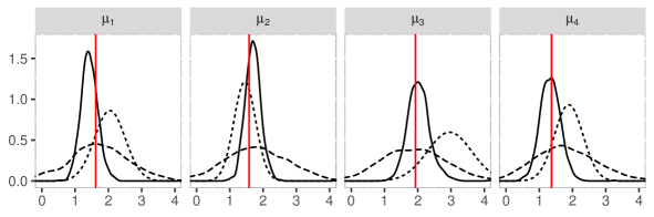
Figure 5: Posterior densities for the first four parameters, among 50, $\mu_{1},\dots,\mu_{4}$ in the doubly hierarchical $g$ & $k$ model.

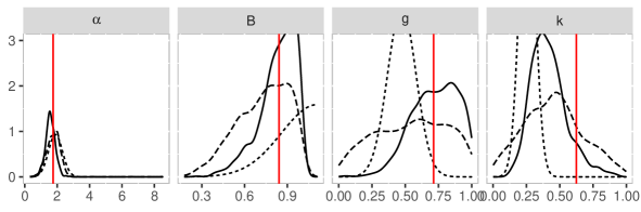
Figure 6: Posterior densities for the top-level parameters $\alpha$, $B$, $g$ and $k$ in the doubly hierarchical $g$ & $k$ model

The simple and double hierarchical G & K models lead to comparable results. ABC-Gibbs provides consistently better results (that are more concentrated around the true value), than ABC. The approximation provided by ABC-SMC is less peaked and occasionaly exhibits a bias, if less visible in the hyperaparameter case. Sequential Monte Carlo is supposed to iteratively reduce the threshold of the approximation; however, due to the difficulty of calibrating, the starting points, the reduction is quite slow. It is thus unlikely a further increase in the computational time would lead to higher improvements.

In Section 10 of the Supplementary material, we consider another example (a hierarchical Moving Average model), for which the results are similar.

5 Example with full dependence

The concept of ABC-Gibbs is by no means restricted to hierarchical settings. It applies in full generality to any decomposition or completion of the parameter ${\theta}$ into $n$ terms, $(\theta_{1},\ldots,\theta_{n})$. For simplicity’s sake, we only analyse below the case of $n=2$ parameters, and furthermore assume that $\theta_{1}$ and $\theta_{2}$ are a priori independent. The extension to $n\geq 2$ parameters, or non-independent parameters, is straightforward though cumbersome. The generic Algorithm 3 and Theorem 2.1 can thus be adapted to non-hierarchical models where ${\theta}=(\theta_{1},\theta_{2})$, such that the conditional posteriors $\pi(\theta_{1}\mid x^{\star},\theta_{2})$ and $\pi(\theta_{2}\mid x^{\star},\theta_{1})$ depend on the entire dataset $x^{\star}$ rather than a significantly smaller subset. This setting implies that the approximation steps in ABC-Gibbs will mostly require the simulation of objects of the same size as in ABC.

When the statistics $s_{1}$ and $s_{2}$ are identical, a single distance can be used, with $\varepsilon_{1}=\varepsilon_{2}$. The resulting stationary distribution is then the same as for ABC, since it is proportional to

$$\int\pi(\theta_{1})\pi(\theta_{2})f(x\mid\theta_{1},\theta_{2})\mathbf{1}_{\eta\{s_{1}(x),s_{1}(x^{\star})\}\leq\varepsilon_{1}}\,\mathrm{d}x.$$

Formally, these statistics should however be different, since more efficient and smaller-dimension statistics can be calibrated to each parameter.

As an illustration, consider an example inspired by inverse problems (Kaipio & Fox, 2011), in a simplified version. These problems, although deterministic, are difficult to tackle with traditional methods, as the likelihood function is typically extremely expensive to compute (Neal, 2012), requiring the use of surrogate models, and thus approximations. Let $y$ be the solution of the heat equation on a circle defined for $(\tau,z)\in]0,T]\times[0,1[$ by

$$\partial_{\tau}y(z,\tau)=\partial_{z}\left\{\theta(z)\partial_{z}y(z,\tau)\right\},$$

with $\theta(z)=\sum_{j=1}^{n}\theta_{j}\mathbf{1}_{\{(j-1)/n,j/n\}}(z)$ and with boundary conditions $y(z,0)=y_{0}(z)$ and $y(0,\tau)=y(1,\tau)$. We assume $y_{0}$ known and the parameter is $\theta=(\theta_{1},\dots,\theta_{n})$. The equation is discretized towards its numerical resolution. For this purpose, the first order finite elements method relies on discretisation steps of size $1/n$ for $z$ and $\Delta$ for $\tau$. A stepwise approximation of the solution is thus $\hat{y}(z,t)=\sum_{j=1}^{n}y_{j,t}\phi_{j}(z)$, where, for $j<n$, $\phi_{j}(z)=(1-|nz-j|)\mathbf{1}_{|nz-j|<1}$ and $\phi_{n}(z)=(1-nz)\mathbf{1}_{0<z<1/n}+(nz-n+1)\mathbf{1}_{1-1/n<z<1}$, and with $y_{j,t}$ defined by

$$\frac{y_{j,t+1}-y_{j,t}}{3\Delta}+\frac{y_{j+1,t+1}-y_{j+1,t}}{6\Delta} +\frac{y_{j-1,t+1}-y_{j-1,t}}{6\Delta}$$

$$\quad=y_{j,t+1}(\theta_{j+1}+\theta_{j})-y_{j-1,t+1}\theta_{j}-y_{j+1,t+1}\theta_{j+1}.$$

We then observe a noisy version of this process, chosen as $x_{j,t}=\mathcal{N}(\hat{y}_{j,t},\sigma^{2})$.

In ABC-Gibbs, each parameter $\theta_{m}$ is updated with summary statistics the observations at locations $m-2,m-1,m,m+1$. ABC relies on the whole data as statistic. In the experiments, $n=20$ and $\Delta=0.1$, with a prior $\theta_{j}\sim\mathcal{U}[0,1]$, independently. Theorem 2.2 applies to this setting.

We compared both methods, using as above the same simulation budget and several experiments with various values of $N_{\varepsilon}$, keeping the total number of simulations constant at $N_{\text{tot}}=N_{\varepsilon}\cdot N=8\cdot 10^{6}$. As $N_{\varepsilon}$ increases, the size $N$ of the posterior sample decreases. Figure 7 illustrates the estimations of $\theta_{1}$. The ABC-Gibbs estimate is much closer to the true value of the parameter $\theta_{1}=0.75$, with a smaller variance. We emphasize once more that the choice of the ABC table size is critical, as for a fixed computational budget we must reach a balance between, on the one hand, the quality of the approximations of the conditionals (improved by increasing $N_{\varepsilon}$), and on the other hand Monte-Carlo error and convergence of the algorithm, (improved by increasing $N$). In our case, $N_{\varepsilon}=10$ was clearly the best choice (low bias and low variance). While we have no systematic rule to choose this parameter, we however advise to choose it so that the approximation of the conditional is significantly different from the prior when run separately.

As in previous instances, ABC-Gibbs is much more efficient than ABC. For instance, Figure 8 shows that the posterior sample of $\theta_{1}$ is more peaked around the true value for ABC-Gibbs. We repeated this experiment for a wide range of values for $\theta$. In all, ABC-Gibbs gives estimates close to the true value, and is never outperformed by ABC. This is confirmed by evaluating the expectation of the posterior predictive distance to the whole data, ABC-Gibbs achieves an average of $39.2\pm 0.002$, and ABC reaches an average of $103.8\pm 0.002$, based on 100 replicates.

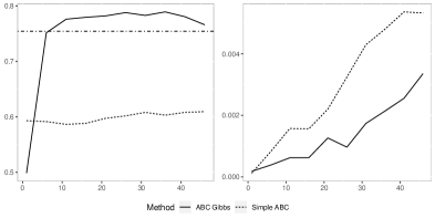
Figure 7: For the heat equation model, mean and variance of the ABC and ABC-Gibbs estimators of $\theta_{1}$ as $N_{\varepsilon}$ increases, selected from among 20 parameters. The horizontal line shows the true value of $\theta_{1}$.

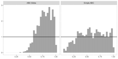
Figure 8: For the model of section 5, approximate posterior of $\theta_{1}$ compared with the uniform prior (black line) for ABC-Gibbs (right) and ABC (left)

6 Nature of the limiting distribution

When addressing hierarchical models of the form of Equation (1), we gave conditions in Theorem 2.2 for Algorithm 3 to have a limiting distribution $\nu_{\varepsilon}$. However, we did not specify the nature of this limiting distribution. We also showed that as the tolerance parameter $\varepsilon$ goes to 0, $\nu_{\varepsilon}$ tends to the stationary distribution $\nu_{0}$ of a Gibbs sampler with generators $\pi(\alpha)\pi(s_{\alpha}(\mu)\mid\alpha)$ and $\pi(\mu\mid\alpha)\pi(s_{\mu}(x)\mid\mu)$. It is possible that these generators are incompatible, that is, that there is no joint distribution associated with them. In such settings, the stationary distribution $\nu_{0}$ does not enjoy these generators as conditionals. The incompatibility of conditionals may seem contradictory with the fact that our algorithm does converge to a distribution, but in the case of a compact parameter space there always exists a limiting distribution, the main issue being rather that the limiting distribution has no straightforward Bayesian interpretation.

There are however specific situations where there are theoretical guarantees that the limiting distribution $\nu_{0}$ is in fact the posterior distribution associated with the summary statistics. According to Arnold & Press (1989) a necessary and sufficient condition for the conditionals to be compatible is the existence of two measurable functions $u(\alpha)$ and $v(\mu)$ such that

$$\frac{\pi(\alpha)\pi(s_{\alpha}(\mu)\mid\alpha)}{\pi(\mu\mid\alpha)f(s_{\mu}(x)\mid\mu)}=u(\alpha)v(\mu).$$

In particular, this occurs if $s_{\alpha}$ is sufficient. (This condition is not necessary, as it is also true for example if $s_{\alpha}$ is ancillary, although this is of limited interest.)

We have thus proven the following Proposition,

Proposition 6.1.

Under the assumptions of Theorems 2.1 and 2.3, a limiting distribution exists and converges, for both $\varepsilon_{\mu}$ and $\varepsilon_{\alpha}$ decreasing to $0$, to the stationary distribution of a Gibbs sampler with conditionals:

$$\pi(\alpha)\pi(s_{\alpha}(\mu)\mid\alpha)\text{ and }\pi(\mu\mid\alpha)f(s_{\mu}(x)\mid mu).$$

If $s_{\alpha}$ is sufficient, this limiting distribution is merely $\pi(\alpha,\mu)\pi(s_{\mu}(x)\mid\mu)$, that is the limiting distribution of ABC with summary statistic $s_{\mu}$ when the tolerance goes to $0$.

We can state similar results for non hierarchical models, although each model requires its own proof. For example, for the full dependency model 5 with two parameters $\theta_{1}$ and $\theta_{2}$ we have the following Proposition:

Proposition 6.2.

If $\pi(\theta_{1},\theta_{2})$ = $\pi(\theta_{1})\pi(\theta_{2})$ and $s_{\theta_{1}}=s_{\theta_{2}}$, as the tolerance $\varepsilon$ goes to zero and under the assumptions of Theorems 2.2 and 2.3, ABC-Gibbs and ABC have the same limiting distribution.

7 Discussion

The curse of dimensionality remains the major jamming block for the expansion of ABC methodology to more complex models as most of its avatars see their cost rise with the dimensions of the parameter and of the data (Li & Fearnhead, 2018b). This is particularly the case for high-dimensional parameters, since they require summary statistics that are at least of the same dimension and, unless the model under study is amenable to easily computed estimates of these parameters, a much larger collection of statistics is usually unavoidable. Breaking this curse of dimensionality by Gibbs-like steps is thus as important for ABC methods as it was for Monte Carlo methods (Gelfand & Smith, 1990), as relying on a small number of summary statistics facilitates the derivation of automated or semi-automated approaches (Fearnhead & Prangle, 2012; Raynal et al., 2019) and offers the potential for simulating pseudo-data of much smaller size. In appropriate settings, ABC-Gibbs sampling provides a noticeable improvement of the efficiency of approximate Bayesian computation methods. We have established some sufficient conditions for the convergence of ABC-Gibbs algorithms. Questions remain, from checking such conditions in practice to a better understanding of the limiting distributions from an inferential viewpoint. A Gibbs-like setting could also allow practitioners to embed their model in a higher-dimensional model with auxiliary variables, with compatible conditionals and improved computational tractability. In all cases, constructing or selecting a low-dimension informative summary statistic for the approximation of the conditionals might be an unavoidable challenge to further improve the quality of the results.

Component-wise Approximate Bayesian Computation via Gibbs-like steps: Supplementary Material

8 Supplementary material for Section 3.2

8.1 Checking the assumptions of Theorem 2.3

In this section, we show that the assumptions of Theorem 2.3 apply to the toy model of Equation 2 in Section 3.2.

We define $\mu_{-i}=(\mu_{1},\dots,\mu_{i-1},\mu_{i+1},\dots,\mu_{n})$. By conditional independence of the $\mu_{i}$ given $\alpha$, and choice of $s_{\mu}$, we have:

$$\pi_{\varepsilon_{\mu}}\{\cdot\mid s_{\mu}(x^{\star},\alpha,\mu_{-i})\}=\pi_{\varepsilon_{\mu}}\{\cdot\mid s_{\mu}(x^{\star}_{i},\alpha)\}$$

The assumptions to check can be rewritten as:

1. $\sup_{\alpha,\tilde{\alpha}}\|\pi_{\varepsilon_{\mu}}\{\cdot\mid s_{\mu}(x^{\star}_{1},\alpha)\}-\pi_{\varepsilon_{\mu}}\{\cdot\mid s_{\mu}(x^{\star}_{1},\tilde{\alpha})\}\|_{TV}<1/2$

3. $\sup_{\alpha,\tilde{\alpha}}\|\pi_{\varepsilon_{\mu}}\{\cdot\mid s_{\mu}(x^{\star}_{n},\alpha)\}-\pi_{\varepsilon_{\mu}}\{\cdot\mid s_{\mu}(x^{\star}_{n}),\tilde{\alpha}\}\|_{TV}<1/2$

4. $\sup_{\mu}\|\pi_{\varepsilon_{\alpha}}\{\cdot\mid s_{\alpha}(\mu)\}-\pi_{\varepsilon_{\alpha}}\{\cdot\mid s_{\alpha}(\mu)\}\|_{TV}<1/2$

To prove the assumption $(\mu_{i})$, we underline the fact that it is sufficient to check that there exists some subset $K$ of the parameter space, with positive measure for all hyperparameter $\alpha$, such that $\exists C>0,\forall\alpha,\forall\mu\in K$, $\pi_{\varepsilon_{\mu}}(\mu\mid\alpha,s(x^{*}))>C$.

We can compute these densities:

$$\pi_{\varepsilon}(\mu\mid\alpha,s(x^{*}))=\frac{\exp\{-(\mu-\alpha)^{2}/(2\tau)\int\exp(-(y-\mu)^{2}\sqrt{n}/(2\sigma)\}\mathbf{1}_{|y-\bar{x^{\star}}|<\varepsilon}\mathrm{d}y}{\int\exp\{-(\mu-\alpha)^{2}/(2\tau)\exp(-(y-\mu)^{2}\sqrt{n}/(2\sigma)\}\mathbf{1}_{|y-\bar{x^{\star}}|<\varepsilon}\mathrm{d}y\mathrm{d}\mu}.$$

As $\alpha$ is compactly supported on $[-4,4]$, the conditions are verified: we can roughly bound the probabilities by continuity of the expression.

The last condition $(\alpha)$ is always verified as we have by definition of the total variation distance:

$$\sup_{\mu}\|\pi_{\varepsilon_{\alpha}}(\cdot\mid\mu)-\pi_{\varepsilon_{\alpha}}(\cdot\mid\mu)\|_{TV}=0.$$

8.2 Comparison in dimension 3

In addition to the results shown in Figure 2, we show in Figure 9 a comparison of ABC-Gibbs, Vanilla ABC and SMC-ABC for the toy model of Section 3.2 in the low dimension case $n=2$.

As expected, in this low-dimension setting the results from SMC-ABC and Vanilla ABC are comparable to the approximate posterior provided by ABC-Gibbs for the parameter. ABC-Gibbs however seems to lead to a less stable approximation of the hyperparameter, this can be explained by the lower number of points (as we removed some of the first points as burn-in). This supports the idea that the behaviour of SMC-ABC in Figure 2 is caused by the high dimensionality. We believe that in higher dimension, SMC-ABC would require a very large number of particles, and a higher number of iteration each of which would cost much more in resampling, leading to a disastrous computational cost.

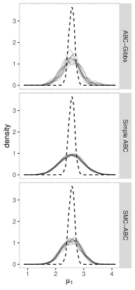
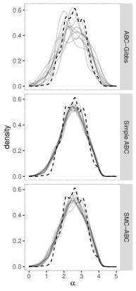
Figure 9: Parameter and hyperparameter for the Normal-Normal model with only two parameter and one hyperparameter.

8.3 Code example

⬇

gibbsparam <- function(data, hyper, var, sigm, nbeps, qq) {

#Gibbs step for the parameter, prior induced by the hyperparameter

p = length(data)

thetc = numeric(p)

dists=0

for (i in 1:p) {

thettest = rnorm(nbeps, hyper, var)

test = rowMeans(matrix(rnorm(qq * nbeps, thettest, sigm), nrow = nbeps))

dist = abs(test - data[i])

thetc[i] = thettest[which.min(dist)]

dists=dists+min(dist)

}

return(list(thetc,dists))

}

gibbshyper <- function(thet, nbeps2, var) {

#Gibbs step for the hyperparameter, with uniform prior

res = runif(nbeps2, -4, 4)

test = rowMeans(matrix(rnorm(length(thet) *

nbeps2, res, var), ncol=length(thet)))

dist = abs(test - mean(thet))

return(list(res[which.min(dist)],min(dist)))

}

gibbstot <- function(data, thetini, hyperini, sigm, var,

nbeps1, nbeps2, nbpts, qq) {

#full function

reshyper = rep(NA, nbpts + 1)

resparam = matrix(NA, ncol = nbpts + 1, nrow = length(thetini))

reshyper[1] = hyperini

resparam[,1] = thetini

resdist = rep(NA,nbpts)

for (i in 2:(nbpts + 1)) {

resdist[i-1]= 0

VV=gibbsparam(data, reshyper[i - 1], var, sigm, nbeps1, qq)

resparam[,i] = VV[[1]]

resdist[i-1]= resdist[i-1]+VV[[2]]

WW=gibbshyper(resparam[, i], nbeps2, var)

reshyper[i] = WW[[1]]

}

return(list(reshyper,resparam,resdist))

}

This exemplar code presents a simple implementation of ABC-Gibbs for the hierarchical normal model. The main function, gibbstot run iterations of Gibbs, it starts with an initial point thetini, hyperini and sample successively from the approximate conditionals for nbpts iterations.

Each of the approximate conditionals is sampled from by the functions gibbsparam and gibbshyper, as their name indicate the first one samples from $\pi_{\varepsilon_{\mu}}(\cdot\mid x,\alpha)$ and the second one $\pi_{\varepsilon_{\alpha}}(\cdot\mid x,\mu)$. Each one relies on the use of a fixed sized reference table of size nbeps1 et nbeps2. After having simulated points from the prior, pseudo data is simulated and compared (in the vectors test and dist) we return the point with smallest distance.

The other parameters var, sigm, qq correspond to the variance of the parameter given the hyperparameter, the variance of the observation given the parameters and the number of observation for each parameter, respectively.

9 Implementation of SMC-ABC

Our implementation of SMC-ABC merges the implementations of Del Moral et al. (2012) and Toni et al. (2008), in order to avoid degeneracy and arbitrary choice of the thresholds, as described in Algorithm 5.

Input: number of iterations $T$, $M\geq 1$, $\varepsilon_{0}$, $N\geq 0$, $N_{min}\leq N$, $\alpha>0$.

Output: a sample $(\theta_{1}^{0},\dots,\theta_{N}^{0})$ from an initial distribution $\pi^{0}$.

Compute for each of the value $\theta_{i}^{0}$ $M$ pseudo observations and the associated statistic stored in a vector $s^{i}_{0}$ of $M$ statistics;

Set $\varepsilon_{0}=\max_{i}(s_{i}^{0})$;

Set the weights $w_{i}^{0}=1/N$;

for $j=1,\ldots,T$ do

       Compute $\varepsilon_{j}$ and $w_{j}^{i}$ by solving $ESS(\{w^{i}_{j}\},\varepsilon_{j})=\alpha ESS(\{w^{i}_{j-1}\},\varepsilon_{j-1})$, where,

$$w_{j}^{i}\propto w_{j-1}^{i}\frac{\sum_{k=1}^{M}\mathbf{1}_{<\varepsilon_{j}}(s^{i}_{j-1}[k])}{\sum_{k=1}^{M}\mathbf{1}_{<\varepsilon_{j-1}}(s^{i}_{j-1}[k])}$$

if $ESS(\{w^{i}_{j}\},\varepsilon_{j})<N_{min}$ then

             Resample the value of the particles according to the weights $w_{j}^{i}$ ;

             We abusively use the same notation for the values after this step ;

             Set the new weights $w_{j}^{i}=1/N$

      for $i=1,\dots,N$ do

             do

                  Sample $\theta_{j}^{i*}\sim K_{j}(\theta_{j}^{i})$ and associated pseudo observations and statistics $s_{j}^{i*}$.

            while $\sum_{k=1}^{M}\mathbf{1}_{<\varepsilon_{j}}(s^{i*}_{j}[k])=0$;

            Set $\theta_{j}^{i}=\theta_{j}^{i*}$;

            

Algorithm 5 SMC-ABC

As underlined in Del Moral et al. (2012), we can choose the kernel $K_{j}$ so that it depends on the value of the particles. Following custom, we choose $K_{j}$ to be a Gaussian kernel with covariance matrix $2*Corr(\theta_{j}^{1},\dots,\theta_{j}^{N})$.

10 Supplementary material: Moving average example

10.1 Model and implementation

Figure 10: Hierarchical dependence structure used in the application of Section 10.3.

In this section, we study a hierarchical moving average model. A graphical representation of the hierarchy is shown in Figure 10. We denote $\mathcal{MA}_{2}(\mu,\sigma^{2})$ the distribution of a second order moving average model with parameters $\mu=(\mu_{1},\mu_{2})$ and $\sigma^{2}$, that is:

$$x(t)=y_{t}+\mu_{1}y_{t-1}+\mu_{2}y_{t-2}\,,\qquad\text{with }y_{t}\sim\mathcal{N}(0,\sigma^{2})\text{ for integer }t\geq-1.$$

We consider a hierarchical version of the $\mathcal{MA}_{2}$ model, consisting of $n$ parallel observed series and $3n+5$ parameters with the following dependencies and prior distributions: for $j=1,\ldots,n$,

$$x_{j}\sim\mathcal{MA}_{2}(\mu_{j},\sigma^{2}_{j})\,,\quad\sigma_{j}^{2}\sim\mathcal{IG}(\varsigma_{1},\varsigma_{2})\,,\quad\mu_{j}=\left(\beta_{j,1}-\beta_{j,2},2(\beta_{j,1}+\beta_{j,2})-1\right)=(\mu_{j,1},\mu_{j,2})\,,$$

where $(\beta_{j,1},\beta_{j,2},1-\beta_{j,1}-\beta_{j,2})\sim\mathcal{D}ir(\alpha_{1},\alpha_{2},\alpha_{3})$, and, if $\mathcal{E}$ denotes the exponential distribution and $\mathcal{C}_{+}$ the standard half-Cauchy distribution,

$$\alpha=(\alpha_{1},\alpha_{2},\alpha_{3})\sim\mathcal{E}(1)^{\otimes 3}\,,\quad\varsigma=(\varsigma_{1},\varsigma_{2})\sim\mathcal{C}_{+}^{\otimes 2}.$$

We denote $w(x_{j})$ the distance between the first two autocorrelations of $x_{j}$ and $x_{j}^{\star}$:

$$w^{2}(x_{j})=\{\rho_{1}(x_{j})-\rho_{1}(x^{\star}_{j})\}^{2}+\{\rho_{2}(x_{j})-\rho_{2}(x^{\star}_{j})\}^{2},$$

and

$$\overline{x_{j}}=\frac{1}{\lfloor T/3\rfloor}\sum_{t=1}^{\lfloor T/3\rfloor}x_{j}(3t)\,,\quad v(x_{j})=\frac{1}{\lfloor T/3\rfloor}\left|\sum_{t=1}^{\lfloor T/3\rfloor}(x_{j}(3t)-\overline{x_{j}})^{2}-\sum_{t=1}^{\lfloor T/3\rfloor}(x_{j}^{\star}(3t)-\overline{x_{j}^{\star}})^{2}\right|\,,$$

where $T$ is the length of the time series. The rationale is that for a $\mathcal{MA}_{2}$ model $x(t)$ and $x(t+3)$ are independent. Vanilla ABC uses a related single pseudo-distance defined by

$$\delta(x)=\sum_{j=1}^{n}\left\{\frac{w(x_{j})}{q_{j}}+\frac{v(x_{j})}{q_{j}^{\prime}}\right\}\,,$$ (4)

where $q_{j}$ and $q_{j}^{\prime}$ are the 0.1% quantiles of $w(x_{j})$ and $v(x_{j})$, respectively. This choice is constrained by the fact that these quantities appear to have undefined mean and variance.

For the current model, we have the following implementation: First, the $\mu_{j}$’s are updated using the pseudo-distance $d_{\mu_{j}}(x_{j},x_{j}^{*})=w(x_{j})$.

Second, the update of $\alpha$ relies on the sufficient statistic associated with Dirichlet distributions:

$$\bm{\mu}\mapsto\left(\sum_{j}\log\{(\mu_{j,2}+2\mu_{j,1}+1)/4\},\sum_{j}\log\{(\mu_{j,2}+2\mu_{j,1}+1)/4\}-\mu_{j,1})\right)$$

Third, the $\sigma_{j}$’s are updated using the pseudo-distance $d_{\sigma_{j}}(x_{j},x_{j}^{*})=v(x_{j})$. And last, $\varsigma$ is updated using the standard sufficient statistic associated with gamma distributions.

The two algorithms output samples from the two pseudo-posteriors. To compare the efficient of both samplers, we simulate new synthetic data from each parameter set in the output, and compute the distance (4) between observed and simulated samples, which is the distance used by ABC. If ABC-Gibbs produces a smaller value than the ABC sampler associated with this distance, this is an indicator of a better fit of the ABC-Gibbs distribution with the true posterior. As in the previous experiment, the total number of simulations of the time series is used as the default measure of the computational cost for the associated algorithm.

10.2 Toy dataset

Consider a synthetic dataset of $n=5$ times series each with length $T=100$. Both samplers return samples of size $N=1000$. The hyperparameters used to produce the true parameters and the simulated observed series are $\alpha=(1,2,3)$ and $\varsigma=(1,1)$. In ABC-Gibbs, the $\mu_{j}$’s are updated based on $N_{\mu}=1000$ time series, while the other parameters are updated based on $N_{\alpha}=N_{\sigma}=N_{\varsigma}=100$ replicas. The overall computational cost for ABC-Gibbs is $N_{\text{tot}}=5.5\cdot 10^{6}$, also used by ABC to run $1.1\cdot 10^{6}$ simulations of the whole hierarchy. The computational cost is slightly superior for ABC, as we have to simulate many more Dirichlet and Gamma random variables.

When evaluating the mean of the posterior predictive distance (4), ABC-Gibbs achieves an average of $274.1\pm 2.5$, and ABC an average of $436.8\pm 1.6$, based on 100 replicates. The sample output by ABC-Gibbs thus offers a noticeably better quality than the one generated by ABC from this perspective. The ABC output barely differs from a simulation from the prior, as shown in Figure 11 for the parameter $\mu_{1}$.

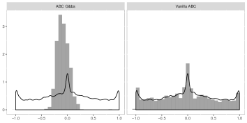
Figure 11: For the toy dataset of subsection 10.2, approximate posterior of $\mu_{1}$ compared with the prior for ABC-Gibbs (left) and ABC (right). The true value was $-0.06$.

10.3 Stellar flux

We now apply this model to stellar flux data. The 8GHz daily flux emitted by seven stellar objects is analysed in Lazio et al. (2008), and the data were made public by the Naval Research Laboratory: https://tinyurl.com/yxorvl4u. Once a few missing observations have been removed, Lazio et al. (2008) suggest that the model described in Section 10.1 may be well suited to these data, with $T=208$. In ABC-Gibbs, the $\mu_{j}$’s are updated based on $N_{\mu}=500$ time series, while the other parameters require $N_{\alpha}=N_{\varsigma}=N_{\sigma}=100$ replicas. (The overall computing time is the same for the toy and the current datasets, that is, one hour on an Intel Xeon CPU E5-2630 v4 with rate 2.20GHz.)

The average posterior distance to the observed sample is $232.8\pm 1.25$ for ABC-Gibbs and $535\pm 0.95$ for ABC. The poor fit of the latter is confirmed in Figure 12, as it again stays quite close to the prior for the $\mu$’s. Since our model differs from the one proposed in Lazio et al. (2008), estimators cannot be directly compared.

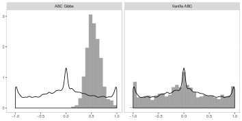
Figure 12: For the stellar dataset of subsection 10.3, approximate posterior of $\mu_{1}$ compared with the prior for ABC-Gibbs (left) and ABC (right)

11 Supplementary material: proofs of theorems

In this supplementary material, we define $\Theta_{j}$ as the domain of $\theta_{j}$. For the proofs that pertain to model (1) we define $\mathcal{A}$ as the domain of $\alpha$ and $\mathcal{B}$ as the domain of $\mu$. For a space $E$, $\mathcal{P}(E)$ is the space of the probability distributions over $E$.

11.1 Generalities on total variation distance

The main tool in our proofs is the total variation distance used by Nummelin (1978) and Meyn & Tweedie (1993). Let $\nu$ and $\tilde{\nu}$ be two probability distributions over the same space $E$. A coupling $\gamma$ between $\nu$ and $\tilde{\nu}$ is a probability distribution on $E\times E$ such that $\int\gamma(x,y)\mathrm{d}x=\nu$ and $\int\gamma(x,y)\mathrm{d}y=\tilde{\nu}$. Let $\Gamma(\nu,\tilde{\nu})$ denote the set of all couplings between $\nu$ and $\tilde{\nu}$. Then the total variation distance is defined as

$$\|\nu-\tilde{\nu}\|_{TV}=\frac{1}{2}\inf_{\gamma\in\Gamma(\nu,\tilde{\nu})}\mathrm{pr}(x\neq y\mid(x,y)\sim\gamma).$$

To handle this distance, we build an explicit coupling between the distributions: this provides an upper bound on the total variation distance. Note that there always exists an optimal coupling between two distributions, that is a coupling $\gamma_{0}$ such that $\|\nu-\tilde{\nu}\|_{TV}=\frac{1}{2}\mathrm{pr}(x\neq y\mid(x,y)\sim\gamma_{0})$.

11.2 Proof of Theorem 2.1

In this proof, we drop the conditionings on $x^{\star}$, $s_{1}$, and $s_{2}$, as they have no use in the computations and create a notational burden.

We only need to prove that the Markov chain $(\theta_{1}^{(i)})_{1\leq i\leq N}$ has a stationary distribution. We show that $Q\ :\mathcal{P}(\Theta_{1})\rightarrow\mathcal{P}(\Theta_{1})$, the mapping associated with the transition kernel, is a contraction; that is, we prove that there exists $L>1$ such that for all $\nu$ and $\tilde{\nu}$ in $\mathcal{P}(E)$

$$\|Q\nu-Q\tilde{\nu}\|_{TV}\leq L\|\nu-\tilde{\nu}\|_{TV}.$$

To build a coupling between $Q\nu$ and $Q\tilde{\nu}$ we construct a coupling kernel $\tilde{Q}:\mathcal{P}(\Theta_{1}\times\Theta_{1})\rightarrow\mathcal{P}(\Theta_{1}\times\Theta_{1})$, which takes a coupling $\xi_{0}$ as argument, such that $\int\tilde{Q}\xi_{0}(x,y)\mathrm{d}x=Q\nu(y)$ and $\int\tilde{Q}\xi_{0}(x,y)\mathrm{d}y=Q\tilde{\nu}(x)$. This coupling kernel is explicitly defined by the following procedure, which takes as input $(\theta_{1},\tilde{\theta}_{1})\sim\xi_{0}$ a coupling of $\nu$ and $\tilde{\nu}$, and returns $(\theta_{1}^{\prime},\tilde{\theta}_{1}^{\prime})\sim\tilde{Q}\xi_{0}$:

Input: $(\theta_{1},\tilde{\theta}_{1})\sim\xi_{0}$, $\xi_{1}(\cdot\mid\theta_{1},\tilde{\theta}_{1})$ an optimal coupling between $\pi_{\varepsilon_{2}}(\cdot\mid\theta_{1})$ and $\pi_{\varepsilon_{2}}(\cdot\mid\tilde{\theta}_{1})$, $\xi_{2}(\cdot\mid\theta_{2},\tilde{\theta}_{2})$ an optimal coupling between $\pi_{\varepsilon_{1}}(\cdot\mid\theta_{2})$ and $\pi_{\varepsilon_{1}}(\cdot\mid\tilde{\theta}_{2})$.

Output: $(\theta_{1}^{\prime},\tilde{\theta}_{1}^{\prime})\sim\tilde{Q}\xi_{0}$.

$(\theta_{2},\tilde{\theta}_{2})\sim\xi_{1}(\cdot\mid\theta_{1},\tilde{\theta}_{1})$;

$(\theta_{1}^{\prime},\tilde{\theta}_{1}^{\prime})\sim\xi_{2}(\cdot\mid\theta_{2},\tilde{\theta}_{2})$.

Algorithm 6 Coupling procedure for Theorem 2.1

This procedure satisfies the property that if $\theta_{1}=\tilde{\theta}_{1}$ then $\theta_{1}^{\prime}=\tilde{\theta}_{1}^{\prime}$, since for any distribution $\nu_{0}$, the optimal coupling between $\nu_{0}$ and itself is $(x,y)\mapsto\nu_{0}(x)\delta_{x=y}$.

The proofs choose $\xi_{0}$ as the optimal coupling between $\nu$ and $\tilde{\nu}$. In the following, $\tilde{\gamma}=\tilde{Q}\xi_{0}$, so that

$$\begin{split}\|Q\nu-Q\tilde{\nu}\|_{TV}&=\frac{1}{2}\inf_{\gamma\in\Gamma(Q\nu,Q\tilde{\nu})}\mathrm{pr}(\theta_{1}^{\prime}\neq\tilde{\theta}_{1}^{\prime}\mid(\theta_{1},\tilde{\theta}_{1})\sim\gamma)\\ &\leq\frac{1}{2}\mathrm{pr}(\theta_{1}^{\prime}\neq\tilde{\theta}_{1}^{\prime}\mid\theta_{1}=\tilde{\theta}_{1},(\theta_{1}^{\prime},\tilde{\theta}_{1}^{\prime})\sim\tilde{\gamma})\mathrm{pr}_{\xi_{0}}(\theta_{1}=\tilde{\theta}_{1})\\ &\hskip 28.45274pt+\frac{1}{2}\mathrm{pr}(\theta_{1}^{\prime}\neq\tilde{\theta}_{1}^{\prime}\mid\theta_{1}\neq\tilde{\theta}_{1},(\theta_{1}^{\prime},\tilde{\theta}_{1}^{\prime})\sim\tilde{\gamma})\mathrm{pr}_{\xi_{0}}(\theta_{1}\neq\tilde{\theta}_{1})\\ &\leq\frac{1}{2}\mathrm{pr}(\theta_{1}^{\prime}\neq\tilde{\theta}_{1}^{\prime}\mid\theta_{1}\neq\tilde{\theta}_{1},(\theta_{1}^{\prime},\tilde{\theta}_{1}^{\prime})\sim\tilde{\gamma})\mathrm{pr}_{\xi_{0}}(\theta_{1}\neq\tilde{\theta}_{1})\\ &\leq\|\nu-\tilde{\nu}\|_{TV}\mathrm{pr}(\theta_{1}^{\prime}\neq\tilde{\theta}_{1}^{\prime}\mid\theta_{1}\neq\tilde{\theta}_{1},(\theta_{1}^{\prime}\neq\tilde{\theta}_{1}^{\prime})\sim\tilde{\gamma}).\\ \end{split}$$

It is now sufficient to bound $\mathrm{pr}(\theta_{1}^{\prime}\neq\tilde{\theta}_{1}^{\prime}\mid\theta_{1}\neq\tilde{\theta}_{1},(\theta_{1}^{\prime},\tilde{\theta}_{1}^{\prime})\sim\tilde{\gamma})=1-\mathrm{pr}(\theta_{1}^{\prime}=\tilde{\theta}_{1}^{\prime}\mid\theta_{1}\neq\tilde{\theta}_{1},(\theta_{1}^{\prime},\tilde{\theta}_{1}^{\prime})\sim\tilde{\gamma})$, that is to find a lower bound on the probability that two different values $\theta_{1}$ and $\tilde{\theta}_{1}$ transition to the same value.

If $\theta_{2}=\tilde{\theta}_{2}$ then necessarily, $\theta_{1}^{\prime}=\tilde{\theta}_{1}^{\prime}$, in other words, if the coupling is successful at the first step of the procedure it is sufficient. This means that a lower bound on the coupling probability is the coupling probability at the first step of the procedure. Now,

$$\mathrm{pr}(\theta_{1}^{\prime}=\tilde{\theta}_{1}^{\prime}\mid\theta_{1}\neq\tilde{\theta}_{1},(\theta_{1}^{\prime},\tilde{\theta}_{1}^{\prime})\sim\tilde{\gamma})\geq 1-2\|\pi_{\varepsilon}(\cdot\mid\theta_{1})-\pi_{\varepsilon}(\cdot\mid\tilde{\theta}_{1})\|_{TV}$$

$$\geq 1-2\kappa>0.$$

This proves that the map $Q:\nu\mapsto Q\nu$ is a contraction. The space of all measures on $\mathcal{A}$ is complete when endowed with the total variation distance. Furthermore, the subspace of all probability distributions on $\Theta_{1}$ is stable by $Q$. Hence, by the Banach fixed-point theorem, it enjoys a fixed point and in particular the sequence $(Q^{n}\pi)$, with $\pi$ an arbitrary prior distribution, converges to this fixed point with rate $1-2\kappa$.

11.3 Proof of Theorem 2.3

The assumptions on $L_{2}$ and $L_{0}$ imply with the triangular inequality that the assumptions of Theorem 2.1 are verified, and thus that $\mu_{\varepsilon}$ exists.

In this proof, we need a coupling between two chains with different transition kernels. Let $\nu_{\varepsilon}$ be the target distribution of the approximate Gibbs sampler and $\nu_{0}$ be the target distribution of the exact Gibbs sampler. Let $(\theta_{1},\tilde{\theta}_{1})$ be a realisation of an optimal coupling $\xi_{0}$ between $\nu_{\varepsilon}$ and $\nu_{0}$. As before we propose a coupling procedure:

Input: $(\theta_{1},\tilde{\theta}_{1})\sim\xi_{0}$, $\xi_{3}(\cdot\mid\theta_{1},\tilde{\theta}_{1})$ an optimal coupling between $\pi_{\varepsilon}(\cdot\mid\theta_{1})$ and $\pi(\cdot\mid\tilde{\theta}_{1})$, $\xi_{4}(\cdot\mid\theta_{2},\tilde{\theta}_{2})$ an optimal coupling between $\pi_{\eta}(\cdot\mid\theta_{2})$ and $\pi(\cdot\mid\tilde{\theta}_{2})$.

Output: $(\theta_{1}^{\prime},\tilde{\theta}_{1}^{\prime})\sim\tilde{Q}\xi_{0}$.

$(\theta_{2},\tilde{\theta}_{2})\sim\xi_{3}(\cdot\mid\theta_{1},\tilde{\theta}_{1})$;

$(\theta_{1}^{\prime},\tilde{\theta}_{1}^{\prime})\sim\xi_{4}(\cdot\mid\theta_{2},\tilde{\theta}_{2})$.

Algorithm 7 Coupling procedure for Theorem 2.3

As the distributions $\nu_{\varepsilon}$ and $\nu_{0}$ are stationary for the evolution process, we have

$$\mathrm{pr}(\theta_{1}^{\prime}\neq\tilde{\theta}_{1}^{\prime})= \mathrm{pr}(\theta_{1}^{\prime}\neq\tilde{\theta}_{1}^{\prime}\mid\theta_{1}\neq\tilde{\theta}_{1})\mathrm{pr}(\theta_{1}\neq\tilde{\theta}_{1})+\mathrm{pr}(\theta_{1}^{\prime}\neq\tilde{\theta}_{1}^{\prime}\mid\theta_{1}=\tilde{\theta}_{1})\mathrm{pr}(\theta_{1}^{\prime}=\tilde{\theta}_{1}^{\prime})$$

$$\leq \frac{\mathrm{pr}(\theta_{1}^{\prime}\neq\tilde{\theta}_{1}^{\prime}\mid\theta_{1}=\tilde{\theta}_{1})}{\mathrm{pr}(\theta_{1}^{\prime}=\tilde{\theta}_{1}^{\prime}\mid\theta_{1}\neq\tilde{\theta}_{1})}.$$

As before we use a rough bound on the denominator:

$$\mathrm{pr}(\theta_{1}^{\prime}=\tilde{\theta}_{1}^{\prime}\mid\theta_{1}\neq\tilde{\theta}_{1})\geq (1-2\sup_{\varepsilon}\sup_{\theta_{1},\tilde{\theta}_{1}}\|\pi_{\varepsilon}(\cdot\mid\theta_{1})-\pi(\cdot\mid\tilde{\theta}_{1})\|_{TV})$$

$$\geq 1-2L_{0}.$$

For the numerator, we have, with $\theta_{2}$ and $\tilde{\theta}_{2}$ the transitory values of the second parameter,

$$\mathrm{pr}(\theta_{1}^{\prime}\neq\tilde{\theta}_{1}^{\prime}\mid\theta_{1}=\tilde{\theta}_{1}) \leq\mathrm{pr}(\theta_{1}^{\prime}\neq\tilde{\theta}_{1}^{\prime}\mid\theta_{2}=\tilde{\theta}_{2})\mathrm{pr}(\theta_{2}\neq\tilde{\theta}_{2}\mid\theta_{1}=\tilde{\theta}_{1})$$

$$\hskip 56.9055pt+\mathrm{pr}(\theta_{1}^{\prime}\neq\tilde{\theta}_{1}^{\prime}\mid\theta_{2}\neq\tilde{\theta}_{2})\mathrm{pr}(\theta_{2}\neq\tilde{\theta}_{2}\mid\theta_{1}=\tilde{\theta}_{1})$$

$$\leq\sup_{\theta_{2}}\mathrm{pr}\{\theta_{1}\neq\tilde{\theta}_{1}\mid(\theta_{1},\tilde{\theta}_{1})\sim\xi_{4}(\cdot\mid\theta_{2},\theta_{2})\}+\sup_{\vartheta_{1}}\mathrm{pr}\{\theta_{2}\neq\tilde{\theta}_{2}\mid(\theta_{2},\tilde{\theta}_{2})\sim\xi_{3}(\cdot\mid\vartheta_{1},\vartheta_{1})\}$$

$$\leq 2L_{1}(\varepsilon_{1})+2L_{2}(\varepsilon_{2})$$

Putting together both estimates gives the bound of the theorem.

11.4 Proofs specific to the hierarchical case

In addition to the general theorems presented in the main paper, we provide in this subsection convergence results which are specific to hierarchical models, with assumptions which may be more intuitive or easier to verify. specific convergence results. They are based on a particular implementation of ABC-Gibbs, presented for $n=1$ and in the case of an analytically available conditional density $\pi(\mu\mid\alpha,x^{\star})$, in Algorithm 8. We will gradually weaken the assumptions to finally prove Theorem 11.1:

Theorem 11.1.

Assume there exists a non-empty convex set $C$ with positive prior measure such that

$$\kappa_{1}= \inf_{s_{\alpha}(\mu)\in C}\pi(B_{s_{\alpha}(\mu),\varepsilon_{\alpha}/4})>0\,,$$

$$\kappa_{2}= \inf_{\alpha}\inf_{s_{\alpha}(\mu)\in C}\pi_{\varepsilon_{\mu}}\{B_{s_{\alpha}(\mu),3\varepsilon_{\alpha}/2}\mid s_{\mu}(x^{\star},\alpha),\alpha\}>0\,,$$

$$\kappa_{3}= \inf_{\alpha}\pi_{\varepsilon_{\mu}}\{s_{\alpha}(\mu)\in C\mid s_{\mu}(x^{\star},\alpha)\}>0\,,$$

where $B_{z,h}$ denotes the ball of centre $z$ and radius $h$. Then the Markov chain produced by Algorithm 4 converges geometrically in total variation distance to a stationary distribution $\nu_{\varepsilon}$, with geometric rate $1-\kappa_{1}\kappa_{2}\kappa_{3}^{2}$.

The rate in Theorem 11.1 is uninformative, as it is specific to the selected implementation.

Input: $\alpha^{(0)}\sim\pi(\alpha)$, $\mu^{(0)}\sim\pi(\mu\mid\alpha^{(0)})$.

Output: A sample $(\alpha^{(i)},\mu^{(i)})_{1\leq i\leq N}$.

for $i=1,\dots,N$ do

       $\mu^{c}\sim\pi(\cdot\mid\alpha^{(i-1)},x^{\star})$

      $\alpha^{c}\sim\pi$

      $\tilde{\mu}\sim\pi(\cdot\mid\alpha^{c})$

      if $\eta\{s_{\alpha}({\mu}),s_{\alpha}(\mu^{c})\}<\varepsilon_{\alpha}$ then

             $\mu^{(i+1)}\leftarrow\mu^{c}$

            $\alpha^{(i+1)}\leftarrow\alpha^{c}$

      else

             $\mu^{(i+1)}\leftarrow\mu^{(i)}$

            $\alpha^{(i+1)}\leftarrow\alpha^{(i)}$

Algorithm 8 Implementation of ABC-Gibbs used in the proofs.

First we state the most restrictive result:

Theorem 11.2.

Assume that the following conditions are both satisfied:

$$\kappa_{1} =\inf_{\mu}\pi(B_{s_{\alpha}(\mu),\varepsilon_{\alpha}/4})>0$$

$$\kappa_{2} =\inf_{\alpha}\inf_{\mu}\pi(B_{s_{\alpha}(\mu),3\varepsilon_{\alpha}/2}\mid\alpha,x)>0.$$

Then, the Markov chain associated with Algorithm 8 enjoys an invariant distribution, and it converges geometrically to this invariant measure with rate $1-\kappa_{1}\kappa_{2}$ for the total variation distance.

Proof 11.3.

The technique of the proof is essentially similar to that of Theorem 2.1. Let $\nu$ and $\tilde{\nu}$ be two distributions over $\mathcal{A}$. We describe the evolution of $\alpha,\tilde{\alpha}$ into $\alpha^{\prime},\tilde{\alpha}^{\prime}$, though the kernel $\tilde{Q}$. We denote $\mu,\tilde{\mu}$ the transitory second parameter.

Input: $(\alpha,\tilde{\alpha})$.

Output: $(\alpha^{\prime},\tilde{\alpha}^{\prime})$.

if $\alpha\neq\tilde{\alpha}$ then

      $(\mu,\tilde{\mu})\sim\pi(\cdot\mid\alpha,x)\otimes\pi(\cdot\mid\tilde{\alpha},x)$

else

      $\mu=\tilde{\mu}\sim\pi(\mu\mid\alpha,x)$

$\alpha^{c}\sim\pi$

$\mu^{c}\sim\pi(\cdot\mid\alpha^{c})$;

if $\eta\{s_{\alpha}(\mu),s_{\alpha}(\mu^{c})\}\leq\varepsilon_{\alpha}$ then

      $\alpha^{\prime}\leftarrow\alpha^{c}$

else

      $\alpha^{\prime}\leftarrow\alpha$

if $\eta\{s_{\alpha}(\tilde{\mu}),s_{\alpha}(\mu^{c})\}\leq\varepsilon_{\alpha}$ then

      $\tilde{\alpha}^{\prime}\leftarrow\alpha^{c}$

else

       $\tilde{\alpha}^{\prime}\leftarrow\tilde{\alpha}$

Algorithm 9 Coupling procedure

This process defines a transition kernel $\tilde{Q}$ for two coupled chains. As in the previous proofs, if $\alpha=\tilde{\alpha}$ then $\alpha^{\prime}=\tilde{\alpha}^{\prime}$.

Let $(\alpha,\tilde{\alpha})\sim\xi$, an optimal coupling between $\nu$ and $\tilde{\nu}$. Then,

$$\begin{split}\|Q\nu-Q\tilde{\nu}\|_{TV}&=\frac{1}{2}\inf_{\gamma\in\Gamma(Q\nu,Q\tilde{\nu})}\mathrm{pr}(\alpha^{\prime}\neq\tilde{\alpha}^{\prime}\mid(\alpha^{\prime},\tilde{\alpha}^{\prime})\sim\gamma)\\ &\leq\frac{1}{2}\mathrm{pr}_{\xi}(\alpha^{\prime}\neq\tilde{\alpha}^{\prime}\mid\alpha=\tilde{\alpha},(\alpha^{\prime},\tilde{\alpha}^{\prime})\sim\tilde{Q}\xi)\mathrm{pr}_{\xi}(\alpha=\tilde{\alpha})\\ &\hskip 28.45274pt+\frac{1}{2}\mathrm{pr}_{\xi}(\alpha^{\prime}\neq\tilde{\alpha}^{\prime}\mid\alpha\neq\tilde{\alpha},(\alpha^{\prime},\tilde{\alpha}^{\prime})\sim\tilde{Q}\xi)\mathrm{pr}_{\xi}(\alpha\neq\tilde{\alpha})\\ &\leq\frac{1}{2}\mathrm{pr}_{\xi}(\alpha^{\prime}\neq\tilde{\alpha}^{\prime}\mid\alpha\neq\tilde{\alpha},(\alpha^{\prime},\tilde{\alpha}^{\prime})\sim\tilde{Q}\xi)\mathrm{pr}_{\xi}(\alpha\neq\tilde{\alpha})\\ &\leq\|\nu-\tilde{\nu}\|_{TV}\mathrm{pr}_{\xi}(\alpha^{\prime}\neq\tilde{\alpha}^{\prime}\mid\alpha\neq\tilde{\alpha},(\alpha^{\prime},\tilde{\alpha}^{\prime})\sim\tilde{Q}\xi).\\ \end{split}$$

It is sufficient to find a uniform upper bound on $\mathrm{pr}_{\nu,\tilde{\nu}}(\alpha^{\prime}\neq\tilde{\alpha}^{\prime}\mid\alpha\neq\tilde{\alpha},(\alpha^{\prime},\tilde{\alpha}^{\prime})\sim\tilde{Q}\xi)=\int\pi\{s_{\alpha}(\mu^{c})\notin B_{s_{\alpha}(\mu),\varepsilon_{\alpha}}\cap B_{s_{\alpha}(\tilde{\mu}),\varepsilon_{\alpha}}\}\pi(\mu\mid\alpha,x)\pi(\tilde{\mu}\mid\tilde{\alpha},x)\nu(\alpha)\tilde{\nu}(\tilde{\alpha})\,\mathrm{d}\tilde{\alpha}\mathrm{d}\mu\mathrm{d}\tilde{\mu}$. Notice that we can choose our coupling $\xi$ such that conditionally on $\alpha\neq\tilde{\alpha}$ the marginals are independent.

$$\mathrm{pr}_{\nu,\tilde{\nu}}(\alpha^{\prime}\neq\tilde{\alpha}^{\prime}\mid\alpha\neq\tilde{\alpha})= \int\pi\left\{(B_{s_{\alpha}(\mu),\varepsilon_{\alpha}}\cap B_{s_{\alpha}(\tilde{\mu}),\varepsilon_{\alpha}})^{c}\right\}\pi(\mu\mid\alpha,x)$$

$$\hskip 28.45274pt\times\pi(\tilde{\mu}\mid\tilde{\alpha},x)\nu(\alpha)\tilde{\nu}(\tilde{\alpha})\,\mathrm{d}\alpha\mathrm{d}\tilde{\alpha}\mathrm{d}\mu\mathrm{d}\tilde{\mu}$$

$$= \int\pi\left\{(B_{s_{\alpha}(\mu),\varepsilon_{\alpha}}\cap B_{s_{\alpha}(\tilde{\mu}),\varepsilon_{\alpha}})^{c}\right\}\pi(\mu\mid\alpha,x)$$

$$\hskip 28.45274pt\times\pi(\tilde{\mu}\mid\tilde{\alpha},x)\nu(\alpha)\tilde{\nu}(\tilde{\alpha})\mathbf{1}_{\{\eta\{s_{\alpha}(\mu),s_{\alpha}(\tilde{\mu})\}\leq 3\varepsilon_{\alpha}/2\}}\,\mathrm{d}\alpha\mathrm{d}\tilde{\alpha}\mathrm{d}\mu\mathrm{d}\tilde{\mu}$$

$$+\int\pi\left\{(B_{s_{\alpha}(\mu),\varepsilon_{\alpha}}\cap B_{s_{\alpha}(\tilde{\mu}),\varepsilon_{\alpha}})^{c}\right\}\pi(\mu\mid\alpha,x)$$

$$\hskip 28.45274pt\times\pi(\tilde{\mu}\mid\tilde{\alpha},x)\nu(\alpha)\tilde{\nu}(\tilde{\alpha})\mathbf{1}_{\{\eta\{s_{\alpha}(\mu),s_{\alpha}(\tilde{\mu})\}>3\varepsilon_{\alpha}/2\}}\,\mathrm{d}\alpha\mathrm{d}\tilde{\alpha}\mathrm{d}\mu\mathrm{d}\tilde{\mu}$$

$$= I_{1}+I_{2}.$$

We now bound $I_{1}$ and $I_{2}$.

$$I_{1}= \int\pi\left\{(B_{s_{\alpha}(\mu),\varepsilon_{\alpha}}\cap B_{s_{\alpha}(\tilde{\mu}),\varepsilon_{\alpha}})^{c}\right\}\pi(\mu\mid\alpha,x)\pi(\tilde{\mu}\mid\tilde{\alpha},x)\nu(\alpha)\tilde{\nu}(\tilde{\alpha})\mathbf{1}_{\{\eta\{s_{\alpha}(\mu),s_{\alpha}(\tilde{\mu})\}\leq 3\varepsilon_{\alpha}/2\}}\mathrm{d}\tilde{\alpha}\mathrm{d}\alpha\mathrm{d}\mu\mathrm{d}\tilde{\mu}$$

$$\leq \int\pi(B_{\frac{s_{\alpha}(\mu)+s_{\alpha}(\tilde{\mu})}{2},\varepsilon_{\alpha}/4}^{c})\pi(\mu\mid\alpha,x)\pi(\tilde{\mu}\mid\tilde{\alpha},x)\nu(\alpha)\mathbf{1}_{\{\eta\{s_{\alpha}(\mu),s_{\alpha}(\tilde{\mu})\}\leq 3\varepsilon_{\alpha}/2\}}\nu(\tilde{\alpha})\mathrm{d}\alpha\mathrm{d}\tilde{\alpha}\mathrm{d}\mu\mathrm{d}\tilde{\mu}$$

$$\leq \mathrm{pr}_{\nu,\tilde{\nu}}\{\eta\{s_{\alpha}(\mu),s_{\alpha}(\tilde{\mu})\}\leq 3\varepsilon_{\alpha}/2\}$$

$$\hskip 28.45274pt-\int\pi(B_{\frac{s_{\alpha}(\mu)+s_{\alpha}(\tilde{\mu})}{2},\varepsilon_{\alpha}/2})\pi\{s_{\alpha}(\tilde{\mu})\in B_{s_{\alpha}(\mu),3\varepsilon_{\alpha}/2}\mid\tilde{\alpha},x\}\pi(\mu\mid\alpha,x)\nu(\alpha)\tilde{\nu}(\tilde{\alpha})\mathrm{d}\alpha\mathrm{d}\tilde{\alpha}\mathrm{d}\mu\mathrm{d}\tilde{\mu}$$

$$\leq \mathrm{pr}_{\nu,\tilde{\nu}}\{\eta\{s_{\alpha}(\mu),s_{\alpha}(\tilde{\mu})\}\leq 3\eta/2\}$$

$$\hskip 28.45274pt-\kappa_{1}\int\pi\{s_{\alpha}(\tilde{\mu})\in B_{s_{\alpha}(\mu),3\varepsilon_{\alpha}/2}\mid\tilde{\alpha},x\}\pi(\mu\mid\alpha,x)\nu(\alpha)\tilde{\nu}(\tilde{\alpha})\mathrm{d}\alpha\mathrm{d}\tilde{\alpha}\mathrm{d}\mu$$

$$\leq \mathrm{pr}_{\nu,\tilde{\nu}}\{\eta\{s_{\alpha}(\mu),s_{\alpha}(\tilde{\mu})\}\leq 3\varepsilon_{\alpha}/2\}-\kappa_{1}\kappa_{2}$$

$$I_{2}= \int\pi\left\{(B_{s_{\alpha}(\mu),\varepsilon_{\alpha}}\cap B_{s_{\alpha}(\tilde{\mu}),\varepsilon_{\alpha}})^{c}\right\}\pi(\mu\mid\alpha,x)\pi(\tilde{\mu}\mid\tilde{\alpha},x)\nu(\alpha)\tilde{\nu}(\tilde{\alpha})\mathbf{1}_{\{\eta\{s_{\alpha}(\mu),s_{\alpha}(\tilde{\mu})\}>3\varepsilon_{\alpha}/2\}}\mathrm{d}\alpha\mathrm{d}\tilde{\alpha}\mathrm{d}\mu\mathrm{d}\tilde{\mu}$$

$$\leq \pi(\mu\mid\alpha,x)\pi(\tilde{\mu}\mid\tilde{\alpha},x)\nu(\alpha)\mathbf{1}_{\eta\{s_{\alpha}(\mu),s_{\alpha}(\tilde{\mu})\}>3\varepsilon_{\eta}/2}\tilde{\nu}(\tilde{\alpha})\mathrm{d}\alpha\mathrm{d}\tilde{\alpha}\mathrm{d}\mu\mathrm{d}\tilde{\mu}$$

$$\leq \mathrm{pr}_{\nu,\tilde{\nu}}\{\eta\{s_{\alpha}(\mu),s_{\alpha}(\tilde{\mu})\}>3\varepsilon_{\eta}/2\}$$

Finally, putting both inequalities together, we have $I_{1}+I_{2}\leq 1-\kappa_{1}\kappa_{2}$, with $\kappa_{1}\kappa_{2}>0$ and

$$\|Q\nu-Q\tilde{\nu}\|_{TV} \leq(1-\kappa_{1}\kappa_{2})\|\nu-\tilde{\nu}\|_{TV}.$$

The conclusion is the same as in the proof of Theorem 2.1.

Remark 11.4.

In the proof, when we describe the coupling kernel, we generate $\mu$ and $\tilde{\mu}$ independently if $\alpha$ and $\tilde{\alpha}$ are different and as a single $\mu$ if they are equal. This is a particular coupling of the distributions $\pi(\cdot\mid\alpha,x)$ and $\pi(\cdot\mid\tilde{\alpha},x)$. Here, the link between Theorem 2.1 and this one becomes clear, as we make the coupling explicit toward reaching a bound in total variation.

We now relax the assumptions. First, we remove the assumption that $\mathcal{A}$ is compact: the resulting theorem is Theorem 11.1.

Proof 11.5.

With the same notations as before, we merely need to find a lower bound :

$$I_{3}=\int\mathrm{pr}(\mu^{c}\in B_{\frac{s_{\alpha}(\mu)+s_{\alpha}(\tilde{\mu})}{2},\varepsilon_{\alpha}/2})\pi(\mu\mid\alpha,x)\pi(\tilde{\mu}\mid\tilde{\alpha},x)\mu(\alpha)\nu(\tilde{\alpha})\mathbf{1}_{\{\eta\{s_{\alpha}(\mu),s_{\alpha}(\tilde{\mu})\}>3\varepsilon_{\alpha}/2\}}\mathrm{d}\alpha\mathrm{d}\tilde{\alpha}\mathrm{d}\mu\mathrm{d}\tilde{\mu}$$

$$I_{3}\geq \int\mathrm{pr}(B_{\frac{s_{\alpha}(\mu)+s_{\alpha}(\tilde{\mu})}{2},\varepsilon_{\alpha}/2})\pi(\mu\mid\alpha,x)\pi(\tilde{\mu}\mid\tilde{\alpha},x)\nu(\alpha)\tilde{\nu}(\tilde{\alpha})$$

$$\hskip 28.45274pt\times\mathbf{1}_{\{s_{\alpha}(\mu)+s_{\alpha}(\tilde{\mu})\}/2\in C\}}\mathbf{1}_{\{\eta\{s_{\alpha}(\mu),s_{\alpha}(\tilde{\mu})\}>3\varepsilon_{\alpha}/2\}}\mathrm{d}\alpha\mathrm{d}\tilde{\alpha}\mathrm{d}\mu\mathrm{d}\tilde{\mu}$$

$$+\int\mathrm{pr}(\mu\in B_{\frac{s_{\alpha}(\mu)+s_{\alpha}(\tilde{\mu})}{2},\varepsilon_{\alpha}/2})\pi(\mu\mid\alpha,x)\pi(\tilde{\mu}\mid\tilde{\alpha},x)\nu(\alpha)\tilde{\nu}(\tilde{\alpha})$$

$$\hskip 28.45274pt\times\mathbf{1}_{\{s_{\alpha}(\mu)+s_{\alpha}(\tilde{\mu})\}/2\notin C\}}\mathbf{1}_{\{\eta\{s_{\alpha}(\mu),s_{\alpha}(\tilde{\mu})\}>3\varepsilon_{\alpha}/2\}}\mathrm{d}\alpha\mathrm{d}\tilde{\alpha}\mathrm{d}\mu\mathrm{d}\tilde{\mu}$$

$$\geq \int\mathrm{pr}(\mu\in B_{\frac{s_{\alpha}(\mu)+s_{\alpha}(\tilde{\mu})}{2},\varepsilon_{\alpha}/2})\pi(\mu\mid\alpha,x)\pi(\tilde{\mu}\mid\tilde{\alpha},x)\nu(\alpha)\tilde{\nu}(\tilde{\alpha})$$

$$\hskip 28.45274pt\times\mathbf{1}_{\{s_{\alpha}(\mu)\in C\}}\mathbf{1}_{\{s_{\alpha}(\tilde{\mu})\in C\}}\mathbf{1}_{\{\eta\{s_{\alpha}(\mu),s_{\alpha}(\tilde{\mu})\{>3\varepsilon_{\alpha}/2\}}\mathrm{d}\alpha\mathrm{d}\tilde{\alpha}\mathrm{d}\mu\mathrm{d}\tilde{\mu}$$

$$\geq \kappa_{1}\kappa_{2}\kappa_{3}^{2}$$

as the convexity of $C$ ensures that $\mathbf{1}_{\{\{s_{\alpha}(\mu)+s_{\alpha}(\tilde{\mu})\}/2\in C\}}\geq\mathbf{1}_{s_{\alpha}(\mu)\in C}\mathbf{1}_{s_{\alpha}(\tilde{\mu})\in C}$.

We can remove the assumption that $\mathcal{B}$ is compact, by imposing a different assumption:

Theorem 11.6.

Assume that there exist $\mathcal{H}\subset\mathcal{P}(\mathcal{A})$ stable by $Q$ and $A\subset\mathcal{A}$ and $C\subset s_{\alpha}(\mathcal{B})$ with finite positive measure such that:

$$\kappa_{1} =\inf_{s_{\alpha}(\mu)\in C}\pi(B_{s_{\alpha}(\mu),\varepsilon_{\alpha}/4})>0;$$

$$\kappa_{2} =\inf_{\alpha\in A}\inf_{s_{\alpha}(\mu)\in C}\pi(B_{s_{\alpha}(\mu),3\varepsilon_{\alpha}/2}\mid\alpha,x)>0;$$

$$\kappa_{3} =\inf_{\alpha\in A}\pi\{s_{\alpha}(\mu)\in C\mid\alpha,x\}>0;$$

$$\kappa_{4} =\inf_{\nu\in\mathcal{H}}\nu(A)>0.$$

Then, the Markov chain associated with Algorithm 8 enjoys an invariant distribution and it converges geometrically to this invariant measure with rate $1-\kappa_{1}\kappa_{2}\kappa_{3}^{2}\kappa_{4}^{2}$.

Proof 11.7.

Similarly to previous proofs, we have

$$I_{3} \geq\int\mathrm{pr}(\mu\in B_{\frac{s_{\alpha}(\mu)+s_{\alpha}(\tilde{\mu})}{2},\varepsilon_{\alpha}/2})\pi(\mu\mid\alpha,x)\pi(\tilde{\mu}\mid\tilde{\alpha},x)\nu(\alpha)\tilde{\nu}(\tilde{\alpha})$$

$$\hskip 28.45274pt\times\mathbf{1}_{s_{\alpha}(\mu)\in C}\mathbf{1}_{s_{\alpha}(\tilde{\mu})\in C}\mathbf{1}_{\{\eta\{s_{\alpha}(\mu),s_{\alpha}(\tilde{\mu})\}>3\varepsilon_{\alpha}/2\}}\mathrm{d}\alpha\mathrm{d}\tilde{\alpha}\mathrm{d}\mu\mathrm{d}\tilde{\mu}$$

$$\geq\int\kappa_{1}\kappa_{2}\kappa_{3}^{2}\nu(\alpha)\tilde{\nu}(\tilde{\alpha})\mathbf{1}_{\alpha\in A}\mathbf{1}_{\tilde{\alpha}\in A}$$

$$\geq\kappa_{1}\kappa_{2}\kappa_{3}^{2}\kappa_{4}^{2}\,.$$

12 Supplementary material: Counter-example to Theorem 2.1

In this section, we give a simple example where the assumptions of Theorem 2.1 are not verified and where ABC-Gibbs fails (whereas Vanilla ABC does not).

Take a single observation from a mixture of two uniforms, with parameterized by $(\theta_{1},\theta_{2})$:

$$x\sim\frac{1}{2}\mathcal{U}(\theta_{1},\theta_{1}+1)+\frac{1}{2}\mathcal{U}(\theta_{2},\theta_{2}+1).$$

For the numerical applications, we shall use the realization $x^{\star}=5$. Consider the prior distribution

$$(\theta_{1},\theta_{2})\sim\mathcal{U}(\mathcal{A})\qquad\mathcal{A}=\left\{(\theta_{1},\theta_{2}):0\leq\theta_{1},\theta_{2}\leq 10\text{ and }|\theta_{1}-\theta_{2}|>2\right\}$$

The exact posterior is uniform over the set

$$\left\{\left([0,10]\times[x-1,x]\right)\cup\left([x-1,x]\times[0,10]\right)\right\}\cap\mathcal{A}.$$

The prior and exact posterior are shown in Figure 13, as well as the outcome of Vanilla ABC and ABC-Gibbs with $\varepsilon=\varepsilon_{1}=\varepsilon_{2}=0.5$. Vanilla ABC leads to a reasonable approximation of the posterior, but ABC-Gibbs misses half of the posterior. Other realizations of ABC-Gibbs lead to the symmetric pseudo-posterior, with the roles of $\theta_{1}$ and $\theta_{2}$ swapped. This is a situation where the ABC-Gibbs does not converge to a unique stationary distribution $\nu_{\varepsilon}$ (as soon as $\varepsilon_{1},\varepsilon_{2}\leq\frac{1}{2}$).

For Theorem 2.1 to apply, we would need

$$\sup_{\theta_{1},\tilde{\theta}_{1}}\|\pi_{\varepsilon_{2}}\{\cdot\mid s_{2}(x^{\star},\theta_{1})\}-\pi_{\varepsilon_{2}}\{\cdot\mid s_{2}(x^{\star},\tilde{\theta}_{1})\}\|_{TV}=\kappa<\frac{1}{2}.$$

Consider $\theta_{1}=1$ and $\tilde{\theta}_{1}=5$. Then $\pi_{\varepsilon_{2}}\{\cdot\mid s_{2}(x^{\star},\theta_{1})\}$ has support $[3.5,5.5]$ and $\pi_{\varepsilon_{2}}\{\cdot\mid s_{2}(x^{\star},\tilde{\theta}_{1})\}$ has support $[0,3]\cup[7,10]$. Since the two supports are disjoint, the distance in total variation between the two distributions is 1, and Theorem 2.1 does not apply. Intuitively, the Markov chain does not converge because it is not irreducible.

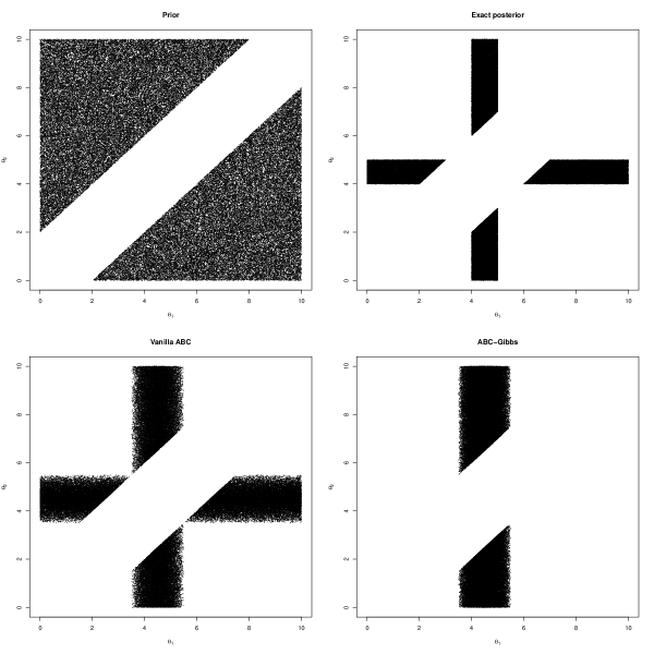
Figure 13: Illustration of the mixture of uniforms counter-example from Section 12, with $x^{\star}=5$ and $\varepsilon=0.5$. Top left: prior distribution. Top right: Exact posterior. Bottom left: Vanilla ABC posterior. Bottom right: one possible outcome of ABC-Gibbs. The Vanilla ABC is a reasonable approximation of the exact posterior, but the ABC-Gibbs outcome only covers half of the support.

References

- Arnold & Press (1989) Arnold, B. C. & Press, S. J. (1989). Compatible conditional distributions. Journal of the American Statistical Association 84, 152–156.
- Beaumont et al. (2009) Beaumont, M. A., Cornuet, J.-M., Marin, J.-M. & Robert, C. P. (2009). Adaptive approximate Bayesian computation. Biometrika 96, 983–990.
- Beaumont et al. (2002) Beaumont, M. A., Zhang, W. & Balding, D. J. (2002). Approximate Bayesian Computation in Population Genetics. Genetics 162, 2025–2035.
- Carlin & Louis (1996) Carlin, B. & Louis, T. (1996). Bayes and Empirical Bayes Methods for Data Analysis. London: Chapman and Hall.
- Csilléry et al. (2010) Csilléry, K., Blum, M. G. B., Gaggiotti, O. E. & François, O. (2010). Approximate Bayesian computation (ABC) in practice. Trends in Ecology & Evolution 25, 410–418.
- Del Moral et al. (2012) Del Moral, P., Doucet, A. & Jasra, A. (2012). An adaptive sequential Monte Carlo method for approximate Bayesian computation. Statistics and Computing 22, 1009–1020.
- Fearnhead & Prangle (2012) Fearnhead, P. & Prangle, D. (2012). Constructing summary statistics for approximate Bayesian computation: semi-automatic approximate Bayesian computation. Journal of the Royal Statistical Society. Series B 74, 419–474.
- Frazier et al. (2018) Frazier, D., Martin, G., Robert, C. & Rousseau, J. (2018). Asymptotic properties of approximate Bayesian computation. Biometrika 105, 593–607.
- Gelfand & Smith (1990) Gelfand, A. E. & Smith, A. F. M. (1990). Sampling-Based Approaches to Calculating Marginal Densities. Journal of the American Statistical Association 85, 398–409.
- Gelman et al. (2013) Gelman, A., Carlin, J. B., Stern, H. S., Dunson, D. B., Vehtari, A. & Rubin, D. B. (2013). Bayesian Data Analysis, Third Edition. Chapman & Hall/CRC Texts in Statistical Science. Taylor & Francis.
- Geman & Geman (1984) Geman, S. & Geman, D. (1984). Stochastic relaxation, Gibbs distributions and the Bayesian restoration of images. IEEE Trans. Pattern Anal. Mach. Intell. 6, 721–741.
- Kaipio & Fox (2011) Kaipio, J. P. & Fox, C. (2011). The Bayesian Framework for Inverse Problems in Heat Transfer. Heat Transfer Engineering 32, 718–753.
- Kousathanas et al. (2016) Kousathanas, A., Leuenberger, C., Helfer, J., Quinodoz, M., Foll, M. & Wegmann, D. (2016). Likelihood-free inference in high-dimensional models. Genetics 203, 893–904.
- Li & Fearnhead (2018a) Li, W. & Fearnhead, P. (2018a). Convergence of regression-adjusted approximate Bayesian computation. Biometrika 105, 301–318.
- Li & Fearnhead (2018b) Li, W. & Fearnhead, P. (2018b). On the asymptotic efficiency of approximate Bayesian computation estimators. Biometrika 105, 285–299.
- Lindley & Smith (1972) Lindley, D. & Smith, A. (1972). Bayes estimates for the linear model. Journal of the Royal Statistical Society. Series B 34, 1–41.
- Lunn et al. (2010) Lunn, D., Thomas, A., Best, N. & Spiegelhalter, D. (2010). The BUGS Book: A Practical Introduction to Bayesian Analysis. New York: Chapman & Hall/CRC Press.
- Marin et al. (2012) Marin, J.-M., Pudlo, P., Robert, C. P. & Ryder, R. J. (2012). Approximate Bayesian computational methods. Statistics and Computing 22, 1167–1180.
- Marjoram et al. (2003) Marjoram, P., Molitor, J., Plagnol, V. & Tavaré, S. (2003). Markov chain Monte Carlo without likelihoods. Proceedings of the National Academy of Sciences 100, 15324–15328.
- Moores et al. (2015) Moores, M. T., Drovandi, C. C., Mengersen, K. & Robert, C. P. (2015). Pre-processing for approximate Bayesian computation in image analysis. Statistics and Computing 25, 23–33.
- Neal (2012) Neal, P. (2012). Efficient likelihood-free Bayesian Computation for household epidemics. Statistics and Computing 22, 1239–1256.
- Nott et al. (2014) Nott, D. J., Fan, Y., Marshall, L. & Sisson, S. (2014). Approximate Bayesian computation and Bayes’ linear analysis: toward high-dimensional ABC. Journal of Computational and Graphical Statistics 23, 65–86.
- Prangle (2017) Prangle, D. (2017). gk: An R package for the -and- and generalised -and- distributions. arXiv preprint arXiv:1706.06889 .
- Raynal et al. (2019) Raynal, L., Marin, J.-M., Pudlo, P., Ribatet, M., Robert, C. P. & Estoup, A. (2019). ABC random forests for Bayesian parameter inference. Bioinformatics 35, 1720–1728.
- Robert & Casella (2004) Robert, C. & Casella, G. (2004). Monte Carlo Statistical Methods. New York: Springer Verlag, 2nd ed.
- Rodrigues et al. (2020) Rodrigues, G., Nott, D. J. & Sisson, S. (2020). Likelihood-free approximate Gibbs sampling. Statistics and Computing 30, 1057–1073.
- Sisson et al. (2018) Sisson, S., Fan, Y. & Beaumont, M., eds. (2018). Handbook of Approximate Bayesian Computation. New York: Chapman and Hall/CRC.
- Tavaré et al. (1997) Tavaré, S., Balding, D. J., Griffiths, R. C. & Donnelly, P. (1997). Inferring Coalescence Times From DNA Sequence Data. Genetics 145, 505–518.
- Toni et al. (2008) Toni, T., Welch, D., Strelkowa, N., Ipsen, A. & Stumpf, M. P. H. (2008). Approximate Bayesian computation scheme for parameter inference and model selection in dynamical systems. Journal of the Royal Society Interface 6, 187–202.
- Turner & Van Zandt (2013) Turner, B. & Van Zandt, T. (2013). Hierarchical approximate Bayesian computation. Psychometrika 79.
- Wilkinson et al. (2011) Wilkinson, R., Steiper, M., Soligo, C., Martin, R., Yang, Z. & Tavaré, S. (2011). Dating primate divergences through an integrated analysis of palaeontological and molecular data. Systematic Biology 60, 16–31.

References

- Del Moral et al. (2012) Del Moral, P., Doucet, A. & Jasra, A. (2012). An adaptive sequential Monte Carlo method for approximate Bayesian computation. Statistics and Computing 22, 1009–1020.
- Lazio et al. (2008) Lazio, T. J. W., B. Waltman, E., D. Ghigo, F., Fiedler, R., S. Foster, R. & K. J. Johnston, a. (2008). A Dual-Frequency, Multiyear Monitoring Program of Compact Radio Sources. The Astrophysical Journal Supplement Series 136, 265.
- Meyn & Tweedie (1993) Meyn, S. P. & Tweedie, R. L. (1993). Markov Chains and Stochastic Stability. London: Springer-Verlag.
- Nummelin (1978) Nummelin, E. (1978). A splitting technique for Harris recurrent chains. Zeit. Warsch. Verv. Gebiete 43, 309–318.
- Toni et al. (2008) Toni, T., Welch, D., Strelkowa, N., Ipsen, A. & Stumpf, M. P. H. (2008). Approximate Bayesian computation scheme for parameter inference and model selection in dynamical systems. Journal of the Royal Society Interface 6, 187–202.