ADMM for Efficient Deep Learning with Global Convergence

Abstract.

Alternating Direction Method of Multipliers (ADMM) has been used successfully in many conventional machine learning applications and is considered to be a useful alternative to Stochastic Gradient Descent (SGD) as a deep learning optimizer. However, as an emerging domain, several challenges remain, including 1) The lack of global convergence guarantees, 2) Slow convergence towards solutions, and 3) Cubic time complexity with regard to feature dimensions. In this paper, we propose a novel optimization framework for deep learning via ADMM (dlADMM) to address these challenges simultaneously. The parameters in each layer are updated backward and then forward so that the parameter information in each layer is exchanged efficiently. The time complexity is reduced from cubic to quadratic in (latent) feature dimensions via a dedicated algorithm design for subproblems that enhances them utilizing iterative quadratic approximations and backtracking. Finally, we provide the first proof of global convergence for an ADMM-based method (dlADMM) in a deep neural network problem under mild conditions. Experiments on benchmark datasets demonstrated that our proposed dlADMM algorithm outperforms most of the comparison methods.

1. Introduction

Deep learning has been a hot topic in the machine learning community for the last decade. While conventional machine learning techniques have limited capacity to process natural data in their raw form, deep learning methods are composed of non-linear modules that can learn multiple levels of representation automatically (lecun2015deep, ). Since deep learning methods are usually applied in large-scale datasets, such approaches require efficient optimizers to obtain a feasible solution within realistic time limits.
Stochastic Gradient Descent (SGD) and many of its variants are popular state-of-the-art methods for training deep learning models due to their efficiency. However, SGD suffers from many limitations that prevent its more widespread use: for example, the error signal diminishes as the gradient is backpropagated (i.e. the gradient vanishes); and SGD is sensitive to poor conditioning, which means a small input can change the gradient dramatically. Recently, the use of the Alternating Direction Method of Multipliers (ADMM) has been proposed as an alternative to SGD. ADMM splits a problem into many subproblems and coordinates them globally to obtain the solution. It has been demonstrated successfully for many machine learning applications (boyd2011distributed, ). The advantages of ADMM are numerous: it exhibits linear scaling as data is processed in parallel across cores; it does not require gradient steps and hence avoids gradient vanishing problems; it is also immune to poor conditioning (taylor2016training, ).
Even though the performance of the ADMM seems promising, there are still several challenges at must be overcome: 1. The lack of global convergence guarantees. Despite the fact that many empirical experiments have shown that ADMM converges in deep learning applications, the underlying theory governing this convergence behavior remains mysterious. This is because a typical deep learning problem consists of a combination of linear and nonlinear mappings, causing optimization problems to be highly nonconvex. This means that traditional proof techniques cannot be directly applied. 2. Slow convergence towards solutions. Although ADMM is a powerful optimization framework that can be applied to large-scale deep learning applications, it usually converges slowly to high accuracy, even for simple examples (boyd2011distributed, ). It is often the case that ADMM becomes trapped in a modest solution and hence performs worse than SGD, as the experiment described later in this paper in Section 5 demonstrates. 3. Cubic time complexity with regard to feature dimensions. The implementation of the ADMM is very time-consuming for real-world datasets. Experiments conducted by Taylor et al. found that ADMM required more than 7000 cores to train a neural network with just 300 neurons (taylor2016training, ). This computational bottleneck mainly originates from the matrix inversion required to update the weight parameters. Computing an inverse matrix needs further subiterations, and its time complexity is approximately $O(n^{3})$, where $n$ is a feature dimension (boyd2011distributed, ).
In order to deal with these difficulties simultaneously, in this paper we propose a novel optimization framework for a deep learning Alternating Direction Method of Multipliers (dlADMM) algorithm. Specifically, our new dlADMM algorithm updates parameters first in a backward direction and then forwards. This update approach propagates parameter information across the whole network and accelerates the convergence process. It also avoids the operation of matrix inversion using the quadratic approximation and backtracking techniques, reducing the time complexity from $O(n^{3})$ to $O(n^{2})$. Finally, to the best of our knowledge, we provide the first proof of the global convergence of the ADMM-based method (dlADMM) in a deep neural network problem. The assumption conditions are mild enough for many common loss functions (e.g. cross-entropy loss and square loss) and activation functions (e.g. rectified linear unit (ReLU) and leaky ReLU) to satisfy. Our proposed framework and convergence proof are highly flexible for fully-connected deep neural networks, as well as being easily extendable to other popular network architectures such as Convolutional Neural Networks (krizhevsky2012imagenet, ) and Recurrent Neural Networks (mikolov2010recurrent, ). Our contributions in this paper include:

• We present a novel and efficient dlADMM algorithm to handle the fully-connected deep neural network problem. The new dlADMM updates parameters in a backward-forward fashion to speed up the convergence process.

• We propose the use of quadratic approximation and backtracking techniques to avoid the need for matrix inversion as well as reducing the computational cost for large scale datasets. The time complexity of subproblems in dlADMM is reduced from $O(n^{3})$ to $O(n^{2})$.

• We investigate several attractive convergence properties of dlADMM. The convergence assumptions are very mild to ensure that most deep learning applications satisfy our assumptions. dlADMM is guaranteed to converge to a critical point globally (i.e., whatever the initialization is) when the hyperparameter is sufficiently large. We also analyze the new algorithm’s sublinear convergence rate.

• We conduct experiments on several benchmark datasets to validate our proposed dlADMM algorithm. The results show that the proposed dlADMM algorithm performs better than most existing state-of-the-art algorithms, including SGD and its variants.

The rest of this paper is organized as follows. In Section 2, we summarize recent research related to this topic. In Section 3, we present the new dlADMM algorithm, quadratic approximation, and the backtracking techniques utilized. In Section 4, we introduce the main convergence results for the dlADMM algorithm. The results of extensive experiments conducted to show the convergence, efficiency, and effectiveness of our proposed new dlADMM algorithm are presented in in Section 5, and Section 6 concludes this paper by summarizing the research.

2. Related Work

Previous literature related to this research includes optimization for deep learning models and ADMM for nonconvex problems.
Optimization for deep learning models: The SGD algorithm and its variants play a dominant role in the research conducted by deep learning optimization community. The famous back-propagation algorithm was firstly introduced by Rumelhart et al. to train the neural network effectively (rumelhart1986learning, ). Since the superior performance exhibited by AlexNet (krizhevsky2012imagenet, ) in 2012, deep learning has attracted a great deal of researchers’ attention and many new optimizers based on SGD have been proposed to accelerate the convergence process, including the use of Polyak momentum (polyak1964some, ), as well as research on the Nesterov momentum and initialization by Sutskever et al. (sutskever2013importance, ). Adam is the most popular method because it is computationally efficient and requires little tuning (kingma2014adam, ). Other well-known methods that incorporate adaptive learning rates include AdaGrad (duchi2011adaptive, ), RMSProp (tielemandivide, ), and AMSGrad (j.2018on, ). Recently, the Alternating Direction Method of Multipliers (ADMM) has become popular with researchers due to its excellent scalability (taylor2016training, ). However, even though these optimizers perform well in real-world applications, their convergence mechanisms remain mysterious. This is because convergence assumptions are not applicable to deep learning problems, which often require non-differentiable activation functions such as the Rectifier linear unit (ReLU).
ADMM for nonconvex problems: The good performance achieved by ADMM over a range wide of convex problems has attracted the attention of many researchers, who have now begun to investigate the behavior of ADMM on nonconvex problems and made significant advances. For example, Wang et al. proposed an ADMM to solve multi-convex problems with a convergence guarantee (wang2019multi, ), while Wang et al. presented convergence conditions for a coupled objective function that is nonconvex and nonsmooth (wang2015global, ). Chen et al. discussed the use of ADMM to solve problems with quadratic coupling terms (chen2015extended, ) and Wang et al. studied the convergence behavior of the ADMM for problems with nonlinear equality constraints (wang2017nonconvex, ). Even though ADMM has been proposed to solve deep learning applications (taylor2016training, ; gao2019incomplete, ), there remains a lack theoretical convergence analysis for the application of ADMM to such problems.

Table 1. Important Notations and Descriptions

Notations	Descriptions
$L$	Number of layers.
$W_{l}$	The weight matrix for the $l$-th layer.
$b_{l}$	The intercept vector for the $l$-th layer.
$z_{l}$	The temporary variable of the linear mapping for the $l$-th layer.
$f_{l}(z_{l})$	The nonlinear activation function for the $l$-th layer.
$a_{l}$	The output for the $l$-th layer.
$x$	The input matrix of the neural network.
$y$	The predefined label vector.
$R(z_{L},y)$	The risk function for the $l$-th layer.
$\Omega_{l}(W_{l})$	The regularization term for the $l$-th layer.
$n_{l}$	The number of neurons for the $l$-th layer.

3. The dlADMM Algorithm

We present our proposed dlADMM algorithm in this section. Section 3.1 formulates the deep neural network problem, Section 3.2 introduces how the dlADMM algorithm works, and the quadratic approximation and backtracking techniques used to solve the subproblems are presented in Section 3.3.

3.1. Problem Formulation

Table 1 lists the important notation utilized in this paper. Even though there are many variants of formulations for deep neural networks, a typical neural network is defined by multiple linear mappings and nonlinear activation functions. A linear mapping for the $l$-th layer is composed of a weight matrix $W_{l}\in\mathbb{R}^{n_{l}\times n_{l-1}}$ and an intercept vector $b_{l}\in\mathbb{R}^{n_{l}}$, where $n_{l}$ is the number of neurons for the $l$-th layer; a nonlinear mapping for the $l$-th layer is defined by a continuous activation function $f_{l}(\bullet)$. Given an input $a_{l-1}\in\mathbb{R}^{n_{l-1}}$ from the $(l-1)$-th layer, the $l$-th layer outputs $a_{l}=f_{l}(W_{l}a_{l-1}+b_{l})$. Obviously, $a_{l-1}$ is nested in $a_{l}=f_{l}(\bullet)$. By introducing an auxiliary variable $z_{l}$, the task of training a deep neural network problem is formulated mathematically as follows:

Problem 1.

$$\min\nolimits_{W_{l},b_{l},z_{l},a_{l}}R(z_{L};y)+\sum\nolimits_{l=1}^{L}\Omega_{l}(W_{l})$$

$$s.t.z_{l}=W_{l}a_{l-1}+b_{l}(l=1,\cdots,L),\ a_{l}=f_{l}(z_{l})\ \!(l=1,\cdots,L-1)$$

In Problem 1, $a_{0}=x\in\mathbb{R}^{n_{0}}$ is the input of the deep neural network where $n_{0}$ is the number of feature dimensions, and $y$ is a predefined label vector. $R(z_{L};y)$ is a risk function for the $L$-th layer, which is convex, continuous and proper, and $\Omega_{l}(W_{l})$ is a regularization term for the $l$-th layer, which is also convex, continuous, and proper. Rather than solving Problem 1 directly, we can relax Problem 1 by adding an $\ell_{2}$ penalty to address Problem 2 as follows:

Problem 2.

$$\min\nolimits_{W_{l},b_{l},z_{l},a_{l}}F(\textbf{W},\textbf{b},\textbf{z},\textbf{a})=R(z_{L};y)\!+\!\sum\nolimits_{l=1}^{L}\Omega_{l}(W_{l})$$

$$+(\nu/2)\sum\nolimits_{l=1}^{L-1}(\|z_{l}-W_{l}a_{l-1}-b_{l}\|^{2}_{2}+\|a_{l}-f_{l}(z_{l})\|^{2}_{2})$$

$$s.t.\ z_{L}=W_{L}a_{L-1}+b_{L}$$

where $\textbf{W}=\{W_{l}\}_{l=1}^{L}$, $\textbf{b}=\{b_{l}\}_{l=1}^{L}$, $\textbf{z}=\{z_{l}\}_{l=1}^{L}$, $\textbf{a}=\{a_{l}\}_{l=1}^{L-1}$ and $\nu>0$ is a tuning parameter. Compared with Problem 1, Problem 2 has only a linear constraint $z_{L}=W_{L}a_{L-1}+b_{L}$ and hence is easier to solve. It is straightforward to show that as $\nu\rightarrow\infty$, the solution of Problem 2 approaches that of Problem 1.

3.2. The dlADMM algorithm

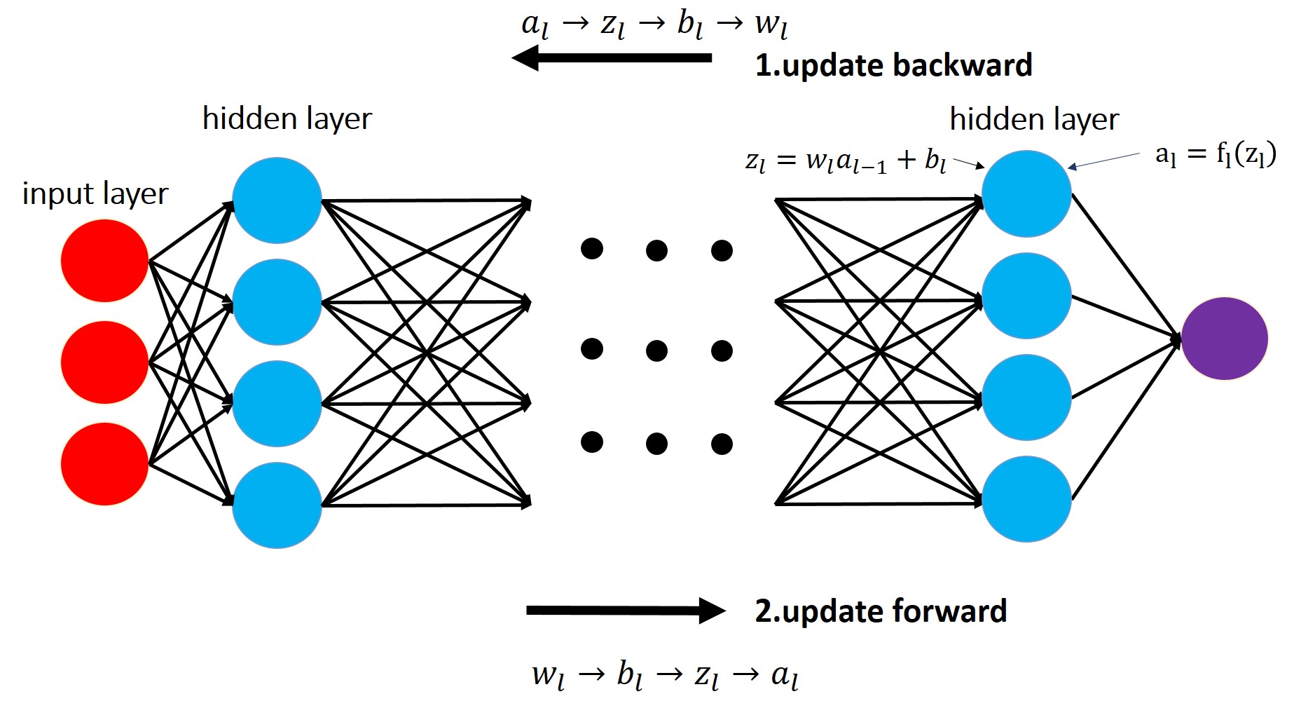
We introduce the dlADMM algorithm to solve Problem 2 in this section. The traditional ADMM strategy for optimizing parameters is to start from the first layer and then update parameters in the following layer sequentially (taylor2016training, ). In this case, the parameters in the final layer are subject to the parameter update in the first layer. However, the parameters in the final layer contain important information that can be transmitted towards the previous layers to speed up convergence. To achieve this, we propose our novel dlADMM framework, as shown in Figure 1. Specifically, the dlADMM algorithm updates parameters in two steps. In the first, the dlADMM begins updating from the $L$-th (final) layer and moves backward toward the first layer. The update order of parameters in the same layer is $a_{l}\rightarrow z_{l}\rightarrow b_{l}\rightarrow W_{l}$. In the second, the dlADMM reverses the update direction, beginning at the first layer and moving forward toward the $L$-th (final) layer. The update order of the parameters in the same layer is $W_{l}\rightarrow b_{l}\rightarrow z_{l}\rightarrow a_{l}$. The parameter information for all layers can be exchanged completely by adopting this update approach.

Figure 1. The dlADMM framework overview: update parameter backward and then forward.

Now we can present our dlADMM algorithm mathematically. The augmented Lagrangian function of Problem 2 is shown in the following form:

(1) $$L_{\rho}(\textbf{W}\!,\!\textbf{b},\!\textbf{z},\!\textbf{a},\!u)\!=R(z_{L};y)\!+\!\sum\nolimits_{l=1}^{L}\Omega_{l}(W_{l})\!+\phi(\textbf{W}\!,\!\textbf{b},\!\textbf{z},\!\textbf{a},u)$$

where $\phi(\textbf{W}\!,\!\textbf{b},\!\textbf{z},\!\textbf{a},\!u)=\!(\nu/2)\sum\nolimits_{l=1}^{L\!-\!1}(\|z_{l}\!-\!W_{l}\!a_{l\!-\!1}\!-\!b_{l}\|^{2}_{2}+\|a_{l}-f_{l}(z_{l})\|^{2}_{2})+u^{T}(z_{L}-W_{L}a_{L-1}-b_{L})+(\rho/2)\|z_{L}-W_{L}a_{L-1}-b_{L}\|^{2}_{2}$, $u$ is a dual variable and $\rho>0$ is a hyperparameter of the dlADMM algorithm. We denote $\overline{W}^{k+1}_{l}$, $\overline{b}^{k+1}_{l}$, $\overline{z}^{k+1}_{l}$ and $\overline{a}^{k+1}_{l}$ as the backward update of the dlADMM for the $l$-th layer in the $(k+1)$-th iteration , while ${W}^{k+1}_{l}$, ${b}^{k+1}_{l}$, ${z}^{k+1}_{l}$ and ${a}^{k+1}_{l}$ are denoted as the forward update of the dlADMM for the $l$-th layer in the $(k+1)$-th iteration. Moreover, we denote $\overline{\textbf{W}}^{k+1}_{l}=\{\{{W}^{k}_{i}\}_{i=1}^{l-1},\{\overline{{W}}^{k+1}_{i}\}_{i=l}^{L}\}$, $\overline{\textbf{b}}^{k+1}_{l}=\{\{{b}^{k}_{i}\}_{i=1}^{l-1},\{\overline{{b}}^{k+1}_{i}\}_{i=l}^{L}\}$, $\overline{\textbf{z}}^{k+1}_{l}=\{\{{z}^{k}_{i}\}_{i=1}^{l-1},\{\overline{{z}}^{k+1}_{i}\}_{i=l}^{L}\}$,
$\overline{\textbf{a}}^{k+1}_{l}=\{\{{a}^{k}_{i}\}_{i=1}^{l-1},\{\overline{{a}}^{k+1}_{i}\}_{i=l}^{L-1}\}$, ${\textbf{W}}^{k+1}_{l}=\{\{{W}^{k+1}_{i}\}_{i=1}^{l},\{\overline{{W}}^{k+1}_{i}\}_{i=l+1}^{L}\}$, ${\textbf{b}}^{k+1}_{l}=\{\{{b}^{k+1}_{i}\}_{i=1}^{l},\{\overline{{b}}^{k+1}_{i}\}_{i=l+1}^{L}\}$, ${\textbf{z}}^{k+1}_{l}=\{\{{z}^{k+1}_{i}\}_{i=1}^{l},\{\overline{{z}}^{k+1}_{i}\}_{i=l+1}^{L}\}$, ${\textbf{a}}^{k+1}_{l}=\{\{{a}^{k+1}_{i}\}_{i=1}^{l},\{\overline{{a}}^{k+1}_{i}\}_{i=l+1}^{L-1}\}$, $\overline{\textbf{W}}^{k+1}=\{\overline{W}_{i}^{k+1}\}_{i=1}^{L}$, $\overline{\textbf{b}}^{k+1}=\{\overline{b}_{i}^{k+1}\}_{i=1}^{L}$, $\overline{\textbf{z}}^{k+1}=\{\overline{z}_{i}^{k+1}\}_{i=1}^{L}$, $\overline{\textbf{a}}^{k+1}=\{\overline{a}_{i}^{k+1}\}_{i=1}^{L-1}$, $\textbf{W}^{k+1}=\{W_{i}^{k+1}\}_{i=1}^{L}$, $\textbf{b}^{k+1}=\{b_{i}^{k+1}\}_{i=1}^{L}$, $\textbf{z}^{k+1}=\{z_{i}^{k+1}\}_{i=1}^{L}$, and $\textbf{a}^{k+1}=\{a_{i}^{k+1}\}_{i=1}^{L-1}$. Then the dlADMM algorithm is shown in Algorithm 1. Specifically, Lines 5, 6, 10, 11, 14, 15, 17 and 18 solve eight subproblems, namely, $\overline{a}^{k+1}_{l}$, $\overline{z}^{k+1}_{l}$, $\overline{b}^{k+1}_{l}$, $\overline{W}^{k+1}_{l}$, ${W}^{k+1}_{l}$, ${b}^{k+1}_{l}$, ${z}^{k+1}_{l}$ and ${a}^{k+1}_{l}$, respectively. Lines 21 and 22 update the residual $r^{k+1}$ and the dual variable $u^{k+1}$, respectively.

Algorithm 1 the dlADMM Algorithm to Solve Problem 2

0: $y$, $a_{0}=x$, $\rho$, $\nu$.

0: $a_{l}(l=1,\cdots,L-1),W_{l}(l=1,\cdots,L),b_{l}(l=1,\cdots,L),z_{l}(l=1,\cdots,L)$.

1: Initialize $k=0$.

2: while $\textbf{W}^{k+1},\textbf{b}^{k+1},\textbf{z}^{k+1},\textbf{a}^{k+1}$ not converged do

3:    for $l=L$ to $1$ do

4:      if $l<L$ then

5:        Update $\overline{a}^{k+1}_{l}$ in Equation (3).

6:        Update $\overline{z}^{k+1}_{l}$ in Equation (4).

7:        Update $\overline{b}^{k+1}_{l}$ in Equation (6).

8:      else

9:        Update $\overline{z}^{k+1}_{L}$ in Equation (5).

10:        Update $\overline{b}^{k+1}_{L}$ in Equation (7).

11:      end if

12:      Update $\overline{W}^{k+1}_{l}$ in Equation (9).

13:    end for

14:    for $l=1$ to $L$ do

15:      Update ${W}^{k+1}_{l}$ in Equation (11).

16:      if $l<L$ then

17:        Update $b^{k+1}_{l}$ in Equation (12).

18:        Update $z^{k+1}_{l}$ in Equation (14).

19:        Update $a^{k+1}_{l}$ in Equation (16).

20:      else

21:        Update $b^{k+1}_{l}$ in Equation (13).

22:         Update $z^{k+1}_{L}$ in Equation (15).

23:        $r^{k+1}\leftarrow z_{L}^{k+1}-W^{k+1}_{L}a^{k+1}_{L-1}-b^{k+1}_{L}$.

24:        $u^{k+1}\leftarrow u^{k}+\rho r^{k+1}$.

25:      end if

26:    end for

27:    $k\leftarrow k+1$.

28: end while

29: Output $\textbf{W},\textbf{b},\textbf{z},\textbf{a}$.

3.3. The Quadratic Approximation and Backtracking

The eight subproblems in Algorithm 1 are discussed in detail in this section. Most can be solved by quadratic approximation and the backtracking techniques described above, so the operation of the matrix inversion can be avoided.

1. Update $\overline{a}^{k+1}_{l}$
The variables $\overline{a}^{k+1}_{l}(l=1,\cdots,L-1)$ are updated as follows:

$$\overline{a}^{k\!+\!1}_{l} \leftarrow\!\arg\min\nolimits_{a_{l}}\!L_{\rho}(\overline{\textbf{W}}^{k\!+\!1}_{l\!+\!1},\overline{\textbf{b}}^{k\!+\!1}_{l\!+\!1},\overline{\textbf{z}}^{k\!+\!1}_{l\!+\!1},\{a^{k}_{i}\}_{i\!=\!1}^{l\!-\!1},a_{l},\{\overline{a}^{k\!+\!1}_{i}\}_{i\!=\!l\!+\!1}^{L\!-\!1},u^{k})$$

The subproblem is transformed into the following form after it is replaced by Equation (1).

(2) $$\overline{a}^{k\!+\!1}_{l}\leftarrow\!\arg\!\min\nolimits_{a_{l}}\!\phi\!(\overline{\textbf{W}}^{k\!+\!1}_{l\!+\!1},\overline{\textbf{b}}^{k\!+\!1}_{l\!+\!1},\overline{\textbf{z}}^{k\!+\!1}_{l\!+\!1},\{a^{k}_{i}\}_{i\!=\!1}^{l\!-\!1}\!,a_{l},\{\overline{a}^{k\!+\!1}_{i}\}_{i\!=\!l\!+\!1}^{L\!-\!1}\!,\!u^{k})$$

Because $a_{l}$ and $W_{l+1}$ are coupled in $\phi(\bullet)$, in order to solve this problem, we must compute the inverse matrix of $\overline{W}^{k+1}_{l+1}$, which involves subiterations and is computationally expensive (taylor2016training, ). In order to handle this challenge, we define $\overline{Q}_{l}(a_{l};\overline{\tau}^{k+1}_{l})$ as a quadratic approximation of $\phi$ at $a^{k}_{l}$, which is mathematically reformulated as follows:

$$\overline{Q}_{l}(a_{l};\overline{\tau}^{k+1}_{l}) =\phi(\overline{\textbf{W}}^{k+1}_{l+1},\overline{\textbf{b}}^{k+1}_{l+1},\overline{\textbf{z}}^{k+1}_{l+1},\overline{\textbf{a}}^{k+1}_{l+1},u^{k})$$

$$+(\nabla_{a^{k}_{l}}\phi)^{T}(\overline{\textbf{W}}^{k+1}_{l+1},\overline{\textbf{b}}^{k+1}_{l+1},\overline{\textbf{z}}^{k+1}_{l+1},\overline{\textbf{a}}^{k+1}_{l+1},u^{k})(a_{l}-a^{k}_{l})$$

$$+\|\overline{\tau}^{k+1}_{l}\circ(a_{l}-a^{k}_{l})^{\circ 2}\|_{1}/2$$

where $\overline{\tau}^{k+1}_{l}>0$ is a parameter vector, $\circ$ denotes the Hadamard product (the elementwise product), and $a^{\circ b}$ denotes $a$ to the Hadamard power of $b$ and $\|\bullet\|_{1}$ is the $\ell_{1}$ norm. $\nabla_{a^{k}_{l}}\phi$ is the gradient of $\overline{a}_{l}$ at $a^{k}_{l}$. Obviously, $\overline{Q}_{l}(a^{k}_{l};\overline{\tau}^{k+1}_{l})=\phi(\overline{\textbf{W}}^{k+1}_{l+1},\overline{\textbf{b}}^{k+1}_{l+1},\overline{\textbf{z}}^{k+1}_{l+1},\overline{\textbf{a}}^{k+1}_{l+1},u^{k})$. Rather than minimizing the original problem in Equation (2), we instead solve the following problem:

(3) $$\overline{a}^{k+1}_{l} \leftarrow\arg\min\nolimits_{a_{l}}\overline{Q}_{l}(a_{l};\overline{\tau}^{k+1}_{l})$$

Because $\overline{Q}_{l}(a_{l};\overline{\tau}^{k+1}_{l})$ is a quadratic function with respect to $a_{l}$, the solution can be obtained by

$$\overline{a}^{k+1}_{l}\leftarrow a^{k}_{l}-\nabla_{a^{k}_{l}}\phi/\overline{\tau}^{k+1}_{l}$$

given a suitable $\overline{\tau}^{k+1}_{l}$. Now the main focus is how to choose $\overline{\tau}^{k+1}_{l}$. Algorithm 2 shows the backtracking algorithm utilized to find a suitable $\overline{\tau}_{l}^{k+1}$. Lines 2-5 implement a while loop until the condition $\phi(\overline{\textbf{W}}^{k+1}_{l+1},\overline{\textbf{b}}^{k+1}_{l+1},\overline{\textbf{z}}^{k+1}_{l+1},\overline{\textbf{a}}^{k+1}_{l},u^{k})\leq\overline{Q}_{l}(\overline{a}^{k+1}_{l};\overline{\tau}^{k+1}_{l})$ is satisfied. As $\overline{\tau}^{k+1}_{l}$ becomes larger and larger, $\overline{a}^{k+1}_{l}$ is close to $a^{k}_{l}$ and $a^{k}_{l}$ satisfies the loop condition, which precludes the possibility of the infinite loop. The time complexity of Algorithm 2 is $O(n^{2})$, where $n$ is the number of features or neurons.

Algorithm 2 The Backtracking Algorithm to update $\overline{a}^{k+1}_{l}$

0: $\overline{\textbf{W}}^{k+1}_{l+1}$, $\overline{\textbf{b}}^{k+1}_{l+1}$, $\overline{\textbf{z}}^{k+1}_{l+1}$, $\overline{\textbf{a}}^{k+1}_{l+1}$, $u^{k}$, $\rho$, some constant $\overline{\eta}>1$.

0: $\overline{\tau}^{k+1}_{l}$,$\overline{a}^{k+1}_{l}$.

1: Pick up $\overline{t}$ and $\overline{\beta}=a^{k}_{l}-\nabla_{a^{k}_{l}}\phi/\overline{t}$

2: while $\phi(\overline{\textbf{W}}^{k+1}_{l+1},\overline{\textbf{b}}^{k+1}_{l+1}\!,\!\overline{\textbf{z}}^{k+1}_{l+1},\{a^{k}_{i}\}_{i=1}^{l-1},\overline{\beta},\{\overline{a}^{k+1}_{i}\}_{i=l+1}^{L-1},u^{k})>\overline{Q}_{l}(\overline{\beta};\overline{t})$ do

3:    $\overline{t}\leftarrow\overline{t}\overline{\eta}$.

4:    $\overline{\beta}\leftarrow a^{k}_{l}-\nabla_{a^{k}_{l}}\phi/\overline{t}$.

5: end while

6: Output $\overline{\tau}^{k+1}_{l}\leftarrow\overline{t}$.

7: Output $\overline{a}^{k+1}_{l}\leftarrow\overline{\beta}$.

2. Update $\overline{z}^{k+1}_{l}$
The variables $\overline{z}^{k+1}_{l}(l=1,\cdots,L)$ are updated as follows:

$$\overline{z}^{k\!+\!1}_{l} \leftarrow\arg\min\nolimits_{z_{l}}L_{\rho}(\overline{\textbf{W}}^{k\!+\!1}_{l\!+\!1},\overline{\textbf{b}}^{k\!+\!1}_{l\!+\!1},\{z^{k}_{i}\}_{i=1}^{l-1},z_{l},\{\overline{z}^{k+1}_{i}\}_{i=l+1}^{L},\overline{\textbf{a}}^{k+1}_{l},u^{k})$$

which is equivalent to the following forms: for $\overline{z}^{k+1}_{l}(l=1,\cdots,L-1)$,

(4) $$\overline{z}^{k\!+\!1}_{l} \leftarrow\!\arg\min\nolimits_{z_{l}}\!\phi\!(\overline{\textbf{W}}^{k\!+\!1}_{l\!+\!1}\!,\!\overline{\textbf{b}}^{k\!+\!1}_{l\!+\!1}\!,\!\{z^{k}_{i}\}_{i\!=\!1}^{l\!-\!1}\!,\!z_{l},\{\overline{z}^{k\!+\!1}_{i}\}_{i\!=\!l\!+\!1}^{L}\!,\overline{\textbf{a}}^{k\!+\!1}_{l}\!,\!u^{k})$$

and for $\overline{z}^{k+1}_{L}$,

(5) $$\overline{z}^{k+1}_{L} \leftarrow\arg\min\nolimits_{z_{L}}\!\phi\!(\textbf{W}^{k}\!,\!\o\textbf{b}^{k}\!,\!\{z^{k}_{i}\}_{i\!=\!1}^{L\!-\!1}\!,\!z_{L},\textbf{a}^{k}\!,\!u^{k})+R(z_{L};y)$$

Equation (4) is highly nonconvex because the nonlinear activation function $f(z_{l})$ is contained in $\phi(\bullet)$. For common activation functions such as the Rectified linear unit (ReLU) and leaky ReLU, Equation (4) has a closed-form solution; for other activation functions like sigmoid and hyperbolic tangent (tanh), a look-up table is recommended (taylor2016training, ).
Equation (5) is a convex problem because $\phi(\bullet)$ and $R(\bullet)$ are convex with regard to $z_{L}$. Therefore, Equation (5) can be solved by Fast Iterative Soft-Thresholding Algorithm (FISTA) (beck2009fast, ).
3. Update $\overline{b}^{k+1}_{l}$
The variables $\overline{b}^{k+1}_{l}(l=1,\cdots,L)$ are updated as follows:

$$\overline{b}^{k+1}_{l}\leftarrow\arg\min\nolimits_{b_{l}}\!L_{\rho}(\overline{\textbf{W}}^{k+1}_{l+1},\{\!b^{k}_{i}\!\}_{i\!=\!1}^{l\!-\!1},b_{l},\{\!\overline{b}^{k+1}_{i}\!\}_{i\!=\!l+1}^{L},\overline{\textbf{z}}^{k+1}_{l},\overline{\textbf{a}}^{k+1}_{l},u^{k})$$

which is equivalent to the following form:

$$\overline{b}^{k+1}_{l}\leftarrow\arg\min\nolimits_{b_{l}}\!\phi(\overline{\textbf{W}}^{k+1}_{l+1},\{\!b^{k}_{i}\!\}_{i\!=\!1}^{l\!-\!1}\!,b_{l},\{\!\overline{b}^{k+1}_{i}\!\}_{i\!=\!l+1}^{L}\!,\!\overline{\textbf{z}}^{k+1}_{l},\!\overline{\textbf{a}}^{k+1}_{l},u^{k})$$

Similarly to the update of $\overline{a}^{k+1}_{l}$, we define $\overline{U}_{l}(b_{l};\overline{B})$ as a quadratic approximation of $\phi(\bullet)$ at ${b}^{k}_{l}$, which is formulated mathematically as follows (beck2009fast, ):

$$\overline{U}_{l}(b_{l};\overline{B}) =\phi(\overline{\textbf{W}}^{k+1}_{l+1},\overline{\textbf{b}}^{k+1}_{l+1},\overline{\textbf{z}}^{k+1}_{l},\overline{\textbf{a}}^{k+1}_{l},u^{k})$$

$$+(\nabla_{b^{k}_{l}}\phi)^{T}(\overline{\textbf{W}}^{k+1}_{l+1},\overline{\textbf{b}}^{k+1}_{l+1},\overline{\textbf{z}}^{k+1}_{l},\overline{\textbf{a}}^{k+1}_{l},u^{k})(b_{l}-b^{k}_{l})$$

$$+(\overline{B}/2)\|b_{l}-b^{k}_{l}\|^{2}_{2}.$$

where $\overline{B}>0$ is a parameter. Here $\overline{B}\geq\nu$ for $l=1,\cdots,L-1$ and $\overline{B}\geq\rho$ for $l=L$ are required for the convergence analysis (beck2009fast, ). Without loss of generality, we set $\overline{B}=\nu$, and solve the subsequent subproblem as follows:

(6) $$\overline{b}^{k+1}_{l}\leftarrow\arg\min\nolimits_{b_{l}}\overline{U}_{l}(b_{l};\nu)(l=1,\cdots,L-1)$$

(7) $$\overline{b}^{k+1}_{L}\leftarrow\arg\min\nolimits_{b_{L}}\overline{U}_{L}(b_{L};\rho)$$

Equation (6) is a convex problem and has a closed-form solution as follows:

$$\overline{b}^{k+1}_{l}\leftarrow b^{k}_{l}-\nabla_{b^{k}_{l}}\phi/\nu.(l=1,\cdots,L-1)$$

$$\overline{b}^{k+1}_{L}\leftarrow b^{k}_{L}-\nabla_{b^{k}_{L}}\phi/\rho.$$

4. Update $\overline{W}^{k+1}_{l}$
The variables $\overline{W}^{k+1}_{l}(l=1,\cdots,L)$ are updated as follows:

$$\overline{W}^{k\!+\!1}_{l}\!\leftarrow\!\arg\!\min\nolimits_{W_{l}}\!L_{\rho}(\{{W}^{k}_{i}\}_{i\!=\!1}^{l\!-\!1}\!,W_{l},\{\!\overline{W}^{k+1}_{i}\!\}_{i\!=\!l\!+\!1}^{L},\overline{\textbf{b}}^{k\!+\!1}_{l},\overline{\textbf{z}}^{k\!+\!1}_{l},\overline{\textbf{a}}^{k\!+\!1}_{l},u^{k})$$

which is equivalent to the following form:

$$\overline{W}^{k\!+\!1}_{l}\!\leftarrow\!\arg\!\min\nolimits_{W_{l}}\!\phi(\{\!{W}^{k}_{i}\!\}_{i\!=\!1}^{l\!-\!1},W_{l},\{\!\overline{W}^{k+1}_{i}\!\}_{i\!=\!l\!+\!1}^{L},\overline{\textbf{b}}^{k\!+\!1}_{l},\overline{\textbf{z}}^{k\!+\!1}_{l},\overline{\textbf{a}}^{k\!+\!1}_{l},u^{k})$$

(8) $$+\!\Omega(W_{l})$$

Due to the same challenge in updating $\overline{a}^{k+1}_{l}$, we define $\overline{P}_{l}(W_{l};\overline{\theta}^{k+1}_{l})$ as a quadratic approximation of $\phi$ at ${W}^{k}_{l}$. The quadratic approximation is mathematically reformulated as follows (beck2009fast, ):

$$\overline{P}_{l}(W_{l};\overline{\theta}^{k+1}_{l}) =\phi(\overline{\textbf{W}}^{k+1}_{l+1},\overline{\textbf{b}}^{k+1}_{l},\overline{\textbf{z}}^{k+1}_{l},\overline{\textbf{a}}^{k+1}_{l},u^{k})$$

$$+(\nabla_{W^{k}_{l}}\phi)^{T}(\overline{\textbf{W}}^{k+1}_{l+1},\overline{\textbf{b}}^{k+1}_{l},\overline{\textbf{z}}^{k+1}_{l},\overline{\textbf{a}}^{k+1}_{l},u^{k})(W_{l}-W^{k}_{l})$$

$$+\|\overline{\theta}^{k+1}_{l}\circ(W_{l}-W^{k}_{l})^{\circ 2}\|_{1}/2$$

where $\overline{\theta}^{k+1}_{l}>0$ is a parameter vector, which is chosen by the Algorithm 3. Instead of minimizing the Equation (8), we minimize the following:

(9) $$\overline{W}^{k+1}_{l}\leftarrow\arg\min\nolimits_{W_{l}}\overline{P}_{l}(W_{l};\overline{\theta}^{k+1}_{l})+\Omega_{l}(W_{l})$$

Equation (9) is convex and hence can be solved exactly. If $\Omega_{l}$ is either an $\ell_{1}$ or an $\ell_{2}$ regularization term, Equation (9) has a closed-form solution.

Algorithm 3 The Backtracking Algorithm to update $\overline{W}^{k+1}_{l}$

0: $\overline{\textbf{W}}^{k+1}_{l+1}$,$\overline{\textbf{b}}^{k+1}_{l}$, $\overline{\textbf{z}}^{k+1}_{l}$,$\overline{\textbf{a}}^{k+1}_{l}$,$u^{k}$, $\rho$, some constant $\overline{\gamma}>1$.

0: $\overline{\theta}^{k+1}_{l}$,$\overline{{W}}^{k+1}_{l}$.

1: Pick up $\overline{\alpha}$ and $\overline{\zeta}=W^{k}_{l}-\nabla_{W^{k}_{l}}\phi/\overline{\alpha}$.

2: while $\phi(\{W^{k}_{i}\}_{i=1}^{l-1},\overline{\zeta},\{\overline{W}^{k\!+\!1}_{i}\}_{i\!=\!l\!+\!1}^{L},\overline{\textbf{b}}^{k\!+\!1}_{l},\overline{\textbf{z}}^{k\!+\!1}_{l},\overline{\textbf{a}}^{k\!+\!1}_{l},u^{k})>\overline{P}_{l}(\overline{\zeta};\overline{\alpha})$ do

3:    $\overline{\alpha}\leftarrow\overline{\alpha}\ \overline{\gamma}$.

4:    Solve $\overline{\zeta}$ by Equation (9).

5: end while

6: Output $\overline{\theta}^{k+1}_{l}\leftarrow\overline{\alpha}$.

7: Output $\overline{W}^{k+1}_{l}\leftarrow\overline{\zeta}$.

5. Update ${W}^{k+1}_{l}$
The variables ${W}^{k+1}_{l}(l=1,\cdots,L)$ are updated as follows:

$$W^{k\!+\!1}_{l}\!\leftarrow\!\arg\!\min\nolimits_{W_{l}}\!L_{\rho}\!(\{\!{W}^{k\!+\!1}_{i}\!\}_{i\!=\!1}^{l\!-\!1}\!,W_{l},\{\!\overline{W}^{k\!+\!1}_{i}\!\}_{i\!=\!l\!+\!1}^{L}\!,\!\textbf{b}^{k\!+\!1}_{l\!-\!1},\textbf{z}^{k\!+\!1}_{l-1},\!\textbf{a}^{k\!+\!1}_{l\!-\!1}\!,\!u^{k})$$

which is equivalent to

$${W}^{k\!+\!1}_{l}\!\leftarrow\!\arg\!\min\nolimits_{W_{l}}\!\phi\!(\{\!{W}^{k\!+\!1}_{i}\!\}_{i\!=\!1}^{l\!-\!1}\!,W_{l},\{\!\overline{W}^{k\!+\!1}_{i}\!\}_{i\!=\!l\!+\!1}^{L}\!,\!\textbf{b}^{k\!+\!1}_{l\!-\!1},\!\textbf{z}^{k\!+\!1}_{l\!-\!1},\!\textbf{a}^{k\!+\!1}_{l\!-\!1}\!,\!u^{k})$$

(10) $$+\!\Omega(W_{l})$$

Similarly, we define $P_{l}(W_{l};\theta^{k+1}_{l})$ as a quadratic approximation of $\phi$ at $\overline{W}^{k+1}_{l}$. The quadratic approximation is then mathematically reformulated as follows (beck2009fast, ):

$${P}_{l}(W_{l};{\theta}^{k+1}_{l}) =\phi({\textbf{W}}^{k+1}_{l-1},{\textbf{b}}^{k+1}_{l-1},{\textbf{z}}^{k+1}_{l-1},{\textbf{a}}^{k+1}_{l-1},u^{k})$$

$$+(\nabla_{\overline{W}^{k+1}_{l}}\phi)^{T}({\textbf{W}}^{k+1}_{l-1},\textbf{b}^{k+1}_{l-1},\textbf{z}^{k+1}_{l-1},{\textbf{a}}^{k+1}_{l-1},u^{k})(W_{l}-\overline{W}^{k+1}_{l})$$

$$+\|{\theta}^{k+1}_{l}\circ(W_{l}-\overline{W}^{k+1}_{l})^{\circ 2}\|_{1}/2$$

where $\theta^{k+1}_{l}>0$ is a parameter vector. Instead of minimizing the Equation (10), we minimize the following:

(11) $${W}^{k+1}_{l}\leftarrow\arg\min\nolimits_{W_{l}}P_{l}(W_{l};{\theta}^{k+1}_{l})+\Omega_{l}(W_{l})$$

The choice of $\theta^{k+1}_{l}$ is discussed in the supplementary materials.
6. Update ${b}^{k+1}_{l}$
The variables ${b}^{k+1}_{l}(l=1,\cdots,L)$ are updated as follows:

$${b}^{k+1}_{l}\leftarrow\arg\min\nolimits_{b_{l}}\!L_{\rho}({\textbf{W}}^{k+1}_{l},\{\!b^{k+1}_{i}\!\}_{i\!=\!1}^{l\!-\!1},b_{l},\{\!\overline{b}^{k+1}_{i}\!\}_{i\!=\!l+1}^{L},{\textbf{z}}^{k+1}_{l-1},{\textbf{a}}^{k+1}_{l-1},u^{k})$$

which is equivalent to the following formulation:

$${b}^{k+1}_{l}\leftarrow\arg\min\nolimits_{b_{l}}\!\phi({\textbf{W}}^{k+1}_{l},\{\!b^{k+1}_{i}\!\}_{i\!=\!1}^{l\!-\!1},b_{l},\{\!\overline{b}^{k+1}_{i}\!\}_{i\!=\!l+1}^{L},{\textbf{z}}^{k+1}_{l-1},{\textbf{a}}^{k+1}_{l-1},u^{k})$$

$U_{l}(b_{l};B)$ is defined as the quadratic approximation of $\phi$ at $\overline{b}^{k+1}_{l}$ as follows:

$$U_{l}(b_{l};B) =\phi(\textbf{W}^{k+1}_{l},\textbf{b}^{k+1}_{l-1},{\textbf{z}}^{k+1}_{l-1},{\textbf{a}}^{k+1}_{l-1},u^{k})$$

$$+\nabla_{\overline{b}^{k+1}_{l}}\phi^{T}({\textbf{W}}^{k+1}_{l},{\textbf{b}}^{k+1}_{l-1},{\textbf{z}}^{k+1}_{l-1},{\textbf{a}}^{k+1}_{l-1},u^{k})(b_{l}-\overline{b}^{k+1}_{l})$$

$$+(B/2)\|b_{l}-\overline{b}^{k+1}_{l}\|^{2}_{2}.$$

where $B>0$ is a parameter. We set $B=\nu$ for $l=1,\cdots,L-1$ and $B=\rho$ for $l=L$, and solve the resulting subproblems as follows:

(12) $${b}^{k+1}_{l}\leftarrow\arg\min\nolimits_{b_{l}}{U}_{l}(b_{l};\nu)(l=1,\cdots,L-1)$$

(13) $${b}^{k+1}_{L}\leftarrow\arg\min\nolimits_{b_{L}}{U}_{L}(b_{L};\rho)$$

. The solutions to Equations (12) and (13) are as follows:

$$b^{k+1}_{l}\leftarrow\overline{b}^{k+1}_{l}-\nabla_{\overline{b}^{k+1}_{L}}\phi/\nu(l=1,\cdots,L-1)$$

$$b^{k+1}_{L}\leftarrow\overline{b}^{k+1}_{L}-\nabla_{\overline{b}^{k+1}_{L}}\phi/\rho$$

7. Update ${z}^{k+1}_{l}$
The variables ${z}^{k+1}_{l}(l=1,\cdots,L)$ are updated as follows:

$${z}^{k\!+\!1}_{l} \leftarrow\!\arg\min\nolimits_{z_{l}}\!L_{\rho}({\textbf{W}}^{k\!+\!1}_{l},{\textbf{b}}^{k\!+\!1}_{l},\{z^{k\!+\!1}_{i}\}_{i\!=\!1}^{l\!-\!1},z_{l},\{\overline{z}^{k\!+\!1}_{i}\}_{i\!=\!l\!+\!1}^{L},\textbf{a}^{k\!+\!1}_{l\!-\!1},u^{k})$$

which is equivalent to the following forms for $z_{l}(l=1,\cdots,L-1)$:

(14) $${z}^{k\!+\!1}_{l} \leftarrow\!\arg\min\nolimits_{z_{l}}\!\phi\!({\textbf{W}}^{k\!+\!1}_{l}\!,\!{\textbf{b}}^{k\!+\!1}_{l}\!,\!\{z^{k\!+\!1}_{i}\}_{i\!=\!1}^{l\!-\!1}\!,\!z_{l},\{\overline{z}^{k\!+\!1}_{i}\}_{i\!=\!l\!+\!1}^{L\!-\!1}\!,\!\textbf{a}^{k\!+\!1}_{l-1}\!,\!u^{k})$$

and for $z_{L}$:

$${z}^{k+1}_{L} \leftarrow\arg\min\nolimits_{z_{L}}\phi(\textbf{W}^{k+1}_{L},\textbf{b}^{k+1}_{L},\{z^{k+1}_{i}\}_{i=1}^{L-1},z_{L},\textbf{a}^{k}_{L-1},u^{k})$$

(15) $$+R(z_{L};y)$$

Solving Equations (14) and (15) proceeds exactly the same as solving Equations (4) and (5), respectively.
8. Update ${a}^{k+1}_{l}$
The variables ${a}^{k+1}_{l}(l=1,\cdots,L-1)$ are updated as follows:

$${a}^{k+1}_{l} \leftarrow\arg\min\nolimits_{a_{l}}\!L_{\rho}({\textbf{W}}^{k\!+\!1}_{l},{\textbf{b}}^{k+1}_{l},{\textbf{z}}^{k\!+\!1}_{l},\{a^{k}_{i}\}_{i=1}^{l\!-\!1},a_{l},\{\overline{a}^{k\!+\!1}_{i}\}_{i\!=\!l\!+\!1}^{L\!-\!1},u^{k})$$

which is equivalent to the following form:

$${a}^{k\!+\!1}_{l} \leftarrow\!\arg\min\nolimits_{a_{l}}\!\phi({\textbf{W}}^{k\!+\!1}_{l},{\textbf{b}}^{k\!+\!1}_{l},{\textbf{z}}^{k\!+\!1}_{l},\{a^{k}_{i}\}_{i\!=\!1}^{l\!-\!1},a_{l},\{\overline{a}^{k\!+\!1}_{i}\}_{i\!=\!l\!+\!1}^{L\!-\!1},u^{k})$$

$Q_{l}(a_{l};\tau^{k+1}_{l})$ is defined as the quadratic approximation of $\phi$ at $a^{k+1}_{l}$ as follows:

$${Q}_{l}(a_{l};{\tau}^{k+1}_{l}) =\phi({\textbf{W}}^{k+1}_{l},{\textbf{b}}^{k+1}_{l},{\textbf{z}}^{k+1}_{l},{\textbf{a}}^{k+1}_{l-1},u^{k})$$

$$+(\nabla_{\overline{a}^{k+1}_{l}}\phi)^{T}({\textbf{W}}^{k+1}_{l},{\textbf{b}}^{k+1}_{l},{\textbf{z}}^{k+1}_{l},{\textbf{a}}^{k+1}_{l-1},u^{k})(a_{l}-\overline{a}^{k+1}_{l})$$

$$+\|{\tau}^{k+1}_{l}\circ(a_{l}-\overline{a}^{k+1}_{l})^{\circ 2}\|_{1}/2$$

and we can solve the following problem instead:

(16) $$a^{k+1}_{l} \leftarrow\arg\min\nolimits_{a_{l}}{Q}_{l}(a_{l};{\tau}^{k+1}_{l})$$

where ${\tau}^{k+1}_{l}>0$ is a parameter vector. The solution to Equation (16) can be obtained by

$${a}^{k+1}_{l}\leftarrow\overline{a}^{k+1}_{l}-\nabla_{\overline{a}^{k+1}_{l}}\phi/{\tau}^{k+1}_{l}$$

To choice of an appropriate $\tau^{k+1}_{l}$ is shown in the supplementary materialsfootnote 1.

4. Convergence Analysis

In this section, the theoretical convergence of the proposed dlADMM algorithm is analyzed. Before we formally present the convergence results of the dlADMM algorithms, Section 4.1 presents necessary assumptions to guarantee the global convgerence of dlADMM. In Section 4.2, we prove the global convergence of the dlADMM algorithm.

4.1. Assumptions

Assumption 1 (Closed-form Solution).

There exist activation functions $a_{l}=f_{l}(z_{l})$ such that Equations (4) and (14) have closed form solutions $\overline{z}^{k\!+\!1}_{l}\!=\!\overline{h}(\overline{\textbf{W}}^{k\!+\!1}_{l+1},\overline{\textbf{b}}^{k\!+\!1}_{l\!+\!1},\overline{\textbf{a}}^{k\!+\!1}_{l})$ and $z^{k\!+\!1}_{l}\!=\!h(\textbf{W}^{k\!+\!1}_{l},\textbf{b}^{k\!+\!1}_{l},\textbf{a}^{k\!+\!1}_{l\!-\!1})$, respectively, where $\overline{h}(\bullet)$ and $h(\bullet)$ are continuous functions.

This assumption can be satisfied by commonly used activation functions such as ReLU and leaky ReLU. For example, for the ReLU function $a_{l}=\max(z_{l},0)$, Equation (14) has the following solution:

$$z^{k+1}_{l}=\begin{cases}\min(W^{k+1}_{l}a^{k+1}_{l-1}+b^{k+1}_{l},0)&z^{k+1}_{l}\leq 0\\ \max((W^{k+1}_{l}a^{k+1}_{l-1}+b^{k+1}_{l}+\overline{a}^{k+1}_{l})/2,0)&z^{k+1}_{l}\geq 0\\ \end{cases}$$

Assumption 2 (Objective Function).

$F(\textbf{W},\textbf{b},\textbf{z},\textbf{a})$ is coercive over the nonempty set $G=\{(\textbf{W},\textbf{b},\textbf{z},\textbf{a}):z_{L}-W_{L}a_{L-1}-b_{L}=0\}$. In other words, $F(\textbf{W},\textbf{b},\textbf{z},\textbf{a})\rightarrow\infty$ if $(\textbf{W},\textbf{b},\textbf{z},\textbf{a})\in G$ and $\|(\textbf{W},\textbf{b},\textbf{z},\textbf{ a})\|\rightarrow\infty$. Moreover, $R(z_{l};y)$ is Lipschitz differentiable with Lipschitz constant $H\geq 0$.

The Assumption 2 is mild enough for most common loss functions to satisfy. For example, the cross-entropy and square loss are Lipschitz differentiable.

4.2. Key Properties

We present the main convergence result of the proposed dlADMM algorithm in this section. Specifically, as long as Assumptions 1-2 hold, then Properties 1-3 are satisfied, which are important to prove the global convergence of the proposed dlADMM algorithm. The proof details are included in the supplementary materialsfootnote 1.

Property 1 (Boundness).

If $\rho>2H$, then $\{\textbf{W}^{k},\textbf{b}^{k},\textbf{z}^{k},\textbf{a}^{k},u^{k}\}$ is bounded, and $L_{\rho}(\textbf{W}^{k},\textbf{b}^{k},\textbf{z}^{k},\textbf{a}^{k},u^{k})$ is lower bounded.

Property 1 concludes that all variables and the value of $L_{\rho}$ have lower bounds. It is proven under Assumptions 1 and 2, and its proof can be found in the supplementary materialsfootnote 1.

Property 2 (Sufficient Descent).

If $\rho>2H$ so that $C_{1}=\rho/2-H/2-H^{2}/\rho>0$, then there exists
$C_{2}\!=\!\min(\!\nu/2,C_{1},\{\overline{\theta}^{k+1}_{l}\}_{l=1}^{L}\!,\!\{{\theta}^{k\!+\!1}_{l}\}_{l\!=\!1}^{L},\{\overline{\tau}^{k\!+\!1}_{l}\}_{l\!=\!1}^{L\!-\!1},\{\tau^{k\!+\!1}_{l}\}_{l\!=\!1}^{L\!-\!1})$ such that

$$L_{\rho}(\textbf{W}^{k},\textbf{b}^{k},\textbf{z}^{k},\textbf{a}^{k},u^{k})-L_{\rho}(\textbf{W}^{k+1},\textbf{b}^{k+1},\textbf{z}^{k+1},\textbf{a}^{k+1},u^{k+1})$$

$$\geq C_{2}(\sum\nolimits_{l=1}^{L}(\|\overline{W}_{l}^{k+1}-W_{l}^{k}\|^{2}_{2}+\|{W}_{l}^{k+1}-\overline{W}_{l}^{k+1}\|^{2}_{2}$$

$$+\|\overline{b}_{l}^{k+1}-b_{l}^{k}\|^{2}_{2}+\|{b}_{l}^{k+1}-\overline{b}_{l}^{k+1}\|^{2}_{2})$$

$$+\sum\nolimits_{l=1}^{L-1}(\|\overline{a}_{l}^{k+1}-a_{l}^{k}\|^{2}_{2}+\|{a}_{l}^{k+1}-\overline{a}_{l}^{k+1}\|^{2}_{2})$$

(17) $$+\|\overline{z}^{k+1}_{L}-{z}^{k}_{L}\|^{2}_{2}+\|z^{k+1}_{L}-\overline{z}^{k+1}_{L}\|^{2}_{2})$$

Property 2 depicts the monotonic decrease of the objective value during iterations. The proof of Property 2 is detailed in the supplementary materialsfootnote 1.

Property 3 (Subgradient Bound).

There exist a constant $C>0$ and $g\in\partial L_{\rho}(\textbf{W}^{k+1},\textbf{b}^{k+1},\textbf{z}^{k+1},\textbf{a}^{k+1})$ such that

$$\|g\| \leq C(\|\textbf{W}^{k+1}-\overline{\textbf{W}}^{k+1}\|+\|\textbf{b}^{k+1}-\overline{\textbf{b}}^{k+1}\|$$

(18) $$+\|\textbf{z}^{k+1}-\overline{\textbf{z}}^{k+1}\|+\|\textbf{a}^{k+1}-\overline{\textbf{a}}^{k+1}\|+\|\textbf{z}^{k+1}-\textbf{z}^{k}\|)$$

Property 3 ensures that the subgradient of the objective function is bounded by variables. The proof of Property 3 requires Property 1 and the proof is elaborated in the supplementary materialsfootnote 1. Now the global convergence of the dlADMM algorithm is presented. The following theorem states that Properties 1-3 are guaranteed.

Theorem 4.1.

For any $\rho>2H$, if Assumptions 1 and 2 are satisfied, then Properties 1-3 hold.

Proof.

This theorem can be concluded by the proofs in the supplementary materialsfootnote 1. ∎

The next theorem presents the global convergence of the dlADMM algorithm.

Theorem 4.2 (Global Convergence).

If $\rho>2H$, then for the variables $(\textbf{W},\textbf{b},\textbf{z},\textbf{a},u)$ in Problem 2, starting from any $(\textbf{W}^{0},\textbf{b}^{0},\textbf{z}^{0},\textbf{a}^{0},u^{0})$, it has at least a limit point $(\textbf{W}^{*},\textbf{b}^{*},\textbf{z}^{*},\textbf{a}^{*},u^{*})$, and any limit point $(\textbf{W}^{*},\textbf{b}^{*},\textbf{z}^{*},\textbf{a}^{*},u^{*})$ is a critical point of Problem 2. That is, $0\in\partial L_{\rho}(\textbf{W}^{*},\textbf{b}^{*},\textbf{z}^{*},\textbf{a}^{*},u^{*})$. Or equivalently,

$$z^{*}_{L}=W^{*}_{L}a^{*}_{L-1}+b^{*}_{L}$$

$$0\in\partial_{\textbf{W}^{*}}L_{\rho}(\textbf{W}^{*},\textbf{b}^{*},\textbf{z}^{*},\textbf{a}^{*},u^{*}) \nabla_{\textbf{b}^{*}}L_{\rho}(\textbf{W}^{*},\textbf{b}^{*},\textbf{z}^{*},\textbf{a}^{*},u^{*})=0$$

$$0\in\partial_{\textbf{z}^{*}}L_{\rho}(\textbf{W}^{*},\textbf{b}^{*},\textbf{z}^{*},\textbf{a}^{*},u^{*}) \nabla_{\textbf{a}^{*}}L_{\rho}(\textbf{W}^{*},\textbf{b}^{*},\textbf{z}^{*},\textbf{a}^{*},u^{*})=0$$

Proof.

Because $(\textbf{W}^{k},\textbf{b}^{k},\textbf{z}^{k},\textbf{a}^{k},u^{k})$ is bounded, there exists a subsequence $(\textbf{W}^{s},\textbf{b}^{s},\textbf{z}^{s},\textbf{a}^{s},\textbf{u}^{s})$ such that $(\textbf{W}^{s},\textbf{b}^{s},\textbf{z}^{s},\textbf{a}^{s},u^{s})\rightarrow(\textbf{W}^{*},\textbf{b}^{*},\textbf{z}^{*},\textbf{a}^{*},u^{*})$ where $(\textbf{W}^{*},\textbf{b}^{*},\textbf{z}^{*},\textbf{a}^{*},u^{*})$ is a limit point. By Properties 1 and 2, $L_{\rho}(\textbf{W}^{k},\textbf{b}^{k},\textbf{z}^{k},\textbf{a}^{k},u^{k})$ is non-increasing and lower bounded and hence converges. By Property 2, we prove that $\|\overline{\textbf{W}}^{k+1}-\textbf{W}^{k}\|\rightarrow 0$, $\|\overline{\textbf{b}}^{k+1}-\textbf{b}^{k}\|\rightarrow 0$, $\|\overline{\textbf{a}}^{k+1}-\textbf{a}^{k}\|\rightarrow 0$, $\|\textbf{W}^{k+1}-\overline{\textbf{W}}^{k+1}\|\rightarrow 0$, $\|\textbf{b}^{k+1}-\overline{\textbf{b}}^{k+1}\|\rightarrow 0$, and $\|\textbf{a}^{k+1}-\overline{\textbf{a}}^{k+1}\|\rightarrow 0$, as $k\rightarrow\infty$ . Therefore $\|\textbf{W}^{k+1}-{\textbf{W}}^{k}\|\rightarrow 0$, $\|\textbf{b}^{k+1}-{\textbf{b}}^{k}\|\rightarrow 0$, and $\|\textbf{a}^{k+1}-{\textbf{a}}^{k}\|\rightarrow 0$, as $k\rightarrow\infty$. Moreover, from Assumption 1, we know that $\overline{\textbf{z}}^{k+1}\rightarrow\textbf{z}^{k}$ and $\textbf{z}^{k+1}\rightarrow\overline{\textbf{z}}^{k+1}$ as $k\rightarrow\infty$. Therefore, $\textbf{z}^{k+1}\rightarrow\textbf{z}^{k}$. We infer there exists $g^{k}\in\partial L_{\rho}(\textbf{W}^{k},\textbf{b}^{k},\textbf{z}^{k},\textbf{a}^{k},u^{k})$ such that $\|g^{k}\|\rightarrow 0$ as $k\rightarrow\infty$ based on Property 3. Specifically, $\|g^{s}\|\rightarrow 0$ as $s\rightarrow\infty$. According to the definition of general subgradient (Defintion 8.3 in (rockafellar2009variational, )), we have $0\in\partial L_{\rho}(\textbf{W}^{*},\textbf{b}^{*},\textbf{z}^{*},\textbf{a}^{*},u^{*})$. In other words, the limit point $(\textbf{W}^{*},\textbf{b}^{*},\textbf{z}^{*},\textbf{a}^{*},u^{*})$ is a critical point of $L_{\rho}$ defined in Equation (1). ∎

Theorem 4.2 shows that our dlADMM algorithm converges globally for sufficiently large $\rho$, which is consistent with previous literature (wang2015global, ; kiaee2016alternating, ). The next theorem shows that the dlADMM converges globally with a sublinear convergence rate $o(1/k)$.

Theorem 4.3 (Convergence Rate).

For a sequence
$(\textbf{W}^{k},\textbf{b}^{k},\textbf{z}^{k},\textbf{a}^{k},u^{k})$, define $c_{k}=\min\nolimits_{0\leq i\leq k}(\sum\nolimits_{l=1}^{L}(\|\overline{W}_{l}^{i+1}-W_{l}^{i}\|^{2}_{2}+\|{W}_{l}^{i+1}-\overline{W}_{l}^{i+1}\|^{2}_{2}+\|\overline{b}_{l}^{i+1}-b_{l}^{i}\|^{2}_{2}+\|{b}_{l}^{i+1}-\overline{b}_{l}^{i+1}\|^{2}_{2})+\sum\nolimits_{l=1}^{L-1}(\|\overline{a}_{l}^{i+1}-a_{l}^{i}\|^{2}_{2}+\|{a}_{l}^{i+1}-\overline{a}_{l}^{i+1}\|^{2}_{2})+\|\overline{z}^{i+1}_{L}-{z}^{i}_{L}\|^{2}_{2}+\|z^{i+1}_{L}-\overline{z}^{i+1}_{L}\|^{2}_{2})$, then the convergence rate of $c_{k}$ is $o(1/k)$.

Proof.

The proof of this theorem is included in the supplementary materialsfootnote 1. ∎

5. Experiments

In this section, we evaluate dlADMM algorithm using benchmark datasets. Effectiveness, efficiency and convergence properties of dlADMM are compared with state-of-the-art methods. All experiments were conducted on 64-bit Ubuntu16.04 LTS with Intel(R) Xeon processor and GTX1080Ti GPU.

5.1. Experiment Setup

5.1.1. Dataset

In this experiment, two benchmark datasets were used for performance evaluation: MNIST (lecun1998gradient, ) and Fashion MNIST (xiao2017fashion, ). The MNIST dataset has ten classes of handwritten-digit images, which was firstly introduced by Lecun et al. in 1998 (lecun1998gradient, ). It contains 55,000 training samples and 10,000 test samples with 784 features each, which is provided by the Keras library (chollet2017deep, ). Unlike the MNIST dataset, the Fashion MNIST dataset has ten classes of assortment images on the website of Zalando, which is Europe’s largest online fashion platform (xiao2017fashion, ). The Fashion-MNIST dataset consists of 60,000 training samples and 10,000 test samples with 784 features each.

5.1.2. Experiment Settings

We set up a network architecture which contained two hidden layers with $1,000$ hidden units each. The Rectified linear unit (ReLU) was used for the activation function for both network structures. The loss function was set as the deterministic cross-entropy loss. $\nu$ was set to $10^{-6}$. $\rho$ was initialized as $10^{-6}$ and was multiplied by 10 every 100 iterations. The number of iteration was set to $200$. In the experiment, one iteration means one epoch.

5.1.3. Comparison Methods

Since this paper focuses on fully-connected deep neural networks, SGD and its variants and ADMM are state-of-the-art methods and hence were served as comparison methods. For SGD-based methods, the full batch dataset is used for training models. All parameters were chosen by the accuracy of the training dataset. The baselines are described as follows:
1. Stochastic Gradient Descent (SGD) (bottou2010large, ). The SGD and its variants are the most popular deep learning optimizers, whose convergence has been studied extensively in the literature. The learning rate of SGD was set to $10^{-6}$ for both the MNIST and Fashion MNIST datasets.
2. Adaptive gradient algorithm (Adagrad) (duchi2011adaptive, ). Adagrad is an improved version of SGD: rather than fixing the learning rate during iteration, it adapts the learning rate to the hyperparameter. The learning rate of Adagrad was set to $10^{-3}$ for both the MNIST and Fashion MNIST datasets.
3. Adaptive learning rate method (Adadelta) (zeiler2012adadelta, ). As an improved version of the Adagrad, the Adadelta is proposed to overcome the sensitivity to hyperparameter selection. The learning rate of Adadelta was set to $0.1$ for both the MNIST and Fashion MNIST datasets.
4. Adaptive momentum estimation (Adam) (kingma2014adam, ). Adam is the most popular optimization method for deep learning models. It estimates the first and second momentum in order to correct the biased gradient and thus makes convergence fast. The learning rate of Adam was set to $10^{-3}$ for both the MNIST and Fashion MNIST datasets.
5. Alternating Direction Method of Multipliers (ADMM) (taylor2016training, ). ADMM is a powerful convex optimization method because it can split an objective function into a series of subproblems, which are coordinated to get global solutions. It is scalable to large-scale datasets and supports parallel computations. The $\rho$ of ADMM was set to $1$ for both the MNIST and Fashion MNIST datasets.

5.2. Experimental Results

In this section, experimental results of the dlADMM algorithm are analyzed against comparison methods.

5.2.1. Convergence

(a). Objective value

(b). Residual

Figure 2. Convergence curves of dlADMM algorithm for MNIST and Fashion MNIST datasets when $\rho=1$: dlADMM algorithm converged.

(a). Objective value

(b). Residual

Figure 3. Divergence curves of the dlADMM algorithm for the MNIST and the Fashion MNIST datasets when $\rho=10^{-6}$: dlADMM algorithm diverged.

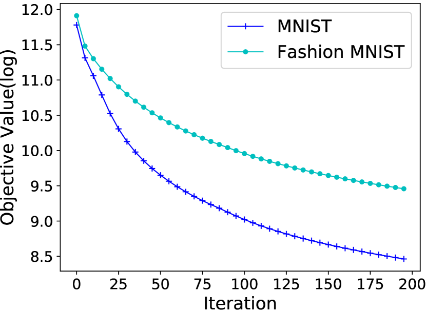
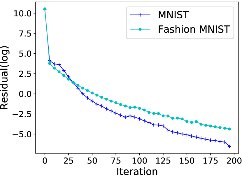
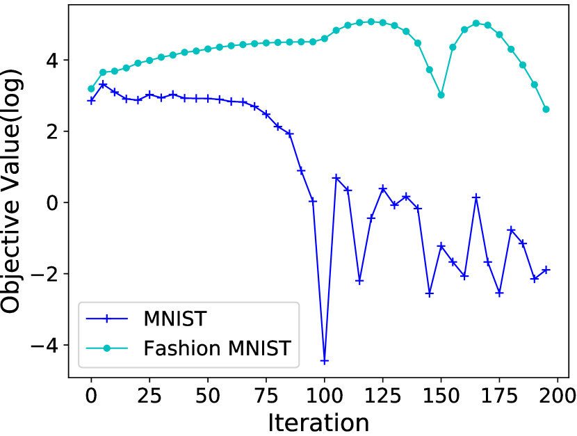
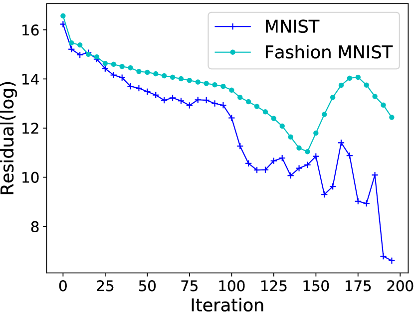
First, we show that our proposed dlADMM algorithm converges when $\rho$ is sufficiently large and diverges when $\rho$ is small for both the MNIST dataset and the Fashion MNIST dataset.
The convergence and divergence of dlADMM algorithm are shown in Figures 2 and 3 when $\rho=1$ and $\rho=10^{-6}$ ,respectively. In Figures 2(a) and 3(a), the X axis and Y axis denote the number of iterations and the logarithm of objective value, respectively. In Figures, 2(b) and 3(b), the X axis and Y axis denote the number of iterations and the logarithm of the residual, respectively. Figure 2, both the objective value and the residual decreased monotonically for the MNIST dataset and the Fashion-MNIST dataset, which validates our theoretical guarantees in Theorem 4.2. Moreover, Figure 3 illustrates that both the objective value and the residual diverge when $\rho=10^{-6}$. The curves fluctuated drastically on the objective value. Even though there was a decreasing trend for the residual, it still fluctuated irregularly and failed to converge.

5.2.2. Performance

(a). Training accuracy

(b). Test accuracy

Figure 4. Performance of all methods for the MNIST dataset: dlADMM algorithm outperformed most of the comparison methods.

(a). Training Accuracy

(b).Test Accuracy

Figure 5. Performance of all methods for the Fashion MNIST dataset: dlADMM algorithm outperformed most of the comparsion methods.

MNIST dataset: From 200 to 1,000 neurons
	200	400	600	800	1000
$10^{-6}$	1.9025	2.7750	3.6615	4.5709	5.7988
$10^{-5}$	2.8778	4.6197	6.3620	8.2563	10.0323
$10^{-4}$	2.2761	3.9745	5.8645	7.6656	9.9221
$10^{-3}$	2.4361	4.3284	6.5651	8.7357	11.3736
$10^{-2}$	2.7912	5.1383	7.8249	10.0300	13.4485
Fashion MNIST dataset: From 200 to 1,000 neurons
	200	400	600	800	1000
$10^{-6}$	2.0069	2.8694	4.0506	5.1438	6.7406
$10^{-5}$	3.3445	5.4190	7.3785	9.0813	11.0531
$10^{-4}$	2.4974	4.3729	6.4257	8.3520	10.0728
$10^{-3}$	2.7108	4.7236	7.1507	9.4534	12.3326
$10^{-2}$	2.9577	5.4173	8.2518	10.0945	14.3465

Table 2. The relationship between running time per iteration (in second) and the number of neurons for each layer as well as value of $\rho$ when the training size was fixed: generally, the running time increased as the number of neurons and the value of $\rho$ became larger.

MNIST dataset: From 11,000 to 55,000 training samples
	11,000	22,000	33,000	44,000	55,000
$10^{-6}$	1.0670	2.0682	3.3089	4.6546	5.7709
$10^{-5}$	2.3981	3.9086	6.2175	7.9188	10.2741
$10^{-4}$	2.1290	3.7891	5.6843	7.7625	9.8843
$10^{-3}$	2.1295	4.1939	6.5039	8.8835	11.3368
$10^{-2}$	2.5154	4.9638	7.6606	10.4580	13.4021
Fashion MNIST dataset: From 12,000 to 60,000 training samples
	12,000	24,000	36,000	48,000	60,000
$10^{-6}$	1.2163	2.3376	3.7053	5.1491	6.7298
$10^{-5}$	2.5772	4.3417	6.6681	8.3763	11.0292
$10^{-4}$	2.3216	4.1163	6.2355	8.3819	10.7120
$10^{-3}$	2.3149	4.5250	6.9834	9.5853	12.3232
$10^{-2}$	2.7381	5.3373	8.1585	11.1992	14.2487

Table 3. The relationship between running time per iteration (in second) and the size of training samples as well as value of $\rho$ when the number of neurons is fixed: generally, the running time increased as the training sample and the value of $\rho$ became larger.

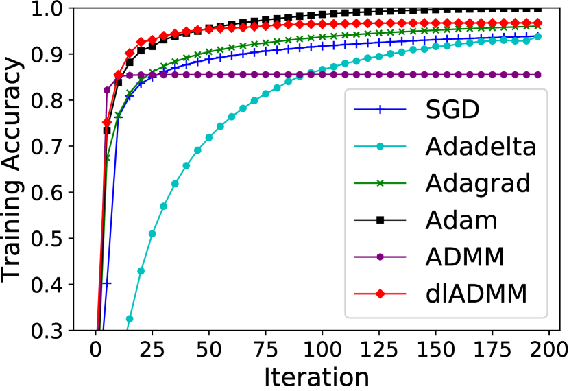
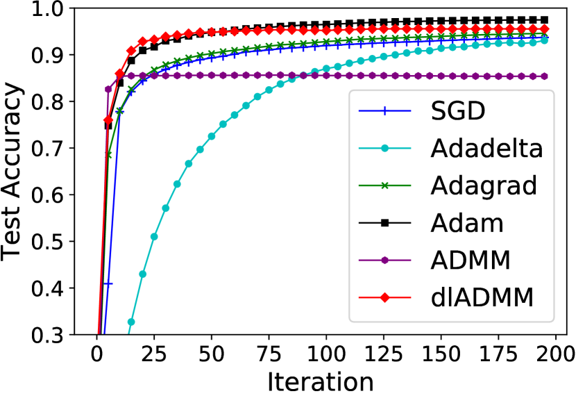
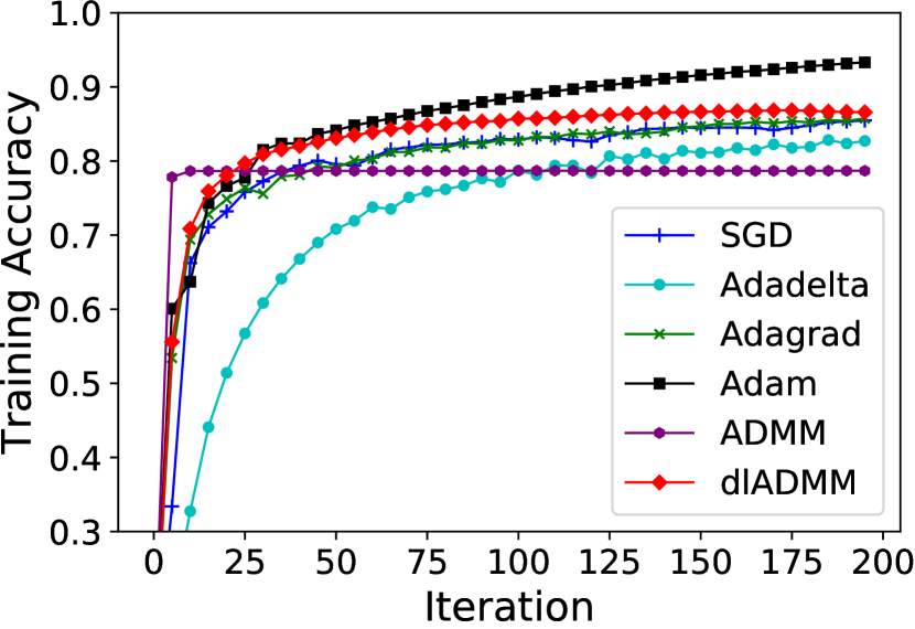
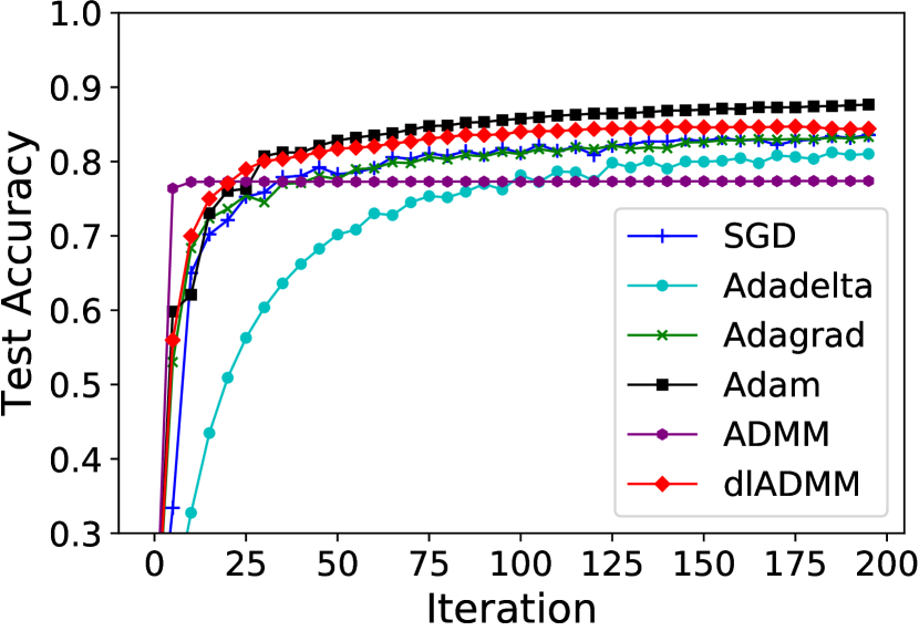
Figure 4 and Figure 5 show the curves of the training accuracy and test accuracy of our proposed dlADMM algorithm and baselines, respectively. Overall, both the training accuracy and the test accuracy of our proposed dlADMM algorithm outperformed most baselines for both the MNIST dataset and the Fashion MNIST dataset. Specifically, the curves of our dlADMM algorithm soared to $0.8$ at the early stage, and then raised steadily towards to $0.9$ or more. The curves of the most SGD-related methods, SGD, Adadelta, and Adagrad, moved more slowly than our proposed dlADMM algorithm. The curves of the ADMM also rocketed to around $0.8$, but decreased slightly later on. Only the state-of-the-art Adam performed better than dlADMM slightly.

5.2.3. Scalability Analysis

In this subsection, the relationship between running time per iteration of our proposed dlADMM algorithm and three potential factors, namely, the value of $\rho$, the size of training samples, and the number of neurons was explored. The running time was calculated by the average of 200 iterations.
Firstly, when the training size was fixed, the computational result for the MNIST dataset and Fashion MNIST dataset is shown in Table 2. The number of neurons for each layer ranged from 200 to 1,000, with an increase of 200 each time. The value of $\rho$ ranged from $10^{-6}$ to $10^{-2}$, with multiplying by 10 each time. Generally, the running time increased as the number of neurons and the value of $\rho$ became larger. However, there were a few exceptions: for example, when there were 200 neurons for the MNIST dataset, and $\rho$ increased from $10^{-5}$ to $10^{-4}$, the running time per iteration dropped from $2.8778$ seconds to $2.2761$ seconds.
Secondly, we fixed the number of neurons for each layer as $1,000$. The relationship between running time per iteration, the training size and the value of $\rho$ is shown in Table 3. The value of $\rho$ ranged from $10^{-6}$ to $10^{-2}$, with multiplying by 10 each time. The training size of the MNIST dataset ranged from $11,000$ to $55,000$, with an increase of $11,000$ each time. The training size of the Fashion MNIST dataset ranged from $12,000$ to $60,000$, with an increase of $12,000$ each time. Similiar to Table 3, the running time increased generally as the training sample and the value of $\rho$ became larger and some exceptions exist.

6. Conclusion and Future Work

Alternating Direction Method of Multipliers (ADMM) is a good alternative to Stochastic Gradient Descent (SGD) for deep learning problems. In this paper, we propose a novel deep learning Alternating Direction Method of Multipliers (dlADMM) to address some previously mentioned challenges. Firstly, the dlADMM updates parameters from backward to forward in order to transmit parameter information more efficiently. The time complexity is successfully reduced from $O(n^{3})$ to $O(n^{2})$ by iterative quadratic approximations and backtracking. Finally, the dlADMM is guaranteed to converge to a critical solution under mild conditions. Experiments on benchmark datasets demonstrate that our proposed dlADMM algorithm outperformed most of the comparison methods.
In the future, we may extend our dlADMM from the fully-connected neural network to the famous Convolutional Neural Network (CNN) or Recurrent Neural Network (RNN), because our convergence guarantee is also applied to them. We also consider other nonlinear activation functions such as sigmoid and hyperbolic tangent function (tanh).

Supplementary Materials

Appendix A Algorithms to update $W^{k+1}_{l}$ and $a^{k+1}_{l}$

The algorithms to update $W^{k+1}_{l}$ and $a^{k+1}_{l}$ are described in the Algorithms 4 and 5, respectively.

Algorithm 4 The Backtracking Algorithm to update ${W}^{k+1}_{l}$

0:  ${\textbf{W}}^{k+1}_{l-1}$,${\textbf{b}}^{k+1}_{l-1}$, ${\textbf{z}}^{k+1}_{l-1}$,${\textbf{a}}^{k+1}_{l-1}$,$u^{k}$, $\rho$, some constant ${\gamma}>1$.

0:  ${\theta}^{k+1}_{l}$,${{W}}^{k+1}_{l}$.

1:  Pick up ${\alpha}$ and ${\zeta}=\overline{W}^{k+1}_{l}-\nabla_{\overline{W}^{k+1}_{l}}\phi/{\alpha}$.

2:  while $\phi(\{W^{k+1}_{i}\}_{i=1}^{l-1},{\zeta},\{\overline{W}^{k+1}_{i}\}_{i=l+1}^{L},{\textbf{b}}^{k+1}_{l},{\textbf{z}}^{k+1}_{l},{\textbf{a}}^{k+1}_{l},u^{k})>{P}_{l}({\zeta};{\alpha})$ do

3:    ${\alpha}\leftarrow{\alpha}\ {\gamma}$.

4:    Solve ${\zeta}$ by Equation (11).

5:  end while

6:  Output ${\theta}^{k+1}_{l}\leftarrow{\alpha}$.

7:  Output ${W}^{k+1}_{l}\leftarrow{\zeta}$.

Algorithm 5 The Backtracking Algorithm to update ${a}^{k+1}_{l}$

0:  ${\textbf{W}}^{k+1}_{l}$,${\textbf{b}}^{k+1}_{l}$, ${\textbf{z}}^{k+1}_{l}$,${\textbf{a}}^{k+1}_{l-1}$,$u^{k}$, $\rho$, some constant ${\eta}>1$.

0:  ${\tau}^{k+1}_{l}$,${{a}}^{k+1}_{l}$.

1:  Pick up ${t}$ and ${\beta}=\overline{a}^{k+1}_{l}-\nabla_{\overline{a}^{k+1}_{l}}\phi/{t}$

2:  while $\phi({\textbf{W}}^{k+1}_{l+1},{\textbf{b}}^{k+1}_{l+1},{\textbf{z}}^{k+1}_{l+1},\{a^{k+1}_{i}\}_{i=1}^{l-1},{\beta},\{\overline{a}^{k+1}_{i}\}_{i=l+1}^{L-1},u^{k})>{Q}_{l}({\beta};{t})$ do

3:    ${t}\leftarrow{t}{\eta}$.

4:    ${\beta}\leftarrow\overline{a}^{k+1}_{l}-\nabla_{\overline{a}^{k+1}_{l}}\phi/{t}$.

5:  end while

6:  Output ${\tau}^{k+1}_{l}\leftarrow{t}$.

7:  Output ${a}^{k+1}_{l}\leftarrow{\beta}$.

Appendix B Lemmas for the Proofs of Properties

The following several lemmas are preliminary results.

Lemma B.1.

Equation (9) holds if and only if there exists $\overline{s}\in\partial\Omega_{l}(\overline{W}^{k+1}_{l})$, the subgradient of $\Omega_{l}(\overline{W}^{k+1}_{l})$ such that

$$\nabla_{{W}^{k}_{l}}\phi({\overline{\textbf{W}}}^{k+1}_{l+1},\overline{\textbf{b}}^{k+1}_{l},\overline{\textbf{z}}^{k+1}_{l},\overline{\textbf{a}}^{k+1}_{l},u^{k})+\overline{\theta}^{k+1}_{l}\circ(\overline{W}^{k+1}_{l}-{W}^{k}_{l})+\overline{s}=0$$

Likewise, Equation (11) holds if and only if there exists $s\in\partial\Omega_{l}(W^{k+1}_{l})$, the subgradient of $\Omega_{l}(W^{k+1}_{l})$ such that

$$\nabla_{\overline{W}^{k+1}_{l}}\phi({\textbf{W}}^{k+1}_{l-1},\textbf{b}^{k+1}_{l-1},\textbf{z}^{k+1}_{l-1},{\textbf{a}}^{k+1}_{l-1},u^{k})+\theta^{k+1}_{l}\circ(W^{k+1}_{l}-\overline{W}^{k+1}_{l})+s=0$$

Proof.

These can be obtained by directly applying the optimality conditions of Equation (9) and Equation (11), respectively. ∎

Lemma B.2.

$\nabla_{z_{L}^{k}}R(z_{L}^{k};y)+u^{k}=0$ for all $k\in\mathbb{N}$.

Proof.

The optimality condition of $z^{k}_{L}$ in Equation (15) gives rise to

$$\nabla_{z^{k}_{L}}R(z^{k}_{L};y)+\rho(z^{k}_{L}-W^{k}_{L}a^{k}_{L-1}-b^{k}_{L})+u^{k-1}=0$$

Because $u^{k}=u^{k-1}+\rho(z^{k}_{L}-W^{k}_{L}a^{k}_{L-1}-b^{k}_{L})$, then we have $\nabla_{z_{L}^{k}}R(z_{L}^{k};y)+u^{k}=0$. ∎

Lemma B.3.

It holds that $\forall z_{L,1},z_{L,2}\in\mathbb{R}^{n_{L}}$,

$$R(z_{L,1};y)\leq R(z_{L,2};y)+\nabla_{z_{L,2}}R^{T}(z_{L,2};y)(z_{L,1}-z_{L,2})+(H/2)\|z_{L,1}-z_{L,2}\|^{2}$$

$$-R(z_{L,1};y)\leq-R(z_{L,2};y)-\nabla_{z_{L,2}}R^{T}(z_{L,2};y)(z_{L,1}-z_{L,2})+(H/2)\|z_{L,1}-z_{L,2}\|^{2}$$

Proof.

Because $R(z_{L};y)$ is Lipschitz differentiable by Assumption 2, so is $-R(z_{L};y)$. Therefore, this lemma is proven exactly as same as Lemma 2.1 in [1]. ∎

Lemma B.4.

For Equations (6) and (12), if $\overline{B},B\geq\nu$,then the following inequalities hold:

(19) $$\overline{U}_{l}(\overline{\textbf{b}}^{k+1}_{l};\overline{B})\geqslant\phi(\overline{\textbf{W}}^{k+1}_{l+1},\overline{\textbf{b}}^{k+1}_{l},\overline{\textbf{z}}^{k+1}_{l},\overline{\textbf{a}}^{k+1}_{l},u^{k})$$

(20) $$U_{l}(\textbf{b}^{k+1}_{l};B)\geqslant\phi(\textbf{W}^{k+1}_{l},\textbf{b}^{k+1}_{l},\textbf{z}^{k+1}_{l-1},\textbf{a}^{k+1}_{l-1},u^{k})$$

Proof.

Because $\phi(\textbf{W},\textbf{b},\textbf{z},\textbf{a},u)$ is Lipschitz differentiable with respect to b with Lipschitz coefficient $\nu$ (the definition of Lipschitz differentiablity can be found in [1]), we directly apply Lemma 2.1 in [1] to $\phi$ to obtain Equations (19) and (20), respectively. ∎

Lemma B.5.

It holds that for $\forall k\in\mathbb{N}$,

(21) $$L_{\rho}(\overline{\textbf{W}}^{k+1}_{l+1},\overline{\textbf{b}}^{k+1}_{l+1},\overline{\textbf{z}}^{k+1}_{l+1},\overline{\textbf{a}}^{k+1}_{l+1},u^{k})-L_{\rho}(\overline{\textbf{W}}^{k+1}_{l+1},\overline{\textbf{b}}^{k+1}_{l+1},\overline{\textbf{z}}^{k+1}_{l+1},\overline{\textbf{a}}^{k+1}_{l},u^{k})\geq\|\overline{\tau}_{l}^{k+1}\circ(\overline{a}^{k+1}_{l}-a_{l}^{k})^{\circ 2}\|_{1}/2(l=1,\cdots,L-1)$$

(22) $$L_{\rho}(\overline{\textbf{W}}^{k+1}_{l+1},\overline{\textbf{b}}^{k+1}_{l+1},\overline{\textbf{z}}^{k+1}_{l+1},\overline{\textbf{a}}^{k+1}_{l},u^{k})\geq L_{\rho}(\overline{\textbf{W}}^{k+1}_{l+1},\overline{\textbf{b}}^{k+1}_{l+1},\overline{\textbf{z}}^{k+1}_{l},\overline{\textbf{a}}^{k+1}_{l},u^{k})(l=1,\cdots,L-1)$$

(23) $$L_{\rho}({\textbf{W}}^{k},{\textbf{b}}^{k},{\textbf{z}}^{k},{\textbf{a}}^{k},u^{k})-L_{\rho}({\textbf{W}}^{k},{\textbf{b}}^{k},\overline{\textbf{z}}^{k+1}_{L},{\textbf{a}}^{k},u^{k})\geq(\rho/2)\|\overline{z}^{k+1}_{L}-z^{k}_{L}\|^{2}_{2}$$

(24) $$L_{\rho}(\overline{\textbf{W}}^{k+1}_{l+1},\overline{\textbf{b}}^{k+1}_{l+1},\overline{\textbf{z}}^{k+1}_{l},\overline{\textbf{a}}^{k+1}_{l},u^{k})-L_{\rho}(\overline{\textbf{W}}^{k+1}_{l+1},\overline{\textbf{b}}^{k+1}_{l},\overline{\textbf{z}}^{k+1}_{l},\overline{\textbf{a}}^{k+1}_{l},u^{k})\geq(\nu/2)\|\overline{b}^{k+1}_{l}-b_{l}^{k}\|^{2}_{2}(l=1,\cdots,L-1)$$

(25) $$L_{\rho}({\textbf{W}}^{k},{\textbf{b}}^{k},\overline{\textbf{z}}^{k+1}_{L},{\textbf{a}}^{k},u^{k})-L_{\rho}({\textbf{W}}^{k},\overline{\textbf{b}}^{k+1}_{L},\overline{\textbf{z}}^{k+1}_{L},{\textbf{a}}^{k},u^{k})\geq(\rho/2)\|\overline{b}^{k+1}_{L}-b^{k}_{L}\|^{2}_{2}$$

(26) $$L_{\rho}(\overline{\textbf{W}}^{k+1}_{l+1},\overline{\textbf{b}}^{k+1}_{l},\overline{\textbf{z}}^{k+1}_{l},\overline{\textbf{a}}^{k+1}_{l},u^{k})-L_{\rho}(\overline{\textbf{W}}^{k+1}_{l},\overline{\textbf{b}}^{k+1}_{l},\overline{\textbf{z}}^{k+1}_{l},\overline{\textbf{a}}^{k+1}_{l},u^{k})\geq\|\overline{\theta}_{l}^{k+1}\circ(\overline{W}^{k+1}_{l}-W_{l}^{k})^{\circ 2}\|_{1}/2(l=1,\cdots,L)$$

(27) $$L_{\rho}({\textbf{W}}^{k+1}_{l-1},{\textbf{b}}^{k+1}_{l-1},{\textbf{z}}^{k+1}_{l-1},{\textbf{a}}^{k+1}_{l-1},u^{k})-L_{\rho}({\textbf{W}}^{k+1}_{l},{\textbf{b}}^{k+1}_{l-1},{\textbf{z}}^{k+1}_{l-1},{\textbf{a}}^{k+1}_{l-1},u^{k})\geq\|{\theta}_{l}^{k+1}\circ({W}^{k+1}_{l}-\overline{W}_{l}^{k+1})^{\circ 2}\|_{1}/2(l=1,\cdots,L)$$

(28) $$L_{\rho}({\textbf{W}}^{k+1}_{l},{\textbf{b}}^{k+1}_{l-1},{\textbf{z}}^{k+1}_{l-1},{\textbf{a}}^{k+1}_{l-1},u^{k})-L_{\rho}({\textbf{W}}^{k+1}_{l},{\textbf{b}}^{k+1}_{l},{\textbf{z}}^{k+1}_{l-1},{\textbf{a}}^{k+1}_{l-1},u^{k})\geq(\nu/2)\|{b}^{k+1}_{l}-\overline{b}_{l}^{k+1}\|^{2}_{2}(l=1,\cdots,L-1)$$

(29) $$L_{\rho}({\textbf{W}}^{k+1},{\textbf{b}}^{k+1}_{L-1},{\textbf{z}}^{k+1}_{L-1},{\textbf{a}}^{k+1},u^{k})-L_{\rho}({\textbf{W}}^{k+1},{\textbf{b}}^{k+1},{\textbf{z}}^{k+1}_{L-1},{\textbf{a}}^{k+1},u^{k})\geq(\rho/2)\|{b}^{k+1}_{L}-\overline{b}_{L}^{k+1}\|^{2}_{2}$$

(30) $$L_{\rho}({\textbf{W}}^{k+1}_{l},{\textbf{b}}^{k+1}_{l},{\textbf{z}}^{k+1}_{l-1},{\textbf{a}}^{k+1}_{l-1},u^{k})\geq L_{\rho}({\textbf{W}}^{k+1}_{l},{\textbf{b}}^{k+1}_{l},{\textbf{z}}^{k+1}_{l},{\textbf{a}}^{k+1}_{l-1},u^{k})(l=1,\cdots,L-1)$$

(31) $$L_{\rho}({\textbf{W}}^{k+1}_{l},{\textbf{b}}^{k+1}_{l},{\textbf{z}}^{k+1}_{l},{\textbf{a}}^{k+1}_{l-1},u^{k})-L_{\rho}({\textbf{W}}^{k+1}_{l},{\textbf{b}}^{k+1}_{l},{\textbf{z}}^{k+1}_{l},{\textbf{a}}^{k+1}_{l},u^{k})\geq\|{\tau}_{l}^{k+1}\circ({a}^{k+1}_{l}-\overline{a}_{l}^{k+1})^{\circ 2}\|_{1}/2(l=1,\cdots,L-1)$$

Proof.

Essentially, all inequalities can be obtained by applying optimality conditions of updating $\overline{a}^{k+1}_{l}$, $\overline{z}^{k+1}_{l}$, $\overline{b}^{k+1}_{l}$, $\overline{W}^{k+1}_{l}$, ${W}^{k+1}_{l}$, ${b}^{k+1}_{l}$, ${z}^{k+1}_{l}$ and ${a}^{k+1}_{l}$, respectively. We only prove Inequality (23), (27), (28) and (30) .This is because Inequalities (21), (26) and (31) follow the routine of Inequality (27), Inequalities (24), (25) and (29) follow the routine of Inequality (28), and Inequality (22) follows the routine of Inequality (30).
Firstly, we focus on Inequality (23).

$$L_{\rho}({\textbf{W}}^{k},{\textbf{b}}^{k},{\textbf{z}}^{k},{\textbf{a}}^{k},u^{k})-L_{\rho}({\textbf{W}}^{k},{\textbf{b}}^{k},\overline{\textbf{z}}^{k+1}_{L},{\textbf{a}}^{k},u^{k})$$

$$=R(z^{k}_{L};y)+(u^{k})^{T}(z^{k}_{L}-W^{k}_{L}a^{k}_{L-1}-b^{k}_{L})+(\rho/2)\|z^{k}_{L}-W^{k}_{L}a^{k}_{L-1}-b^{k}_{L}\|^{2}_{2}$$

$$-R(\overline{z}^{k+1}_{L};y)-(u^{k})^{T}(\overline{z}^{k+1}_{L}-W^{k}_{L}a^{k}_{L-1}-b^{k}_{L})-(\rho/2)\|\overline{z}^{k+1}_{L}-W^{k}_{L}a^{k}_{L-1}-b^{k}_{L}\|^{2}_{2}$$

$$=R(z^{k}_{L};y)-R(\overline{z}^{k+1}_{L};y)+(u^{k})^{T}(z^{k}_{L}-\overline{z}^{k+1}_{L})+(\rho/2)\|\overline{z}^{k+1}_{L}-z^{k}_{L}\|^{2}_{2}$$

(32) $$+\rho(\overline{z}^{k+1}_{L}-W^{k}_{L}a^{k}_{L-1}-b^{k}_{L})^{T}(z^{k}_{L}-\overline{z}^{k+1}_{L})$$

where the second equality follows from the cosine rule $\|z^{k}_{L}-W^{k}_{L}a^{k}_{L-1}-b^{k}_{L}\|^{2}_{2}-\|\overline{z}^{k+1}_{L}-W^{k}_{L}a^{k}_{L-1}-b^{k}_{L}\|^{2}_{2}=\|\overline{z}^{k+1}_{L}-z^{k}_{L}\|^{2}_{2}+(\overline{z}^{k+1}_{L}-W^{k}_{L}a^{k}_{L-1}-b^{k}_{L})^{T}(z^{k}_{L}-\overline{z}^{k+1}_{L})$.
According to the optimality condition of Equation (5), we have $\nabla_{\overline{z}^{k+1}_{L}}R(\overline{z}^{k+1}_{L};y)+u^{k}+\rho(\overline{z}^{k+1}_{L}-W^{k}_{L}a^{k}_{L-1}-b^{k}_{L})=0$. Because $R(z_{L};y)$ is convex and differentiable with regard to $z_{L}$, its subgradient is also its gradient. According to the definition of subgradient, we have

$$R(z^{k}_{L};y) \geq R(\overline{z}^{k+1}_{L};y)+\nabla_{\overline{z}^{k+1}_{L}}R^{T}(\overline{z}^{k+1}_{L};y)(z^{k}_{L}-\overline{z}^{k+1}_{L})$$

(33) $$=R(\overline{z}^{k+1}_{L};y)-(u^{k}+\rho(\overline{z}^{k+1}_{L}-W^{k}_{L}a^{k}_{L-1}-b^{k}_{L}))^{T}(z^{k}_{L}-\overline{z}^{k+1}_{L})$$

We introduce Equation (33) into Equation (32) to obtain Equation (23).
Secondly, we focus on Inequality (27). The stopping criterion of Algorithm 4 shows that

(34) $$\phi(\textbf{W}^{k+1}_{l},\textbf{b}^{k+1}_{l-1},\textbf{z}^{k+1}_{l-1},\textbf{a}^{k+1}_{l-1},u^{k})\leq P_{l}(W^{k+1}_{l};\theta^{k+1}_{l}).$$

Because $\Omega_{W_{l}}(W_{l})$ is convex, according to the definition of subgradient, we have

(35) $$\Omega_{l}(\overline{W}^{k+1}_{l})\geq\Omega_{l}({W}^{k+1}_{l})+s^{T}(\overline{W}_{l}^{k+1}-W_{l}^{k+1}).$$

where $s$ is defined in the premise of Lemma B.1. Therefore, we have

$$L_{\rho}({\textbf{W}}^{k+1}_{l-1},{\textbf{b}}^{k+1}_{l-1},{\textbf{z}}^{k+1}_{l-1},{\textbf{a}}^{k+1}_{l-1},u^{k})-L_{\rho}({\textbf{W}}^{k+1}_{l},{\textbf{b}}^{k+1}_{l-1},{\textbf{z}}^{k+1}_{l-1},{\textbf{a}}^{k+1}_{l-1},u^{k})$$

$$=\phi({\textbf{W}}^{k+1}_{l-1},{\textbf{b}}^{k+1}_{l-1},{\textbf{z}}^{k+1}_{l-1},{\textbf{a}}^{k+1}_{l-1},u^{k})+\Omega_{l}(\overline{W}^{k+1}_{l})-\phi({\textbf{W}}^{k+1}_{l},{\textbf{b}}^{k+1}_{l-1},{\textbf{z}}^{k+1}_{l-1},{\textbf{a}}^{k+1}_{l-1},u^{k})-\Omega_{l}(W^{k+1}_{l})\ \text{(Definition of $L_{\rho}$)}$$

$$\geq\Omega_{l}(\overline{W}^{k+1}_{l})-\Omega_{l}(W^{k+1}_{l})-\nabla\phi^{T}_{\overline{W}^{k+1}_{l}}(W^{k+1}_{l}-\overline{W}^{k+1}_{l})-\|\theta_{l}^{k+1}\circ(W^{k+1}_{l}-\overline{W}_{l}^{k+1})^{\circ 2}\|_{1}/2(\text{Equation \eqref{ineq:ineq1}})$$

$$\geq s^{T}(\overline{W}^{k+1}_{l}-{W}^{k+1}_{l})-\nabla\phi^{T}_{\overline{W}^{k+1}_{l}}(W^{k+1}_{l}-\overline{W}^{k+1}_{l})-\|\theta_{l}^{k+1}\circ(W^{k+1}_{l}-\overline{W}_{l}^{k+1})^{\circ 2}\|_{1}/2(\text{Equation \eqref{ineq:ineq2}})$$

$$=(s^{T}+\nabla\phi^{T}_{\overline{W}^{k+1}_{l}})(\overline{W}^{k+1}_{l}-W^{k+1}_{l})-\|\theta_{l}^{k+1}\circ(W^{k+1}_{l}-\overline{W}_{l}^{k+1})^{\circ 2}\|_{1}/2$$

$$=\|\theta_{l}^{k+1}\circ(W^{k+1}_{l}-\overline{W}_{l}^{k+1})^{\circ 2}\|_{1}/2\ (\text{Lemma \ref{lemma:lemma 1}}).$$

Thirdly, we focus on Inequality (28).

$$L_{\rho}({\textbf{W}}^{k+1}_{l},{\textbf{b}}^{k+1}_{l-1},{\textbf{z}}^{k+1}_{l-1},{\textbf{a}}^{k+1}_{l-1},u^{k})-L_{\rho}({\textbf{W}}^{k+1}_{l},{\textbf{b}}^{k+1}_{l},{\textbf{z}}^{k+1}_{l-1},{\textbf{a}}^{k+1}_{l-1},u^{k})$$

$$=\phi({\textbf{W}}^{k+1}_{l},{\textbf{b}}^{k+1}_{l-1},{\textbf{z}}^{k+1}_{l-1},{\textbf{a}}^{k+1}_{l-1},u^{k})-\phi({\textbf{W}}^{k+1}_{l},{\textbf{b}}^{k+1}_{l},{\textbf{z}}^{k+1}_{l-1},{\textbf{a}}^{k+1}_{l-1},u^{k})$$

$$\geq(\nu/2)\|{b}^{k+1}_{l}-\overline{b}_{l}^{k+1}\|^{2}_{2}.(\text{Lemma \ref{lemma:lemma 2}})$$

Finally, we focus on Equation (30). This follows directly from the optimality of $z^{k+1}_{l}$ in Equation (14). ∎

Lemma B.6.

If $\rho>2H$ so that $C_{1}=\rho/2-H/2-H^{2}/\rho>0$, then it holds that

$$L_{\rho}(\textbf{W}^{k+1},\textbf{b}^{k+1},\textbf{z}^{k+1}_{L-1},\textbf{a}^{k+1},u^{k})-L_{\rho}(\textbf{W}^{k+1},\textbf{b}^{k+1},\textbf{z}^{k+1},\textbf{a}^{k+1},u^{k+1})$$

(36) $$\geq C_{1}\|z_{L}^{k+1}-\overline{z}_{L}^{k+1}\|^{2}_{2}-(H^{2}/\rho)\|\overline{z}_{L}^{k+1}-{z}_{L}^{k}\|^{2}_{2}.$$

Proof.

$$L_{\rho}(\textbf{W}^{k+1},\textbf{b}^{k+1},\textbf{z}^{k+1}_{L-1},\textbf{a}^{k+1},u^{k})-L_{\rho}(\textbf{W}^{k+1},\textbf{b}^{k+1},\textbf{z}^{k+1},\textbf{a}^{k+1},u^{k+1})$$

$$=R(\overline{z}_{L}^{k+1};y)-R({z}_{L}^{k+1};y)+(u^{k+1})^{T}(\overline{z}_{L}^{k+1}-z_{L}^{k+1})+(\rho/2)\|z_{L}^{k+1}-\overline{z}_{L}^{k+1}\|^{2}_{2}-(1/\rho)\|u^{k+1}-u^{k}\|^{2}_{2}$$

$$=R(\overline{z}_{L}^{k+1};y)-R(z_{L}^{k+1};y)+\nabla_{z_{L}^{k+1}}R(z_{L}^{k+1};y)^{T}(z_{L}^{k+1}-\overline{z}_{L}^{k+1})+(\rho/2)\|z_{L}^{k+1}-\overline{z}_{L}^{k+1}\|^{2}_{2}-(1/\rho)\|u^{k+1}-u^{k}\|^{2}_{2}\text{( Lemma \ref{lemma:z_l optimality})}$$

$$\geq(-H/2)\|z_{L}^{k+1}-\overline{z}_{L}^{k+1}\|^{2}_{2}+(\rho/2)\|z_{L}^{k+1}-\overline{z}_{L}^{k+1}\|^{2}_{2}-(1/\rho)\|\nabla_{z_{L}^{k+1}}R(z_{L}^{k+1};y)-\nabla_{z_{L}^{k}}R(z_{L}^{k};y)\|^{2}_{2}$$

($$-R(z_{L};y)$$ is Lipschitz differentiable, Lemmas B.2 and B.3)

$$\geq(-H/2)\|z_{L}^{k+1}-\overline{z}_{L}^{k+1}\|^{2}_{2}+(\rho/2)\|z_{L}^{k+1}-\overline{z}_{L}^{k+1}\|^{2}_{2}-(H^{2}/\rho)\|z_{L}^{k+1}-{z}_{L}^{k}\|^{2}_{2}\text{(Assumption \ref{ass:assumption 2})}$$

$$\geq(-H/2)\|z_{L}^{k+1}-\overline{z}_{L}^{k+1}\|^{2}_{2}+(\rho/2)\|z_{L}^{k+1}-\overline{z}_{L}^{k+1}\|^{2}_{2}-(H^{2}/\rho)\|z_{L}^{k+1}-\overline{z}_{L}^{k+1}\|^{2}_{2}-(H^{2}/\rho)\|\overline{z}_{L}^{k+1}-{z}_{L}^{k}\|^{2}_{2}\text{(triangle inequality)}$$

$$=C_{1}\|z_{L}^{k+1}-\overline{z}_{L}^{k+1}\|^{2}_{2}-(H^{2}/\rho)\|\overline{z}_{L}^{k+1}-{z}_{L}^{k}\|^{2}_{2}.$$

We choose $\rho>2H$ to make $C_{1}>0$. ∎

Appendix C Proof of Theorem 4.1

Proving Theorem 4.1 is equal to proving jointly Theorem C.1, C.2, and C.3, which are elaborated in the following.

Theorem C.1.

Given that Assumptions 1 and 2 hold, the dlADMM satisfies Property 1.

Proof.

There exists $z_{L}^{{}^{\prime}}$ such that $z_{L}^{{}^{\prime}}-W^{k}_{L}a^{k}_{L-1}-b^{k}_{L}=0$. By Assumption 2, we have

$$F(\textbf{W}^{k},\textbf{b}^{k},\{z_{l}^{k}\}_{l=1}^{L-1},z^{{}^{\prime}}_{L},\textbf{a}^{k})\geq\min S>-\infty$$

where $S=\{F(\textbf{W},\textbf{b},\textbf{z},\textbf{a}):z_{L}-W_{L}a_{L-1}-b_{L}=0\}$. Then we have

$$L_{\rho}(\textbf{W}^{k},\textbf{b}^{k},\textbf{z}^{k},\textbf{a}^{k},u^{k})$$

$$=F(\textbf{W}^{k},\textbf{b}^{k},\textbf{z}^{k},\textbf{a}^{k})+(u^{k})^{T}(z^{k}_{L}-W^{k}_{L}a^{k}_{L-1}-b^{k}_{L})+(\rho/2)\|z^{k}_{L}-W^{k}_{L}a^{k}_{L-1}-b^{k}_{L}\|^{2}_{2}$$

$$=F(\textbf{W}^{k},\textbf{b}^{k},\textbf{z}^{k},\textbf{a}^{k})+(u^{k})^{T}(z^{k}_{L}-z^{{}^{\prime}}_{L})+(\rho/2)\|z^{k}_{L}-W^{k}_{L}a^{k}_{L-1}-b^{k}_{L}\|^{2}_{2}\ \text{$(z_{L}^{{}^{\prime}}-W^{k}_{L}a^{k}_{L-1}-b^{k}_{L}=0)$}$$

$$=F(\textbf{W}^{k},\textbf{b}^{k},\textbf{z}^{k},\textbf{a}^{k})+\nabla_{z^{k}_{L}}R^{T}(z^{k}_{L};y)(z^{{}^{\prime}}_{L}-z^{k}_{L})+(\rho/2)\|z^{k}_{L}-W^{k}_{L}a^{k}_{L-1}-b^{k}_{L}\|^{2}_{2}\text{(Lemma \ref{lemma:z_l optimality})}$$

$$=\sum\nolimits_{l=1}^{L}\Omega_{l}(W^{k}_{l})+(\nu/2)\sum\nolimits_{l=1}^{L-1}(\|z^{k}_{l}-W^{k}_{l}a^{k}_{l-1}-b^{k}_{l}\|^{2}_{2}+\|a^{k}_{l}-f(z^{k}_{l})\|^{2}_{2})+R(z^{k}_{L};y)+\nabla_{z^{k}_{L}}R^{T}(z^{k}_{L};y)(z^{{}^{\prime}}_{L}-z^{k}_{L})$$

$$+(\rho/2)\|z^{k}_{L}-W^{k}_{L}a^{k}_{L-1}-b^{k}_{L}\|^{2}_{2}\text{(The definition of $F$)}$$

$$\geq\sum\nolimits_{l=1}^{L}\Omega_{l}(W^{k}_{l})+(\nu/2)\sum\nolimits_{l=1}^{L-1}(\|z^{k}_{l}-W^{k}_{l}a^{k}_{l-1}-b^{k}_{l}\|^{2}_{2}+\|a^{k}_{l}-f(z^{k}_{l})\|^{2}_{2})+R(z^{{}^{\prime}}_{L};y)+(\rho-H/2)\|z^{k}_{L}-W^{k}_{L}a^{k}_{L-1}-b^{k}_{L}\|^{2}_{2}$$

(Lemmas B.2 and B.3, $$R(z_{L};y)$$ is Lipschitz differentiable)

$$>-\infty$$

It concludes from Lemma B.5 and Lemma B.6 that $L_{\rho}(\textbf{W}^{k},\textbf{b}^{k},\textbf{z}^{k},\textbf{a}^{k},u^{k})$ is upper bounded by $L_{\rho}(\textbf{W}^{0},\textbf{b}^{0},\textbf{z}^{0},\textbf{a}^{0},\textbf{u}^{0})$ and so are $\sum\nolimits_{l=1}^{L}\Omega_{l}(W^{k}_{l})+(\nu/2)\sum\nolimits_{l=1}^{L-1}(\|z^{k}_{l}-W^{k}_{l}a^{k}_{l-1}-b^{k}_{l}\|^{2}_{2}+\|a^{k}_{l}-f(z^{k}_{l})\|^{2}_{2})$ and $\|z^{k}_{L}-W^{k}_{L}a^{k}_{L-1}-b^{k}_{L}\|^{2}_{2}$. By Assumption 2, $(\textbf{W}^{k},\textbf{b}^{k},\textbf{z}^{k},\textbf{a}^{k})$ is bounded. By Lemma B.2, it is obvious that $u^{k}$ is bounded as well. ∎

Theorem C.2.

Given that Assumptions 1 and 2 hold, the dlADMM satisfies Property 2.

Proof.

This follows directly from Lemma B.5 and Lemma B.6. ∎

Theorem C.3.

Given that Assumptions 1 and 2 hold, the dlADMM satisfies Property 3.

Proof.

We know that

$$\partial L_{\rho}(\textbf{W}^{k+1},\textbf{b}^{k+1},\textbf{z}^{k+1},\textbf{a}^{k+1},u^{k+1})$$

$$=(\partial_{\textbf{W}^{k+1}}L_{\rho},\nabla_{\textbf{b}^{k+1}}L_{\rho},\partial_{\textbf{z}^{k+1}}L_{\rho},\nabla_{\textbf{a}^{k+1}}L_{\rho},\nabla_{u^{k+1}}L_{\rho})$$

where $\partial_{\textbf{W}^{k+1}}L_{\rho}=\{\partial_{{W_{l}}^{k+1}}L_{\rho}\}_{l=1}^{L}$, $\nabla_{\textbf{b}^{k+1}}L_{\rho}=\{\nabla_{{b_{l}}^{k+1}}L_{\rho}\}_{l=1}^{L}$, $\partial_{\textbf{z}^{k+1}}L_{\rho}=\{\partial_{{z_{l}}^{k+1}}L_{\rho}\}_{l=1}^{L}$, and $\nabla_{\textbf{a}^{k+1}}L_{\rho}=\{\nabla_{{a_{l}}^{k+1}}L_{\rho}\}_{l=1}^{L-1}$ . To prove Property 3, we need to give an upper bound of $\partial_{\textbf{W}^{k+1}}L_{\rho},\nabla_{\textbf{b}^{k+1}}L_{\rho},\partial_{\textbf{z}^{k+1}}L_{\rho},\nabla_{\textbf{a}^{k+1}}L_{\rho}$ and $\nabla_{u^{k+1}}L_{\rho}$ by a linear combination of $\|\textbf{W}^{k+1}-\overline{\textbf{W}}^{k+1}\|$, $\|\textbf{b}^{k+1}-\overline{\textbf{b}}^{k+1}\|$, $\|\textbf{z}^{k+1}-\overline{\textbf{z}}^{k+1}\|$, $\|\textbf{a}^{k+1}-\overline{\textbf{a}}^{k+1}\|$ and $\|\textbf{z}_{l}^{k+1}-\textbf{z}_{l}^{k}\|$.
For $W^{k+1}_{l}(l<L)$,

$$\partial_{W^{k+1}_{l}}L_{\rho} =\partial\Omega_{l}(W^{k+1}_{l})+\nabla_{W_{l}^{k+1}}\phi(\textbf{W}^{k+1},\textbf{b}^{k+1},\textbf{z}^{k+1},\textbf{a}^{k+1},u^{k+1})$$

$$=\partial\Omega_{l}(W^{k+1}_{l})+\nu(W^{k+1}_{l}a^{k+1}_{l-1}+b^{k+1}_{l}-z^{k+1}_{l})(a^{k+1}_{l-1})^{T}$$

$$=\partial\Omega_{l}(W^{k+1}_{l})+\nabla_{W_{l}^{k+1}}\phi(\textbf{W}^{k+1}_{l},\textbf{b}^{k+1}_{l},\textbf{z}^{k+1}_{l},\textbf{a}^{k+1}_{l-1},u^{k})$$

$$=\partial\Omega_{l}(W^{k+1}_{l})+\nabla_{\overline{W}_{l}^{k+1}}\phi(\textbf{W}^{k+1}_{l-1},\textbf{b}^{k+1}_{l-1},\textbf{z}^{k+1}_{l-1},\textbf{a}^{k+1}_{l-1},u^{k})+\theta^{k+1}_{l}\circ(W^{k+1}_{l}-\overline{W}^{k+1}_{l})-\theta^{k+1}_{l}\circ(W^{k+1}_{l}-\overline{W}^{k+1}_{l})$$

$$-\nabla_{\overline{W}_{l}^{k+1}}\phi(\textbf{W}^{k+1}_{l-1},\textbf{b}^{k+1}_{l-1},\textbf{z}^{k+1}_{l-1},\textbf{a}^{k+1}_{l-1},u^{k})+\nabla_{W_{l}^{k+1}}\phi(\textbf{W}^{k+1}_{l},\textbf{b}^{k+1}_{l},\textbf{z}^{k+1}_{l},\textbf{a}^{k+1}_{l-1},u^{k})$$

$$=\partial\Omega_{l}(W^{k+1}_{l})+\nabla_{\overline{W}_{l}^{k+1}}\phi(\textbf{W}^{k+1}_{l-1},\textbf{b}^{k+1}_{l-1},\textbf{z}^{k+1}_{l-1},\textbf{a}^{k+1}_{l-1},u^{k})+\theta^{k+1}_{l}\circ(W^{k+1}_{l}-\overline{W}^{k+1}_{l})-\theta^{k+1}_{l}\circ(W^{k+1}_{l}-\overline{W}^{k+1}_{l})$$

$$+\nu(W^{k+1}_{l}a^{k+1}_{l-1}+b^{k+1}_{l}-z^{k+1}_{l})(a^{k+1}_{l-1})^{T}-\nu(\overline{W}^{k+1}_{l}a^{k+1}_{l-1}+\overline{b}^{k+1}_{l}-\overline{z}^{k+1}_{l})(a^{k+1}_{l-1})^{T}$$

Because

$$\|-\theta^{k+1}_{l}\circ(W^{k+1}_{l}-\overline{W}^{k+1}_{l})+\nu(W^{k+1}_{l}a^{k+1}_{l-1}+b^{k+1}_{l}-z^{k+1}_{l})(a^{k+1}_{l-1})^{T}-\nu(\overline{W}^{k+1}_{l}a^{k+1}_{l-1}+\overline{b}^{k+1}_{l}-\overline{z}^{k+1}_{l})(a^{k+1}_{l-1})^{T}\|$$

$$=\|-\theta^{k+1}_{l}\circ(W^{k+1}_{l}-\overline{W}^{k+1}_{l})+\nu(W^{k+1}_{l}-\overline{W}^{k+1}_{l})a^{k+1}_{l-1}(a^{k+1}_{l-1})^{T}+\nu(b^{k+1}_{l}-\overline{b}^{k+1}_{l})(a^{k+1}_{l-1})^{T}-\nu(z^{k+1}_{l}-\overline{z}^{k+1}_{l})(a^{k+1}_{l-1})^{T}\|$$

$$\leq\|\theta^{k+1}_{l}\circ(W^{k+1}_{l}-\overline{W}^{k+1}_{l})\|+\nu\|(W^{k+1}_{l}-\overline{W}^{k+1}_{l})a^{k+1}_{l-1}(a^{k+1}_{l-1})^{T}\|+\nu\|(b^{k+1}_{l}-\overline{b}^{k+1}_{l})(a^{k+1}_{l-1})^{T}\|+\nu\|(z^{k+1}_{l}-\overline{z}^{k+1}_{l})(a^{k+1}_{l-1})^{T}\|$$

(triangle inequality)

$$\leq\|\theta^{k+1}_{l}\circ(W^{k+1}_{l}-\overline{W}^{k+1}_{l})\|+\nu\|W^{k+1}_{l}-\overline{W}^{k+1}_{l}\|\|a^{k+1}_{l-1}\|\|a^{k+1}_{l-1}\|+\nu\|b^{k+1}_{l}-\overline{b}^{k+1}_{l}\|\|a^{k+1}_{l-1}\|+\nu\|z^{k+1}_{l}-\overline{z}^{k+1}_{l}\|\|a^{k+1}_{l-1}\|$$

(Cauchy-Schwarz inequality)

and the optimality condition of Equation (11) yields

$$0 \in\partial\Omega_{l}(W^{k+1}_{l})+\nabla_{\overline{W}_{l}^{k+1}}\phi(\textbf{W}^{k+1}_{l-1},\textbf{b}^{k+1}_{l-1},\textbf{z}^{k+1}_{l-1},\textbf{a}^{k+1}_{l-1},u^{k})+\theta^{k+1}_{l}\circ(W^{k+1}_{l}-\overline{W}^{k+1}_{l})$$

Because $a^{k+1}_{l-1}$ is bounded by Property 1, $\|\partial_{W_{l}^{k+1}}L_{\rho}\|$ can be upper bounded by a linear combination of $\|W^{k+1}_{l}-\overline{W}^{k+1}_{l}\|$, $\|b^{k+1}_{l}-\overline{b}^{k+1}_{l}\|$ and $\|z^{k+1}_{l}-\overline{z}^{k+1}_{l}\|$.
For $W^{k+1}_{L}$,

$$\partial_{W^{k+1}_{L}}L_{\rho} =\partial\Omega_{L}(W^{k+1}_{L})+\nabla_{W_{L}^{k+1}}\phi(\textbf{W}^{k+1},\textbf{b}^{k+1},\textbf{z}^{k+1},\textbf{a}^{k+1},u^{k+1})$$

$$=\partial\Omega_{L}(W^{k+1}_{L})+\nabla_{\overline{W}_{L}^{k+1}}\phi(\textbf{W}^{k+1}_{L-1},\textbf{b}^{k+1}_{L-1},\textbf{z}^{k+1}_{L-1},\textbf{a}^{k+1},u^{k})+\theta^{k+1}_{L}\circ(W^{k+1}_{L}-\overline{W}^{k+1}_{L})-\theta^{k+1}_{L}\circ(W^{k+1}_{L}-\overline{W}^{k+1}_{L})$$

$$-\nabla_{\overline{W}_{L}^{k+1}}\phi(\textbf{W}^{k+1}_{L-1},\textbf{b}^{k+1}_{L-1},\textbf{z}^{k+1}_{L-1},\textbf{a}^{k+1},u^{k})+\nabla_{W_{L}^{k+1}}\phi(\textbf{W}^{k+1},\textbf{b}^{k+1},\textbf{z}^{k+1},\textbf{a}^{k+1},u^{k+1})$$

$$=\partial\Omega_{L}(W^{k+1}_{L})+\nabla_{W_{L}^{k+1}}\phi(\textbf{W}^{k+1}_{L-1},\textbf{b}^{k+1}_{L-1},\textbf{z}^{k+1}_{L-1},\textbf{a}^{k+1},u^{k})+\theta^{k+1}_{L}\circ(W^{k+1}_{L}-\overline{W}^{k+1}_{L})-\theta^{k+1}_{L}\circ(W^{k+1}_{L}-\overline{W}^{k+1}_{L})$$

$$+\rho(W^{k+1}_{L}a^{k+1}_{L-1}+b^{k+1}_{L}-z^{k+1}_{L}-u^{k+1}/\rho)(a^{k+1}_{L-1})^{T}-\rho(\overline{W}^{k+1}_{L}a^{k+1}_{L-1}+\overline{b}^{k+1}_{L}-\overline{z}^{k+1}_{L}-u^{k}/\rho)(a^{k+1}_{L-1})^{T}$$

Because

$$\|-\theta^{k+1}_{L}\circ(W^{k+1}_{L}-\overline{W}^{k+1}_{L})+\rho(W^{k+1}_{L}a^{k+1}_{L-1}+b^{k+1}_{L}-z^{k+1}_{L}-u^{k+1}/\rho)(a^{k+1}_{L-1})^{T}-\rho(\overline{W}^{k+1}_{L}a^{k+1}_{L-1}+\overline{b}^{k+1}_{L}-\overline{z}^{k+1}_{L}-u^{k}/\rho)(a^{k+1}_{L-1})^{T}\|$$

$$=\|-\theta^{k+1}_{L}\circ(W^{k+1}_{L}-\overline{W}^{k+1}_{L})+\rho(W^{k+1}_{L}-\overline{W}^{k+1}_{L})a^{k+1}_{L-1}(a^{k+1}_{L-1})^{T}+\rho(b^{k+1}_{L}-\overline{b}^{k+1}_{L})(a^{k+1}_{L-1})^{T}-\rho(z^{k+1}_{L}-\overline{z}^{k+1}_{L})(a^{k+1}_{L-1})^{T}-(u^{k+1}-{u}^{k})(a^{k+1}_{L-1})^{T}\|$$

$$\leq\|\theta^{k+1}_{L}\circ(W^{k+1}_{L}-\overline{W}^{k+1}_{L})\|+\rho\|(W^{k+1}_{L}-\overline{W}^{k+1}_{L})a^{k+1}_{L-1}(a^{k+1}_{L-1})^{T}\|+\rho\|(b^{k+1}_{L}-\overline{b}^{k+1}_{L})(a^{k+1}_{L-1})^{T}\|+\rho\|(z^{k+1}_{L}-\overline{z}^{k+1}_{L})(a^{k+1}_{L-1})^{T}\|$$

$$+\|(u^{k+1}-{u}^{k})(a^{k+1}_{L-1})^{T}\|\text{(triangle inequality)}$$

$$\leq\|\theta^{k+1}_{L}\circ(W^{k+1}_{L}-\overline{W}^{k+1}_{L})\|+\rho\|W^{k+1}_{L}-\overline{W}^{k+1}_{L}\|\|a^{k+1}_{L-1}\|\|a^{k+1}_{L-1}\|+\rho\|b^{k+1}_{L}-\overline{b}^{k+1}_{L}\|\|a^{k+1}_{L-1}\|+\rho\|z^{k+1}_{L}-\overline{z}^{k+1}_{L}\|\|a^{k+1}_{L-1}\|+H\|z_{L}^{k+1}-z_{L}^{k}\|\|a^{k+1}_{L-1}\|$$

(Cauchy-Schwarz inequality, Lemma B.2, $$R(z_{L};y)$$ is Lipschitz differentiable)

and the optimality condition of Equation (11) yields

$$0 \in\partial\Omega_{L}(W^{k+1}_{L})+\nabla\phi_{\overline{W}_{L}^{k+1}}(\textbf{W}^{k+1}_{L-1},\textbf{b}^{k+1}_{L-1},\textbf{z}^{k+1}_{L-1},\textbf{a}^{k+1},u^{k})+\theta^{k+1}_{L}\circ(W^{k+1}_{L}-\overline{W}^{k+1}_{L})$$

Because $a^{k+1}_{L-1}$ is bounded by Property 1, $\|\partial_{W_{L}^{k+1}}L_{\rho}\|$ can be upper bounded by a linear combination of $\|W^{k+1}_{L}-\overline{W}^{k+1}_{L}\|$, $\|b^{k+1}_{L}-\overline{b}^{k+1}_{L}\|$, $\|z^{k+1}_{L}-\overline{z}^{k+1}_{L}\|$ and $\|z^{k+1}_{L}-{z}^{k}_{L}\|$.
For $b^{k+1}_{l}(l<L)$,

$$\nabla_{b^{k+1}_{l}}L_{\rho} =\nabla_{b^{k+1}_{l}}\phi(\textbf{W}^{k+1},\textbf{b}^{k+1},\textbf{z}^{k+1},\textbf{a}^{k+1},u^{k+1})$$

$$=\nu(W^{k+1}_{l}a^{k+1}_{l-1}+b^{k+1}_{l}-z^{k+1}_{l})$$

$$=\nabla_{b^{k+1}_{l}}\phi(\textbf{W}^{k+1}_{l},\textbf{b}^{k+1}_{l},\textbf{z}^{k+1}_{l},\textbf{a}^{k+1}_{l},u^{k})$$

$$=\nabla_{\overline{b}^{k+1}_{l}}\phi({\textbf{W}}^{k+1}_{l},{\textbf{b}}^{k+1}_{l-1},{\textbf{z}}^{k+1}_{l-1},{\textbf{a}}^{k+1}_{l-1},u^{k})+\nu(b^{k+1}_{l}-\overline{b}^{k+1}_{l})-\nu(b^{k+1}_{l}-\overline{b}^{k+1}_{l})-\nabla_{\overline{b}^{k+1}_{l}}\phi({\textbf{W}}^{k+1}_{l},{\textbf{b}}^{k+1}_{l-1},{\textbf{z}}^{k+1}_{l-1},{\textbf{a}}^{k+1}_{l-1},u^{k})$$

$$+\nabla_{b^{k+1}_{l}}\phi(\textbf{W}^{k+1}_{l},\textbf{b}^{k+1}_{l},\textbf{z}^{k+1}_{l},\textbf{a}^{k+1}_{l},u^{k})$$

$$=\nabla_{\overline{b}^{k+1}_{l}}\phi({\textbf{W}}^{k+1}_{l},{\textbf{b}}^{k+1}_{l-1},{\textbf{z}}^{k+1}_{l-1},{\textbf{a}}^{k+1}_{l-1},u^{k})+\nu(b^{k+1}_{l}-\overline{b}^{k+1}_{l})-\nu(b^{k+1}_{l}-\overline{b}^{k+1}_{l})-\nu({W}^{k+1}_{l}a^{k+1}_{l-1}+\overline{b}^{k+1}_{l}-\overline{z}^{k+1}_{l})$$

$$+\nu(W^{k+1}_{l}a^{k+1}_{l-1}+b^{k+1}_{l}-z^{k+1}_{l})$$

$$=\nabla_{\overline{b}^{k+1}_{l}}\phi({\textbf{W}}^{k+1}_{l},{\textbf{b}}^{k+1}_{l-1},{\textbf{z}}^{k+1}_{l-1},{\textbf{a}}^{k+1}_{l-1},u^{k})+\nu(b^{k+1}_{l}-\overline{b}^{k+1}_{l})+\nu(\overline{z}^{k+1}_{l}-z^{k+1}_{l})$$

The optimality condition of Equation (12) yields

$$0\in\nabla_{\overline{b}^{k+1}_{l}}\phi({\textbf{W}}^{k+1}_{l},{\textbf{b}}^{k+1}_{l-1},{\textbf{z}}^{k+1}_{l-1},{\textbf{a}}^{k+1}_{l-1},u^{k})+\nu(b^{k+1}_{l}-\overline{b}^{k+1}_{l})$$

Therefore, $\|\nabla_{b^{k+1}_{l}}L_{\rho}\|$ is linearly independent on $\|z^{k+1}_{l}-\overline{z}^{k+1}_{l}\|$.
For $b^{k+1}_{L}$,

$$\nabla_{b^{k+1}_{L}}L_{\rho} =\nabla_{b^{k+1}_{L}}\phi(\textbf{W}^{k+1},\textbf{b}^{k+1},\textbf{z}^{k+1},\textbf{a}^{k+1},u^{k+1})$$

$$=\nabla_{\overline{b}^{k+1}_{L}}\phi({\textbf{W}}^{k+1},{\textbf{b}}^{k+1}_{L-1},{\textbf{z}}^{k+1}_{L-1},{\textbf{a}}^{k+1},u^{k})+\rho(b^{k+1}_{L}-\overline{b}^{k+1}_{L})-\rho(b^{k+1}_{L}-\overline{b}^{k+1}_{L})-\nabla_{\overline{b}^{k+1}_{L}}\phi({\textbf{W}}^{k+1},{\textbf{b}}^{k+1}_{L-1},{\textbf{z}}^{k+1}_{L-1},{\textbf{a}}^{k+1},u^{k})$$

$$+\nabla_{b^{k+1}_{L}}\phi(\textbf{W}^{k+1},\textbf{b}^{k+1},\textbf{z}^{k+1},\textbf{a}^{k+1},u^{k+1})$$

$$=\nabla_{\overline{b}^{k+1}_{L}}\phi({\textbf{W}}^{k+1},{\textbf{b}}^{k+1}_{L-1},{\textbf{z}}^{k+1}_{L-1},{\textbf{a}}^{k+1},u^{k})+\rho(b^{k+1}_{L}-\overline{b}^{k+1}_{L})-\rho(b^{k+1}_{L}-\overline{b}^{k+1}_{L})-\rho(W^{k+1}_{L}a^{k+1}_{L}+\overline{b}^{k+1}_{L}-\overline{z}^{k+1}_{L}-u^{k}/\rho)$$

$$+\rho(W^{k+1}_{L}a^{k+1}_{L}+{b}^{k+1}_{L}-{z}^{k+1}_{L}-u^{k+1}/\rho)$$

$$=\nabla_{\overline{b}^{k+1}_{L}}\phi({\textbf{W}}^{k+1},{\textbf{b}}^{k+1}_{L-1},{\textbf{z}}^{k+1}_{L-1},{\textbf{a}}^{k+1},u^{k})+\rho(b^{k+1}_{L}-\overline{b}^{k+1}_{L})+\rho(\overline{z}^{k+1}_{L}-z^{k+1}_{L})+u^{k}-u^{k+1}$$

Because

$$\|\rho(\overline{z}^{k+1}_{L}-z^{k+1}_{L})+u^{k}-u^{k+1}\|$$

$$\leq\rho\|\overline{z}^{k+1}_{L}-z^{k+1}_{L}\|+\|u^{k}-u^{k+1}\|\text{(triangle inequality)}$$

$$=\rho\|\overline{z}^{k+1}_{L}-z^{k+1}_{L}\|+\|\nabla_{z_{L}^{k}}R(z_{L}^{k};y)-\nabla_{z_{L}^{k+1}}R(z_{L}^{k+1};y)\|\text{(Lemma \ref{lemma:z_l optimality})}$$

$$\leq\rho\|\overline{z}^{k+1}_{L}-z^{k+1}_{L}\|+H\|z_{L}^{k}-z_{L}^{k+1}\|\text{($R(z_{L};y)$ is Lipschitz differentiable)}$$

and the optimality condition of Equation (13) yields

$$0\in\nabla_{\overline{b}^{k+1}_{L}}\phi({\textbf{W}}^{k+1},{\textbf{b}}^{k+1}_{L-1},{\textbf{z}}^{k+1}_{L-1},{\textbf{a}}^{k+1},u^{k})+\rho(b^{k+1}_{L}-\overline{b}^{k+1}_{L})$$

Therefore, $\|\nabla_{b^{k+1}_{L}}L_{\rho}\|$ is upper bounded by a combination of $\|z^{k+1}_{L}-\overline{z}^{k+1}_{L}\|$ and $\|z^{k+1}_{L}-{z}^{k}_{L}\|$.
For $z^{k+1}_{l}(l<L)$,

$$\partial_{z^{k+1}_{l}}L_{\rho} =\partial_{z^{k+1}_{l}}\phi(\textbf{W}^{k+1},\textbf{b}^{k+1},\textbf{z}^{k+1},\textbf{a}^{k+1},u^{k+1})$$

$$=\nu(z^{k+1}_{l}-W^{k+1}_{l}a^{k+1}_{l-1}-b^{k+1}_{l})+\nu\partial f_{l}(z^{k+1}_{l})\circ(f(z^{k+1}_{l})-a^{k+1}_{l})$$

$$=\partial_{z^{k+1}_{l}}\phi(\textbf{W}_{l}^{k+1},\textbf{b}_{l}^{k+1},\textbf{z}_{l}^{k+1},\textbf{a}_{l}^{k+1},u^{k})$$

$$=\partial_{z^{k+1}_{l}}\phi(\textbf{W}_{l}^{k+1},\textbf{b}_{l}^{k+1},\textbf{z}_{l}^{k+1},\textbf{a}_{l}^{k+1},u^{k})-\partial_{z^{k+1}_{l}}\phi(\textbf{W}_{l}^{k+1},\textbf{b}_{l}^{k+1},\textbf{z}_{l}^{k+1},\textbf{a}_{l-1}^{k+1},u^{k})+\partial_{z^{k+1}_{l}}\phi(\textbf{W}_{l}^{k+1},\textbf{b}_{l}^{k+1},\textbf{z}_{l}^{k+1},\textbf{a}_{l-1}^{k+1},u^{k})$$

$$=\nu\partial f_{l}(z^{k+1}_{l})\circ(\overline{a}_{l}^{k+1}-a^{k+1}_{l})+\partial_{z^{k+1}_{l}}\phi(\textbf{W}_{l}^{k+1},\textbf{b}_{l}^{k+1},\textbf{z}_{l}^{k+1},\textbf{a}_{l-1}^{k+1},u^{k})$$

because $z^{k+1}_{l}$ is bounded and $f_{l}(z_{l})$ is continuous and hence $f_{l}(z^{k+1}_{l})$ is bounded, and the optimality condition of Equation (14) yields

$$0\in\partial_{z^{k+1}_{l}}\phi(\textbf{W}_{l}^{k+1},\textbf{b}_{l}^{k+1},\textbf{z}_{l}^{k+1},\textbf{a}_{l-1}^{k+1},u^{k})$$

Therefore, $\|\partial_{z^{k+1}_{l}}L_{\rho}\|$ is upper bounded by $\|a^{k+1}_{l}-\overline{a}^{k+1}_{l}\|$.
For $z^{k+1}_{L}$,

$$\nabla_{z^{k+1}_{L}}L_{\rho} =\nabla_{z^{k+1}_{L}}R(z^{k+1}_{L};y)+\nabla_{z^{k+1}_{L}}\phi(\textbf{W}^{k+1},\textbf{b}^{k+1},\textbf{z}^{k+1},\textbf{a}^{k+1},u^{k+1})$$

$$=\nabla_{z^{k+1}_{L}}R(z^{k+1}_{L};y)+\nabla_{z^{k+1}_{L}}\phi(\textbf{W}^{k+1},\textbf{b}^{k+1},\textbf{z}^{k+1},\textbf{a}^{k+1},u^{k})-\nabla_{z^{k+1}_{L}}\phi(\textbf{W}^{k+1},\textbf{b}^{k+1},\textbf{z}^{k+1},\textbf{a}^{k+1},u^{k})$$

$$+\nabla_{z^{k+1}_{L}}\phi(\textbf{W}^{k+1},\textbf{b}^{k+1},\textbf{z}^{k+1},\textbf{a}^{k+1},u^{k+1})$$

$$=\nabla_{z^{k+1}_{L}}R(z^{k+1}_{L};y)+\nabla_{z^{k+1}_{L}}\phi(\textbf{W}^{k+1},\textbf{b}^{k+1},\textbf{z}^{k+1},\textbf{a}^{k+1},u^{k})+u^{k+1}-u^{k}$$

The optimality condition of Equation (15) yields

$$0\in\nabla_{z^{k+1}_{L}}R(z^{k+1}_{L};y)+\nabla_{z^{k+1}_{L}}\phi(\textbf{W}^{k+1},\textbf{b}^{k+1},\textbf{z}^{k+1},\textbf{a}^{k+1},u^{k})$$

and

$$\|u^{k+1}-u^{k}\|=\|\nabla_{z^{k+1}_{L}}R(z^{k+1}_{L};y)-\nabla_{z^{k}_{L}}R(z^{k}_{L};y)\|\ \text{(Lemma \ref{lemma:z_l optimality})}\leq H\|z^{k+1}_{L}-z^{k}_{L}\|$$

(Cauchy-Schwarz inequality, $$R(z_{L};y)$$ is Lipschitz differentiable)

Therefore $\|\nabla_{z^{k+1}_{L}}L_{\rho}\|$ is upper bounded by $\|z^{k+1}_{L}-z^{k}_{L}\|$.
For $a^{k+1}_{l}(l<L-1)$,

$$\nabla_{a^{k+1}_{l}}\phi(\textbf{W}^{k+1},\textbf{b}^{k+1},\textbf{z}^{k+1},\textbf{a}^{k+1},u^{k+1})$$

$$=\nu(W^{k+1}_{l+1})^{T}(W^{k+1}_{l+1}a^{k+1}_{l}+b^{k+1}_{l+1}-z^{k+1}_{l+1})+\nu(a^{k+1}_{l}-f_{l}(z^{k+1}_{l}))$$

$$=\nabla_{a^{k+1}_{l}}\phi(\textbf{W}_{l+1}^{k+1},\textbf{b}^{k+1}_{l+1},\textbf{z}^{k+1}_{l+1},\textbf{a}^{k+1}_{l},u^{k})$$

$$=\tau^{k+1}_{l}\circ(a^{k+1}_{l}-\overline{a}^{k+1}_{l})+\nabla_{\overline{a}^{k+1}_{l}}\phi(\textbf{W}_{l}^{k+1},\textbf{b}^{k+1}_{l},\textbf{z}^{k+1}_{l},\textbf{a}^{k+1}_{l-1},u^{k})-\tau^{k+1}_{l}\circ(a^{k+1}_{l}-\overline{a}^{k+1}_{l})-\nabla_{\overline{a}^{k+1}_{l}}\phi(\textbf{W}_{l}^{k+1},\textbf{b}^{k+1}_{l},\textbf{z}^{k+1}_{l},\textbf{a}^{k+1}_{l-1},u^{k})$$

$$+\nabla_{a^{k+1}_{l}}\phi(\textbf{W}_{l+1}^{k+1},\textbf{b}^{k+1}_{l+1},\textbf{z}^{k+1}_{l+1},\textbf{a}^{k+1}_{l},u^{k})$$

$$=\tau^{k+1}_{l}\circ(a^{k+1}_{l}-\overline{a}^{k+1}_{l})+\nabla_{\overline{a}^{k+1}_{l}}\phi(\textbf{W}_{l}^{k+1},\textbf{b}^{k+1}_{l},\textbf{z}^{k+1}_{l},\textbf{a}^{k+1}_{l-1},u^{k})-\tau^{k+1}_{l}\circ(a^{k+1}_{l}-\overline{a}^{k+1}_{l})-\nu(\overline{W}^{k+1}_{l+1})^{T}(\overline{W}^{k+1}_{l+1}\overline{a}^{k+1}_{l}+\overline{b}^{k+1}_{l+1}-\overline{z}^{k+1}_{l+1})$$

$$-\nu(\overline{a}^{k+1}_{l}-f_{l}(z^{k+1}_{l}))+\nu(W^{k+1}_{l+1})^{T}(W^{k+1}_{l+1}a^{k+1}_{l}+b^{k+1}_{l+1}-z^{k+1}_{l+1})+\nu(a^{k+1}_{l}-f_{l}(z^{k+1}_{l}))$$

Because

$$\|-\tau^{k+1}_{l}\circ(a^{k+1}_{l}-\overline{a}^{k+1}_{l})-\nu(\overline{W}^{k+1}_{l+1})^{T}(\overline{W}^{k+1}_{l+1}\overline{a}^{k+1}_{l}+\overline{b}^{k+1}_{l+1}-\overline{z}^{k+1}_{l+1})-\nu(\overline{a}^{k+1}_{l}-f_{l}(z^{k+1}_{l}))$$

$$+\nu(W^{k+1}_{l+1})^{T}(W^{k+1}_{l+1}a^{k+1}_{l}+b^{k+1}_{l+1}-z^{k+1}_{l+1})+\nu(a^{k+1}_{l}-f_{l}(z^{k+1}_{l}))\|$$

$$\leq\|\tau^{k+1}_{l}\circ(a^{k+1}_{l}-\overline{a}^{k+1}_{l})\|+\nu\|a^{k+1}_{l}-\overline{a}^{k+1}_{l}\|+\nu\|(W^{k+1}_{l+1})^{T}b^{k+1}_{l+1}-(\overline{W}^{k+1}_{l+1})^{T}\overline{b}^{k+1}_{l+1}\|$$

$$+\nu\|(W^{k+1}_{l+1})^{T}z^{k+1}_{l+1}-(\overline{W}^{k+1}_{l+1})^{T}\overline{z}^{k+1}_{l+1}\|+\nu\|(W^{k+1}_{l+1})^{T}W^{k+1}_{l+1}a^{k+1}_{l}-(\overline{W}^{k+1}_{l+1})^{T}\overline{W}^{k+1}_{l+1}\overline{a}^{k+1}_{l}\|\text{(triangle inequality)}$$

Then we need to show that $\nu\|(W^{k+1}_{l+1})^{T}b^{k+1}_{l+1}-(\overline{W}^{k+1}_{l+1})^{T}\overline{b}^{k+1}_{l+1}\|$, $\nu\|(W^{k+1}_{l+1})^{T}z^{k+1}_{l+1}-(\overline{W}^{k+1}_{l+1})^{T}\overline{z}^{k+1}_{l+1}\|$, and $\nu\|(W^{k+1}_{l+1})^{T}W^{k+1}_{l+1}a^{k+1}_{l}-(\overline{W}^{k+1}_{l+1})^{T}\overline{W}^{k+1}_{l+1}\overline{a}^{k+1}_{l}\|$ are upper bounded by $\|\textbf{W}^{k+1}-\overline{\textbf{W}}^{k+1}\|$, $\|\textbf{b}^{k+1}-\overline{\textbf{b}}^{k+1}\|$, $\|\textbf{z}^{k+1}-\overline{\textbf{z}}^{k+1}\|$, and $\|\textbf{a}^{k+1}-\overline{\textbf{a}}^{k+1}\|$.

$$\nu\|(W^{k+1}_{l+1})^{T}b^{k+1}_{l+1}-(\overline{W}^{k+1}_{l+1})^{T}\overline{b}^{k+1}_{l+1}\|$$

$$=\nu\|(W^{k+1}_{l+1})^{T}b^{k+1}_{l+1}-(\overline{W}^{k+1}_{l+1})^{T}b^{k+1}_{l+1}+(\overline{W}^{k+1}_{l+1})^{T}b^{k+1}_{l+1}-(\overline{W}^{k+1}_{l+1})^{T}\overline{b}^{k+1}_{l+1}\|$$

$$\leq\nu\|b^{k+1}_{l+1}\|\|W^{k+1}_{l+1}-\overline{W}^{k+1}_{l+1}\|+\nu\|\overline{W}^{k+1}_{l+1}\|\|b^{k+1}_{l+1}-\overline{b}^{k+1}_{l+1}\|$$

(triangle inequality, Cauchy-Schwarz inequality)

Because $\|b^{k+1}_{l+1}\|$ and $\|\overline{W}^{k+1}_{l+1}\|$ are upper bounded, $\nu\|(W^{k+1}_{l+1})^{T}b^{k+1}_{l+1}-(\overline{W}^{k+1}_{l+1})^{T}\overline{b}^{k+1}_{l+1}\|$ is therefore upper bounded by a combination of $\|W^{k+1}_{l+1}-\overline{W}^{k+1}_{l+1}\|$ and $\|b^{k+1}_{l+1}-\overline{b}^{k+1}_{l+1}\|$.
Similarly, $\nu\|(W^{k+1}_{l+1})^{T}z^{k+1}_{l+1}-(\overline{W}^{k+1}_{l+1})^{T}\overline{z}^{k+1}_{l+1}\|$ is upper bounded by a combination of $\|W^{k+1}_{l+1}-\overline{W}^{k+1}_{l+1}\|$ and $\|z^{k+1}_{l+1}-\overline{z}^{k+1}_{l+1}\|$.

$$\nu\|(W^{k+1}_{l+1})^{T}W^{k+1}_{l+1}a^{k+1}_{l}-(\overline{W}^{k+1}_{l+1})^{T}\overline{W}^{k+1}_{l+1}\overline{a}^{k+1}_{l}\|$$

$$=\nu\|(W^{k+1}_{l+1})^{T}W^{k+1}_{l+1}a^{k+1}_{l}-(W^{k+1}_{l+1})^{T}W^{k+1}_{l+1}\overline{a}^{k+1}_{l}+(W^{k+1}_{l+1})^{T}W^{k+1}_{l+1}\overline{a}^{k+1}_{l}-(W^{k+1}_{l+1})^{T}\overline{W}^{k+1}_{l+1}\overline{a}^{k+1}_{l}+(W^{k+1}_{l+1})^{T}\overline{W}^{k+1}_{l+1}\overline{a}^{k+1}_{l}-(\overline{W}^{k+1}_{l+1})^{T}\overline{W}^{k+1}_{l+1}\overline{a}^{k+1}_{l}\|$$

$$\leq\nu\|(W^{k+1}_{l+1})^{T}W^{k+1}_{l+1}(a^{k+1}_{l}-\overline{a}^{k+1}_{l})\|+\nu\|(W^{k+1}_{l+1})^{T}(W^{k+1}_{l+1}-\overline{W}^{k+1}_{l+1})\overline{a}^{k+1}_{l}\|+\nu\|(W^{k+1}_{l+1}-\overline{W}^{k+1}_{l+1})^{T}\overline{W}^{k+1}_{l+1}\overline{a}^{k+1}_{l}\|\text{(triangle inequality)}$$

$$\leq\nu\|W^{k+1}_{l+1}\|\|W^{k+1}_{l+1}\|\|a^{k+1}_{l}-\overline{a}^{k+1}_{l}\|+\nu\|W^{k+1}_{l+1}\|\|W^{k+1}_{l+1}-\overline{W}^{k+1}_{l+1}\|\|\overline{a}^{k+1}_{l}\|+\nu\|W^{k+1}_{l+1}-\overline{W}^{k+1}_{l+1}\|\|\overline{W}^{k+1}_{l+1}\|\|\overline{a}^{k+1}_{l}\|\text{(Cauchy-Schwarz inequality)}$$

Because $\|W^{k+1}_{l+1}\|$, $\|\overline{W}^{k+1}_{l+1}\|$ and $\|\overline{a}^{k+1}_{l}\|$ are upper bounded, $\nu\|(W^{k+1}_{l+1})^{T}W^{k+1}_{l+1}a^{k+1}_{l}-(\overline{W}^{k+1}_{l+1})^{T}\overline{W}^{k+1}_{l+1}\overline{a}^{k+1}_{l}\|$ is therefore upper bounded by a combination of $\|W^{k+1}_{l+1}-\overline{W}^{k+1}_{l+1}\|$ and $\|a^{k+1}_{l+1}-\overline{a}^{k+1}_{l+1}\|$.
For $a^{k+1}_{L-1}$,

$$\nabla_{a^{k+1}_{L-1}}\phi(\textbf{W}^{k+1},\textbf{b}^{k+1},\textbf{z}^{k+1},\textbf{a}^{k+1},u^{k+1})$$

$$=\tau^{k+1}_{L-1}\circ(a^{k+1}_{L-1}-\overline{a}^{k+1}_{L-1})+\nabla_{\overline{a}^{k+1}_{L-1}}\phi(\textbf{W}_{L-1}^{k+1},\textbf{b}^{k+1}_{L-1},\textbf{z}^{k+1}_{L-1},\textbf{a}^{k+1}_{L-2},u^{k})-\tau^{k+1}_{L-1}\circ(a^{k+1}_{L-1}-\overline{a}^{k+1}_{L-1})-\nabla_{\overline{a}^{k+1}_{L-1}}\phi(\textbf{W}_{L-1}^{k+1},\textbf{b}^{k+1}_{L-1},\textbf{z}^{k+1}_{L-1},\textbf{a}^{k+1}_{L-2},u^{k})$$

$$+\nabla_{a^{k+1}_{L-1}}\phi(\textbf{W}^{k+1},\textbf{b}^{k+1},\textbf{z}^{k+1},\textbf{a}^{k+1},u^{k+1})$$

$$=\tau^{k+1}_{L-1}\circ(a^{k+1}_{L-1}-\overline{a}^{k+1}_{L-1})+\nabla_{\overline{a}^{k+1}_{L-1}}\phi(\textbf{W}_{L-1}^{k+1},\textbf{b}^{k+1}_{L-1},\textbf{z}^{k+1}_{L-1},\textbf{a}^{k+1}_{L-2},u^{k})-\tau^{k+1}_{L-1}\circ(a^{k+1}_{L-1}-\overline{a}^{k+1}_{L-1})-\rho(\overline{W}^{k+1}_{L})^{T}(\overline{W}^{k+1}_{L}\overline{a}^{k+1}_{L-1}+\overline{b}^{k+1}_{L}-\overline{z}^{k+1}_{L}-u^{k}/\rho)$$

$$-\nu(\overline{a}^{k+1}_{L-1}-f_{L-1}(z^{k+1}_{L-1}))+\rho(W^{k+1}_{L})^{T}(W^{k+1}_{L}a^{k+1}_{L-1}+b^{k+1}_{L}-z^{k+1}_{L}-u^{k+1}/\rho)+\nu(a^{k+1}_{L-1}-f_{L-1}(z^{k+1}_{L-1}))$$

Because

$$\|-\tau^{k+1}_{L-1}\circ(a^{k+1}_{L-1}-\overline{a}^{k+1}_{L-1})-\rho(\overline{W}^{k+1}_{L})^{T}(\overline{W}^{k+1}_{L}\overline{a}^{k+1}_{L-1}+\overline{b}^{k+1}_{L}-\overline{z}^{k+1}_{L}-u^{k}/\rho)-\nu(\overline{a}^{k+1}_{L-1}-f_{L-1}(z^{k+1}_{L-1}))$$

$$+\rho(W^{k+1}_{L})^{T}(W^{k+1}_{L}a^{k+1}_{L-1}+b^{k+1}_{L}-z^{k+1}_{L}-u^{k+1}/\rho)+\nu(a^{k+1}_{L-1}-f_{L-1}(z^{k+1}_{L-1}))\|$$

$$\leq\|\tau^{k+1}_{L-1}\circ(a^{k+1}_{L-1}-\overline{a}^{k+1}_{L-1})\|+\nu\|a^{k+1}_{L-1}-\overline{a}^{k+1}_{L-1}\|+\rho\|(W^{k+1}_{L})^{T}b^{k+1}_{L}-(\overline{W}^{k+1}_{L})^{T}\overline{b}^{k+1}_{L}\|$$

$$+\rho\|(W^{k+1}_{L})^{T}z^{k+1}_{L}-(\overline{W}^{k+1}_{L})^{T}\overline{z}^{k+1}_{L}\|+\|(W^{k+1}_{L})^{T}u^{k+1}-(\overline{W}^{k+1}_{L})^{T}{u}^{k}\|$$

$$+\rho\|(W^{k+1}_{L})^{T}W^{k+1}_{L}a^{k+1}_{L-1}-(\overline{W}^{k+1}_{L})^{T}\overline{W}^{k+1}_{L}\overline{a}^{k+1}_{L-1}\|\text{(triangle inequality)}$$

Then we need to show that $\rho\|(W^{k+1}_{L})^{T}b^{k+1}_{L}-(\overline{W}^{k+1}_{L})^{T}\overline{b}^{k+1}_{L}\|$, $\rho\|(W^{k+1}_{L})^{T}z^{k+1}_{L}-(\overline{W}^{k+1}_{L})^{T}\overline{z}^{k+1}_{L}\|$, $\|(W^{k+1}_{L})^{T}u^{k+1}-(\overline{W}^{k+1}_{L})^{T}{u}^{k}\|$ and $\rho\|(W^{k+1}_{L})^{T}W^{k+1}_{L}a^{k+1}_{L-1}-(\overline{W}^{k+1}_{L})^{T}\overline{W}^{k+1}_{L}\overline{a}^{k+1}_{L-1}\|$ are upper bounded by $\|\textbf{W}^{k+1}-\overline{\textbf{W}}^{k+1}\|$, $\|\textbf{b}^{k+1}-\overline{\textbf{b}}^{k+1}\|$, $\|\textbf{z}^{k+1}-\overline{\textbf{z}}^{k+1}\|$, $\|\textbf{a}^{k+1}-\overline{\textbf{a}}^{k+1}\|$ and $\|\textbf{z}^{k+1}-\textbf{z}^{k}\|$.

$$\rho\|(W^{k+1}_{L})^{T}b^{k+1}_{L}-(\overline{W}^{k+1}_{L})^{T}\overline{b}^{k+1}_{L}\|$$

$$=\rho\|(W^{k+1}_{L})^{T}b^{k+1}_{L}-(\overline{W}^{k+1}_{L})^{T}b^{k+1}_{L}+(\overline{W}^{k+1}_{L})^{T}b^{k+1}_{L}-(\overline{W}^{k+1}_{L})^{T}\overline{b}^{k+1}_{L}\|$$

$$\leq\rho\|b^{k+1}_{L}\|\|W^{k+1}_{L}-\overline{W}^{k+1}_{L}\|+\rho\|\overline{W}^{k+1}_{L}\|\|b^{k+1}_{L}-\overline{b}^{k+1}_{L}\|$$

(triangle inequality, Cauchy-Schwarz inequality)

Because $\|b^{k+1}_{L}\|$ and $\|\overline{W}^{k+1}_{L}\|$ are upper bounded, $\rho\|(W^{k+1}_{L})^{T}b^{k+1}_{L}-(\overline{W}^{k+1}_{L})^{T}\overline{b}^{k+1}_{L}\|$ is therefore upper bounded by a combination of $\|W^{k+1}_{L}-\overline{W}^{k+1}_{L}\|$ and $\|b^{k+1}_{L}-\overline{b}^{k+1}_{L}\|$.
Similarly, $\rho\|(W^{k+1}_{L})^{T}z^{k+1}_{L}-(\overline{W}^{k+1}_{L})^{T}\overline{z}^{k+1}_{L}\|$ is upper bounded by a combination of $\|W^{k+1}_{L}-\overline{W}^{k+1}_{L}\|$ and $\|z^{k+1}_{L}-\overline{z}^{k+1}_{L}\|$.

$$\|(W^{k+1}_{L})^{T}u^{k+1}-(\overline{W}^{k+1}_{L})^{T}u^{k}\|$$

$$=\|(W^{k+1}_{L})^{T}u^{k+1}-(W^{k+1}_{L})^{T}u^{k}+(W^{k+1}_{L})^{T}u^{k}-(\overline{W}^{k+1}_{L})^{T}u^{k}\|$$

$$\leq\|(W^{k+1}_{L})^{T}(u^{k+1}-u^{k})\|+\|(W^{k+1}_{L}-\overline{W}^{k+1}_{L})^{T}u^{k}\|\text{(triangle inequality)}$$

$$\leq\|W^{k+1}_{L}\|\|u^{k+1}-u^{k}\|+\|W^{k+1}_{L}-\overline{W}^{k+1}_{L}\|\|u^{k}\|\text{(Cauthy-Schwarz inequality)}$$

$$=\|W^{k+1}_{L}\|\|\nabla_{z^{k+1}_{L}}R(z^{k+1}_{L};y)-\nabla_{z^{k}_{L}}R(z^{k}_{L};y)\|+\|W^{k+1}_{L}-\overline{W}^{k+1}_{L}\|\|u^{k}\|\ \text{(Lemma \ref{lemma:z_l optimality})}$$

$$\leq H\|W^{k+1}_{L}\|\|z^{k+1}_{L}-z^{k}_{L}\|+\|W^{k+1}_{L}-\overline{W}^{k+1}_{L}\|\|u^{k}\|$$

($$R(z_{L};y)$$ is Lipschitz differentiable)

Because $\|W^{k+1}_{L}\|$ and $\|u^{k}\|$ are bounded, $\|(W^{k+1}_{L})^{T}u^{k+1}-(\overline{W}^{k+1}_{L})^{T}u^{k}\|$ is upper bounded by a combination of $\|z^{k+1}_{L}-z^{k}_{L}\|$ and $\|W^{k+1}_{L}-\overline{W}^{k+1}_{L}\|$.

$$\rho\|(W^{k+1}_{L})^{T}W^{k+1}_{L}a^{k+1}_{L-1}-(\overline{W}^{k+1}_{L})^{T}\overline{W}^{k+1}_{L}\overline{a}^{k+1}_{L-1}\|$$

$$=\rho\|(W^{k+1}_{L})^{T}W^{k+1}_{L}a^{k+1}_{L-1}-(W^{k+1}_{L})^{T}W^{k+1}_{L}\overline{a}^{k+1}_{L-1}+(W^{k+1}_{L})^{T}W^{k+1}_{L}\overline{a}^{k+1}_{L-1}$$

$$-(W^{k+1}_{L})^{T}\overline{W}^{k+1}_{L}\overline{a}^{k+1}_{L-1}+(W^{k+1}_{L})^{T}\overline{W}^{k+1}_{L}\overline{a}^{k+1}_{L-1}-(\overline{W}^{k+1}_{L})^{T}\overline{W}^{k+1}_{L}\overline{a}^{k+1}_{L-1}\|$$

$$\leq\rho\|(W^{k+1}_{L})^{T}W^{k+1}_{L}(a^{k+1}_{L-1}-\overline{a}^{k+1}_{L-1})\|+\rho\|(W^{k+1}_{L})^{T}(W^{k+1}_{L}-\overline{W}^{k+1}_{L})\overline{a}^{k+1}_{L-1}\|+\rho\|(W^{k+1}_{L}-\overline{W}^{k+1}_{L})^{T}\overline{W}^{k+1}_{L}\overline{a}^{k+1}_{L-1}\|\text{(triangle inequality)}$$

$$\leq\rho\|W^{k+1}_{L}\|\|W^{k+1}_{L}\|\|a^{k+1}_{L-1}-\overline{a}^{k+1}_{L-1}\|+\rho\|W^{k+1}_{L}\|\|W^{k+1}_{L}-\overline{W}^{k+1}_{L}\|\|\overline{a}^{k+1}_{L-1}\|+\rho\|W^{k+1}_{L}-\overline{W}^{k+1}_{L}\|\|\overline{W}^{k+1}_{L}\|\|\overline{a}^{k+1}_{L-1}\|\text{(Cauchy-Schwarz inequality)}$$

Because $\|W^{k+1}_{L}\|$, $\|\overline{W}^{k+1}_{L}\|$ and $\|\overline{a}^{k+1}_{L-1}\|$ are upper bounded, $\rho\|(W^{k+1}_{L})^{T}W^{k+1}_{L}a^{k+1}_{L-1}-(\overline{W}^{k+1}_{L})^{T}\overline{W}^{k+1}_{L}\overline{a}^{k+1}_{L-1}\|$ is therefore upper bounded by a combination of $\|W^{k+1}_{L}-\overline{W}^{k+1}_{L}\|$ and $\|a^{k+1}_{L}-\overline{a}^{k+1}_{L}\|$.
For $u^{k+1}$,

$$\nabla_{u^{k+1}_{l}}L_{\rho} =\nabla_{u^{k+1}_{l}}\phi(\textbf{W}^{k+1},\textbf{b}^{k+1},\textbf{z}^{k+1},\textbf{a}^{k+1},{u}^{k+1})$$

$$=z^{k+1}_{L}-W^{k+1}_{L}a^{k+1}_{L}-b^{k+1}_{L}$$

$$=(1/\rho)(u^{k+1}-u^{k})$$

$$=(1/\rho)(\nabla_{z^{k}_{L}}R(z^{k}_{L};y)-\nabla_{z^{k+1}_{L}}R(z^{k+1}_{L};y))\text{(Lemma \ref{lemma:z_l optimality})}$$

Because

$$\|(1/\rho)(\nabla_{z^{k}_{L}}R(z^{k}_{L};y)-\nabla_{z^{k+1}_{L}}R(z^{k+1}_{L};y))\|$$

$$\leq(H/\rho)\|z^{k+1}_{L}-z^{k}_{L}\|\text{($R(z_{L};y)$ is Lipschitz differentiable)}$$

Therefore, $\|\nabla_{u^{k+1}_{l}}L_{\rho}\|$ is upper bounded by $\|z^{k+1}_{L}-z^{k}_{L}\|$. ∎

Appendix D Proof of Theorem 4.3

Proof.

To prove this theorem, we will first show that $c_{k}$ satisfies two conditions: (1). $c_{k}\geq c_{k+1}$. (2). $\sum\nolimits_{k=0}^{\infty}c_{k}$ is bounded. We then conclude the convergence rate of $o(1/k)$ based on these two conditions. Specifically, first, we have

$$c_{k} =\min\nolimits_{0\leq i\leq k}(\sum\nolimits_{l=1}^{L}(\|\overline{W}_{l}^{i+1}-W_{l}^{i}\|^{2}_{2}+\|{W}_{l}^{i+1}-\overline{W}_{l}^{i+1}\|^{2}_{2}+\|\overline{b}_{l}^{i+1}-b_{l}^{i}\|^{2}_{2}+\|{b}_{l}^{i+1}-\overline{b}_{l}^{i+1}\|^{2}_{2})+\sum\nolimits_{l=1}^{L-1}(\|\overline{a}_{l}^{i+1}-a_{l}^{i}\|^{2}_{2}+\|{a}_{l}^{i+1}-\overline{a}_{l}^{i+1}\|^{2}_{2})$$

$$+\|\overline{z}^{i+1}_{L}-{z}^{i}_{L}\|^{2}_{2}+\|z^{i+1}_{L}-\overline{z}^{i+1}_{L}\|^{2}_{2})$$

$$\geq\min\nolimits_{0\leq i\leq k+1}(\sum\nolimits_{l=1}^{L}\|\overline{W}_{l}^{i+1}-W_{l}^{i}\|^{2}_{2}+\|{W}_{l}^{i+1}-\overline{W}_{l}^{i+1}\|^{2}_{2}+\|\overline{b}_{l}^{i+1}-b_{l}^{i}\|^{2}_{2}+\|{b}_{l}^{i+1}-\overline{b}_{l}^{i+1}\|^{2}_{2})+\sum\nolimits_{l=1}^{L-1}(\|\overline{a}_{l}^{i+1}-a_{l}^{i}\|^{2}_{2}+\|{a}_{l}^{i+1}-\overline{a}_{l}^{i+1}\|^{2}_{2})$$

$$+\|\overline{z}^{i+1}_{L}-{z}^{i}_{L}\|^{2}_{2}+\|z^{i+1}_{L}-\overline{z}^{i+1}_{L}\|^{2}_{2})$$

$$=c_{k+1}$$

Therefore $c_{k}$ satisfies the first condition. Second,

$$\sum\nolimits_{k=0}^{\infty}c_{k}$$

$$=\sum\nolimits_{k=0}^{\infty}\min\nolimits_{0\leq i\leq k}(\sum\nolimits_{l=1}^{L}(\|\overline{W}_{l}^{i+1}-W_{l}^{i}\|^{2}_{2}+\|{W}_{l}^{i+1}-\overline{W}_{l}^{i+1}\|^{2}_{2}+\|\overline{b}_{l}^{i+1}-b_{l}^{i}\|^{2}_{2}+\|{b}_{l}^{i+1}-\overline{b}_{l}^{i+1}\|^{2}_{2})+\sum\nolimits_{l=1}^{L-1}(\|\overline{a}_{l}^{i+1}-a_{l}^{i}\|^{2}_{2}+\|{a}_{l}^{i+1}-\overline{a}_{l}^{i+1}\|^{2}_{2})$$

$$+\|\overline{z}^{i+1}_{L}-{z}^{i}_{L}\|^{2}_{2}+\|z^{i+1}_{L}-\overline{z}^{i+1}_{L}\|^{2}_{2})$$

$$\leq\sum\nolimits_{k=0}^{\infty}(\sum\nolimits_{l=1}^{L}(\|\overline{W}_{l}^{k+1}-W_{l}^{k}\|^{2}_{2}+\|{W}_{l}^{k+1}-\overline{W}_{l}^{k+1}\|^{2}_{2}+\|\overline{b}_{l}^{k+1}-b_{l}^{k}\|^{2}_{2}+\|{b}_{l}^{k+1}-\overline{b}_{l}^{k+1}\|^{2}_{2})+\sum\nolimits_{l=1}^{L-1}(\|\overline{a}_{l}^{k+1}-a_{l}^{k}\|^{2}_{2}+\|{a}_{l}^{k+1}-\overline{a}_{l}^{k+1}\|^{2}_{2})$$

$$+\|\overline{z}^{k+1}_{L}-{z}^{k}_{L}\|^{2}_{2}+\|z^{k+1}_{L}-\overline{z}^{k+1}_{L}\|^{2}_{2})$$

$$\leq(L_{\rho}(\textbf{W}^{0},\textbf{b}^{0},\textbf{z}^{0},\textbf{a}^{0},u^{0})-L_{\rho}(\textbf{W}^{*},\textbf{b}^{*},\textbf{z}^{*},\textbf{a}^{*},u^{*}))/C_{3}\text{(Property \ref{pro:property 2})}$$

So $\sum\nolimits_{k=0}^{\infty}c_{k}$ is bounded and $c_{k}$ satisfies the second condition. Finally, it has been proved that the sufficient conditions of convergence rate $o(1/k)$ are: (1) $c_{k}\geq c_{k+1}$, and (2) $\sum\nolimits_{k=0}^{\infty}c_{k}$ is bounded, and (3) $c_{k}\geq 0$ (Lemma 1.2 in [6]). Since we have proved the first two conditions and the third one $c_{k}\geq 0$ is obvious, the convergence rate of $o(1/k)$ is proven. ∎

References

- (1) Amir Beck and Marc Teboulle. A fast iterative shrinkage-thresholding algorithm for linear inverse problems. SIAM journal on imaging sciences, 2(1):183–202, 2009.
- (2) Léon Bottou. Large-scale machine learning with stochastic gradient descent. In Proceedings of COMPSTAT’2010, pages 177–186. Springer, 2010.
- (3) Stephen Boyd, Neal Parikh, Eric Chu, Borja Peleato, and Jonathan Eckstein. Distributed optimization and statistical learning via the alternating direction method of multipliers. Foundations and Trends® in Machine Learning, 3(1):1–122, 2011.
- (4) Caihua Chen, Min Li, Xin Liu, and Yinyu Ye. Extended admm and bcd for nonseparable convex minimization models with quadratic coupling terms: convergence analysis and insights. Mathematical Programming, pages 1–41, 2015.
- (5) Francois Chollet. Deep learning with python. Manning Publications Co., 2017.
- (6) Wei Deng, Ming-Jun Lai, Zhimin Peng, and Wotao Yin. Parallel multi-block admm with o (1/k) convergence. Journal of Scientific Computing, 71(2):712–736, 2017.
- (7) John Duchi, Elad Hazan, and Yoram Singer. Adaptive subgradient methods for online learning and stochastic optimization. Journal of Machine Learning Research, 12(Jul):2121–2159, 2011.
- (8) Yuyang Gao, Liang Zhao, Lingfei Wu, Yanfang Ye, Hui Xiong, and Chaowei Yang. Incomplete label multi-task deep learning for spatio-temporal event subtype forecasting. 2019.
- (9) Farkhondeh Kiaee, Christian Gagné, and Mahdieh Abbasi. Alternating direction method of multipliers for sparse convolutional neural networks. arXiv preprint arXiv:1611.01590, 2016.
- (10) Diederik P Kingma and Jimmy Ba. Adam: A method for stochastic optimization. arXiv preprint arXiv:1412.6980, 2014.
- (11) Alex Krizhevsky, Ilya Sutskever, and Geoffrey E Hinton. Imagenet classification with deep convolutional neural networks. In Advances in neural information processing systems, pages 1097–1105, 2012.
- (12) Yann LeCun, Yoshua Bengio, and Geoffrey Hinton. Deep learning. nature, 521(7553):436, 2015.
- (13) Yann LeCun, Léon Bottou, Yoshua Bengio, and Patrick Haffner. Gradient-based learning applied to document recognition. Proceedings of the IEEE, 86(11):2278–2324, 1998.
- (14) Tomáš Mikolov, Martin Karafiát, Lukáš Burget, Jan Černockỳ, and Sanjeev Khudanpur. Recurrent neural network based language model. In Eleventh Annual Conference of the International Speech Communication Association, 2010.
- (15) Boris T Polyak. Some methods of speeding up the convergence of iteration methods. USSR Computational Mathematics and Mathematical Physics, 4(5):1–17, 1964.
- (16) Sashank J. Reddi, Satyen Kale, and Sanjiv Kumar. On the convergence of adam and beyond. In International Conference on Learning Representations, 2018.
- (17) R Tyrrell Rockafellar and Roger J-B Wets. Variational analysis, volume 317. Springer Science & Business Media, 2009.
- (18) David E Rumelhart, Geoffrey E Hinton, and Ronald J Williams. Learning representations by back-propagating errors. nature, 323(6088):533, 1986.
- (19) Ilya Sutskever, James Martens, George Dahl, and Geoffrey Hinton. On the importance of initialization and momentum in deep learning. In International conference on machine learning, pages 1139–1147, 2013.
- (20) Gavin Taylor, Ryan Burmeister, Zheng Xu, Bharat Singh, Ankit Patel, and Tom Goldstein. Training neural networks without gradients: A scalable admm approach. In International Conference on Machine Learning, pages 2722–2731, 2016.
- (21) T Tieleman and G Hinton. Divide the gradient by a running average of its recent magnitude. coursera: Neural networks for machine learning. Technical report, Technical Report. Available online: https://zh. coursera. org/learn/neuralnetworks/lecture/YQHki/rmsprop-divide-the-gradient-by-a-running-average-of-its-recent-magnitude (accessed on 21 April 2017).
- (22) Junxiang Wang and Liang Zhao. Nonconvex generalizations of admm for nonlinear equality constrained problems. arXiv preprint arXiv:1705.03412, 2017.
- (23) Junxiang Wang, Liang Zhao, and Lingfei Wu. Multi-convex inequality-constrained alternating direction method of multipliers. arXiv preprint arXiv:1902.10882, 2019.
- (24) Yu Wang, Wotao Yin, and Jinshan Zeng. Global convergence of admm in nonconvex nonsmooth optimization. Journal of Scientific Computing, pages 1–35, 2015.
- (25) Han Xiao, Kashif Rasul, and Roland Vollgraf. Fashion-mnist: a novel image dataset for benchmarking machine learning algorithms. arXiv preprint arXiv:1708.07747, 2017.
- (26) Matthew D Zeiler. Adadelta: an adaptive learning rate method. arXiv preprint arXiv:1212.5701, 2012.