Cascaded Algorithm-Selection and Hyper-Parameter Optimization with Extreme-Region Upper Confidence Bound Bandit 

Abstract

An automatic machine learning (AutoML) task is to select the best algorithm and its hyper-parameters simultaneously. Previously, the hyper-parameters of all algorithms are joint as a single search space, which is not only huge but also redundant, because many dimensions of hyper-parameters are irrelevant with the selected algorithms. In this paper, we propose a cascaded approach for algorithm selection and hyper-parameter optimization. While a search procedure is employed at the level of hyper-parameter optimization, a bandit strategy runs at the level of algorithm selection to allocate the budget based on the search feedbacks. Since the bandit is required to select the algorithm with the maximum performance, instead of the average performance, we thus propose the extreme-region upper confidence bound (ER-UCB) strategy, which focuses on the extreme region of the underlying feedback distribution. We show theoretically that the ER-UCB has a regret upper bound $O\left(K\ln n\right)$ with independent feedbacks, which is as efficient as the classical UCB bandit. We also conduct experiments on a synthetic problem as well as a set of AutoML tasks. The results verify the effectiveness of the proposed method.

1 Introduction

Algorithm selection and hyper-parameter optimization are core parts of automatic machine learning (AutoML). Previously, AutoML approaches often define the search space as the algorithm selection space Brazdil et al. (2003); Adankon and Cheriet (2009); Biem (2003), hyper-parameter space Hu et al. (2018, 2019), or the joint of the both spaces (CASH problem) Feurer et al. (2015); Thornton et al. (2013). While the joint space allows a more thorough search that could cover potentially better configurations, the huge space is a barrier to effective search in limited time. Moreover, the joint space can be quite redundant when considering only one of the algorithms, since the hyper-parameters of the other algorithms are irrelevant. Therefore, the joint space contains redundancy or even can be misleading.

The cascaded algorithm selection can have levels Jamieson and Talwalkar (2016). The first level is on the hyper-parameter optimization. It only needs to focus on the selected algorithm, but not the hyper-parameters of all algorithms. The second level is on the algorithm selection. However, previous methods in this kind commonly carry out a full hyper-parameter optimization on the candidate algorithms, making the slow and expensive algorithm evaluations.

In this paper, we propose a cascaded algorithm selection approach to avoid a full-space hyper-parameter optimization. The hyper-parameter optimization usually employs some stepping search methods, which can be paused after every search step, and can also be resumed. The selection receives feedback and allocates the next search step to one of the algorithms. Thus, the cascaded algorithm selection is naturally to be modeled as a multi-armed bandit problem Auer et al. (2002). However, most of the classical bandits maximize the average feedbacks. In the AutoML, however, only the best feedback matters. A variant of the bandit, the extreme bandit Carpentier and Valko (2014), can model this situation, which tries to identify the arm with the maximize (or equivalently minimize) feedback value. However, as the extreme bandit follows the extreme distribution, it is not only unstable but often require to known the distribution type, making the extreme bandit approach unpractical.

In this paper, we propose the extreme-region UCB bandit (ER-UCB), which focuses on the extreme region of the feedback distributions. Unlike the extreme bandit, ER-UCB considers a region instead of the extreme point, which can lead to a better mathematical condition. Moreover, in machine learning where the test data is commonly different from the train data, the extreme region can be more robust for generalization. With $K$-arms and $n$ trials, our analysis proves that ER-UCB has the $O\left(K\ln n\right)$ regret upper bound, which has the same order with the classical UCB strategy. The experiments on synthetic and real AutoML tasks reveal that the ER-UCB can find the best algorithm precisely, and exploit it with the majority of the trial budget.

The rest sections present background & related works, extreme-region UCB bandit, experiments, and conclusion.

2 Background & Related Works

We consider the algorithm selection and hyper-parameter optimization on classification tasks. Let $\mathcal{D}^{\text{train}}$ and $\mathcal{D}^{\text{test}}$ denote the training and testing datasets. Let $\bm{C}=\{C_{1},C_{2},\dots,C_{K}\}$ denote the algorithm set with $K$ candidates. For $C_{i}\in\bm{C}$, $\bm{\delta}_{i}\in\Delta_{i}$ denotes a hyper-parameter setting, where $\Delta_{i}$ is the hyper-parameter space of $C_{i}$. Let $f\left(\cdot\right)$ denote a performance criterion for a configuration $C_{i}^{\bm{\delta}_{i}}$, e.g., accuracy, AUC score, etc. The AutoML problem can be formulated as follows:

$$C_{i^{*}}^{\bm{\delta_{i}^{*}}}=\operatorname*{argmax}_{C_{i}\in\bm{C},\bm{\delta}_{i}\in\Delta_{i}}\frac{1}{k}\sum_{j=1}^{k}f\left(C_{i}^{\bm{\delta}_{i}},\mathcal{D}_{j}^{\text{train}},\mathcal{D}_{j}^{\text{valid}}\right),$$ (1)

where $\mathcal{D}_{j}^{\text{valid}}\in\mathcal{D}^{\text{train}}$ and $\mathcal{D}_{j}^{\text{train}}=\mathcal{D}^{\text{train}}-\mathcal{D}_{j}^{\text{valid}}$. It is also concludes the CASH problem formulation Feurer et al. (2015).

Because of the non-convex, non-continuous and non-differentiable properties, derivative-free optimization Yu et al. (2016); Hu et al. (2017) is usually applied to solve it. For example, a tree-structure based Bayesian optimization (SMAC) Hutter et al. (2011) is employed on AutoWEKA Thornton et al. (2013) and AutoSKLEARN Feurer et al. (2015), the popular open-source AutoML tools. Derivative-free optimization explores search space by sampling and evaluating. But the high time-cost restrains the total number of evaluations on AutoML. With the limited trials, the performance of derivative-free optimization is very sensitive to search space. However, in above formulation, the search space $\Delta=\Delta_{1}\times\Delta_{2},\times,\dots,\times\Delta_{K}$. Obviously, $\Delta$ is redundant, because the best configuration is only relevant to the hyper-parameter space of the best algorithm.

Hence, we consider an easier formulation, i.e., optimizing hyper-parameters of algorithms separately:

$$C_{i^{*}}^{\bm{\delta^{*}}}=\operatorname*{argmax}_{C_{i}\in\bm{C}}\frac{1}{k}\sum_{j=1}^{k}f\left(C_{i}^{\bm{\delta}_{i}^{*}},\mathcal{D}_{j}^{\text{train}},\mathcal{D}_{j}^{\text{valid}}\right),$$

$$\text{where, }\bm{\delta}_{i}^{*}=\operatorname*{argmax}_{\bm{\delta}_{i}\in\Delta_{i}}\frac{1}{k}\sum_{j=1}^{k}f\left(C_{i}^{\bm{\delta}_{i}},\mathcal{D}_{j}^{\text{train}},\mathcal{D}_{j}^{\text{valid}}\right).$$ (2)

The hyper-parameter processes can be seen as arms. The algorithm selection level is a multi-armed bandit problem. The bandit is a classical formulation of the resource allocation problem. In Felício et al. (2017), the authors formulated the cold-start user recommendation as a multi-armed bandit problem, which user information was unavailable at the beginning. The feedbacks of users has to be obtained by trials. In this situation, the bandit concerns more about the average feedback of arms. In Cicirello and Smith (2005), the authors proposed the max $K$-armed bandit, which focused on the maximum feedback of trials. But it assumed that the reward distribution was a Gaussian distribution, and it was designed for the heuristic search, in which more than one arms can be selected at a trial step.

In this paper, we customize the extreme-region UCB (ER-UCB) bandit for AutoML problems.

3 Extreme-Region UCB Bandit

In this section, we present details of the ER-UCB: the bandit formulation for AutoML, the deduction of the ER-UCB strategy and the theoretical analysis on the ER-UCB strategy.

3.1 Bandit formulation for AutoML

In the classical multi-armed bandit, feedbacks of an arm obey an underlying distribution. In this paper, we employ the random search on the hyper-parameter optimization. A trial in a model $C_{i}$ is uniformly sampling hyper-parameters from $\Delta_{i}$, and its performance is the feedback of this trial. Thus, $X_{i}\sim\mathfrak{D}_{i}\left(\mu_{X_{i}},\sigma_{X_{i}}^{2}\right)$, where $X_{i}$ denote a feedback of a trial on $C_{i}$, and $\mathfrak{D}_{i}\left(\mu_{X_{i}},\sigma_{X_{i}}^{2}\right)$ is the underlying performance distribution of $C_{i}$. Because of the random search, $\mathfrak{D}_{i}$ is fixed. With $K$ algorithm candidates, let $\bm{\mathfrak{D}}=\{\mathfrak{D}_{1},\mathfrak{D}_{2},\dots,\mathfrak{D}_{K}\}$ denote the performance distribution set. The $K$-armed bandit formulation for AutoML is: at the $t$-th trial, the $C_{I_{t}}$ is selected from $K$ algorithm candidates, and get a feedback $X_{I_{t}}$ independently from $\mathfrak{D}_{I_{t}}$.

3.2 Deduction

In AutoML tasks, the selected algorithm is required to have maximum performances. For this requirement, we present the extreme-region target for the proposed bandit. Then, we show the deduction details of extreme-region UCB strategy.

3.2.1 Extreme-region target

The target of the hyper-parameter optimization is to find the hyper-parameters which have the maximum performance. In the bandit, with a fixed $\epsilon$, we want the probability $\text{Pr}\left[X_{i}\geq\mu_{X_{i}}+\epsilon\right]$ as large as possible. With the Chebyshev inequality: $\text{Pr}\left[X_{i}\geq\mu_{X_{i}}+\epsilon\right]\leq\frac{\sigma_{X_{i}}^{2}}{\epsilon^{2}}$, let $\frac{\sigma_{X_{i}}^{2}}{\epsilon^{2}}=\theta$,

$$\text{Pr}\left[X_{i}\geq\mu_{X_{i}}+\sqrt{\frac{1}{\theta}}\sigma_{X_{i}}\right]\leq\theta.$$ (3)

In other words, with the same fixed probability upper bound $\theta$, the best arm selection is:

$$I_{t}=\operatorname*{argmax}_{i\in\{1,2,\dots,K\}}\mu_{X_{i}}+\sqrt{\frac{1}{\theta}}\sigma_{X_{i}}.$$ (4)

With the given $\mu_{X_{i}}$ and $\sigma_{X_{i}}$, the ground-truth selection strategy is (4). But, when facing the unknown distributions, we have to estimate the expectation and variance based on the observations. With the Markov inequality, it is easy to relate the expectation $\mu_{X_{i}}$ with its estimation. But for variance, it is hard to find the relationship. With the variance definition:

$$\mathbb{E}\left[X_{i}^{2}\right] =\sigma_{X_{i}}^{2}+\mu_{X_{i}}^{2}.$$ (5)

Because $\mathbb{E}\left[X_{i}^{2}\right]$ is the expectation of the random variable $X_{i}^{2}$. The Markov inequality can be applied to it easily. And $\mathbb{E}\left[X_{i}^{2}\right]$ can partly represent $\sigma_{X_{i}}^{2}$ according to (5). Thus, we try to replace $\sigma_{X_{i}}$ with $\sqrt{\mathbb{E}\left[X^{2}_{i}\right]}$:

$$I_{t}=\operatorname*{argmax}_{i\in\{1,2,\dots,K\}}\mu_{X_{i}}+\sqrt{\frac{1}{\theta}\mathbb{E}\left(X_{i}^{2}\right)}.$$ (6)

Comparing with (4), (6) magnifies the effect of expectation item on selection strategy. To tackle this issue, we introduce a hyper-parameter $\beta\geq 0$, and construct a new random variable $Y_{i}=X_{i}-\beta$. Furthermore, let $\mu_{Y_{i}}=\mathbb{E}\left[Y_{i}\right]$, $Z_{i}=\left(X_{i}-\beta\right)^{2}$ and $\mu_{Z_{i}}=\mathbb{E}\left[Z_{i}\right]$. Thus, the extreme-region target is:

$$I_{t}=\operatorname*{argmax}_{i\in\{1,2,\dots,K\}}\mu_{Y_{i}}+\sqrt{\frac{1}{\theta}\mu_{Z_{i}}}.$$ (7)

We prove that it can reduce the effect of expectation on algorithm selection by introducing into $\beta$:

Proof.

According to definitions of $X_{i}$, $Y_{i}$ and $Z_{i}$,

$$\mu_{Y_{i}}+\sqrt{\frac{1}{\theta}\mu_{Z_{i}}}=\mu_{X_{i}}-\beta+\sqrt{\frac{1}{\theta}\left(\sigma_{X_{i}}^{2}+\left(\mu_{X_{i}}-\beta\right)^{2}\right)}.$$ (8)

Comparing with (4), because of $\beta\geq 0$, the item of expectation is reduced, but the item of variance stays the same. It concludes the proof. ∎

3.2.2 Extreme-region UCB strategy

We apply the upper confidence bound (UCB) strategy on the extreme-region target. In this paper, we assume that the random variables satisfy the following moment condition. There exists a convex function $\psi$ on the reals, for all $\lambda\leq 0$,

$$\ln\mathbb{E}\ e^{\lambda|X-\mathbb{E}\left[X\right]|}\geq\psi\left(\lambda\right).$$ (9)

If we let $X\in\left[0,1\right]$ and $\psi\left(\lambda\right)=\frac{\lambda^{2}}{8}$, (9) is known as Hoeffding’s lemma. We apply this assumption to construct an upper bound for the estimated expectations at some fixed confidence level. Let $\psi^{*}$ denote the Legendre-Fenchel transform of $\psi$. With $s$ observations of $X_{i}$, let $\hat{\mu}_{Y_{i}}^{s}=\frac{1}{s}\sum_{t=1}^{s}Y_{i,t}$ and $\hat{\mu}_{Z_{i}}^{s}=\frac{1}{s}\sum_{t=1}^{s}Z_{i,t}$ denote the estimated expectations of $Y_{i}$ and $Z_{i}$. Only for $Y_{i}$ with a fixed $\epsilon_{Y_{i}}$, using the Markov inequality:

$$\text{Pr}\left[\mu_{Y_{i}}\geq\hat{\mu}_{Y_{i}}^{s}+\epsilon_{Y_{i}}\right]\leq e^{-s\psi^{*}\left(\epsilon_{Y_{i}}\right)}.$$ (10)

The same deduction for $Z_{i}$, and $f\left(x\right)=\sqrt{x}$ is a monotonically increasing function:

$$\text{Pr}\left[\sqrt{\frac{1}{\theta}\mu_{Z_{i}}}\geq\sqrt{\frac{1}{\theta}\left(\mu_{Z_{i}}^{s}+\epsilon_{Z_{i}}\right)}\right]\leq e^{-s\psi^{*}\left(\epsilon_{Z_{i}}\right)}.$$ (11)

Because $\sqrt{a+b}\leq\sqrt{a}+\sqrt{b}$, and let $\epsilon_{Y_{i}}=\epsilon_{Z_{i}}=\epsilon$. With the union bound, we combine $Y_{i}$ and $Z_{i}$ as follows:

$$\text{Pr}\Bigg{[}\mu_{Y_{i}}+\sqrt{\frac{1}{\theta}\mu_{Z_{i}}}\geq\hat{\mu}_{Y_{i}}^{s}+ \sqrt{\frac{1}{\theta}\hat{\mu}_{Z_{i}}^{s}}+\epsilon+\sqrt{\frac{1}{\theta}\epsilon}\Bigg{]}$$

$$\leq 2e^{-s\psi^{*}\left(\epsilon\right)}.$$ (12)

Let $2e^{-s\psi^{*}\left(\epsilon\right)}=\delta$. With the probability at least $1-\delta$,

$$\hat{\mu}_{Y_{i}}^{s}+ \sqrt{\frac{1}{\theta}\hat{\mu}_{Z_{i}}^{s}}+\left(\psi^{*}\right)^{-1}\left(\frac{1}{s}\ln\frac{2}{\delta}\right)$$

$$+\sqrt{\frac{1}{\theta}\left(\psi^{*}\right)^{-1}\left(\frac{1}{s}\ln\frac{2}{\delta}\right)}>\mu_{Y_{i}}+\sqrt{\frac{1}{\theta}\mu_{Z_{i}}}.$$ (13)

Within total $s$ trials, let $T_{i}\left(s\right)=\sum_{t=1}^{s}\mathds{1}_{I_{t}=i}$ denote the number that the $i$-th arm is selected, and $\frac{2}{\delta}=t^{\alpha}$. $\left(\alpha,\psi\right)$-ER-UCB strategy is:

$$I_{t}= \operatorname*{argmax}_{i\in\{1,2,\dots,K\}}\Omega_{i}\left(Y_{i},Z_{i},T_{i}\left(t\right)\right)+\Psi_{i}\left(T_{i}\left(t\right),t\right),\text{where, }$$

$$\Omega_{i}=\hat{\mu}_{Y_{i}}^{T_{i}\left(t\right)}+\sqrt{\frac{1}{\theta}\hat{\mu}_{Z_{i}}^{T_{i}\left(t\right)}},$$

$$\Psi_{i}=\left(\psi^{*}\right)^{-1}\left(\frac{\alpha\ln t}{T_{i}\left(t\right)}\right)+\sqrt{\frac{1}{\theta}\left(\psi^{*}\right)^{-1}\left(\frac{\alpha\ln t}{T_{i}\left(t\right)}\right)}.$$ (14)

$\Omega_{i}$ and $\Psi_{i}$ are the exploitation and exploration items. With Hoeffding’s lemma, taking $\psi\left(\lambda\right)=\frac{\lambda^{2}}{8}$, then, $\psi^{*}\left(\epsilon\right)=2\epsilon^{2}$. And let $\alpha=4$. The exploration can be re-written as:

$$\Psi^{{}^{\prime}}_{i}=\sqrt{\frac{2\ln t}{T_{i}\left(t\right)}}+\sqrt{\frac{1}{\theta}\sqrt{\frac{2\ln t}{T_{i}\left(t\right)}}}.$$ (15)

Thus, the Hoeffding’s ER-UCB strategy is:

$$I_{t}= \operatorname*{argmax}_{i\in\{1,2,\dots,K\}}\Omega_{i}\left(Y_{i},Z_{i},T_{i}\left(t\right)\right)+\Psi^{{}^{\prime}}_{i}\left(T_{i}\left(t\right),t\right).$$ (16)

Because $X_{i}\in\left[0,1\right]$ on AutoML, the exploitation item is often much smaller than the exploration item. To further exploration and exploitation trade-off, we introduce a hyper-parameter $\gamma$. The practical Hoeffding’s ER-UCB strategy is:

$$I_{t}= \operatorname*{argmax}_{i\in\{1,2,\dots,K\}}\gamma\Omega_{i}\left(Y_{i},Z_{i},T_{i}\left(t\right)\right)+\Psi^{{}^{\prime}}_{i}\left(T_{i}\left(t\right),t\right).$$ (17)

Algorithm 1 Extreme-region UCB Bandit

Input:   
inp $\{C_{1},C_{2},\dots,C_{K}\}$: $K$ model candidates;
inp $\{\Delta_{1},\Delta_{2},\dots,\Delta_{K}\}$: hyper-parameter spaces of models;
inp $\gamma,\ \theta,\ \beta$: hyper-parameters;
inp $n$: trial budget;
inp $\mathcal{D}^{\text{train}}$: train dataset of task;
inp $\texttt{Sample}_{\mathcal{U}}$: uniform sample sub-procedure;
inp Evaluate: evaluation sub-procedure.
Procedure:

1:  for $t=1$ to $K$ do

2:     $X_{t}=\texttt{Evaluate}\left(C_{t},\texttt{Sample}_{\mathcal{U}}\left(\Delta_{t}\right),\mathcal{D}^{\text{train}}\right)$

3:     $\hat{\mu}_{Y_{t}}=X_{t}-\beta,\ \hat{\mu}_{Z_{t}}=\left(X_{t}-\beta\right)^{2},T_{t}=1$

4:  end for

5:  for $t=K+1$ to $n$ do

6:     get index $I_{t}$ according to (17)

7:     $X_{I_{t}}=\texttt{Evaluate}\left(C_{I_{t}},\texttt{Sample}_{\mathcal{U}}\left(\Delta_{I_{t}}\right),\mathcal{D}^{\text{train}}\right)$

8:     $\hat{\mu}_{Y_{I_{t}}}=\frac{T_{I_{t}}\left(t\right)\hat{\mu}_{Y_{I_{t}}}+X_{I_{t}}-\beta}{T_{I_{t}}\left(t\right)+1}$

9:     $\hat{\mu}_{Z_{I_{t}}}=\frac{T_{I_{t}}\left(t\right)\hat{\mu}_{Z_{I_{t}}}+\left(X_{I_{t}}-\beta\right)^{2}}{T_{I_{t}}\left(t\right)+1}$

10:     $T_{I_{t}}=T_{I_{t}}+1$

11:  end for

12:  return  the hyper-parameters with the best $X$.

The cascaded algorithm selection and hyper-parameter optimization with ER-UCB bandit is presented at Algorithm 1. Line 2 and 7 are the procedures of uniformly sampling hyper-parameters for the selected algorithm and obtaining the feedbacks. Line 1 to 4 are the initialization steps. In the main loop (line 5 to 10), the algorithm is selected by the ER-UCB strategy (line 6). Line 7 to 9 are the procedures for updating the exploitation item for the selected algorithm.

We have to discuss the hyper-parameters, i.e., $\theta$, $\gamma$ and $\beta$ for the ER-UCB bandit. $\theta$ is employed to control the space size of the extreme region. It is usually a small real number, e.g., 0.1 or 0.01. $\gamma$ is the exploration-and-exploitation trade-off hyper-parameter. In AutoML tasks, $\gamma$ is used to magnify the exploitation item. Thus, it is usually a big number such as 10 or 20. $\beta$ is applied to reduce the impact of expectation item in the selection strategy. It should be tuned according to tasks. In experiments, we will investigate them empirically.

3.3 Theoretical Analysis

We present the analysis of the upper bound for $\left(\alpha,\psi\right)$-ER-UCB strategy (3.2.2) and the Hoeffding’s ER-UCB strategy (15) on the extreme-region regret. For the arbitrary arm $i$ and a fixed $\rho$, we define $\text{Pr}\left[X_{i}\geq\rho\right]=p_{i}$. Thus, $p^{*}=\operatorname*{argmax}_{i\in\{1,2,\dots,K\}}p_{i}$. According to (7), let $i^{*}=\operatorname*{argmax}_{i\in\{1,2,\dots,K\}}\mu_{Y_{i}}+\sqrt{\frac{1}{\theta}\mu_{Z_{i}}}$, thus $\mu_{Y}^{*}+\sqrt{\frac{1}{\theta}\mu_{Z}^{*}}=\mu_{Y_{i^{*}}}+\sqrt{\frac{1}{\theta}\mu_{Z_{i^{*}}}}$, and $\Gamma_{i}=\mu_{Y}^{*}+\sqrt{\frac{1}{\theta}\mu_{Z}^{*}}-\mu_{Y_{i}}-\sqrt{\frac{1}{\theta}\mu_{Z_{i}}}$. We assume $p^{*}=p_{i^{*}}$ by choosing an appropriate $\beta$. The extreme-region regret is the Definition 1.

Definition 1 (Extreme-region regret).

At $n$-th trial, event A is the number of times that $X_{i^{*}}\geq\rho$ occurs, and event B is the number of times that $X_{I_{t}}\geq\rho$ occurs with a given strategy. The extreme-region regret is:

$$\text{R}_{n}=np^{*}-\mathbb{E}\sum_{t=1}^{n}p_{I_{t}}.$$

Introducing $T_{i}\left(s\right)$ and $\Theta_{i}=p^{*}-p_{i}$, The extreme-region regret can be re-written as:

$$\text{R}_{n} =\left(\sum_{i=1}^{K}\mathbb{E}T_{i}\left(n\right)\right)p^{*}-\mathbb{E}\sum_{i=1}^{K}T_{i}\left(n\right)p_{i}$$

$$=\sum_{i=1}^{K}\Theta_{i}\mathbb{E}T_{i}\left(n\right).$$ (18)

We can prove the following simple upper regret bound for $\left(\alpha,\psi\right)$-ER-UCB strategy:

Theorem 1 (Regret of $\left(\alpha,\psi\right)$-ER-UCB).

Assume the feedback distribution of arbitrary arm satisfy (9). With $\alpha>2$, $\left(\alpha,\psi\right)$-ER-UCB satisfies:

$$\text{R}_{n}\leq\sum_{i:\Gamma_{i}>0}\Theta_{i}\left(\frac{\alpha\ln n}{\psi^{*}\left(\Gamma_{i}^{2}/\left[4\left(1+\theta^{-1}\right)^{2}\right]\right)}+\frac{\alpha+2}{\alpha-2}\right).$$

Due to the limitation of paper length, we present the proof details in our supplementary material. Based on Theorem 1, we can easily prove the extreme-region regret of the Hoeffding’s ER-UCB strategy:

Corollary 1 (Regret of Hoeffding’s ER-UCB).

Assume the feedback distribution of arbitrary arm satisfy (9). With $\alpha>2$, Hoeffding’s ER-UCB satisfies:

$$\text{R}_{n}\leq\sum_{i:\Gamma_{i}>0}\Theta_{i}\left(\frac{8\alpha\ln n}{\Gamma_{i}^{4}/\left(1-\theta^{-1}\right)^{4}}+\frac{\alpha+2}{\alpha-2}\right).$$

According to the theoretical analysis, the ER-UCB bandit has $O\left(K\ln n\right)$ upper bound on the extreme-region regret.

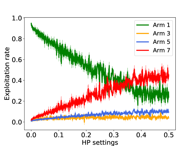
a.1 HP study for $\theta$

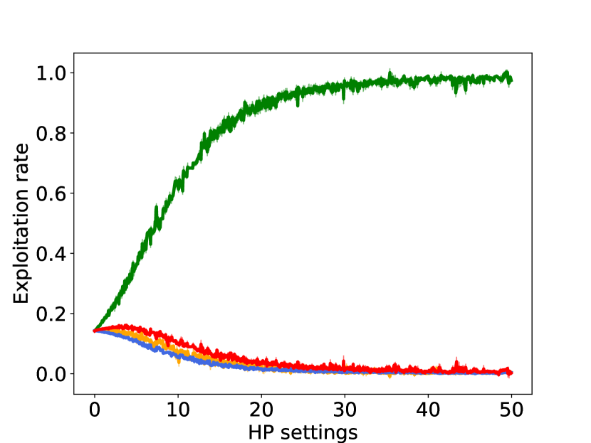
a.2 HP study for $\gamma$

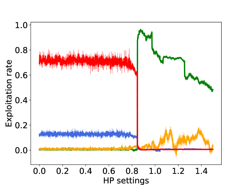
a.3 HP study for $\beta$

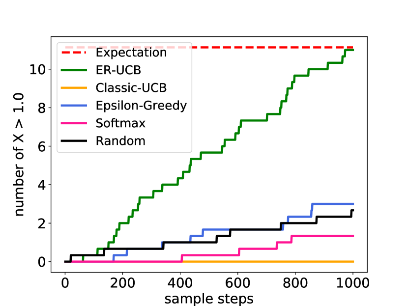
b. Regret study

Figure 1: Illustrations of the results for the synthetic experiment. Figure a.1, a.2, a.3 are the results of the ER-UCB hyper-parameter studies, which illustrate the exploitation rates under the different hyper-parameter settings. The green line of those three figures is the result of arm $1$ which is the best arm. The red line is the result of arm $7$ which has the largest feedback expectation. Figure b shows the results that the number of event $X>1.0$ occurs changes with the number of trials increases. The red dash line is the expectation of the ground-truth strategy. The green line is the proposed ER-UCB strategy.

4 Experiments

In the experiment section, we empirically investigate the effectiveness of the ER-UCB bandit on some synthetic and real-world AutoML tasks. Some state-of-the-art bandit strategies are selected as the compared methods, including the classical UCB (C-UCB) Bubeck et al. (2012), $\epsilon$-greedy Sutton and Barto (2018), softmax strategy Tokic and Palm (2011) and random strategy which allocates the budget by selecting arms randomly. In addition, we apply the random search on the joint hyper-parameter spaces of all algorithms (Joint) to compare with the cascaded hyper-parameter optimization.

4.1 Synthetic problem

We construct a 7-armed bandit problem in this section. The feedbacks obey Gaussian distributions with different expectations and variances: $G_{1}\left(0.84,0.07^{2}\right)$, $G_{2}\left(0.84,0.01^{2}\right)$, $G_{3}\left(0.85,0.04^{2}\right)$, $G_{4}\left(0.85,0.02^{2}\right)$, $G_{5}\left(0.88,0.01^{2}\right)$, $G_{6}\left(0.88,0.02^{2}\right)$, $G_{7}\left(0.89,0.01^{2}\right)\}$. The best arm is not only related with the expectation, but also influenced by the variance. Obviously, it is more likely to obtain the best feedback by exploiting in $G_{1}$, in other words, $i^{*}=1$. We study on the three hyper-parameters of ER-UCB firstly, and then compare the ER-UCB with other methods.

4.1.1 Hyper-parameter study

We investigate the $\theta$, $\gamma$ and $\beta$ for the ER-UCB. With fixed two of them, we study another one: with fixed $\gamma=20$, $\beta=0.85$, we study $\theta\in\left[0.0001,0.5\right]$; with fixed $\beta=0.85$, $\theta=0.01$, we study $\gamma\in\left[0,50\right]$; with fixed $\theta=0.01$, $\gamma=20$, we study $\beta\in\left[0,1.5\right]$. For every hyper-parameter, we evenly sample 1000 settings from the setting region. The core problem we care about is how the methods allocate budget to arms. Let $R^{\text{exi}}_{i}=\frac{T_{i}\left(n\right)}{n}$ define the exploitation rate for arm $i$. Large $R^{\text{exi}}_{i}$ means the large number of trials that the arm $i$ is selected. The trial budget is set as 1000. The experiment for every hyper-parameter setting is repeated for 3 times independently, and the average results are presented.

Figure 1:a.1, 2 and 3 show the study results of $\theta$, $\gamma$ and $\beta$. The arm $1$ is the best selection. Thus, the larger $R^{\text{exi}}_{1}$ the better. For $\theta$ (Figure 1:a.1), the green line ($R^{\text{exi}}_{1}$) is approaching 1 when $\theta$ nears by 0. In practice, $\theta$ should be set as a small value. For $\gamma$ (Figure 1:a.2), when $\gamma$ is small, the exploitation rates of arms are similar. And the green line is increasing during $\gamma$ is increasing. It means that the small $\gamma$ encourages exploration and the large $\gamma$ encourages exploitation according to the observations. For $\beta$ (Figure 1:a.3), the exploitation rates are sensitive to $\beta$ when $\beta$ is around the expectations of reward distributions. Thus, $\beta$ should be carefully tuned according to different tasks.

Table 1: The performance summary of compared bandit strategies on the synthetic problem. $\bar{X}^{*}$ is the average best feedback for three independent runnings. $i_{X^{*}}$ is the arm index that the best feedback is from in each of runnings. $\max_{i}R^{\text{exi}}_{i}$ is the arm index that the strategy allocates the most budget to in each of runnings. The number in bold means the best performance.

Methods	$\bar{X}^{*}$	$i_{X^{*}}$	$\max_{i}R^{\text{exi}}_{i}$	$R^{\text{exi}}_{1}$
ER-UCB	$\bm{1.06}$$\pm$0.02	1,1,1	1,1,1	$\bm{0.90}$$\pm$0.01
C-UCB	0.94$\pm$0.01	1,7,6	7,7,7	0.01$\pm$0.01
$\epsilon$-Greedy	0.98$\pm$0.04	6,1,1	6,1,6	0.31$\pm$0.42
Softmax	1.01$\pm$0.01	1,1,1	7,7,1	0.18$\pm$0.01
Random	1.00$\pm$0.05	1,1,1	4,1,6	0.15$\pm$0.01

4.1.2 Investigation with compared methods

According to the hyper-parameter study results of the ER-UCB, we set $\theta=0.01$, $\gamma=20$, $\beta=0.85$, and compare it with the C-UCB, $\epsilon$-greedy ($\epsilon=0.1$), Softmax strategy ($\tau=0.1$) and random selection strategy. The trial budget is 1000. Every experiment is repeated for 3 times independently. The average performances are presented in Table 1.

Table 1 shows that the ER-UCB outperforms the compared methods. Furthermore, the ER-UCB can find the best arm (arm $1$) and allocate most of budget to it ($\max R^{\text{exi}}_{i}=\{1,1,1\}$ and average $R^{\text{exi}}_{1}$ is 0.9). Because the C-UCB depends only on mean observations to make decisions. It wrongly allocates budget to arm $7$ ($\max R^{\text{exi}}_{i}=\{7,7,7\}$). The $R^{\text{exi}}_{1}$ of $\epsilon$-greedy is very unstable. It means $\epsilon$-greedy can’t find the best arm effectively. In general, the ER-UCB can effectively discover the best-arm and reasonably allocate budget to exploration and exploitation in this synthetic problem.

4.2 Real-word AutoML tasks

We apply the ER-UCB to solve the real-world classification tasks. We select 10 frequently-used algorithms as the candidates from SKLEARN Pedregosa et al. (2011), including DecisionTree (DT), AdaBoost (Ada), QuadraticDiscriminantAnalysis (QDA), GaussianNB (GNB), BernoulliNB (BNB), K-Neighbors (KN), ExtraTree (ET), PassiveAggressive (PA), RandomForest (RF) and SGD. And 12 classification datasets from UCI are selected as AutoML tasks. The evaluation criterion of each configuration is the accuracy score. The compared methods are C-UCB, $\epsilon$-greedy ($\epsilon=0.1$), Softmax strategy ($\tau=0.1$), random strategy and Joint. The trial budget is 1000. We set $\theta=0.01$, $\gamma=20$ for the ER-UCB on all datasets. The $\beta$ is set according to the tasks, and showed in Table 2. For each method and each dataset, we run every experiment 3 times independently, and the average performances of our experiment are presented. In addition, we apply the random search with 1000 trials to explore on every algorithm candidate. According to (2), we can find out the best ground-truth algorithm for the datasets.

Table 2: The average performances on AutoML tasks including the best validation accuracy (V-Eval), the exploitation rate on the ground-truth best algorithm ($R^{\text{exi}}_{i^{*}}$), the best-selected algorithm (B. Alg.) and the test accuracy (T-Eval). The items under the dataset name are the ground-truth algorithm and the $\beta$ setting for the ER-UCB. The number in bold means the best performance in compared methods.

Dataset	Methods	V-Eval	$R^{\text{exi}}_{i^{*}}$	B. Alg.	T-Eval	Dataset	Methods	V-Eval	$R^{\text{exi}}_{i^{*}}$	B. Alg.	T-Eval
Balance (SGD) $\beta=0.5$	ER-UCB	$\bm{.9025}$	$\bm{.5677}$	SGD	$\bm{.9074}$	Car (ET) $\beta=0.6$	ER-UCB	$\bm{.8729}$	$\bm{.9800}$	ET	$\bm{.6937}$
	C-UCB	.8924	.1067	PA	.8339		C-UCB	.8690	.1173	RF	.6416
	$\epsilon$-Greedy	.8931	.0693	SGD	.8227		$\epsilon$-Greedy	.8630	.0277	RF	.6657
	Softmax	.9004	.1287	SGD	.8809		Softmax	.8620	.1163	DT	.6551
	Random	.8978	.1097	SGD	.8597		Random	.8628	.1053	RF	.6839
	Joint	.8978	-	SGD	.8994		Joint	.8619	-	RF	.8604
Chess (Ada) $\beta=0.5$	ER-UCB	$\bm{.9557}$	$\bm{.6137}$	Ada	.8515	Cylinder (ET) $\beta=0.5$	ER-UCB	$\bm{.7356}$	$\bm{.6043}$	ET	$\bm{.6117}$
	C-UCB	.9414	.1693	Ada	$\bm{.8860}$		C-UCB	.7172	.1117	ET	.5534
	$\epsilon$-Greedy	.9492	.3593	Ada	.7510		$\epsilon$-Greedy	.6528	.0443	ET	.5006
	Softmax	.9414	.1290	PA	.8229		Softmax	.6866	.0977	ET	.5749
	Random	.9464	.1070	PA	.6999		Random	.6977	.0990	ET	.5534
	Joint	.9457	-	SGD	.8479		Joint	.6531	-	QDA	.5687
Ecoli (RF) $\beta=0.5$	ER-UCB	$\bm{.8763}$	$\bm{.7013}$	RF	$\bm{.8904}$	Glass (DT) $\beta=0.4$	ER-UCB	$\bm{.7540}$	$\bm{.9716}$	RF	$\bm{.6740}$
	C-UCB	.8745	.2440	RF	.8333		C-UCB	.7265	.1520	RF	.6370
	$\epsilon$-Greedy	.8129	.3023	RF	.8809		$\epsilon$-Greedy	.7163	.0017	RF	.6148
	Softmax	.8728	.1630	RF	.8809		Softmax	.7197	.1180	RF	.6148
	Random	.8695	.1037	RF	.8762		Random	.7247	.1027	RF	.6666
	Joint	.8549	-	RF	.8714		Joint	.7087	-	RF	.6444
Messider (SGD) $\beta=0.5$	ER-UCB	$\bm{.7431}$	$\bm{.5203}$	SGD	.7330	Nursery (Ada) $\beta=0.5$	ER-UCB	$\bm{.8200}$	$\bm{.7640}$	Ada	$\bm{.6909}$
	C-UCB	.7297	.1133	SGD	.7272		C-UCB	.7871	.1370	RF	.6688
	$\epsilon$-Greedy	.7362	.0157	SGD	.7272		$\epsilon$-Greedy	.7201	.0607	Ada	.6457
	Softmax	.7402	.1163	SGD	$\bm{.7604}$		Softmax	.8010	.1150	Ada	.6238
	Random	.7406	.1027	SGD	.7330		Random	.8039	.1100	Ada	.6631
	Joint	.7399	-	SGD	.7316		Joint	.7884	-	Ada	.6304
Spambase (Ada) $\beta=0.7$	ER-UCB	$\bm{.9328}$	$\bm{.9853}$	Ada	.9449	Statlog (Ada) $\beta=0.6$	ER-UCB	$\bm{.9804}$	$\bm{.9763}$	RF	$\bm{.9711}$
	C-UCB	.9298	.1757	Ada	.9457		C-UCB	.9779	.1950	RF	.9696
	$\epsilon$-Greedy	.9311	.7333	Ada	$\bm{.9741}$		$\epsilon$-Greedy	.9790	.8047	RF	.9703
	Softmax	.9298	.1253	Ada	.9471		Softmax	.9768	.1397	RF	.9660
	Random	.9306	.1057	Ada	.9500		Random	.9776	.1203	RF	.9696
	Joint	.9290	-	RF	.9428		Joint	.9793	-	RF	.9464
WDBC (Ada) $\beta=0.6$	ER-UCB	$\bm{.9823}$	$\bm{.9506}$	Ada	.9681	Wilt (Ada) $\beta=0.8$	ER-UCB	$\bm{.9827}$	$\bm{.6206}$	RF	$\bm{.9433}$
	C-UCB	.9808	.1397	Ada	.9710		C-UCB	.9820	.1200	RF	.9320
	$\epsilon$-Greedy	.9816	.8757	Ada	.9681		$\epsilon$-Greedy	.9813	.3567	Ada	.9427
	Softmax	.9794	.1207	Ada	$\bm{.9739}$		Softmax	.9819	.1097	RF	.9267
	Random	.9794	.1060	Ada	$\bm{.9739}$		Random	.9821	.1103	RF	.9347
	Joint	.9794	-	Ada	.9594		Joint	.9821	-	DT	.9320

The average performances of the compared methods on all 12 datasets are presented in Table 2. From Table 2, we can get the following empirical conclusions:

• “No free lunch” has been proved again in those experiments. The best performance algorithms are different in different datasets. Particularly, tree-based ensemble algorithms, e.g., AdaBoost, RandomForest, etc, show the outstanding performance in most of the datasets. It indicates that the algorithm selection is necessary for making search hyper-parameters easier.

• The cascaded algorithm selection and hyper-parameter optimization are necessary for making the search problem easier to solve. Comparing the random strategy with the Joint, the random strategy beats the Joint on most of the datasets (8/12). It indicates that the large search space provides more difficult for optimization.

• It will mislead the strategy to select wrong algorithms only according to the average performance. In Table 2, the random strategy is not always bad in datasets. The strategies, such as C-UCB, $\epsilon$-greedy and Softmax, which focus on the average performance are easy to select wrong algorithms which average performances are good.

• The proposed ER-UCB bandit strategy can effectively find out the best performance algorithm (B. Alg. is the ground-truth algorithm on 9/12 datasets), and reasonably allocate the trial budget to the best algorithm (ER-UCB gets the highest $R^{\text{exi}}_{i^{*}}$ on 12/12 datasets).

5 Conclusion

This paper proposes the extreme-region upper confidence bound (ER-UCB) bandit for the cascaded algorithm selection and hyper-parameter optimization. we employ the random search in the hyper-parameter optimization level. The level of algorithm selection is formulated as a multi-armed bandit problem. The bandit strategies are applied to allocate the limited search budget to the hyper-parameter optimization processes on algorithm candidates. However, the algorithm selection focuses on the algorithm with the maximum performance but not the average performance. To tackle this, we propose the extreme-region UCB (ER-UCB) strategy, which selects the arm with the largest extreme region of the underlying distribution. The theoretical study shows that the ER-UCB has $O\left(K\ln n\right)$ extreme-region regret upper bound, which has the same order with the classical UCB strategy. The experiments on synthetic and real-world AutoML problems empirically verify that the ER-UCB can precisely discover the algorithm with the best performance, and reasonably allocate the trial budget to the algorithm candidates.

References

- Adankon and Cheriet [2009] Mathias M Adankon and Mohamed Cheriet. Model selection for the LS-SVM. application to handwriting recognition. Pattern Recognition, 42(12):3264–3270, 2009.
- Auer et al. [2002] Peter Auer, Nicolo Cesa-Bianchi, and Paul Fischer. Finite-time analysis of the multiarmed bandit problem. Machine Learning, 47(2-3):235–256, 2002.
- Biem [2003] Alain Biem. A model selection criterion for classification: Application to hmm topology optimization. In Proceedings of the 7th International Conference on Document Analysis and Recognition, pages 104–108, 2003.
- Brazdil et al. [2003] Pavel B Brazdil, Carlos Soares, and Joaquim Pinto Da Costa. Ranking learning algorithms: Using IBL and meta-learning on accuracy and time results. Machine Learning, 50(3):251–277, 2003.
- Bubeck et al. [2012] Sébastien Bubeck, Nicolo Cesa-Bianchi, et al. Regret analysis of stochastic and nonstochastic multi-armed bandit problems. Foundations and Trends in Machine Learning, 5(1):1–122, 2012.
- Carpentier and Valko [2014] Alexandra Carpentier and Michal Valko. Extreme bandits. In Advances in Neural Information Processing Systems, pages 1089–1097, 2014.
- Cicirello and Smith [2005] Vincent A Cicirello and Stephen F Smith. The max k-armed bandit: A new model of exploration applied to search heuristic selection. In Proceedings of the 20th AAAI Conference on Artificial Intelligence, pages 1355–1361, 2005.
- Felício et al. [2017] Crícia Z Felício, Klérisson VR Paixão, Celia AZ Barcelos, and Philippe Preux. A multi-armed bandit model selection for cold-start user recommendation. In Proceedings of the 25th Conference on User Modeling, Adaptation and Personalization, pages 32–40. ACM, 2017.
- Feurer et al. [2015] Matthias Feurer, Aaron Klein, Katharina Eggensperger, Jost , Manuel Blum, and Frank Hutter. Efficient and robust automated machine learning. In Advances in Neural Information Processing Systems, pages 2962–2970, 2015.
- Hu et al. [2017] Yi-Qi Hu, Hong Qian, and Yang Yu. Sequential classification-based optimization for direct policy search. In Proceedings of the 31st AAAI Conference on Artificial Intelligence, pages 2029–2035, 2017.
- Hu et al. [2018] Yi-Qi Hu, Yang Yu, and Zhi-Hua Zhou. Experienced optimization with reusable directional model for hyper-parameter search. In Proceeding of the 27th International Joint Conference on Artificial Intelligence, pages 2276–2282, 2018.
- Hu et al. [2019] Yi-Qi Hu, Yang Yu, Wei-Wei Tu, Qiang Yang, Yuqiang Chen, and Wenyuan Dai. Multi-fidelity automatic hyper-parameter tuning via transfer series expansion. In Proceedings of the 33rd AAAI Conference on Artificial Intelligence, 2019.
- Hutter et al. [2011] Frank Hutter, Holger H Hoos, and Kevin Leyton-Brown. Sequential model-based optimization for general algorithm configuration. LION, 5:507–523, 2011.
- Jamieson and Talwalkar [2016] Kevin G Jamieson and Ameet Talwalkar. Non-stochastic best arm identification and hyperparameter optimization. In Proceedings of the 19th International Conference on Artificial Intelligence and Statistics, pages 240–248, 2016.
- Pedregosa et al. [2011] Fabian Pedregosa, Gael Varoquaux, Alexandre Gramfort, Vincent Michel, Bertrand Thirion, Olivier Grisel, Mathieu Blondel, Peter Prettenhofer, Ron Weiss, Vincent Dubourg, Jake Vanderplas, Alexandre Passos, David Cournapeau, Matthieu Brucher, Matthieu Perrot, and Edouard Duchesnay. Scikit-learn: Machine learning in Python. Journal of Machine Learning Research, 12:2825–2830, 2011.
- Sutton and Barto [2018] Richard S Sutton and Andrew G Barto. Reinforcement learning: An introduction. MIT press, 2018.
- Thornton et al. [2013] Chris Thornton, Frank Hutter, Holger H Hoos, and Kevin Leyton-Brown. Auto-weka: Combined selection and hyperparameter optimization of classification algorithms. In Proceedings of the 19th ACM SIGKDD International Conference on Knowledge Discovery and Data Mining, pages 847–855, 2013.
- Tokic and Palm [2011] Michel Tokic and Günther Palm. Value-difference based exploration: adaptive control between epsilon-greedy and softmax. In Annual Conference on Artificial Intelligence, pages 335–346. Springer, 2011.
- Yu et al. [2016] Yang Yu, Hong Qian, and Yi-Qi Hu. Derivative-free optimization via classification. In Proceedings of the 30th AAAI Conference on Artificial Intelligence, pages 2286–2292, 2016.