Periodic projections of alternating knots

Abstract

This paper is devoted to prove the existence of $q$-periodic alternating projections of prime alternating $q$-periodic knots. The main tool is the Menasco-Thistlethwaite’s Flyping theorem.

Let $K$ be an oriented prime alternating knot that is $q$-periodic with $q\geq 3$, i.e. $K$ admits a symmetry that is a rotation of order $q$. Then $K$ has an alternating $q$-periodic projection.
As applications, we obtain the crossing number of a $q$-periodic alternating knot with $q\geq 3$ is a multiple of $q$ and we give an elementary proof that the knot $12_{a634}$ is not 3-periodic; this proof does not depend on computer computations as in [11].

1 Introduction

In this paper, links (knots are one-component links) in $S^{3}$ and projections in $S^{2}$ are assumed, unless otherwise indicated, prime and oriented.
The purpose of this paper is the study of the visibility of the periodicity of alternating knots on alternating projections initiated in [5]. The main result is:

Visibility Theorem 3.1 Let $K$ be an oriented prime alternating knot that is $q$-periodic with $q\geq 3$. Then $K$ has a $q$-periodic alternating projection.

We also obtain the following applications:

1. If Seifert’s algorithm is applied on a $q$-periodic projection of an oriented link, the resulting surface exhibits a $q$-periodic symmetry. Such a surface is called $q$-equivariant. The topological types of periodic homeomorphisms of bordered surfaces that are equivariant Seifert surfaces of periodic links are studied in [4]. A. Edmonds [6] shows that if a knot $K$ is of period $q$, then there is a $q$-equivariant Seifert surface for $K$, which has the genus of $K$. For $K$ a $q$-periodic prime oriented alternating knot with $q\geq 3$, the strategy explained in the proof of Theorem 3.1 enables to exhibit the realization of a $q$-equivariant surface from Seifert’s algorithm which has the genus of $K$.

2. The following result is also a direct consequence of Theorem 3.1:

Proposition 3.4 (Conjecture in Section 1.4 of [5]) The crossing number of a $q$-periodic alternating knot with $q\geq 3$ is a multiple of $q$.

3. The Murasugi decomposition into atoms of $12a_{634}$ gives rise to an adjacency graph which is a tree of 2-vertices ([16], [17]). According to Visibility Theorem 3.1 and Lemma 3.2 (which is an application of Corollary 1 in [5]), we deduce that $12a_{634}$ is not 3-periodic. We thank C. Livingstone to point out the existence of a computer proof of this fact by S. Jabuka and S. Naik [11].

1.1 Organization of the paper

For the study of the visibility of the periodicity of the alternating knots on alternating projections, we will call upon the canonical decomposition of link projections recalled in §2, as it was done for the visibility of achirality of the alternating knots in [8]. The decomposition of a link projection $\Pi$ is carried out by a family of canonical Conway circles which decomposes $(S^{2},\Pi)$ into diagrams called jewels and twisted band diagrams; the arborescent part of $\Pi$ is the union of the twisted band diagrams of $\Pi$. The decomposition of the diagram $(S^{2},\Pi)$ by the canonical Conway circles is a 2-dimensional version of the decomposition of Bonahon-Siebenman [1] of $(S^{3},K)$ into an algebraic part $(A,A\cap K)$ and a non-algebraic part $(N,N\cap K)$. Each component of $\partial A=\partial N$ is a 2-sphere that cuts $K$ in four points and is called a Conway sphere. We now assume that links and projections we consider are alternating. In our terminology, the 2-dimensional notion “arborescent” implies the 3-dimensional notion “algebraic” (see the definition for instance in [18]). The projection of a Conway sphere on $S^{2}$ is a Conway circle. The inverse is not true: there are “hidden” Conway spheres that do not project on Conway circles on alternating projections ([18]). However since our point of view is strictly 2-dimensional and based only on alternating projections, this case does not affect us.
The notion of flype in alternating projections (Fig. 7) is at the heart of our analysis and lies completely in their arborescent part. According to Menasco-Thistlethwaite’s Flyping theorem [14], two reduced alternating projections $\Pi_{1}$ and $\Pi_{2}$ of an isotopy class of an alternating link $K$ are related by a finite sequence of flypes, up to homeomorphisms of $S^{2}$ onto itself. Starting from the canonical decomposition of a projection of $\Pi(K)$ of $K$, we associate canonical and essential structure trees (as recalled in §2) that does not depend on the choice of an alternating projection. The canonical and essential structure trees are invariants of the isotopy class of alternating knots. For example, for rational links, their canonical structure tree is a linear tree with integer-weighted vertices and their essential structure tree is reduced to a vertex of rational weight.

In §3 we study how the $q$-periodicity acts on the essential Conway circles and on the diagrams of any alternating projection. With the help of Kerekjarto’s theorem [3] and Flyping Theorem of Menasco-Thistlethwaite we prove Theorem 3.1 and we obtain a $q$-periodic alternating projection by adjustments with flypes on any alternating prime $q$-periodic knot. With the help of the Murasugi decomposition into atoms for periodic alternating knots and a result in [5] which links the $q$-periodicity of an alternating knot to the $q$-periodicity of its atoms, we finally show that $12a_{634}$ is not 3-periodic.

2 Canonical Decomposition of a Projection

In this section we do not assume that link projections are alternating. A projection on $S^{2}$ is the image of a link in $S^{3}$ by a generic projection onto $S^{2}$, hence a labeled graph with $n$ 4-valent crossing-vertices labeled to reflect under and over crossings.
In this paper the term “ diagram” will be used to refer to a different object (see below §2.1).

2.1 Diagrams

Let $\Sigma$ be a compact connected planar surface embedded on the projection sphere $S^{2}$. We denote by $k+1$ the number of connected components of its boundary $\partial\Sigma$.

Definition 2.1.

The pair $D=(\Sigma,\Gamma=\Pi\cap\Sigma)$ where $\Pi$ is a link projection is called a diagram if for each connected component $C$ of $\partial\Sigma$, $C\cap\Pi$ is composed exactly of 4 points.

Remark 2.1.

A (link) projection $\Pi$ on $S^{2}$ is a diagram $(\Sigma,\Pi)$ where $\Sigma=S^{2}$.

Definition 2.2.

(1) A trivial diagram is a diagram homeomorphic to $\mathrm{T([\infty])}$ (Fig. $1(a)$).
(2) A singleton is a diagram homeomorphic to Fig. 1(b).

Figure 1: $(a)$ Tangle $\mathrm{T([\infty])}$   $(b)$ A singleton

Definition 2.3.

A Haseman circle of a diagram $D=(\Sigma,\Gamma)$ is a circle $\gamma\subset\Sigma$ that intersects the projection $\Pi$ exactly in 4 points away from crossing points. A Haseman circle is said to be compressible if $\gamma$ bounds a disc $\Delta$ in $\Sigma$ such that $(\Delta,\Gamma\cap\Delta)$ is either a trivial diagram or a singleton.

In what follows, Haseman circles are not compressible. We therefore only consider diagrams that are neither trivial diagrams nor singletons.

Definition 2.4.

A twisted band diagram (TBD) is a diagram homeomorphic to Fig. 3.

The signed weight of a crossing on a band is defined according to Fig. 2. It depends on the direction of the half-twist of the band supporting the crossing.

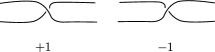
Figure 2: The signed weight of a crossing on a band

Figure 3: A twisted band diagram

In Fig. 3 the boundary components of $\Sigma$ are denoted $\gamma_{1},\dots,\gamma_{k+1}$ where $k\geq 0$. The corresponding portion of the band diagram between the projection and the circles $\gamma_{i}$ and $\gamma_{i+1}$ is called a twist region with $|a_{i}|$ crossing points. The sign of $a_{i}$ is the signed weight of the $|a_{i}|$ crossing points. The integer $a_{i}$ will be called an intermediate weight.
If $k+1=1$, the planar surface $\Sigma$ is a disc and the twisted band diagram $(\Sigma,\Sigma\cap\Pi)$ is called a spire with $|a_{1}|\geq 2$ crossings.
If $k+1=2$, the twisted band diagram is a twisted annulus and we require that $a_{1}+a_{2}\neq 0$.

We ask the crossings on the same band to have the same signed weight. In other words, using flypes (Fig. 7) and Reidemeister move 2, we can reduce the number of crossing points of a twisted band diagram so that all non zero intermediate weights $a_{i}$ of a twisted band diagram have the same sign.

Definition 2.5.

(1) The crossings of a TBD (twisted band diagram) $(\Sigma,\Sigma\cap\Pi)$ are called the visible crossings of $(\Sigma,\Sigma\cap\Pi)$.
(2) The sum $a=\Sigma a_{i}$ is called the total weight of the twisted band diagram $(\Sigma,\Sigma\cap\Pi)$. If $k+1\geq 3$ we may have $a=0$. The absolute value of $a$ is equal to the number of the visible crossings of $(\Sigma,\Sigma\cap\Pi)$.

Two Haseman circles are said to be parallel if they bound an annulus $A\subset\Sigma$ such that the pair $(A,A\cap\Gamma)$ is diffeomorphic to Fig. 4.

Figure 4: Parallel Haseman circles

We define a Haseman circle $\gamma$ to be boundary parallel if there exists an annulus $A\subset\Sigma$ such that:
(1) the boundary $\partial A$ of $A$ is the disjoint union of $\gamma$ and a boundary component of $\Sigma$;
(2) $(A,A\cap\Gamma)$ is diffeomorphic to Fig. 4.

Definition 2.6.

A jewel is a diagram $J$ such that:
(1) it is not a twisted band diagram with $k+1=2$ and $a=\pm 1$ or with $k+1=3$ and $a=0$.
(2) each Haseman circle of $J$ is boundary parallel.

Fig. 5 depicts a jewel $\mathrm{J=(\Sigma,\Pi\cap\Sigma)}$ where $\Sigma$ is a planar surface with boundary $\partial\Sigma=\gamma_{1}\cup\gamma_{2}\cup\gamma_{3}\cup\gamma_{4}$.

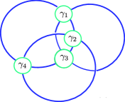
Figure 5: A jewel

2.2 Families of Haseman circles for a projection

2.2.1 Canonical Conway circles

If not otherwise stated, the projections we consider are connected and prime.

Definition 2.7.

Let $\Pi$ be a projection. A family of Haseman circles for $\Pi$ is a set of Haseman circles satisfying the following conditions:
(1) any two circles are disjoint and
(2) no two circles are parallel.

Let $\mathcal{H}=\{\gamma_{1},...,\gamma_{n}\}$ be a family of Haseman circles for $\Pi$. Let $R$ be the closure of a connected component of $S^{2}\setminus\bigcup_{i=1}^{i=n}\gamma_{i}$. We call the pair $(R,R\cap\Pi)$ a diagram of $\Pi$ determined by the family $\mathcal{H}$.

Definition 2.8.

A family $\mathcal{C}$ of Haseman circles is an admissible family if each diagram determined by it is either a twisted band diagram or a jewel. An admissible family is minimal if removing a circle turns it into a family that is not admissible.

Theorem 2.1 is the main structure theorem about link projections proved in ([15], Theorem 1). It is essentially due to Bonahon and Siebenmann.

Figure 6: A non canonical Conway circle

Theorem 2.1.

(Existence and uniqueness theorem of minimal admissible families) Let $\Pi$ be a link projection in $S^{2}$. Then:
i) there exist minimal admissible families for $\Pi$;
ii) any two minimal admissible families are isotopic by an isotopy respecting $\Pi$.

Definition 2.9.

An Haseman circle belonging to “the” minimal admissible family of $\Pi$ noted $\mathcal{C}_{can}$ is called a canonical Conway circle of the projection $\Pi$.

Example 1.

The Haseman circle $C$ in Fig. 6 is not a canonical Conway circle.

The decomposition of $\Pi$ into twisted band diagrams and jewels determined by $\mathcal{C}_{can}$ will be called the canonical decomposition of $\Pi$. If there are no jewels in its canonical decomposition, the projection $\Pi$ is said to be arborescent.

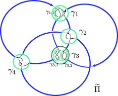
Figure 7: A projection with its canonical Conway circles

A canonical Conway circle can be of 3 types:
(1) a circle that separates two jewels.
(2) a circle that separates two twisted band diagrams.
(3) a circle that separates a jewel and a twisted band diagram.

Example 2.

Fig. 7 illustrates a projection $\widetilde{\Pi}$ with its canonical Conway family:

$$\mathcal{C}_{can}(\widetilde{\Pi})=\{\gamma_{1},\gamma_{1,1},\gamma_{2},\gamma_{3},\gamma_{3,1},\gamma_{3,2},\gamma_{4}\}.$$

Figure 8: $10^{***}$ is a tangle sum of two $6^{*}$

Remark 2.2.

1. As remarked in [8], our notion of jewel is more restrictive than the notion of John Conway polyhedron ([13] p. 139). We define a jewel graph $G_{J}$ of a jewel $J$ by collapsing each Haseman circle of $J$ to a vertex. For John Conway, the graph of a basic polyhedron is a simple regular graph of valency 4. A basic polyhedron can therefore be a tangle sum of several jewel graphs. A jewel graph is simply a polyhedron in the sense of John Conway, indecomposable with regard to the tangle sum. The polyhedron $10^{\ast\ast\ast}$ has a non-trivial Haseman circle (see Fig. 8).

2. The minimal projection of the torus link of type $(2,m)$ can be considered as a twisted band diagram with $k+1=0$.

2.2.2 Essential Conway circles

Let $\Pi$ be a projection on $S^{2}$.

Definition 2.10.

A (2-dimensional) tangle $\mathcal{T}$ of $\Pi$ is a pair $\mathcal{T}=(\Delta,\tau_{\Delta})$ where $\Delta$ is a disk in $S^{2}$, $\tau_{\Delta}$ is $\Pi\cap\Delta$ and the boundary $\partial\Delta$ of $\Delta$ intersects $\tau_{\Delta}$ exactly on 4 points.
The boundary $\partial\mathcal{T}$ of $\mathcal{T}$ is the boundary $\partial\Delta$ of $\Delta$.

Note that a (2-dimensional) tangle is the projection onto the equatorial disk of the 3-ball of a (3-dimensional) tangle which will be defined further in Definition 3.4.

Definition 2.11.

Two tangles $\mathcal{T}=(\Delta,\tau_{\Delta})$ and $\mathcal{T}{{}^{\prime}}=(\Delta,\tau_{\Delta}^{\prime})$ are isotopic if there exists a homeomorphism $f:\mathcal{T}\rightarrow\mathcal{T}{{}^{\prime}}$ such that:
(1) $f$ is the identity on the boundary $\partial\Delta$ and
(2) $f(\tau_{\Delta})=\tau_{\Delta}^{\prime}$.

Definition 2.12.

A rational tangle is a tangle such that all its canonical Conway circles are concentric and delimit twisted annuli, with the exception of the innermost circle which is the boundary of a spire, as shown in Fig. 9.
A maximal rational tangle of a link projection $\Pi$ is a rational tangle that is not strictly included in a larger rational tangle of $\Pi$.

Let $\mathcal{T}$ be a rational tangle. We now consider $\mathcal{T}$ under the cardan form $\mathrm{T}[a_{0},\dots,a_{m}]$ (or equivalently under the standard form described in [12]) illustrated in Fig. 9 such that the twisted band diagrams have weights $b_{i}=(-1)^{i}a_{i}$ with $i=0,\dots,m$ and such that the first weight band $b_{0}$ is horizontal.

To $\mathrm{T}[a_{0},\dots,a_{m}]$ where $a_{0}\in\mathbb{Z}$ and $a_{1},\dots,a_{m}\in\mathbb{Z}-\{0\}$, we assign the continued fraction

$$[a_{0},a_{2},\cdots a_{m}]=a_{0}+\dfrac{1}{a_{1}+\dfrac{1}{{\ddots}+\dfrac{1}{a_{m}}}}$$

If $\mathcal{T}$ is not the trivial tangle $\mathrm{T([\infty])}$ (Fig. $1(a)$), the rational number ${\frac{r}{s}}=[a_{0},a_{2},\cdots a_{m}]$ with $(r,s)=1$ and $r>0$ is called the fraction $\mathrm{F(}\mathcal{T}\mathrm{)}$.
By convention, the fraction of the trivial tangle $\mathrm{T([\infty])}$ is: $\mathrm{F(T([\infty]):=\infty}$.

The fraction is an isotopy invariant of the tangle $\mathcal{T}$. It means that with the expansion of $\frac{r}{s}$ in another continuous fraction $[d_{0},\dots,d_{k}]$, we get another cardan tangle $\mathrm{T}[d_{0},\dots,d_{k}]$ isotopic to $\mathrm{T}[a_{0},\dots,a_{m}]$. We will use $\mathrm{T}_{\frac{r}{s}}$ to denote a rational tangle with fraction $\frac{r}{s}$.

Figure 9: $\mathrm{T}[a_{0},\dots,a_{m}]$

Remark 2.3.

Let ${\frac{r}{s}}$ be a rational number with $r>0$ and $(r,s)=1$. Then ${\frac{r}{s}}$ has an expansion $[a_{0},\dots,a_{m}]$ where the $a_{i}$’s are all positive or all negative; it is called a homogeneous continued fraction. If furthermore, $a_{0}$ and $a_{m}$ are not equal to $\pm 1$, the continued fraction $[a_{0},\dots,a_{m}]$ is said to be strictly homogeneous. If $[a_{0},\dots,a_{m}]$ is a homogeneous continued fraction, the cardan tangle $\mathrm{T}[a_{0},\dots,a_{m}]$ is an alternating tangle.

Definition 2.13.

An essential Conway circle of an alternating projection $\Pi$ is a canonical Conway circle that is not properly contained in a maximal rational tangle.

In a rational link projection, there are no essential Conway circles.

Let $\Pi$ be a non-rational link projection. By removing from the minimal admissible family $\mathcal{C}_{can}$ of $\Pi$ all concentric Conway circles of each maximal rational tangle $\mathcal{T}$ of $(S^{2},\Pi)$ except its boundary circle $\partial\mathcal{T}$, we obtain the essential Conway family of $\Pi$ denoted $\mathcal{C}_{ess}(\Pi)$.

Remark 2.4.

The set of essential Conway circles is empty for an alternating projection if only if the projection is one of the three following cases:
a) a standard torus knot projection of type $(2,s)$ (in this case it can be considered as a twisted band diagram with empty boundary (Remark 2.2.2)),
b) a jewel without boundary
c) a minimal projection of a rational knot.

Figure 10: The essential Conway family of the projection $\widetilde{\Pi}$ illustrated in Fig. 7

Figure 11: A projection with its set $\mathcal{C}_{ess}=\{\mathcal{C}$, $\mathcal{C^{\prime}}$, $\mathcal{C^{\prime\prime}\}}$

Example 3.

1) Fig. 10 illustrates the essential Conway family $\mathcal{C}_{ess}(\widetilde{\Pi})$ of the projection $\widetilde{\Pi}$ of Fig. 7:

$$\mathcal{C}_{ess}(\widetilde{\Pi})=\{\gamma_{1},\gamma_{2},\gamma_{3},\gamma_{3,1},\gamma_{3,2},\gamma_{4}\}.$$

2) In the projection depicted in Fig. 11, $\mathcal{C^{\prime}}$, $\mathcal{C^{\prime\prime}}$ and $\mathcal{C}=\partial\mathrm{T}[a_{0},\dots,a_{m}]$ are essential Conway circles while dotted circles are just canonical Conway circles.

2.3 Canonical and Essential Structure Trees

We now focus the canonical decomposition of alternating link projections.

2.3.1 Flypes and Flyping Theorem

Let $\Pi$ be a $n$-crossing regular projection of a link $L\hookrightarrow S^{3}$ on the projection plane $S^{2}$. As in [14], consider $n$ disjoint small “crossing ball” neighbourhoods $B_{1},\dots,B_{n}$ of the crossing points $c_{1},\dots c_{n}$ of $\Pi$. Then assume that $L$ coincides with $\Pi$, except that inside each $B_{i}$ the two arcs forming $\alpha(c_{i})=\Pi\cap B_{i}$ are perturbed vertically to form semicircular overcrossing and undercrossing arcs, which lie on the boundary of $B_{i}$. This relationship between the link $L$ and its projection $\Pi$ is expressed as $L=\lambda(\Pi)$ ([14]). Note that there is a homeomorphism of pairs $(S^{3},L)\rightarrow(S^{3},\lambda(\Pi))$. We call $\lambda(\Pi)$ a realized projection (or a realized diagram in the terms of [2]) for $L$.

We can consider the ambient space $S^{3}$ to be ${\mathbb{R}^{3}}\cup\{\infty\}$, and we shall take the 2-sphere $S^{2}$ on which the regular projection $\Pi$ lies to be $S^{2}=\{\mathbf{x}\in\mathbb{R}^{3}:\left\|\mathbf{x}\right\|=1\}$. We assume that the knot $\lambda(\Pi)$ lies within the neighborhood $N=\{x\in\mathbb{R}^{3}:{\frac{1}{2}}\leq\left\|{\mathbf{x}}\right\|\leq{\frac{3}{2}}\}$.

Definition 2.14.

Let $g:(S^{3},\lambda(\Pi_{1}))\rightarrow(S^{3},\lambda(\Pi_{2}))$ be a homeomorphism of pairs. The homeomorphism of pairs $g$ is flat if $g$ is pairwise isotopic to a homeomorphism of pairs $h$ with the condition that $h$ maps $N$ onto itself and $h|_{N}=h_{0}\times id_{[{\frac{1}{2}},{\frac{3}{2}}]}$ for some orientation-preserving homeomorphism $h_{0}:S^{2}\rightarrow S^{2}$. We call $h_{0}$ the principal part of the flat homeomorphism $g$.

By asking the crossing balls to be sent on the crossing balls, a flat homeomorphism of pairs is an isomorphism of realized projections as defined in [2].

Definition 2.15.

An isomorphism of realized projections $h:\lambda(\Pi)\rightarrow\lambda(\Pi_{\ast})$ is a homeomorphism of pairs $h:(S^{3},L)\rightarrow(\tilde{S}^{3},\widetilde{L})$ such that:
(1) $h(S^{2})={S}^{2}$,
(2) $h(B_{i})=\widetilde{B}_{i}$ and
(3) $h(\alpha(c_{i}))=\alpha(\tilde{c}_{i})$.

We recall the definition of a flype as described in [14].

Definition 2.16.

Let $\Pi_{1}$ be a projection with the pattern described in Fig. 12(a). A standard flype of $(S^{3},\lambda(\Pi_{1}))$ is any homeomorphism $f$ which maps $(S^{3},\lambda(\Pi_{1}))$ to a pair $(S^{3},\lambda(\Pi_{2}))$ where $\Pi_{2}$ is the pattern described in Fig. 12(b), in such a way that:
(1) $f$ sends the 3-ball $B_{\mathrm{A}}$ into itself by a rigid rotation about an axis in the projection plane,
(2) $f$ fixes pointwise the 3-ball $B_{\mathrm{B}}$,
(3) $f$ moves the crossing visible on the left of Fig. 12(a) to the crossing visible on the right of Fig. 12(b).

Definition 2.17.

Let $\Pi_{1}$ be any projection. Then a flype is any homeomorphism $f:(S^{3},\lambda(\Pi_{1}))\rightarrow(S^{3},\lambda(\Pi_{1}))$ of the form $f=g_{1}\circ f^{\prime}\circ g_{2}$ where $f^{\prime}$ is a standard flype and $g_{1}$ and $g_{2}$ are flat homeomorphisms.

If the tangle $A$ of Fig. 12 contains no crossing, then the standard flype determined by that figure is a flat homeomorphism; therefore according to the above definition, any flat homeomorphism is a flype. We call it a trivial flype.

A 2-dimensional description of a standard flype, as in Fig. 12, is sufficient since it corresponds to a unique standard flype up to isomorphism of realized diagrams. The crossing that moves during the (2-dimensional) flype is an active crossing point of the flype.

Terminology. If there is no possible confusion, we will also designate the (2-dimensional) flype by flype.

Figure 12: A flype

We can now precisely locate where flypes can be performed with respect to the canonical Conway decomposition of a prime alternating reduced link.

Theorem 2.2.

[15] (Position of flypes) Let $\Pi$ be a prime alternating reduced link projection in $S^{2}$ and suppose that a flype can be done in $\Pi$. Then, its active crossing point belongs to a diagram determined by $\mathcal{C}_{can}(\Pi)$. The flype moves the active crossing point either within the twist region to which it belongs or to another twist region of the same twisted band diagram.

Figure 13: An efficient flype

Remark 2.5.

(1) We are only interested in efficient flypes that move the active crossing point from one twist region to another in the same twist band diagram.

(2) Let $\mathcal{T}$ be a TBD of $\Pi$ and $C_{1},C_{2},\dots,C_{k},C_{1}$ be its cyclic sequence of $\mathcal{C}_{can}|_{\mathcal{T}}$. A flype on $\mathcal{T}$ does not modify the order of occurence of the Conway circles $\mathcal{C}_{can}|_{\mathcal{T}}$ in the cyclic sequence.

Definition 2.18.

(1) The set of the twist regions of a given twisted band diagram is called a flype orbit (Fig. 14).
(2) The cardinal of $\mathcal{C}_{can}|_{\mathcal{T}}$ is the valency $k+1$ of the TBD $\mathcal{T}$.

Figure 14: A flype orbit

Corollary 2.1.

[15]
(1) A flype moves an active crossing point inside the flype orbit to which it belongs.
(2) Two distinct flype orbits are disjoint.

This implies that an active crossing point belongs to one and only one TBD. Since two TBD have at most one canonical Conway circle, Corollary 2.1 can be interpreted as a loose kind of commutativity of flypes.

2.3.2 Canonical Structure Tree ${\mathcal{A}}(L)$.

Fundamental to our purposes is the following Menasco-Thistlethwaite Flyping Theorem [14]:

Let $\Pi_{1}$ and $\Pi_{2}$ be two reduced, prime, oriented, alternating projections of links. If $f:(S^{3},\lambda(\Pi_{1}))\rightarrow(S^{3},\lambda(\Pi_{2}))$ is a homeomorphism of pairs, then $f$ is a composition of flypes and flat homeomorphisms.

Since two realizations of alternating projections in $S^{2}$ of the same isotopy class of an oriented prime alternating link in $S^{3}$ are related by flypes, their canonical and essential structure trees constructed as described below, are isomorphic.

Construction of the canonical structure tree ${\mathcal{A}}(L)$.

Let $L$ be a prime alternating link and let $\Pi$ be an alternating projection of $L$. Let $\mathcal{C}_{can}$ be the canonical Conway family for $\Pi$. We construct the canonical structure tree ${\mathcal{A}}(L)$ as follows: its vertices are in bijection with the diagrams determined by $\mathcal{C}_{can}$ and its edges are in bijection with the canonical circles; the vertices of each edge represent the diagrams which both have in their boundary, the canonical circle $\gamma$ corresponding to the edge. Since $S^{2}$ has genus zero, the constructed graph is a tree.
We label the vertices of ${\mathcal{A}}(L)$ as follows: if a vertex represents a twisted band diagram, we label it by its total weight $a$ and if it represents a jewel, we label it with the letter $J$.

In the case of a tangle $\mathcal{T}$ whose boundary is a canonical Conway circle $\gamma$, the canonical structure tree ${\mathcal{A}}(\mathcal{T})$ of $\mathcal{T}$ is a graph such that all its edges have two vertices at the extremities except for an“open” edge (with a single vertex) which represents the circle $\gamma$. For an example, see Fig. 16.

Proposition 2.1.

The canonical structure tree ${\mathcal{A}}(L)$ is independent of the alternating projection chosen to represent $L$.

Proof.

Let $\Pi$ be an alternating link projection in $S^{2}$. By [15], Theorem 1:
i) there exist minimal Conway families for $\Pi$ and
ii) any two minimal Conway families are isotopic, by an isotopy which respects $\Pi$.

A flype or a flat homeomorphism does not modify the canonical structure tree. By Flyping Theorem, we conclude that the canonical structure tree is independent of the chosen alternating projection $\Pi$ and we can speak of the canonical structure tree of $L$ (and not only of $\Pi$). ∎

Definition 2.19.

The alternating knot $K$ is arborescent if each vertex of ${\mathcal{A}}(K)$ has an integer weight.

Example 4.

The link $K_{0}$ which has the projection $\widetilde{\Pi}$ represented by Fig. 7, has its canonical structure tree ${\mathcal{A}}(K_{0})$ given by Fig. $15(a)$.

Figure 15: Canonical structure tree and essential structure tree of $K_{0}$

Remark 2.6.

If the projection $\Pi$ is arborescent, we can encode $\Pi$ with a weighted planar tree à la Bonahon-Siebenman (§5 in [15]) which is a canonical structure tree with more complete information.

2.3.3 Essential Structure Tree $\mathcal{\tilde{A}}(L)$.

Construction of the essential structure tree $\mathcal{\tilde{A}}(L)$.

On the same lines of the construction of the canonical structure tree ${\mathcal{A}}(L)$, we construct the essential structure tree $\widetilde{\mathcal{A}}(L)$. The vertices of $\widetilde{\mathcal{A}}$ are in bijection with the diagrams determined by the set $\mathcal{C}_{ess}(\Pi)$ and the edges are in bijection with the circles of $\mathcal{C}_{ess}(\Pi)$. The extremities of an edge corresponding to an essential Conway circle $\gamma$ are two vertices associated to the two diagrams having $\gamma$ in their boundary.

As in the case with the canonical structure tree, Flyping Theorem implies that:

Proposition 2.2.

The essential structure tree ${\mathcal{\widetilde{A}}}(L)$ is independent of the minimal projection chosen to represent $K$.

The essential structure tree of a tangle: To a tangle $\mathcal{T}$ with an essential Conway circle $\gamma$ as boundary, we associate an essential structure tree denoted $\widetilde{\mathcal{A}}(\mathcal{T})$ which has only one “open edge” with one vertex-end. The unique edge of $\widetilde{\mathcal{A}}(\mathcal{T})$ corresponds to $\gamma$.

Remark 2.7.

1. If $\mathrm{T}_{\frac{p}{q}}$ is a maximal rational tangle, $\widetilde{\mathcal{A}}({\mathrm{T}_{\frac{p}{q}}})$ is a linear graph composed only with an “open” edge and one vertex labelled by ${\frac{p}{q}}$.

2. A vertex in ${\mathcal{\widetilde{A}}}(K)$ with weight $\in\mathbb{Q}\setminus\mathbb{Z}$ is monovalent and its union with its single edge corresponds to a maximal rational tangle in $\Pi$.

3. Only monovalent vertices of an essential structure tree of a link can have weights that are $\in\mathbb{Q}\setminus\mathbb{Z}$

The essential structure tree ${\mathcal{\widetilde{A}}}(\mathrm{T}_{\frac{r}{s}})$ is reduced to a vertex of weight $\frac{r}{s}$.

Figure 16: $(a)$ Canonical structure tree of $\mathcal{A}(\mathrm{T}[-1,-2])$ and $(b)$ Essential structure tree of $\widetilde{\mathcal{A}}(\mathrm{T}[-1,-2])$

Example 5.

$\mathcal{A}(\mathrm{T}[-1,-2])$ and $\widetilde{\mathcal{A}}(\mathrm{T}[-1,-2])$ are described in Fig. 16.

Remark 2.8.

The essential structure tree ${\mathcal{\widetilde{A}}}(K)$ is reduced to a single vertex if and only if $K$ is a rational link $\mathrm{T}_{\frac{r}{s}}$ or is a link described by a jewel without boundary.

3 On Visibility Theorem 3.1

This section is about the proof of the Visibility Theorem 3.1 for $q$-periodic alternating prime knots:

Theorem 3.1.

Let $K$ be an oriented prime alternating knot that is $q$-periodic with $q\geq 3$. Then there exists a $q$-periodic alternating projection $\widetilde{\Pi}$ for $K$.

We first recall the definition of a $q$-periodic knot in $S^{3}$.

Definition 3.1.

A knot $K$ is $q$-periodic if there is a (auto)-homeomorphism $\Phi$ of pairs $(S^{3},K)$ of period $q$ which satisfies the following conditions:
(1) $\Phi$ is a $\frac{2\pi}{q}$-rotation about a “line” (circle) $\alpha$ in $S^{3}$ and
(2) $\alpha\cap K=\varnothing$.
$\Phi$ is called a $q$-homeomorphism of $(S^{3},K)$.

Remark 3.1.

Let $K$ be a $q$-periodic knot with $\Phi$ a $q$-homeomorphism of $(S^{3},K)$. For each divisor $p$ of $q$, $K$ is $p$-periodic with its $p$-homeomorphism $\Psi_{r}=\Phi^{r}$ where $r={\frac{q}{p}}$.

For our ends, we introduce the following notion:

Definition 3.2.

1) If a knot $K$ is $q$-periodic but not strictly $q$-periodic then $K$ is $rq$-periodic for some $r\geq 2$.
2) If a projection $\Pi$ is $q$-periodic but not strictly $q$-periodic then $\Pi$ is $rq$-periodic for some $r\geq 2$.

Figure 17: A non-strictly 4-periodic projection

Example 6.

Let $\Pi$ be an alternating projection described in Fig.17 where $\mathrm{Y}$ is an alternating tangle with boundary an essential Conway circle. The big red circles do not belong to $\mathcal{C}_{ess}(\Pi)$ and hence do not appear on $\mathcal{\ }\tilde{A}(K)$. The projection $\Pi$ is not strictly 4-periodic since as shown by Fig. 17, $\Pi$ is an 8-periodic projection.
Note that the projection $\Pi$ depicted in Fig.17 is not a knot projection, regardless the tangle $\mathrm{Y}$ (see Proposition 3.2 below).

From now on, by

$q$-periodic projections, we mean strictly $q$-periodic projections.

Our objective being the study of periodicity, we reformulate the Flyping theorem in the following form:

Theorem 3.2.

Let $\Phi:(S^{3},K)\rightarrow(S^{3},K)$ be an orientation preserving homeomorphism of pairs where $K$ is a prime alternating knot. Let $\lambda(\Pi)$ be a realized projection of a reduced alternating projection $\Pi$ of $K$ and $h:(S^{3},K)\rightarrow(S^{3},\lambda(\Pi))$ be a homeomorphism of pairs. Then the isomorphism of realized projections $\Phi_{\Pi}=h$ $\circ$ $\Phi$ $\circ$ $h^{-1}:(S^{3},\lambda(\Pi))\rightarrow(S^{3},\lambda(\Pi))$ can be expressed as $\Phi_{\Pi}=\phi\circ F$ where $\phi$ is a flat homeomorphism and $F$ is a composition of standard flypes on $\lambda(\Pi)$ unless $F$ is the identity.

Remark 3.2.

1. For our purposes, we separate the flat homeomorphisms from the flypes. Therefore, the standard flypes involved in Flyping Theorem 3.2 above are not trivial.
   

2. Standard flypes and flat homeomorphisms “essentially” commute. By “essentially” commute, we mean that if $f$ is a standard flype and $h$ is a flat homeomorphism, then $f\circ h=h\circ f^{\prime}$ where $f^{\prime}=h^{-1}\circ f\circ h$ is also a standard flype. Then it is possible to express $\Phi_{\Pi}=\phi\circ F$.

Let $K\subset S^{3}$ be a prime (strictly) $q$-periodic alternating knot with $\Phi:(S^{3},K)\rightarrow(S^{3},K)$ its corresponding rotation about an axis of order $q$. Let $\Pi$ be a reduced alternating projection of $K$ and $\lambda(\Pi)$ its realized diagram. By Flyping Theorem, $\Phi$ is conjugate through maps of pairs to an isomorphism $\Phi_{\Pi}$ on $\lambda(\Pi)$ (onto itself) which is a composition of a flat homeomorphism with standard flypes.

Definition 3.3.

An essential Conway sphere of $\Pi$ is a 2-dimensional sphere lying in the interior of $N=\{x\in\mathbb{R}^{3}:{\frac{1}{2}}\leq\left\|{\mathbf{x}}\right\|\leq{\frac{3}{2}}\}$ such that its projection on the projection plane is an essential Conway circle.

Consider the set $\mathcal{C}_{ess}(\Pi)$ of essential Conway circles of $\Pi$ and its corresponding set $\mathcal{S}_{ess}(\Pi)$ of essential Conway spheres.

A 2-dimensional tangle in Definition 2.10 is the projection on the equatorial disk of the 3-ball $B$ of a 3-dimensional tangle defined as follows:

Definition 3.4.

A 3-dimensional tangle is a pair $(B,t)$, where $B$ is a 3-ball and t is a proper 1-submanifold of $B$ meeting $\partial B$ in four points. We say that two tangles are equivalent if they are homeomorphic as pairs.
We say that $(B,t)$ is trivial if it is equivalent to the pair $(B_{0},t_{0})$, where $B_{0}=\{{(x_{1},x_{2},x_{3})\in\mathbb{R}^{3}:x_{1}^{2}+x_{2}^{2}+x_{3}^{2}\leq 1\}}$ and $t_{0}$ consists of the points of $B_{0}$ for which $x_{1}\in\{{1/2,-1/2}\}$ and $x_{3}=0$.

From such a tangle diagram $T$, we can create a 3-dimensional tangle $\lambda(T)$ by means of a suitably small vertical perturbation near each crossing of the diagram; the ambient space of $\lambda(T)$ is considered as a 3-ball for which the disk region of $T$ is an equatorial slice.

Corollary 3.1.

$\Phi_{\Pi}$ induces a permutation $\sigma_{\Phi_{\Pi}}$ on the set of essential Conway spheres $\mathcal{S}_{ess}(\Pi)$ such that $\sigma_{\Phi_{\Pi}}^{q}$ is the identity permutation.

Proof.

The corollary is deduced from the following facts:
1) $\Phi_{\Pi}$ sends crossing balls to crossing balls and therefore induces a non trivial permutation $\sigma(\Phi_{\Pi})$ on the set of crossing balls of $\lambda(\Pi)$ and likewise a non trivial permutation of the set of crossings of $\Pi$ such that $\sigma(\Phi_{\Pi})^{q}$ is the identity permutation.
2) the existence and unicity of the family of essential Conway circles ${\cal C}_{ess}(\Pi)$ of $\Pi$ (Theorem 2.1) imply the existence and unicity (up isotopy) of the family of essential Conway spheres. ∎

Denote by $\tilde{\varPhi}$ the automorphism induced by $\Phi_{\Pi}$ on the tree $\tilde{\mathcal{A}}(K)$.

Corollary 3.2.

The automorphism $\tilde{\varPhi}$ on $\widetilde{\mathcal{A}}(K)$ satisfies $\tilde{\varPhi}^{q}=\mathrm{Identity}$.

Proof.

By Corollary 3.1, the permutation $\sigma(\Phi_{\Pi})^{q}$ on ${\cal C}_{ess}(\Pi)$ is the identity permutation on ${\cal C}_{ess}(\Pi)$. Hence it induces the identity on the essential structure tree $\widetilde{\mathcal{A}}(K)$. ∎

3.1 Visibility of the $q$-periodicity of alternating knots on $S^{2}$.

We now define the notion of visibility of a $q$-periodicity of an alternating knot.

Definition 3.5.

Let $K$ be an alternating $q$-periodic knot. The $q$-periodicity of $K$ is visible if $K$ displays the $q$-periodicity of $K$ as a $\frac{2\Pi}{q}$-rotation on an alternating projection called a $q$-visible projection.

In §3.2 and §3.3, we will describe how the $q$-periodicity of an alternating knot $K$ acts on the structure trees by studying how it is reflected on the set of essential Conway circles as well as on the diagrams of $\Pi(K)$.

According to Flyping Theorem, we have two cases:

(1) Suppose no flypes are needed. Hence $\Phi_{\Pi}=\phi$ is flat and $\phi^{q}=\mathrm{Id}$. By Kerékjárto’s theorem ([3]), the principal part of $\phi$ which is a homeomorphism of $(S^{2},\Pi)$ is topologically conjugate to a rotation of $S^{2}$ of order $q$ without fixed points on $\Pi$. Consequently, the $q$-periodicity of $K$ is visible on an alternating projection $\Pi$ of $K$.

Remark 3.3.

1. If $(S^{2},\Pi)$ is a $q$-periodic jewel without boundary, its $q$-periodicity is visible on $\Pi$ because the jewels have no TBD and then no flypes are necessary to realize $\Phi_{\Pi}$.

2. A torus knot of type $(2,q)$ ($q$ must therefore be odd) displays the $q$-periodicity on a standard alternating projection.

(2) In what follows, we will deal with the case where flypes may be involved.

3.1.1 Action of $\Phi_{\Pi}$ on Structure Trees.

Let $\Pi$ be a reduced alternating projection of $K$ and $\mathcal{C}_{ess}(\Pi)$ be its set of essential Conway circles. Suppose further that $\mathcal{C}_{ess}(\Pi)$ is not empty.

Since the essential structure trees $\widetilde{\mathcal{A}}(K)$ and $\widetilde{\mathcal{A}}(\Phi_{\Pi}(K))$ of a prime oriented alternating $q$-periodic knot $K$ are isomorphic graphs, we can interpret this isomorphism as an automorphism $\widetilde{\varPhi}$ of the essential structure tree $\widetilde{\mathcal{A}}(K)$.

Since the graph $\widetilde{\mathcal{A}}(K)$ is a tree, the fixed point set $Fix(\widetilde{\varPhi})$ is a non-empty subtree. So we have two possibilities:

1. Case where $Fix(\widetilde{\varPhi})$ contains an edge $E$, corresponding to a Conway circle which is $\Phi_{\Pi}$ invariant.

2. Case where $Fix(\widetilde{\varPhi})$ is reduced to a vertex $V_{0}$.

Remark 3.4.

If $\widetilde{\mathcal{A}}(K)$ is reduced to a single vertex $V_{0}$ then $K$ is either a rational link or a link corresponding to a jewel without boundary and the automorphism $\widetilde{\varPhi}$ is obviously the identity map.

3.2 $Fix(\widetilde{\varPhi})$ and the essential decomposition of $(S^{2},\Pi)$

Figure 18: Orientation of the boundary points

In order to describe the two cases of $Fix(\widetilde{\varPhi})$ stated in §3.1.1 in terms of the essential decomposition of $(S^{2},\Pi)$, let us first describe how the boundary points of a tangle are oriented.

Let $\mathcal{T}$ be a tangle of a projection $\Pi$. The intersection points of $\partial\mathcal{T}\cap\Pi$ are called the boundary points of $\mathcal{T}$. By the orientation and the connectivity of $\Pi$, the four boundary points of $\mathcal{T}$ are oriented such that two are entry points and both others are exit points (see Fig. 18). Up to a change in the global orientation of the strands and up to a rotation of angle $\frac{\pi}{2}$, we have the two possible configurations described in Fig. 18.

Lemma 3.1.

Let $\gamma$ be a canonical or essential Conway circle of $\Pi$. If $\gamma$ is $\Phi_{\Pi}$-invariant then $q=2$.

Proof.

Note that each orbit of the action of $\Phi_{\Pi}$ has $q$ elements except the two orbits composed by the fixed points.

Let $\Delta_{1}$ and $\Delta_{2}$ be the two disks in the projection sphere such that $\gamma$ is $\partial\Delta_{1}=\partial\Delta_{2}$.

The two disks $\Delta_{1}$ and $\Delta_{2}$ are either permuted or invariant by $\Phi_{\Pi}$.

Assume $\Phi_{\Pi}$ permutes the two disks $\Delta_{1}$ and $\Delta_{2}$. Since $\Phi_{\Pi}$ preserves $\gamma\cap K$ and there are no fixed points by $\Phi_{\Pi}$ on $K$, we have that the set $\gamma\cap K$ is either an orbit of $\Phi_{\Pi}$ with $q=4$ points, or two orbits with each $q=2$ points.
Assume $q=4$. Let $S_{\gamma}$ be the Conway sphere corresponding to $\gamma$ which is invariant by $\Phi_{\Pi}$. The homeomorphism $\left.\Phi_{\Pi}\right|_{S_{\gamma}}$ is of order two and preserves the orientation of $S_{\gamma}$. Therefore, by Kerékjárto theorem, it is topologically conjugate to a rotation of order 2 of $S_{\gamma}$. Thus $\left.\Phi_{\Pi}\right|_{S_{\gamma}}$ has two fixed points, which must also be the fixed points of $\Phi_{\Pi}$. This implies that $\left.\Phi_{\Pi}\right|_{S_{\gamma}}$ preserves the orientation. Then the two connected components of $S^{3}-S_{\gamma}$ are invariant by $\Phi_{\Pi}$, but this contradicts the hypothesis that $\Phi_{\Pi}(\Delta_{1})=\Delta_{2}$. Therefore the two disks $\Delta_{1}$ and $\Delta_{2}$ are invariant by $\Phi_{\Pi}$.

$\star$ Assume $\left.\Phi_{\Pi}\right|_{\Delta_{1}}$ preserves the orientation. Then by Kerékjárto’s theorem, $\left.\Phi_{\Pi}\right|_{\Delta_{1}}$ is topologically equivalent to a rotation of $\Delta_{1}$. As in the above case, since $\Phi_{\Pi}$ preserves $\gamma\cap\Pi$ and there are no fixed points on $\Pi$, the set $\gamma\cap\Pi$ is either an orbit of $\Phi_{\Pi}$ with $q=4$ points or two orbits each with $q=2$.
The case $q=4$ is excluded: since $\Phi_{\Pi}(\Delta_{i})=\Delta_{i}$ and $\gamma\cap\Pi$ is an orbit, the points in $\gamma\cap\Pi$ would be all entry points or all exit points, but this is impossible (for the orientation of the boundary points of a tangle of a projection as described above).

$\star$ $\star$ Assume $\left.\Phi_{\Pi}\right|_{\Delta_{1}}$ reverses the orientation and $q>2$. Then $\left.\Phi_{\Pi}^{2}\right|_{\Delta_{1}}$ preserves the orientation of $\Delta_{1}$ and has period ${q/2}>1$. Then $\left.\Phi_{\Pi}^{2}\right|_{\Delta_{1}}$ is conjugate to a rotation such that its fixed points are also the fixed points of $\left.\Phi_{\Pi}\right|_{\Delta_{1}}$, but this contradicts the hypothesis that $\left.\Phi_{\Pi}\right|_{\Delta_{1}}$ reverses the orientation.

∎

Proposition 3.1.

If $q\geq 3$, there are no edges in $Fix(\widetilde{\varPhi})$.

Proof.

Assume there is an edge $E$ of $\widetilde{\mathcal{A}}(K)$ fixed by $\widetilde{\varPhi}$. The edge $E$ corresponds to a Conway circle $\gamma_{E}$ invariant by $\Phi_{\Pi}$. Then the proposition follows from Lemma 3.1.

∎

Corollary 3.3.

If $q\geq 3$, $Fix(\widetilde{\varPhi})=V_{0}$ where $V_{0}$ is a vertex of $\widetilde{\mathcal{A}}(K)$.

3.3 Proof of Visibility Theorem 3.1 and Applications

3.3.1 Proof of Visibility Theorem 3.1

According to Remark 2.8, if the $q$-periodic knot $K$ is a jewel without boundary or a torus knot of type $(2,q)$, we are done.
Since the non-torus rational knots are only 2-periodic (see for instance Theorem 3.1 in [10]), the hypothesis $q\geq 3$ excludes the case of rational knots.
All that remains is the case of a projection $\Pi$ whose $\mathcal{C}_{ess}(\Pi)$ is not empty. According to Corollary 3.3, the set $Fix(\tilde{\varPhi})$ is reduced to a vertex $V_{0}$ representing a jewel or a TBD.

Proof.

1. Case where $Fix(\tilde{\varPhi})=V_{0}$ where $V_{0}$ corresponds to a jewel $J_{0}$ with non-empty boundary.
   Let $\gamma_{1},\dots,\gamma_{k}$ be the boundary components of $J_{0}$. Each essential Conway circle $\gamma_{i}$ bounds on $S^{2}$ a disk $\Delta_{i}$ which does not meet the interior of $J_{0}$. Consider the tangles $\mathcal{T}_{i}=(\Delta_{i},\tau_{\Delta_{i}})$ where $i=1,\dots,k$. Hence the $k$ underlying discs are distinct.
   Since $J_{0}$ is a jewel, no flypes can occur in $J_{0}$. Since $\Phi_{\Pi}$ does not leave the edges invariant, there are no invariant boundary circles and by Kerékjárto’s theorem applied to $\left.\Phi_{\Pi}\right|_{J_{0}}$ is topologically conjugate to a rotation and has two fixed points in the interior of $J_{0}$. By using a flat homeomorphism, we can modify $\Pi$ such that $\left.\Phi_{\Pi}\right|_{J_{0}}$ is a rotation and acts freely on the $k$ boundary components of $J_{0}$. After this modification, we continue to denote the new projection and homeomorphism respectively by $\Pi$ and $\Phi_{\Pi}$.
   Each circle $\gamma_{i}$ has $q$ images in its orbit. Thus $k=nq$ and we have $k$ distinct tangles $\mathcal{T}_{i}=(\Delta_{i},\Pi\cap\Delta_{i})$ with underlying disks $\Delta_{i}$ where $i=1,\dots k$.
   Note that the $k$ boundary components of $J_{0}$ correspond to the $k$ adjacent vertices to $V_{0}$

   Consider the disk $\Delta_{1}$ and its images $\phi(\Delta_{1}),\dots,\phi^{q-1}(\Delta_{1})$ denoted by

   $$\Delta_{1},\Delta_{2},\dots,\Delta_{q-1}$$

   and the corresponding tangles

   $$(\Delta_{1},\tau_{\Delta_{1}}),(\Delta_{2},\tau_{\Delta_{2}}),\dots,(\Delta_{q-1},\tau_{\Delta_{q-1}})$$

   where $\tau_{\Delta_{i}}=\Pi\cap\Delta_{i}=\Phi_{\Pi}^{i-1}(\tau_{\Delta_{1}})$ for $i=1,\dots,q$.

   Consider $\Delta_{j}=\phi^{j-1}(\Delta_{1})$. Then $\phi^{j-1}(\tau_{\Delta_{1}})\subset\Delta_{j}$. Since $\phi(\tau_{\Delta_{1}})$ is equivalent up to standard flypes to $\tau_{\Delta_{2}}$ and since the disks $\Delta_{1}$ and $\Delta_{2}$ are distinct, we can independently modify the projection $\tau_{\Delta_{2}}=\Pi\cap\Delta_{2}$ by flypes such that $\tau_{\Delta_{2}}$ is replaced by $\phi(\tau_{\Delta_{1}})$. With these modifications, we have a new $\Pi^{\prime}$ and $\Phi_{\Pi^{\prime}}^{\prime}$ such that $\left.\Phi_{\Pi^{\prime}}^{\prime}\right|_{\Delta_{1}}$ does not need flypes. Hence $\left.\Phi_{\Pi^{\prime}}^{\prime}\right|_{\Delta_{1}}=\left.\phi^{\prime}\right|_{\Delta_{1}}$ is flat and $\left.\phi\right|_{\Delta_{1}}^{q}=\left.\Phi_{\Pi}^{\prime}\right|_{\Delta_{1}}^{q}=\mathrm{Id}$. By repeating this process when necessary in all the orbits, we get a new alternating projection $\widehat{\Pi}$ of $K$ admitting the symmetry $\widehat{\Phi}_{\widehat{\Pi}}$ which is a $q$-rotation whose the two fixed points are inside $J_{0}$.

2. Case where $Fix(\tilde{\varPhi})=V_{0}$ where $V_{0}$ corresponds to a TBD $\mathcal{T}_{0}=(\Sigma,\Sigma\cap\Pi)$. Since $\mathcal{T}_{0}$ is invariant by $\Phi_{\Pi}$, the number of the visible crossings of $\Sigma\cap\Pi$ is $mq$. Since there are no edges invariant by $\widetilde{\Phi}_{\Pi}$, the boundary components of $\Sigma$ are distributed in $\Phi_{\Pi}$-orbits of $q$ elements and the total number of these components is $sq$ for some integer $s\geq 1$. By Kerékjárto’s theorem, $\phi$ is equivalent to a rotation of order $q$ with the two fixed points in $\Sigma$.

   We first modify the projection $\Pi$ and $\Sigma$ such that:

   - $\Sigma$ is contained in a $2$-sphere invariant by the $q$-rotation $r$,

   - the visible crossings of $\mathcal{T}_{0}$ are in $q$ twist regions, such that each twist region has $s$ crossings and the $q$ twist regions are symmetric with respect to the rotation $r$ and

   - the boundary components of $\mathcal{T}_{0}$ are $sq$ circles distributed in $s$ orbits of the action of $r$.

   This results in a new projection $\Pi^{\prime}$ with the such modified TBD $\mathcal{T}^{\prime}_{0}=(\Sigma^{\prime},\Sigma^{\prime}\cap\Pi^{\prime})$. Then by a process similar to that described above, we will perform flypes if necessary inside the $sq$ tangles whose boundaries are the boundary components of $\mathcal{T}_{0}$, to obtain a projection $\widehat{\Pi}$ displaying the symmetry of order $q$.

∎

Question: Are there any restrictions on the values of $q$ in Visibility Theorem 3.1?:

Proposition 3.2.

For prime alternating knots where $Fix(\tilde{\varPhi})=V_{0}$ with $V_{0}$ corresponding to a TBD, only the periods $q\equiv 1\mod 2$ are possible.

For each tangle of a projection $\Pi$, there are four boundary points located in North-West (NW), North-East (NE), South-East (SE) and South-West (SW). The projection $\Pi$ connects these four points in pairs with three possible connection paths (Fig. 19).
If $\Pi$ connects,
(1) NW to NE and SW to SE, we have the H-connection path,
(2 NW to SW and NE to SE, we have the V-connection path,
(3) NW to SE and NE to SW, we have the H-connection path

Figure 19: Connection paths of a tangle

Proof.

The proof is straightforward by an examination of the possible connection paths (Fig. 19) on the tangles of the TBD. In the case of knots, $q$ cannot be even.
It is interesting to compare this proposition to the result of [2]. ∎

Conclusion: Hence for an alternating periodic knot $K$ with period $q\geq 3$, there always exists a $q$-periodic alternating projection of $K$. The only possible obstruction case for a $q$-periodic alternating projection is when $q=2$. Theorem 3.1 is the equivalent of the Order 4 Theorem 7.1 ([7]) in the study of the visibility of the $+$- achirality of alternating knots.

3.3.2 Applications

(1) Seifert’s algorithm applied to a $q$-periodic alternating projection of a knot $K$ gives rise to a Seifert surface having the genus of $K$ (see for instance [9]):

Proposition 3.3.

There exists a $q$-equivariant orientable surface of $K$ with minimal genus for $q\geq 3$.

(2) From Visibility Theorem 3.1, we have:

Proposition 3.4.

The crossing number of a prime alternating knot that is $q$-periodic with $q\geq 3$ is a multiple of $q$.

(3) We now use Visibility Theorem 3.1 with the Murasugi decomposition of alternating links ([16],[17]) to study the 3-periodicity of the knot $12a_{634}$. We have

Proposition 3.5.

The knot $12a_{634}$ is not 3-periodic.

Figure 20: $12a_{634}=3_{1}*\overline{9_{10}}$

Figure 21: Adjacency graph $\mathcal{G}(12a_{634})$

Proof.

Let us consider the Murasugi decomposition of the knot $12a_{634}$ (Fig. 20) and its adjacency graph $\mathcal{G}(12a_{634})$. With the notations of [17], we have the Murasugi decomposition of $12a_{634}$ as:

$$12a_{634}=3_{1}*\overline{9_{10}}$$

where the knot $\overline{9_{10}}$ is the mirror image of ${9_{10}}$. Thus, the adjacency graph $\mathcal{G}(12a_{634})$ is a tree with 2 vertices corresponding to the trefoil knot $3_{1}$ and the knot $\overline{9_{10}}$ (Fig. 21).

The following lemma is useful for our analysis:

Lemma 3.2.

Suppose that a prime non-splittable oriented link $L$ has a $q$-periodic alternating diagram and that its Murasugi adjacency graph is a tree with 2 vertices. Then the two constituent atoms of $L$ are $q$-periodic.

Proof.

According to Corollary 1 (in [5]), since the adjacent graph ${\cal G}(L)$ is a tree, its periodic automorphism has a fixed point which corresponds to a $q$-periodic atom. Moreover in the case where ${\cal G}(L)$ has only two vertices, the periodic automorphism is reduced to the identity and the two atoms are therefore both $q$-periodic. ∎

By Theorem 3.1, if the knot $12a_{634}$ were 3-periodic, it would admit a 3-periodic alternating projection and we would be able to apply Lemma 3.2. However since the knot $\overline{9_{10}}$, one of the two constituent atoms of $12a_{634}$ is a non-torus rational knot, hence it is not 3-periodic; it is only 2-periodic (Theorem 6.1 in [10]). Hence by Lemma 3.2, we can conclude that $12a_{634}$ is not 3-periodic. ∎

With this result, like S. Jabuka and S. Naik [11], we thus complete the tabulation of the $q$-periodic prime alternating twelve-crossing knots where $q$ is an odd prime but our proof is not supported on computer calculations.

Remark 3.5.

The Murasugi decomposition with its adjacency graph enables to deduce that the knot $12a_{634}$ is not $q$-periodic for any $q\geq 3$, chiral and non-invertible ([16], [17]).

4 Addendum

There are overlapping results between the paper of Keegan Boyle [2] and this one. Both these papers use flypes as a main tool, but differ in their techniques. Since non-trivial flypes lie completely in the arborescent part of alternating projections and since the canonical structure tree inherits the $q$-periodicity of a $q$-periodic alternating knot, we can adjust by flypes to derive a $q$-periodic alternating projection. Therefore our proof is somewhat constructive and also deals with the case of $q$-periodicity with $q$ even.

References

- [1] Francis Bonahon and Lawrence Siebenmann: “New geometric splittings of classical knots and the classification and symmetries of arborescent knots” http://www-bfc.usc.edu/fbonahon/Research/Preprints/
- [2] Keegan Boyle: “Odd order group actions on alternating knots” arXiv:1906.04308v1 [math.GT].
- [3] Adrian Constantin and Boris Kolev: “The theorem of Kerékjárto on periodic homeomorphisms of the disc and the sphere”. Enseignement Mathématique 40 (1994), 193-204.
- [4] Antonio F. Costa and Cam Van Quach Hongler: “Prime order automorphisms of Klein surfaces representable by rotations on the euclidean space” J. Knot Theory and Its Ramifications 21(4), 1250040 (2012)
- [5] Antonio F. Costa and Cam Van Quach Hongler: “Murasugi decomposition and alternating links” RACSAM 112(3) (2018), 793-802.
- [6] Allan Edmonds: “Least area Seifert surfaces and periodic knots” Topology and its Apps. 18 (1984), 109-113.
- [7] Nicola Ermotti, Cam Van Quach Hongler and Claude Weber: “A proof of Tait’s Conjecture on prime alternating achiral knots” Annales de la Faculté des Sciences de Toulouse 21 (2012), 25-55.
- [8] Nicola Ermotti, Cam Van Quach Hongler and Claude Weber: “On the visibility of alternating +achiral knots” arXiv: 1503.01897 [math.GT](2018) (to appear in Communications in Analysis and Geometry).
- [9] David Gabai: “Genera of the Alternating Links” Duke Math. J. 53 (3)(1986), 677- 681.
- [10] Cameron McA Gordon, Richard A. Litherland and Kunio Murasugi: “Signatures of covering links ” Can. J. Math. Vol. 33 ( 2) (1981), 381- 394.
- [11] Stanilav Jabuka and Swatee Naik: “Periodic knots and Heegaard Floer correction terms” arXiv:1307.5116 [math.GT] (to appear in the Journal of the European Mathematical Society)
- [12] Louis Kauffman and Sofia Lambropoulou: “On the classification of rational knots” Enseign. Math. Vol. 49 (2) (2003), 357- 410.
- [13] Akio Kawauchi: “A survey of knot theory” Birkhauser Verlag, Basel (1996)
- [14] William Menasco and Morwen Thistlethwaite: “The classification of alternating links” Ann. Math. 138 (1993), 113-171.
- [15] Cam Van Quach Hongler and Claude Weber: “Link projections and flypes” Acta Math. Vietnam 33 (2008), 433-457. ArXiv:0906.2059 [math.GT].
- [16] Cam Van Quach Hongler and Claude Weber: “On the topological invariance of Murasugi special components of an alternating link” Math. Proc. Cambridge Philos. Soc. 137(1) (2004), 95-108.
- [17] Cam Van Quach Hongler and Claude Weber: “A Murasugi decomposition for achiral alternating links” Pacific J. Math. 222(2) 2005, 317-336.
- [18] Morwen Thistlethwaite: “ On the algebraic part of an alternating link” Pacific J. Math. 151(2) (1991), 317-333.