Effect of spin on the inspiral of binary neutron stars.

Abstract

We perform long-term simulations of spinning binary neutron stars, with our highest dimensionless spin being $\chi\sim 0.32$. To assess the importance of spin during the inspiral we vary the spin, and also use two equations of state, one that consists of plain nuclear matter and produces compact stars (SLy), and a hybrid one that contains both nuclear and quark matter and leads to larger stars (ALF2). Using high resolution that has grid spacing $\Delta x\sim 98$ m on the finest refinement level, we find that the effects of spin in the phase evolution of a binary system can be larger than the one that comes from tidal forces. Our calculations demonstrate explicitly that although tidal effects are dominant for small spins ($\lesssim 0.1$), this is no longer true when the spins are larger, but still much smaller than the Keplerian limit.

I Introduction

The 2017 discovery of a binary neutron star (NS) merger by Advanced LIGO and Advanced Virgo Aasi et al. (2015); Acernese et al. (2014), marked a “golden moment” in the era of multimessenger astronomy, since for the first time a gravitational wave (GW) signal from a merging binary system that included matter was detected at the same time as its electromagnetic (EM) counterpart Abbott et al. (2017a); GBM (2017); Abbott et al. (2017b); Chornock et al. (2017); von Kienlin et al. (2017); Savchenko et al. (2017). Although a neutron star-black hole system was not ruled out completely Hinderer et al. (2018), the measured individual masses suggested that GW170817 was more likely produced by a binary NS system, without excluding more exotic objects Abbott et al. (2017a).

One outstanding problem in current astrophysics is the determination of the equation of state at supranuclear densities, like the ones present in binary NS systems Lattimer and Prakash (2004); Lattimer (2012); Özel and Freire (2016); Baiotti and Rezzolla (2017); Paschalidis and Stergioulas (2017). To tackle this problem one needs to measure accurately the masses and radii of the component stars Cutler and Flanagan (1994) . For a binary system like the one that produced the event GW170817, although the chirp mass is accurately determined, the degeneracy between the mass ratio of the component objects and their spins along the orbital angular momentum, prevents the precise measurement of their individual masses or the total mass of the system. Also for the radii extraction, the most promising method is based on the measurement of the tidal deformability parameter Lai et al. (1994); Flanagan and Hinderer (2008); Vines et al. (2011); Hinderer et al. (2010); Bini et al. (2012); Read et al. (2013a). Tidal effects become important at the end of the inspiral (for GW frequencies $f_{\rm gw}>500\ {\rm Hz}$ where LIGO sensitivity is decreased), and they depend on the masses, the equation of state, and likely the spins of the component objects.

Although the magnitude of spin in binary NS systems is largely unknown, it is important to realize that since discoveries are based on the identification of the acquired waveform with a corresponding one from a bank of templates, failing to incorporate waveforms of spinning binary NSs will result in a possible reduction or misinterpretation of observations in those cases where such systems are realized. Thus, although there is the expectation that any initial spin a NS exhibits at the moment of its genesis will decay by the time it enters the LIGO band Lorimer (2008), the unbiased approach is to anticipate the physics of a spinning binary in order to maximize our potential discoveries Harry and Hinderer (2018). On the other hand, given the fact that the number of the currently known binary NS systems is very small compared to isolated ones, it is not difficult to expect that there should exist binary NSs with significant rotation. For a NS in isolation its rotational frequency, has been observed to be as high as $f_{\rm max}=716\;{\rm Hz}$, corresponding to a period of $1.4\;{\rm ms}$ for PSR J1748-2446ad Hessels et al. (2006). Assuming a mass of $m\sim 1.36\ M_{\odot}$ and a moment of inertia $I\sim 1.1\times 10^{45}\ {\rm gr\;cm^{2}}$, this yields a dimensionless spin of $\chi\sim I\omega_{\rm max}/m^{2}(c/G)\approx 0.3$.

For the 18 currently known binary NS systems in the Galaxy Tauris et al. (2017); Zhu et al. (2018), the rotational frequencies are typically smaller. The NS in the system J1807-2500B has a period of $4.2\;{\rm ms}$, while systems J1946+2052 Stovall et al. (2018), and J1757-1854 Cameron et al. (2018), J0737-3039A Kramer et al. (2006) have periods $16.96,\ 21.50,$ and $22.70\;{\rm ms}$, respectively. According to Ref. Zhu et al. (2018), the periods of these systems at merger will be $18.23,\ 27.09$, and $27.17\;{\rm ms}$, respectively. When one performs numerical relativistic simulations and tries to do accurate GW analysis one cannot model these binaries as irrotational (something that is done in the majority of simulations), and the spin of each NS must be taken into account.

In order to perform a constraint-satisfying evolution of spinning binary NSs, initial data that incorporate spin must be constructed. A self-consistent formulation for such disequilibrium was first presented in Tichy (2011, 2012) using the pseudospectral sgrid code and the first evolutions of the last orbits before merger in Bernuzzi et al. (2014a) using the bam code. The authors found that accurate GW modeling of the merger requires the inclusion of spin, even for moderate magnitudes expected in binary NS systems. First evolutions of self-consistent binary NS initial data with spins in arbitrary directions were presented in Tacik et al. (2015a) where also eccentricity-reduced techniques where successfully implemented.

Long-term binary NS evolutions geared towards precise GW waveform construction where pursued by several groups (see Baiotti and Rezzolla (2017) for a recent review). The most accurate of them used non-spinning initial data and tracked the binaries for more than 15 orbits with a subradian-order error Kiuchi et al. (2017). The authors used high resolution ($\Delta x\approx 63-86\ {\rm m}$ inside the NSs) together with eccentricity-reduced initial data. For such high resolutions they found that the phase error in the GW is $\sim 0.1$ rad among a total phase of $\gtrsim 210$ rad. On the other hand they report that even with a small residual eccentricity, of the order of $\sim 10^{-3}$, it is still difficult to get accurate quasicircular waveforms. Accurate models of GWs from irrotational binary NSs studying tidal effects were constructed in Baiotti et al. (2008, 2010); Hotokezaka et al. (2013, 2015, 2016); Kawaguchi et al. (2018). The longest irrotational binary NS simulations where presented in Haas et al. (2016) where for the first time more than 22 orbits where tracked for a $\Gamma=2$ polytropic EoS using the spec code.

On the other hand spinning binary NS systems have been examined in detail in Refs. Dietrich et al. (2017a, 2018a) with all possible configurations of aligned and misaligned spin as well as with unequal masses. A high resolution study was presented in Ref. Dietrich et al. (2018b). For dimensionless spin magnitudes of $\chi\sim 0.1$ the authors found that both spin-orbit interactions and spin induced quadrupole deformations affect the late-inspiral dynamics, which however is dominated by tidal effects (approximately 4 times larger). Closed-form tidal approximants for GWs have been presented in Refs. Kawaguchi et al. (2018); Dietrich et al. (2017b) . For other dynamical spacetime simulations with spinning binary NSs see also Bernuzzi et al. (2014a); Kastaun et al. (2013); Kastaun and Galeazzi (2015); Tacik et al. (2015b); Bauswein et al. (2016); Dietrich et al. (2015); East et al. (2015); Paschalidis et al. (2015a); East et al. (2016, 2016); Dietrich et al. (2018c); Ruiz et al. (2019); Most et al. (2019).

In this paper we use the Illinois grmhd code to compare the GW of a long inspiral coming from an irrorational binary NS with a highly spinning one. The initial spinning configurations have been constructed with the cocal code Tsokaros et al. (2015, 2018) whose accuracy has been tested extensively Tsokaros et al. (2016), and has been used to evolve one of the highest spinning binary NSs to date Ruiz et al. (2019). The simulations performed here are the longest using the Illinois grmhd code and they provide a benchmark in order to go to larger orbital separations, and to construct reliable waveforms. We use two piecewise polytropic equations of state (EoS) and a high spin ($\chi\sim 0.32$ for one binary configuration) to assess its influence in the latest $\sim 12-17$ orbits before merger. We find that although tidal terms dominate when the NS spins are small, this is no longer true for higher spins. This is in qualitative accordance with the post-Newtonian analysis Harry and Hinderer (2018) who found that large spins could cause significant mismatches. In our study a soft EoS (SLy, compact star) with a $\chi\sim 0.2$ spin produced a phase difference with respect to the irrotational case of $\sim 23$ radians, while a stiffer EoS (ALF2, larger NS radius) with a $\chi\sim 0.32$ spin, produced $\sim 40$ radians. This phase difference is expected to be even larger for higher spins and highlights the fact that GW data analysis will be compromised if spin effects are neglected.

The present study has two main caveats. First, our initial quasiequilibrium models exhibit residual eccentricity which contaminates late inspiral waveforms and prevents an accurate GW analysis. As mentioned in Kiuchi et al. (2017), even when eccentricity reduction was implemented, there was still existing artifacts that necessitated the removal of the first couple of orbits in the GW analysis. Currently our initial data solver does not account for eccentricity. Second, due to our limited resources we have not performed a resolution study to test for convergence and quantify errors. In spite of these caveats, we employ the highest resolution used to date for highly spinning binary systems with our finest grids having $\Delta x\sim 98\ {\rm m}$. According to Kiuchi et al. (2017) employing $\Delta x_{\rm min}\leq 100$ m one achieves sub-radian accuracy ($\sim 0.2$ rad) and nearly convergent waveforms in approximately 15 orbits. Finally, we do not test if there are any outer boundary effects in these simulations. We plan to address these shortcomings in the near future.

Here we employ geometric units in which $G=c=M_{\odot}=1$, unless stated otherwise. Greek indices denote spacetime dimensions, while latin indices denote spatial ones.

II Numerical methods

The numerical methods used here are those implemented in the cocal and Illinois grmhd codes, and have been described in great detail in our previous works Tsokaros et al. (2015, 2016, 2018); Uryū and Tsokaros (2012); Etienne et al. (2012, 2012a, 2012b); Paschalidis et al. (2015b). Therefore we will only summarize the most important features here. In the following sections we describe our initial configurations, the grids used in our simulations, the EoSs, and how we compute the GWs.

II.1 Initial data

To probe the effect of spin during the inspiral phase of a merging binary we evolve irrotational as well as spinning configurations that are constructed with our initial data solver cocal Uryū and Tsokaros (2012); Tsokaros et al. (2015, 2016, 2018) in order to make a critical comparison. The simplest spinning configurations are the so-called corotating solutions, that were historically the first ones to be computed Baumgarte et al. (1997, 1998); Marronetti et al. (1998), and describe two NSs tidally locked, as the Moon is in the Earth-Moon system. Although this state of rotation is considered unrealistic since the viscosity in NSs is too small to achieve synchronization Bildsten and Cutler (1992); Kochanek (1992), it is still a viable choice to investigate when the separation (orbital velocity) is large but not extremely large so that the NSs have a reasonable spin. In this work we consider binaries starting at an orbital angular velocity $\Omega=6\times 10^{-3}$, which translates into $f=194\ {\rm Hz}$ for the NS rotation rate. This frequency is well within the realistic regime of spins for NSs which, as mentioned in the introduction is observed to be as high as $f_{\rm max}=716\;{\rm Hz}$. Assuming a spinning binary NS system is formed with individual NS frequencies at $f=194\ {\rm Hz}$, then from that point on the corotating state is no longer preserved in a perfect fluid evolution, and therefore the argument about sychronization is not applicable.

Apart from the corotating solutions we construct generic aligned and antialigned spinning solutions using the formulation developed by Tichy Tichy (2011). Following Tsokaros et al. (2018) the calibration of the spin is done with the use of the circulation concept along an equatorial ring of fluid. The cocal code can produce binaries of a prescribed circulation (along with the rest mass and orbital separation). Therefore, for each EoS we compute the corotating binary and measure its circulation $\mathcal{C}_{\rm cor}$. Having that value we compute generic spinning binaries whose circulation is some multiple of the corotating one. In particular, aligned binaries have a circulation which is approximately $2\mathcal{C}_{\rm cor}$, while the antialigned binaries $-\mathcal{C}_{\rm cor}$. Thus our binary systems exhibit a wide range of spins, which, in addition, fall into the realistic regime of rotation rates.

Regarding the EoSs in this work we choose the ALF2 Alford et al. (2005) (a hybrid EoS with mixed APR Akmal et al. (1998) nuclear matter and color-flavor-locked quark matter) and the SLy Douchin and Haensel (2001) (pure hadronic matter) EoSs. A NS with Arnowitt-Deser-Misner (ADM) mass of $1.4\ M_{\odot}$ for these EoSs has the characteristics shown in Table 1. The tidal deformability parameter is given by $\Lambda=2k_{2}(M/R)^{-5}/3$, with $k_{2}$ the tidal Love number computed from linear perturbations of the spherical solution Hinderer (2008). As shown in Table 1 the ALF2 EoS is stiffer than the SLy EoS, in the sense that it predicts larger radii for the same gravitational mass, and larger tidal deformability. The purpose of our work is to understand the importance of spin on the observed waveforms, therefore our choice of EoS was dictated on the one hand from the need to explore typical neutron matter (SLy) as well as more exotic compositions (ALF2), and on the other hand from current EoS constraints. These two EoSs are broadly consistent with a number of studies that use the GW170817 event to constrain the radii and tidal deformabilities of NSs Annala et al. (2018); Bauswein et al. (2017); Radice et al. (2018); Abbott et al. (2018); Most et al. (2018); Kiuchi et al. (2019).

Table 1: Characteristics of a spherical $M=1.4M_{\odot}$ NS for the 2 EoSs used in this work.

EOS	$M^{(a)}$	$R$(km)(b)	$M/R$	$\Lambda$
ALF2	1.40	12.39	0.1670	589.4
SLy	1.40	11.46	0.1804	306.4

^(a) ADM mass.                  ^(b) Areal radius.

Table 2: 8 initial data configurations used in this work. The first 4 lines correspond to antialigned spinning, irrotational, corotating, and aligned spinning for the ALF2 EoS. Similarly the next 4 lines correspond to the SLy EoS. All binary sets have ADM mass $M=2.72$, and $\Omega=6\times 10^{-3}$. $M_{0}$ is the rest mass of each NS, $\chi$ the dimensionless spin, ${\rm P}$ the NS spin period in milliseconds, $J$ the ADM angular momentum, $R_{x},\ R_{y},\ R_{z}$ the coordinate radii, $\rho_{0}$ the maximum rest-mass density, and $\mathcal{C}$ the equatorial circulation. To convert to cgs units multiply mass, density and distance by $1.989\times 10^{33}\ {\rm g}$, $6.173\times 10^{17}\ {\rm g/cm^{3}}$, and $1.477\times 10^{5}\ {\rm cm}$, respectively.

Name	Separation	$M_{0}[M_{\odot}]$	$\chi$	${\rm P}[{\rm ms}]$	$J$	$R_{x}$	$R_{y}$	$R_{z}$	$\rho_{0}(\times 10^{-3})$	$\mathcal{C}$
spALF2-1c	$39.98$	$1.511$	$-0.1703$	$-4.898$	$7.779$	$6.791$	$6.668$	$6.621$	$1.043$	$-2.809$
irALF2	$39.94$	$1.512$	$-0.0020$	N/A	$8.176$	$6.747$	$6.635$	$6.661$	$1.050$	$\phantom{-}0.000$
coALF2	$39.89$	$1.511$	$\phantom{-}0.1637$	$\phantom{-}5.159$	$8.571$	$6.785$	$6.675$	$6.621$	$1.043$	$\phantom{-}2.813$
spALF2+2c	$40.08$	$1.510$	$\phantom{-}0.3206$	$\phantom{-}2.522$	$9.054$	$6.904$	$6.788$	$6.513$	$1.025$	$\phantom{-}5.618$
spSLy-1c	$39.97$	$1.518$	$-0.1006$	$-4.844$	$7.843$	$6.161$	$6.078$	$6.051$	$1.403$	$-2.433$
irSLy	$39.92$	$1.519$	$-0.0016$	N/A	$8.171$	$6.130$	$6.051$	$6.074$	$1.408$	$\phantom{-}0.000$
coSly	$39.88$	$1.519$	$\phantom{-}0.0982$	$\phantom{-}5.159$	$8.503$	$6.158$	$6.081$	$6.050$	$1.403$	$\phantom{-}2.436$
spSLy+2c	$40.05$	$1.517$	$\phantom{-}0.1805$	$\phantom{-}2.481$	$8.906$	$6.247$	$6.168$	$5.981$	$1.387$	$\phantom{-}4.866$

In Table 2 we report the 8 initial configurations we consider in this work. We fix the ADM mass of the binary systems to be $M=2.72$ and their orbital angular velocity at $\Omega=6\times 10^{-3}$. For the ALF2 EoS, a spherical isolated NS with ADM mass $1.36$ has compactness $0.1625$, tidal Love number $k_{2}=0.1191$, and tidal deformability $\Lambda=701.3$. For the SLy EoS with the same spherical mass ($1.36$) we have a higher compactness $0.1752$, smaller tidal Love number $k_{2}=0.09298$, and smaller tidal deformability parameter $\Lambda=371.2$. Following the argument of the previous paragraph we notice that the most extreme dimensionless spins $\chi\equiv J_{\rm ql}/(M_{\rm ADM}/2)^{2}$ (here $J_{\rm ql}$ refers to the quasilocal angular momentum Tsokaros et al. (2018)) happen in the ALF2 EoS ($-0.1703$ and $0.3206$), which are the highest evolved for a period of 16 orbits. In the maximum spin case the quasilocal spin is $\sim 6.5\%$ of the ADM angular momentum of the system. The spin period of each NS is computed as ${\rm P}=2\pi/\Omega_{s}^{z}$ where $\Omega_{s}^{z}$ the parameter that controls the spin of the NS Tsokaros et al. (2018). This is an approximate measure of the rotation period of the NS not rigorously defined in general relativity, except in the corotational case.

Table 3: Grid parameters used for the evolution of each binary configuration of Table 2. The computational grid consists of three sets of eight nested refinement boxes, the innermost ones centered on each star and on the origin of the computational domain. Parameter $\Delta x_{\rm max}$ is the step interval in the coarser level, while $\Delta x_{\rm min}$ in the finer. To convert to physical units multiply by $1.477\ {\rm km}.$

$x_{\rm min}$	$x_{\rm max}$	$y_{\rm min}$	$y_{\rm max}$	$z_{\rm min}$	$z_{\rm max}$	Grid hierarchy (Box half-length)	$\Delta x_{\rm max}$	$\Delta x_{\rm min}$
$-1024$	$1024$	$-1024$	$1024$	$0$	$1024$	$\{8.0,16.0,32.0,64.0,128.0,256.0,512.0,1024.0\}$	$8.5\bar{3}\ \ \$	$0.0\bar{6}$

II.2 Evolution

We use the Illinois grmhd adaptive-mesh-refinement code that has been embedded in the cactus/carpet infrastructure Allen et al. (2001); Cactus ; Schnetter et al. (2004); Carpet , and employs the Baumgarte–Shapiro–Shibata–Nakamura (BSSN) formulation of the Einstein’s equations Shibata and Nakamura (1995); Baumgarte and Shapiro (1998) (for a detailed discussion see also Baumgarte and Shapiro (2010)) to evolve the spacetime and matter fields. Fourth order, centered finite differences are used for spatial derivatives, except on shift advection terms, where we employ fourth order upwind differencing. Outgoing wave-like boundary conditions are applied to all BSSN evolved variables. These variables are evolved using the equations of motion (9)-(13) in Etienne et al. (2008), along with the $1+$log time slicing for the lapse $\alpha$ and the “Gamma–freezing” condition for the shift $\beta^{i}$ cast in first order form (see Eq. (2)-(4) in Etienne et al. (2008)). For numerical stability, we set the damping parameter $\eta$ appearing in the shift condition to $\eta=2.312/M$. For further stability we modify the equation of motion of the conformal factor $\phi$ by adding a constraint-damping term (see Eq. 19 in Duez et al. (2003)) which damps the Hamiltonian constraint. We set the constraint damping parameter to $c_{H}=0.08$. Time integration is performed via the method of lines using a fourth-order accurate Runge-Kutta integration scheme with a Courant-Friedrichs-Lewy (CFL) factor set to $0.5$. We use the Carpet infrastructure Schnetter et al. (2004); Carpet to implement moving-box adaptive mesh refinement, and add fifth order Kreiss-Oliger dissipation Baker et al. (2006) to spacetime and gauge field variables.

The equations of hydrodynamics are solved in conservation-law form adopting the high-resolution shock-capturing methods described in Etienne et al. (2012, 2010). The primitive, hydrodynamic matter variables are the rest mass density, $\rho_{0}$, the pressure $P$ and the coordinate three velocity $v^{i}=u^{i}/u^{0}$. The specific enthalpy is written as $h=1+\epsilon+P/\rho_{0}$, and therefore the stress energy tensor is $T_{\alpha\beta}=\rho_{0}hu_{\alpha}u_{\beta}+Pg_{\alpha\beta}$. Here, $\epsilon$ is the specific internal energy. To close the system an EoS needs to be provided and for that we follow Paschalidis et al. (2011a, b) where the pressure is decomposed as a sum of a cold and a thermal part,

$$P=P_{\rm cold}+P_{\rm th}=P_{\rm cold}+(\Gamma_{\rm th}-1)\rho_{0}(\epsilon-\epsilon_{\rm cold})$$ (1)

where

$$\epsilon_{\rm cold}=-\int P_{\rm cold}d(1/\rho_{0})=\frac{k}{\Gamma-1}\rho_{0}^{\Gamma-1}+const.\ .$$ (2)

Here $k,\Gamma$ are the polytropic constant and exponent of the cold part (same as the initial data EoS) and $\Gamma_{\rm th}=5/3$ Paschalidis et al. (2011a). The constant that appears in the formula above (which is zero for a single polytrope), is fixed by the continuity of pressure at the dividing densities between the different pieces of the piecewise polytropic representation of the ALF2 and SLy EoSs.

The grid hierarchy used in our simulations is summarized in Table 3. It consists of three sets of nested mesh refinement boxes, two of them centered on the locations of the two density maxima on the grid (the “centers” of the NSs), and the third one at the origin of the computational domain $[-1024,1024]^{2}\times[0,1024]$. For each case listed in Table 2 halving the value under “Separation” column provides the initial coordinate location of the centers of the NSs (one is on the positive x-axis and the other on the negative x-axis), which is the coordinate onto which two of our nested refinement levels are centered on. Each nested set consists of eight boxes that differ in size and in resolution by factors of two. The half-side length of the finest box (which in our case is $8.0$) is covered by 120 points which results in $\Delta x_{\rm min}\sim 8.5\bar{3}/2^{7}=0.0\bar{6}\approx 98\ {\rm m}$. The half-side length of the finest box is chosen according to the initial neutron star equatorial radius $R_{x}$, and typically is $1.2-1.3$ times $R_{x}$. This means that the neutron star radius is initially covered by 92 to 104 points. Reflection symmetry is imposed across the orbital plane.

In comparison with other works our resolution is 2.5 finer than the highest resolution used in Dietrich et al. (2017c) and slightly higher than the high resolution spinning runs in Ref. Dietrich et al. (2018b). According to Kiuchi et al. (2017) that has presented the most accurate gravitational waveforms for irrotational binaries to date, one needs $\Delta x_{\rm min}\leq 100$ m to achieve sub-radian accuracy ($\sim 0.2$ rad) and nearly convergent waveforms in approximately 15 orbits. Although we did not resolution study, we used a very high resolution in order to fulfill the requirement of Ref. Kiuchi et al. (2017).

In Fig. 1 we plot the constraint violations for all models using the diagnostics of Ref. Etienne et al. (2008). Models spALF2-1c, spSLy-1c, irSLy collapse promptly to a black hole upon merger, while the others lead to hypermassive NSs. As we can see the violations coming from the spinning cases are identical to those of the irrotational or corotating ones. The magnitude of the violations differs from those reported in Tsokaros et al. (2016) since the Illinois grmhd code uses different normalization factors than the WhiskyTHC code Radice et al. (2014, 2014).

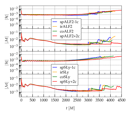
Figure 1: Top two panels show the Hamiltonian and momentum violations for all models of the ALF2 EoS. Bottom two panels similarly for the SLy EoS.

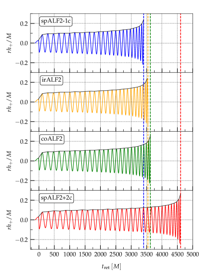
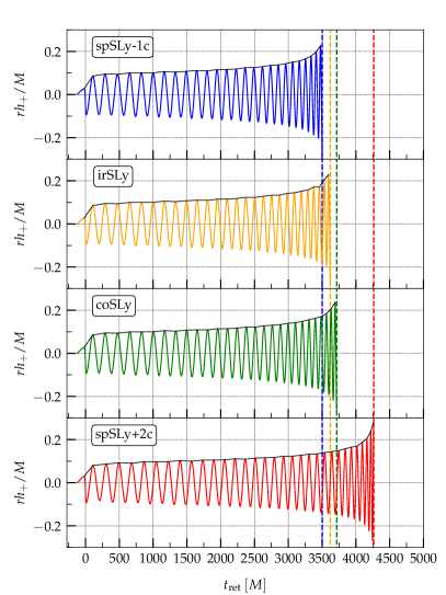
Figure 2: The strain of the plus polarization of the (2,2) GW mode for the ALF2 (left column) and the SLy (right column) EoSs. From top to bottom the binaries correspond to antialigned spinning, irrotational, corotating, and aligned spinning, respectively. Dashed vertical lines denote the time of the maximum amplitude $h=\sqrt{h_{+}^{2}+h_{\times}^{2}}$.

II.3 GW extraction

Extraction of GWs is performed using the complex Weyl scalar $\Psi_{4}$ and the fact that $\Psi_{4}=\ddot{h}_{+}-i\ddot{h}_{\times}$ Baumgarte and Shapiro (2010); Maggiore (2007); Ruiz et al. (2008). Expanding in terms of the spin-weighted spherical harmonics with spin weight $-2$

$$\Psi_{4}(t,r,\theta,\phi)=\sum_{\ell=2}^{\infty}\sum_{m=-\ell}^{\ell}\Psi_{4}^{\ell m}(t,r)\ _{-2}Y_{\ell m}(\theta,\phi)$$ (3)

and the strain $h=h_{+}-ih_{\times}$ of the GW will be

$$h(t,r,\theta,\phi)=\int_{-\infty}^{t}dt^{\prime}\int_{-\infty}^{t^{\prime}}dt^{\prime\prime}\ \Psi_{4}(t^{\prime\prime},r,\theta,\phi)\ .$$ (4)

For the 8 simulations performed here (with outer boundary at $x=y=z=1024$) we extract the GW coefficients $\Psi_{4}^{\ell m}(t,r)$ at seven radii, $R_{\rm gw}\in\{120,240,300,460,600,720,840\}$, in order to make sure that we have a waveform converged with radius. These coefficients are then expressed in terms of the retarded time $t_{\rm ret}=t-r_{\star}$ where $r_{\star}=r_{A}+2M\ln\left(r_{A}/(2M)-1\right)$ is the so-called tortoise coordinate. Here $r_{A}=\sqrt{A_{\rm gw}/(4\pi)}$ is the areal (Schwarzschild) coordinate and $A_{\rm gw}$ the proper area of a coordinate sphere of radius $R_{\rm gw}$.

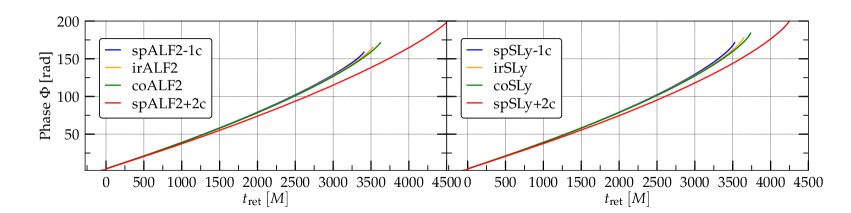
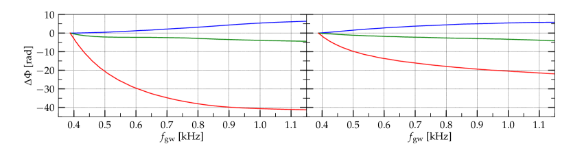
Figure 3: Left (right) column ALF2 (SLy) EoS. Top panels shows the phase evolution with respect to the retarded time while the bottom panels the phase difference between the irrotational and spinning models vs the GW frequency of the $(2,2)$ mode.

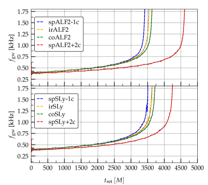
Figure 4: The gravitational wave frequency for the $l=2$, $m=2$ mode with respect to the retarded time for both the ALF2 (top panel) and SLy (bottom panel) EoSs. The black curves running through and practically overlapping with the colored ones are the fits using Eq. (8).

In order to calculate the strain, Eq. (4), we have to perform the double time integrations of the coefficients $\Psi_{4}^{\ell m}(t,r)$ and for that we follow the recipe of Ref. Reisswig and Pollney (2011) which strongly reduces spurious secular nonlinear drifts of the waveforms. First the Fourier transform $\Psi_{4}^{\ell m}(\omega,r)$ of $\Psi_{4}^{\ell m}(t,r)$ is calculated and then the strain coefficients are computed according to

$$h^{\ell m}(t,r)=-\frac{1}{2\pi}\int_{-\infty}^{+\infty}\frac{\Psi_{4}^{\ell m}(\omega,r)}{{\rm max}(\omega,\omega_{0})^{2}}e^{i\omega t}d\omega\ .$$ (5)

We choose $\omega_{0}=\Omega(t=0)$. Since in this work we simulate equal mass binaries and we are interested in the inspiral phase (up to merger) of identical stars, we will focus only at the $(\ell,m)=(2,2)$ mode. From now on we will denote this GW mode by $h=h_{+}^{22}-ih_{\times}^{22}$ and $\Phi$ the phase of $h$ at a specific radius, therefore we will write

$$h(t)=A(t)e^{i\Phi(t)}\ .$$ (6)

The GW angular frequency is defined as

$$\Omega_{\rm gw}=2\pi f_{\rm gw}=\frac{d\Phi}{dt}\ .$$ (7)

III Results

In Fig. 2 we plot the real part of the gravitational wave strain $h$ vs the retarded time for the 8 simulations of Table 2. The left column corresponds to the ALF2 models while the right to the SLy ones. From top to bottom we plot the spinning binaries with their spin antialigned with the orbital angular momentum, the irrotational, the corotating, and the aligned spinning ones. All waveforms are terminated at their peak amplitude (peak of $h=\sqrt{h_{+}^{2}+h_{\times}^{2}}$) that corresponds to the merger of the two neutron stars. The time of the peak amplitude of $h$ is not identical with the time of the peak amplitude of $h_{+}$, but very close to it. The so-called hang-up effect Campanelli et al. (2006), which was identified in BNS simulations Dietrich et al. (2015); Tsatsin and Marronetti (2013); Kastaun et al. (2013); Dietrich et al. (2017c); Ruiz et al. (2019) is clear in these waveforms. Comparing the irrotational waveforms of the two EoSs we see that the ALF2 binary merges earlier than the SLy one, in agreement with the fact that the tidal deformability of ALF2 is larger than the SLy one (see Table 4 for exact merger times and frequencies). Among the corotating models, the ALF2 merges earlier than the SLy even though its spin is much larger ($0.16$ vs $0.098$) implying that the combination of tidal effects and the larger orbital separation at merger (in the ALF2 case) dominate over spin effects. However, the model spALF2+2c merges later than spSLy+2c; therefore here the much higher spin of spALF2+2c overcomes the tidal interactions.

The effect of spin can be seen most clearly in Fig. 3 where the phase evolution of the gravitational wave signal is plotted vs the retarded time (top panels). At any given time the slope of the curves decreases with increasing aligned spin, with the steepest slope corresponding to the antialigned models (spALF2-1c, spSLy-1c) and the smaller for the aligned cases (spALF2+2c,spSLy+2c). A steeper phase slope (antialigned spins) leads to more bound systems, faster phase evolution, and thus earlier merger Damour (2001). In the bottom panels of Fig. 3 we plot the phase difference between the irrotational models and the spinning ones, $\Delta\Phi=\Phi_{\rm irrot}-\Phi_{\rm spin}$, vs $f_{\rm gw}$, the gravitational wave frequency of the (2,2) mode, in the LIGO band. The transition from retarded time to frequency has been accomplished using the relations shown in Fig. 4. Color lines represent raw data which exhibit a slight oscillatory behavior that is characteristic of the presence of eccentricity in the initial data. More accurate future evolutions will improve this artifact. In order to remove this residual eccentricity we perform fittings inspired by the post-Newtonian formalism Blanchet (2014),

$$2\pi f_{\rm gw}=\frac{1}{20M}z^{3}(c_{0}+c_{2}z^{2}+c_{3}z^{3}+c_{4}z^{4})$$ (8)

where $z=[(t_{c}-t)/(20M)]^{-1/8}$ and $t_{c}$ the coalescence time (maximum amplitude of the strain). The fitted curves (black lines in 4 that essentially coincide with the colored ones) are used in Fig. 3. By direct comparison of the two panels in the bottom row of Fig. 3 one can see that for small spins (antialigned (blue) and corotating (green)) the two EoSs yield small differences with respect to the irrotational case. For higher spins significant deviations from the irrotational models appear. In the post-Newtonian approximation one can identify the magnitude of the contributions due to different mechanisms, and to lowest order one can calculate the point particle (like a binary black hole), tidal, spin-orbit, spin-spin from self-interactions, and spin-spin from mutual interactions Dietrich et al. (2017c). In our case we find that, although small spins (depending also on the EoS) result to phase differences of the order of $\sim 5$ radians (in accordance with Ref. Dietrich et al. (2017c)), higher spins, can produce phase differences as large as $\sim 40$ radians within the $1\ {\rm KHz}$ band which are much larger than the tidal effects.

Table 4: Retarded time of the peak of the 2,2 mode as well as the corresponding frequencies for the 8 initial data configurations used in this work.

Name	$t_{\rm mrg}/M$	$f_{\rm mrg}$ [kHz]
spALF2-1c	$3405$	$1.62$
irALF2	$3536$	$1.72$
coALF2	$3630$	$1.75$
spALF2+2c	$4607$	$1.78$
spSLy-1c	$3495$	$1.47$
irSLy	$3630$	$1.98$
coSly	$3724$	$2.00$
spSLy+2c	$4262$	$2.15$

To see this, note that tidal contributions enter the GW phase at the 5PN order and are partially known up to 7.5PN Damour et al. (2012),

$$\phi_{{}_{T}} = \sum_{i=1}^{2}\kappa_{i}c_{{}_{\rm Newt}}^{i}x^{5/2}(1+c_{1}^{i}x+c_{3/2}^{i}x^{3/2}+c_{2}^{i}x^{2}$$ (9)

$$\qquad\qquad\qquad\ \ +c_{5/2}^{i}x^{5/2})\ ,$$

where $x=(M\pi f_{\rm gw})^{2/3}$ and the tidal deformability enters through the coefficient $\kappa_{1}=3\Lambda_{1}X_{1}^{4}X_{2}$ (similarly for $\kappa_{2}$). Here $X_{i}=M_{i}/M$, with $M_{i}$ the individual gravitational masses, and all the coefficients $c^{i}$ are functions of $X_{i}$ (see Damour et al. (2012)). Eq. 9 is plotted with solid lines in Fig. 5 for the two EoSs considered here.

In addition to the PN formula, tidal effects can be described based on numerical relativity simulations using the approximants derived in Refs. Kawaguchi et al. (2018); Dietrich et al. (2017b) either in the frequency or in the time domain. The basic idea of these approximants is to use binary black hole models in order to provide analytical closed-form expressions correcting the GW phase to include tidal effects. Here we use the approximant $\phi_{{}_{T}}^{{}_{\rm NR}}$ Dietrich et al. (2017b, 2019) referred to as NRTidal, which models the tidal effects in the time domain, Eq. 6. In Fig. 5 we plot $\phi_{{}_{T}}^{{}_{\rm NR}}$ (dashed lines) with respect to the frequency for the ALF2 and SLy models used in our simulation. As shown in the plot, the NRTidal phase shift between $f_{\rm gw}=0.4$ kHz and $f_{\rm gw}=1$ kHz is $\lesssim 8$ radian for ALF2 and $\lesssim 4$ radians for SLy. The aforementioned NRTidal phase shift for SLy (ALF2) is comparable with the phase shift due to spin for the SLy models spSLy-1c and coSly (ALF2 models spALF2-1c and coALF2) as shown in the bottom row of Fig. 3. For frequencies beyond the LIGO band, tidal effects still prevail over the spin for those cases.

However, for our highest spinning models the picture is completely different. At 1 KHz both the ALF2 and SLy EoSs develop a phase shift due to spin approximately 4 times larger than the one coming from tidal effects alone. Even for larger frequencies the shift due to spin in those cases will be larger than the corresponding one due to tidal effects, despite the fact that the slopes of the curves of Fig. 3 are smaller than those of Fig. 5 in the 1-2 KHz regime.

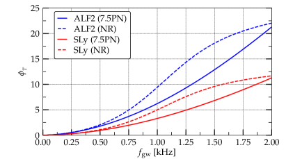
Figure 5: The 7.5PN tidal part (solid lines) of the GW phase for the two EoSs used in this work, together with the tidal approximant of Dietrich et al. Dietrich et al. (2017b) (dashed lines).

Another interesting feature of Fig. 3 is the fact that for a given EoS the phase difference of a spinning model with respect to the irrotational one does not scale linearly with the spin, a reminder of its nonlinear nature. For example although the antialigned and corotating ALF2 models have an absolute value of spin which is approximately half of the spALF2+2c model, the phase difference of the latter is approximately 8 times larger. For the SLy EoS the antialigned and corotating models have an absolute value of spin which is almost half of the spSLy+2c model, but the phase difference of the latter is approximately 4 times larger. Also by observing the antialigned and corotating ALF2, SLy models we can see that they produce similar phase shifts with respect to the irrotational case although their corresponding spins are $|\chi_{{}_{\rm ALF2}}|\approx 1.6|\chi_{{}_{\rm SLy}}|$. In other words for smaller spins softer EoSs produce the same phase shift as a stiffer one with a higher spin.

The power spectral density of the models we simulated together with the ZERO_DET_high_P aLIGO noise curve ($\sqrt{S_{n}(f)}$) are plotted in Fig. 6. Spin effects are clearly not distinguishable on this plot.

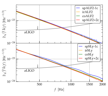
Figure 6: GW spectra of the ALF2 and SLy numerical waveforms at $50$ Mpc, and aLIGO ZERO_DET_high_P noise curve (thick grey lines).

IV Discussion

In this work we performed long-term inspiral simulations of irrotational and highly spinning binary neutron stars using the Illinois grmhd code in an effort to assess the importance of high spin. We used two EoSs representing NSs of different compactions and three different spins in order to compare the phase evolution with respect to the irrotational case. Our spinning models range from binaries with a spin $\sim 0.32$ aligned with the orbital angular momentum, to antialigned binaries with a spin of $\sim-0.17$, all of them of equal mass. We employed high resolution with our finest grid spacing $\Delta x=98$ m, motivated by the study of Kiuchi et al. (2017). We find that our highest spinning binary exhibit a phase difference of $\sim 40$ radians with respect to the irrotational one. This shift grows nonlinearly with the spin and depends on the EoS too. Our findings indicate in full general relativity that the effect of moderate to high spin in the inspiral can be larger than the tidal effects alone, even when the rotation of the stars is far from their Keplerian limit. The dephasing due to spin is in accordance with post-Newtonian analysis Harry and Hinderer (2018), and this work underlines the importance of taking it into account for more reliable GW data analysis.

Despite the fact that our calculations employ among the highest resolutions adopted in numerical relativity simulations of inspiraling binary neutron stars to-date, we find that our irrotational models complete about 0.5-1 fewer orbits when compared to previous studies. This would suggest a maximum phase error of about $4\pi\approx 12.6$ radians. To obtain a better handle on the phase error in our calculations, and test whether a phase difference between a spin 0.32 and spin 0 binary can be as high as $\sim 40$ radians, we used the IMRPhenomD approximant Khan et al. (2016) as implemented in PyCBC Biwer et al. (2019) to construct time domain binary black hole waveforms. The results suggests that for a total mass of 2.72$M_{\odot}$, starting 400 Hz and ending at $1\ {\rm kHz}$, the phase difference between an equal-mass, non-spinning binary black hole and a binary black hole with dimensionless spin parameters $0.32$ is $\sim$ 25 radians. This suggests that the phase difference of $\sim 40$ radians between our highest spin and irrotational ALF2 cases is likely an overestimate, indicating that the phase error in our calculations is possibly as high as $\sim 15$ radians for the ALF2 EoS. A similar calculation for the spins we treat in the SLy EoS, shows a phase difference in the binary black hole case of $\sim 15$ radians, suggesting an error in our SLy phase difference calculations possibly as high as $5$ radians. Regardless, the main result of our work is intact: the effect of spin in the inspiral of a binary neutron star system can be larger than the tidal effects and depends of the EoS, hence its inclusion in the GW data analysis is important. While this result may sound obvious, we point out that the spacetime outside a rotating NS is not Kerr, and hence one cannot a-priori expect that spin effects in binary neutron stars will be the same as those in binary black holes. Thus, our calculations provide an explicit demonstration that spin effects can be very important during the inspiral of a binary neutron star.