On the Parallelization of Triangular Decomposition of Polynomial Systems

Abstract.

We discuss the parallelization of algorithms for solving polynomial systems symbolically by way of triangular decomposition. Algorithms for solving polynomial systems combine low-level routines for performing arithmetic operations on polynomials and high-level procedures which produce the different components (points, curves, surfaces) of the solution set. The latter “component-level” parallelization of triangular decompositions, our focus here, belongs to the class of dynamic irregular parallel applications. Possible speed-up factors depend on geometrical properties of the solution set (number of components, their dimensions and degrees); these algorithms do not scale with the number of processors.
In this paper we combine two different concurrency schemes, the fork-join model and producer-consumer patterns, to better capture opportunities for component-level parallelization. We report on our implementation with the publicly available BPAS library. Our experimentation with 340 systems yields promising results.

1. Introduction

In linear algebra, stencil computations, sorting algorithms, fast Fourier transform and other standard kernels in scientific computing, opportunities for parallel computations often come from either a divide-and-conquer scheme, with concurrent recursive calls, or a for-loop nest where some iterations can be executed concurrently.

In the case of non-linear polynomial algebra, opportunities for parallel computations can be categorized between low-level routines for performing arithmetic operations on polynomials and high-level procedures for algebraic and geometric computations. Many of those low-level routines follow patterns that are similar to standard kernels in scientific computing and their parallelization has been well studied for both dense and sparse polynomials (Monagan and Pearce, 2009, 2010; Gastineau and Laskar, 2013, 2015).

The parallelization of high-level procedures for algebraic and geometric computations received much attention in the 80’s and 90’s, see (Buchberger, 1987; Saunders et al., 1989; Bündgen et al., 1994; Faugere, 1994; Attardi and Traverso, 1996). More recently in (Maza and Xie, 2007), two of the current authors consider the parallelization of triangular decompositions of polynomial systems.

Triangular decomposition—a symbolic method for solving systems of polynomial equations—uses algebraic techniques to split the solution space into geometric components (i.e. points, curves, surfaces, etc.). For those techniques, opportunities for parallel computations depend only on the geometry of the input system and may vary from none to many. Moreover, when such opportunities are present the workload between tasks may be largely unbalanced.

1.1. Problem Statement

The preliminary work reported in (Maza and Xie, 2007) does not cover all opportunities for concurrent/parallel processing of component-level, i.e. high-level, procedures in triangular decompositions of polynomial systems, leaving open the full question of possibilities for component-level parallelism, both in terms of algorithm scheme and implementation techniques. The tests also used only a few examples computed modulo a prime number instead of using rational number coefficients, increasing the number of the components and hence the possible speed-up factors with respect to serial.

To stress the importance of the proposed question one can make the following observation. In computer algebra systems like Maple only low-level routines for polynomial arithmetic use multithreaded parallelism while high-level procedures, such as Maple’s solve command (for solving systems of systems of polynomial or differential equations symbolically) execute serial code.

1.2. Contributions

We make use of both the fork-join model and the pipeline pattern (via asynchronous producer-consumer) to exploit opportunities for parallelism in the component-level of triangular decomposition. To our knowledge, this is the first time that the producer-consumer model is used in a high-level algorithm in symbol computation.

Triangular decompositions have two important features: the necessity of removing redundant (that is, superfluous) components and the possibility of avoiding the computation of degenerate components. These features lead to different algorithm variants that we call Level vs. Bubble (two different strategies for removing redundant components), and Lazard-Wu vs. Kalkbrener decompositions (that is whether or not degenerate components may be ignored).

These different algorithm variants combined with three degrees of parallelism granularity (fine-grained, coarse-grained, and serial) lead to 12 different configurations of our implementation. The parallelism in our implementation is achieved using the standard C++11 thread support library as well as the Cilk extension of C/C++.

We test the various configurations of our implementation by considering a suite of approximately 3000 real-world polynomial systems. These systems, provided by MapleSoft (the company developing Maple), come from a combination of actual user data, bug reports, and the scientific literature. We have obtained speed-up factors up to 8 on a 12-core machine. We highlight that the underlying polynomial arithmetic is performed serially since we focus on component-level parallelization of triangular decomposition. Among these configurations we find that the Bubble variant admits more parallelism than the Level variant while solving in the Kalkbrener sense admits more parallelism than solving in the Lazard-Wu sense. By this, we mean that Bubble and Kalkbrener benefit from parallelism more often and to a higher a degree.

1.3. Structure of the Paper

Following a presentation of the mathematical background for triangular decomposition in Section 2, Section 3 reviews the main features of triangular decomposition computations. Section 4 discusses opportunities for concurrent execution in these computations. Section 5 reports on their implementation, and Section 6 presents our experimentation. Section 7 highlights directions for future work.

2. Algebraic background

Section 2.3 focuses on a celebrated algebraic construction by which computations can split when solving polynomial systems, thus bringing opportunities for parallel computations, though not necessarily balanced in terms of workload. This construction, called the D5 Principle after its authors (Della Dora et al., 1985) relies on the well-known Chinese remainder theorem, reviewed in Section 2.2.

2.1. Solving polynomial systems incrementally

An informal sketch of the top-level procedure considered in this paper is given by Algorithm 1, while a more formal version is stated as Algorithm 2. For a finite set $F$ of polynomial equations, the function SolveSystemIncrementally$(F)$ returns the common solutions of the members of $F$ described as a finite set of components $T_{1},\ldots,T_{e}$. By a component, we mean a set of polynomial equations with remarkable algebraic properties; see Section 3 for more details. Algorithm 1 proceeds by incrementally solving one equation after another against each component produced by the previously solved equations. The core routine is SolveOneEquation$(p,T)$ which solves the polynomial equation $p$ against the component $T$, that is, finding the solutions of $p$ that are also solutions of $T$.

Input: a finite set $F$ of polynomial equations

Output: a set of components such that their union is the solution set of $F$

if $|F|==0$ then return $[\{\}]$;

Choose a polynomial $p\in F$;

for $T{\bf\ in\ }\mbox{{\sf SolveSystemIncrementally}$(F\setminus\{p\})$}$ do

       yield $\mbox{{\sf SolveOneEquation}$(p,T)$};$

Algorithm 1 SolveSystemIncrementally$(F)$

Example 2.1.

Consider the polynomial system:

$$\left\{\begin{array}[]{rl}f_{1}:&x^{3}-3x^{2}+2x=0\\ f_{2}:&2yx^{2}-x^{2}-3yx+x=0\\ f_{3}:&zx^{2}-zx=0\end{array}\right.$$

Calling SolveOneEquation$(f_{1},\varnothing)$ yields $\{f_{1}\}$ since $f_{1}$ is “simple enough” to define a component on its own, namely the points $(x,y,z)$ satisfying $x^{3}-3x^{2}+2x=0$.

Consider now the call SolveOneEquation$(f_{2},\{f_{1}\})$. Note that $f_{1}$ and $f_{2}$ rewrite respectively as $x(x-1)(x-2)=0$ and $x((2x-3)y-x+1)=0$. Clearly $x=0$ is a common solution while, for $x=1$ and $x=2$, the equation $f_{2}$ simply becomes $y=0$ and $y=1$, respectively. Therefore, SolveOneEquation$(f_{2},\{f_{1}\})$ returns 3 components:

$$T_{1}:\left\{\begin{array}[]{r}x=0\end{array}\right.,\>\>\>\>T_{2}:\left\{\begin{array}[]{r}y=0\\ x=1\end{array}\right.\>\>{\rm and}\>\>T_{3}:\left\{\begin{array}[]{r}y=1\\ x=2\end{array}\right.$$

Next, we need to compute SolveOneEquation$(f_{3},T_{i})$, for $1\leq i\leq 3$. We observe that $f_{3}$ satisfies both $T_{1}$ and $T_{2}$, hence the first two calls return $T_{1}$ and $T_{2}$. For the third one, we note that $f_{3}$ simply becomes $z=0$ at $(y,x)=(1,2)$. Finally, SolveSystemIncrementally$(\{f_{1},f_{2},f_{3}\})$ returns the following 3 components:

$$T_{1}:\left\{\begin{array}[]{r}x=0\end{array}\right.,\>\>\>\>T_{2}:\left\{\begin{array}[]{r}y=0\\ x=1\end{array}\right.\>\>{\rm and}\>\>T_{3}:\left\{\begin{array}[]{r}z=0\\ y=1\\ x=2\end{array}\right.$$

While the previous example shows an opportunity for parallel computations, namely computing SolveOneEquation$(f_{3},T_{i})$, for $1\leq i\leq 3$ in parallel, it hides a major difficulty: possible unbalanced work. Here is an illustrative example of this latter fact.

Example 2.2.

Consider the polynomial system:

$$\left\{\begin{array}[]{rl}f_{1}:&\left(x-1\right)x=0\\ f_{2}:&x\left({y}^{n}-x\right)+\left(x-1\right)\left(y-x\right)=0\\ f_{3}:&\left({y}^{n+1}+1\right)z-x=0\end{array}\right.$$

where $n\geq 2$ is integer. Calling SolveOneEquation$(f_{1},\varnothing)$ yields $\{f_{1}\}$, as in Example 2.1. Now, SolveOneEquation$(f_{2},\{f_{1}\})$ returns 3 components by means of simple calculations not detailed here:

$$T_{1}:\left\{\begin{array}[]{r}\sum_{i=0}^{n-1}y^{i}=0\\ x=1\end{array}\right.,\>\>\>\>T_{2}:\left\{\begin{array}[]{r}y=1\\ x=1\end{array}\right.\>\>{\rm and}\>\>T_{3}:\left\{\begin{array}[]{r}y=0\\ x=0\end{array}\right.$$

Next, we compute SolveOneEquation$(f_{3},T_{i})$, for $1\leq i\leq 3$. Elementary calculations not reported here produce 3 components:

$$T_{1}:\left\{\begin{array}[]{r}(y+1)z+x=0\\ \sum_{i=0}^{n-1}y^{i}=0\\ x=1\end{array}\right.,\>\>\>\>T_{2}:\left\{\begin{array}[]{r}2z+1=0\\ y=1\\ x=1\end{array}\right.\>\>{\rm and}\>\>T_{3}:\left\{\begin{array}[]{r}z=0\\ y=0\\ x=0\end{array}\right.$$

One should observe that the first equation in $T_{2}$ (resp. $T_{3}$) is obtained by evaluating $f_{3}$ at $(x,y)=(1,1)$ (resp. $(0,0)$), which is a trivial operation, the cost of which can be considered constant. Now, one should notice that the first equation in $T_{1}$ is not $f_{3}$ itself, but $(y+1)z+x=0$. This simplification requires dividing $y^{n+1}+1$ by $\sum_{i=0}^{n-1}y^{i}$, which, for $n$ large enough, is arbitrarily expensive. As a result, the work load in SolveOneEquation$(f_{3},T_{i})$, for $1\leq i\leq 3$, can be arbitrarily unbalanced.

Example 2.2 shows that parallelizing the for-loop in Algorithm 1 may not bring much benefit. Nevertheless, this does not imply that, for other examples, it should not be attempted. In fact, the call SolveOneEquation$(p,T)$ itself has various opportunities for concurrency. Combined with that Algorithm 1, many practical examples, but not all, may benefit from a careful implementation of concurrency, as explained in Sections 4 and 5.

2.2. The Chinese remainder theorem

One of the most fundamental results in algebra is the Chinese remainder theorem (CRT). Let $m_{1}$ and $m_{2}$ be two relatively prime numbers, so that there exist integers $u_{1},u_{2}$ satisfying $u_{1}m_{1}+u_{2}m_{2}=1$. The CRT states that the residue class ring ${\mbox{${\mathbb{Z}}$}}/(m_{1}\,m_{2})$ is isomorphic to the direct product of the residue class rings ${\mbox{${\mathbb{Z}}$}}/m_{1}$ and ${\mbox{${\mathbb{Z}}$}}/m_{2}$, denoted as ${\mbox{${\mathbb{Z}}$}}/m_{1}\otimes{\mbox{${\mathbb{Z}}$}}/m_{2}$, which writes:

(1) $${\mbox{${\mathbb{Z}}$}}/(m_{1}\,m_{2})\ \ \equiv\ \ {\mbox{${\mathbb{Z}}$}}/m_{1}\otimes{\mbox{${\mathbb{Z}}$}}/m_{2}.$$

In the above direct product, elements are pairs of residues $(r_{1},r_{2})$ with $r_{i}\in{\mbox{${\mathbb{Z}}$}}/m_{i}$ and operations (addition, subtraction, multiplication) are performed component-wise. That is, $(r_{1},r_{2})+(s_{1},s_{2})=(r_{1}+s_{1},r_{2}+s_{2})$ and $(r_{1},r_{2})\times(s_{1},s_{2})=(r_{1}\times s_{1},r_{2}\times s_{2})$ both hold for all $r_{i},s_{i}\in{\mbox{${\mathbb{Z}}$}}/m_{i}$, for $1\leq i\leq 2$. The isomorphism stated in Equation (1) is a one-to-one map $\Phi$ by which:

the image of $r\in{\mbox{${\mathbb{Z}}$}}/(m_{1}\,m_{2})$ is $(r\mod{m_{1}},r\mod{m_{2}})$,

the preimage of $(r_{1},r_{2})\in{\mbox{${\mathbb{Z}}$}}/m_{1}\otimes{\mbox{${\mathbb{Z}}$}}/m_{2}$ is $(r_{1}m_{1}u_{1}+r_{2}m_{2}u_{2})\mod{m_{1}\,m_{2}}$, and

the image of a sum (resp. product) is the sum (resp. product) of the images, that is, $\Phi(r+s)=\Phi(r)+\Phi(s)$ and $\Phi(r\times s)=\Phi(r)\times\Phi(s)$. These properties imply that

any computation (i.e. combination of additions, subtractions, multiplications) in ${\mbox{${\mathbb{Z}}$}}/(m_{1}\,m_{2})$ can be transported to ${\mbox{${\mathbb{Z}}$}}/m_{1}\otimes{\mbox{${\mathbb{Z}}$}}/m_{2}$, where

computations split into two “independent coordinates”, one in ${\mbox{${\mathbb{Z}}$}}/m_{1}$ and one in ${\mbox{${\mathbb{Z}}$}}/m_{2}$, which can be considered concurrently.

The CRT generalizes in many ways. First, with several pairwise relatively prime integers $m_{1},m_{2},\ldots,m_{e}$, yielding the following:

${\mbox{${\mathbb{Z}}$}}/(m_{1}m_{2}\cdots m_{e})\ \ \equiv\ \ {\mbox{${\mathbb{Z}}$}}/m_{1}\otimes{\mbox{${\mathbb{Z}}$}}/m_{2}\otimes\cdots\otimes{\mbox{${\mathbb{Z}}$}}/m_{e}$

Second, with polynomials instead of integers. For this second case and to be precise, consider the field ${\mathbb{Q}}$ of rational numbers and the ring of univariate polynomials in $x$ over ${\mathbb{Q}}$, denoted by ${\mbox{${\mathbb{Q}}$}}[x]$. For non-constant polynomials $p_{1},p_{2},\ldots,p_{e}$ that are relatively prime (meaning here that any two polynomials $p_{i},p_{j}$, for $1\leq i<j\leq e$ have no common factors, except rational numbers) we have the following isomorphism:

(2) $${{\mbox{${\mathbb{Q}}$}}[x]}/(p_{1}p_{2}\cdots p_{e})\ \ \equiv\ \ {{\mbox{${\mathbb{Q}}$}}[x]}/p_{1}\otimes{{\mbox{${\mathbb{Q}}$}}[x]}/p_{2}\otimes\cdots\otimes{{\mbox{${\mathbb{Q}}$}}[x]}/p_{e}$$

When the polynomials $p_{1},p_{2},\ldots,p_{e}$ are irreducible, then each of ${{\mbox{${\mathbb{Q}}$}}[x]}/p_{1}$, ${{\mbox{${\mathbb{Q}}$}}[x]}/p_{2}$, …, ${{\mbox{${\mathbb{Q}}$}}[x]}/p_{e}$ is in fact a field. In such case, the residue class ring ${{\mbox{${\mathbb{Q}}$}}[x]}/(p_{1}p_{2}\cdots p_{e})$ is a direct product of fields, an algebraic structure with interesting properties. For instance, if $e=2$, $p_{1}=x^{2}-2$ and $p_{2}=x^{2}-3$, then ${{\mbox{${\mathbb{Q}}$}}[x]}/p_{1}$ and ${{\mbox{${\mathbb{Q}}$}}[x]}/p_{2}$ are the field extensions ${\mbox{${\mathbb{Q}}$}}(\sqrt{2})$ and ${\mbox{${\mathbb{Q}}$}}(\sqrt{3})$. Those latter fields consist of all numbers obtained by adding, multiplying rational numbers together with $\sqrt{2}$ and $\sqrt{3}$, respectively.

When the polynomials $p_{1},p_{2},\ldots,p_{e}$ are square-free then each of ${{\mbox{${\mathbb{Q}}$}}[x]}/p_{1}$, ${{\mbox{${\mathbb{Q}}$}}[x]}/p_{2}$, …, ${{\mbox{${\mathbb{Q}}$}}[x]}/p_{e}$ is in fact a direct product of fields (DPF). (This claim directly follows from the previous paragraph.)

Now, a third generalization of the CRT is as follows. For non-constant pairwise relatively prime polynomials $f_{1},f_{2},\ldots,f_{e}$ in ${\mbox{${\mathbb{K}}$}}[x]$, where ${\mathbb{K}}$ is a DPF, we have the following isomorphism:

(3) $${{\mbox{${\mathbb{K}}$}}[x]}/(p_{1}p_{2}\cdots p_{e})\ \ \equiv\ \ {{\mbox{${\mathbb{K}}$}}[x]}/p_{1}\otimes{{\mbox{${\mathbb{K}}$}}[x]}/p_{2}\otimes\cdots\otimes{{\mbox{${\mathbb{K}}$}}[x]}/p_{e}$$

2.3. The D5 principle

It follows from the discussion above that DPFs generalize fields. Moreover, square-free polynomials can be used to build extensions of DPFs. Hence, one can “almost” work with DPFs as if they were fields. The “almost” comes from the fact that DPFs have zero-divisors while fields, by definition, do not. Returning to the example

${{\mbox{${\mathbb{Q}}$}}[x]}/(p_{1}p_{2})\ \ \equiv\ \ {{\mbox{${\mathbb{Q}}$}}[x]}/p_{1}\otimes{{\mbox{${\mathbb{Q}}$}}[x]}/p_{2}$,

with $p_{1}=x^{2}-2$ and $p_{2}=x^{2}-3$, we observe that $p_{2}$ (as an element of ${{\mbox{${\mathbb{Q}}$}}[x]}/(p_{1}p_{2})$) is mapped to $(p_{2}\mod{p_{1}},p_{2}\mod{p_{2}})=(1,0)$, since $p_{2}=1+p_{1}$. Now observe that $(1,0)\times(0,1)=(0,0)$ holds. Hence $(1,0),(0,1)$ are two non-zero elements of ${{\mbox{${\mathbb{Q}}$}}[x]}/p_{1}\otimes{{\mbox{${\mathbb{Q}}$}}[x]}/p_{2}$, with zero as product. That is, $(1,0),(0,1)$ are zero-divisors.

Zero-divisors do not have multiplicative inverses and, thus, are an obstacle to certain operations. For instance, consider two univariate polynomials $a,b\in{\mbox{${\mathbb{L}}$}}[y]$, with $b$ non-constant, over a direct product of fields ${\mathbb{L}}$. Then, the polynomial division of $a$ by $b$ is uniquely defined provided that the leading coefficient of $b$ is invertible, that is, not a zero-divisor. Indeed, every non-zero element in a DPF is either invertible or a zero-divisor.

The D5 principle (Della Dora et al., 1985) states that computations in ${\mbox{${\mathbb{L}}$}}[y]$ can be performed as if ${\mathbb{L}}$ was a field, provided that, when a zero-divisor is encountered, computations split into separate coordinates, following an isomorphism, like the one given by Equation (2). We shall explain more precisely what this means.

We assume that ${\mathbb{L}}$ is of the form ${\mbox{${\mathbb{K}}$}}[x]/p$ where $p$ is a square-free non-constant polynomial and ${\mathbb{K}}$ is either a field (e.g. ${\mathbb{Q}}$) or another DPF. Returning to the polynomial division of $a$ by $b$, we should decide whether $h$, the leading coefficient of $b$, is invertible or not. Note that $h$ is a polynomial in ${\mbox{${\mathbb{K}}$}}[x]$. Thus, the invertibility of $h$ modulo $p$ can be decided by applying the extended Euclidean algorithm (to which we recursively apply the D5 principle, in case ${\mathbb{K}}$ is itself a DPF) in ${\mbox{${\mathbb{K}}$}}[x]$, with $h$ and $p$ as input. This produces three polynomials $u,v,g$, with $g\neq 0$, such that $u\,h\,+v\,p\ =\ g.$

First, assume that the leading coefficient of $g$ is invertible in ${\mathbb{K}}$. Then, $g$ is a greatest common divisor (GCD) of $h$ and $p$. Two cases arise:

if $g$ is a constant of ${\mathbb{K}}$ (that is, $g$ has degree zero as a polynomial in ${\mbox{${\mathbb{K}}$}}[x]$) then $ug^{-1}h\equiv 1\,\mod{p}$ holds and we have proved that $h$ is invertible;

if $g$ is not constant (that is, $g$ has a positive degree in $x$) then, since $p$ is square-free resulting in $g$ and $\nicefrac{{p}}{{g}}$ being relatively prime, CRT gives us,

${\mbox{${\mathbb{L}}$}}\ \ \equiv\ \ {\mbox{${\mathbb{K}}$}}[x]/g\,\otimes{\mbox{${\mathbb{K}}$}}[x]/\frac{p}{g}$,

It follows that either $h$ is invertible or computations split. In the latter case, computations resume independently on each coordinate.

Second, assume that the leading coefficient of $g$ is not invertible in ${\mathbb{K}}$. Then, reasoning by induction, the DPF ${\mathbb{K}}$ can be replaced by a direct product so that, here again, computations are performed independently on each coordinate.

3. The Triangularize algorithm

The Triangularize algorithm is a procedure for solving systems of polynomial equations incrementally. Hence, it follows the algorithmic pattern discussed in Section 2.1. The Triangularize algorithm was first proposed in (Moreno Maza, 2000) and substantially improved in (Chen and Maza, 2012). An extension to systems of polynomial equations and inequalities is presented in (Li et al., 2009).

The components produced by the Triangularize algorithm are called quasi-components: they are represented by families of polynomials with remarkable properties called regular chains. We refer to (Chen and Maza, 2012) for a formal presentation, while Section 3.1 describes only the properties relevant to the concurrent execution of Triangularize.

3.1. Regular chains

Let ${\mathbb{L}}$ be a direct product of fields (DPF) as defined in Section 2.3. Thus, ${\mathbb{L}}$ is of the form ${\mbox{${\mathbb{K}}$}}[x]/p$ where $p$ is a square-free non-constant polynomial and ${\mathbb{K}}$ is either a field (e.g. ${\mathbb{Q}}$) or another DPF.

If follows that any DPF ${\mathbb{L}}$ can be given by a sequence of multivariate polynomials $T=p_{1}(x_{1}),p_{2}(x_{1},x_{2}),\ldots,p_{n}(x_{1},x_{2},\ldots,x_{n})$ with coefficients in a field ${\mbox{${\mathbb{L}}$}}_{0}$, such that, for $1\leq i\leq n$, we have:

$p_{i}$ is a square-free non-constant polynomial in ${\mbox{${\mathbb{L}}$}}_{i-1}[x_{i}]$,

the leading coefficient $h_{i}$ of $p_{i}$ is regular with respect to ${\mbox{${\mathbb{L}}$}}_{i-1}$, i.e. invertible in ${\mbox{${\mathbb{L}}$}}_{i-1}$, and

${\mbox{${\mathbb{L}}$}}_{i}:={\mbox{${\mathbb{L}}$}}_{i-1}[x_{i}]/p_{i}$ and ${\mbox{${\mathbb{L}}$}}_{n}={\mbox{${\mathbb{L}}$}}$. Two cases are of practical importance. First, if ${\mbox{${\mathbb{L}}$}}_{0}={\mbox{${\mathbb{Q}}$}}$, then any point $(z_{1},z_{2},\ldots,z_{n})$ with complex number coordinates satisfying

$p_{1}(z_{1})=p_{2}(z_{1},z_{2})=\cdots=p_{n}(z_{1},z_{2},\ldots,z_{n})=0$,

is called a solution of $T$; the set of those solutions is denoted by $V(T)$: this is a finite set and $T$ is called zero-dimensional. Second, if ${\mbox{${\mathbb{L}}$}}_{0}$ is a field of rational functions with variables $t_{1},\ldots,t_{d}$, then any point $(t_{1},\ldots,t_{d},z_{1},\ldots,z_{n})$ with complex number coordinates satisfying for $1\leq i\leq n$:

$p_{i}(t_{1},\ldots,t_{d},z_{1},\ldots,z_{i})=0\ {\rm and}\ h_{i}(t_{1},\ldots,t_{d},z_{1},\ldots,z_{i-1})\neq 0$,

is called a solution of $T$; the set of those solutions is denoted by $W(T)$ and called a quasi-component: this set has dimension $d$. In either case, the sequence $T$ of polynomials is called a regular chain.

3.2. The main procedure and its core routines

Algorithm 2 states the top-level procedure of the Triangularize algorithm. Let us denote by $f_{1},f_{2},\ldots,f_{m}$ the polynomials in $F$ and by $x_{1},x_{2},\ldots,x_{n}$ their variables. Clearly, computations are essentially done by the core routine Intersect, which corresponds to the SolveOneEquation routine from Algorithm 1; naturally, Triangularize itself corresponds to SolveSystemIncrementally. For a polynomial $p\in{\mbox{${\mathbb{Q}}$}}[x_{1},x_{2},\ldots,x_{n}]$ and a regular chain $T$ given by polynomials from ${\mbox{${\mathbb{Q}}$}}[x_{1},x_{2},\ldots,x_{n}]$, the function call Intersect$(p,T)$ returns regular chains $T_{1},T_{2},\ldots,T_{e}$ so that the union $W(T_{1})\cup W(T_{2})\cup\cdots\cup W(T_{e})$ is an approximation of the intersection $W(T)\cap V(p)$. This approximation is, in fact, very sharp and this is why Triangularize$(F)$ is capable of producing regular chains such that the union of their zero sets is exactly equal to the zero set of $F$, denoted $V(F)$.

Input: a finite set of polynomials $F$

Output: a set of regular chains such that the union of their zero sets is $V(F)$

if $|F|==0$ then return $[\{\}]$;

Choose a polynomial $p\in F$;

for $T{\bf\ in\ }\mbox{{\sf Triangularize}$(F\setminus\{p\})$}$ do

       yield Intersect$(p,T)$;

      

Algorithm 2 Triangularize$(F)$

During the execution of Intersect$(p,T)$, two mechanisms lead computations to split into different cases:

case distinctions of the form “either $a=0$ or $a\neq 0$”, where $a$ is a polynomial by which one wants to divide another polynomial, like in $ax=b$ when solving for $x$.

Case distinctions resulting from the application of the D5 principle, as described in Section 2.3. Case distinctions of this latter type are generated by Regularize, a core routine of Triangularize. Figure 1, taken from (Chen and Maza, 2012), displays the “depends on” graph of the main routines of Triangularize.

Figure 1. The flow graph of the Triangularize algorithm.

3.3. Removal of the redundant components

As we have seen with Examples 2.1 and 2.2, computing Intersect$(p,T)$ often leads to case distinctions of the form: either $a=0$ or $a\neq 0$. Those are likely to produce components that are redundant, while not being incorrect. Here’s a trivial example. Consider $F:=\{f_{1},f_{2}\}$ with $f_{1}:yx+y=0$ and $f_{2}:y=0$. Intersect$(f_{1},\varnothing)$ yields two regular chains $T_{1},T_{2}$ with $T_{1}:y=0$ and $T_{2}:x+1=0$. Then, Intersect$(f_{2},T_{1})$ yields $T_{1}$ itself while Intersect$(f_{2},T_{2})$ yields $T_{3}$, with $T_{3}:x+1=0,y=0$. Clearly, $T_{3}$ is a special case of $T_{1}$, that is, we have $W(T_{3})\subseteq W(T_{1})$ and $T_{3}$ is redundant.

Precisely, letting $T_{1},T_{2},\ldots,T_{e}$ be the output regular chains of Triangularize$(F)$ in Algorithm 2, regular chain $T_{i}$ is redundant when:

$W(T_{i})\subseteq W(T_{1})\cup\cdots\cup W(T_{i-1})\cup W(T_{i+1})\cup\cdots\cup W(T_{e})$.

There exist criteria and algorithmic procedures for testing whether a regular chain is redundant or not. However, applying those criteria and procedures can be very computationally expensive. As a result, one should carefully consider when to attempt performing those computations. Two strategies are meaningful here:

barrier::

test for redundant components on every output returned by a call to Triangularize, including recursive calls;

barrier-free::

test for redundant components only on the final output returned by Triangularize$(F)$.

With the barrier strategy, all calls of the form Intersect$(f_{i},T)$ must complete before starting to execute the calls of the form Intersect$(f_{i+1},T^{\prime})$, for $1\leq i\leq m$, where $F:=\{f_{1},f_{2},\ldots,f_{m}\}$ is the input of Triangularize. For this reason, this strategy computes the solution level-by-level, hence we call it Level in subsequent sections. With the barrier-free approach, particularly when using parallelization, some calls of the form Intersect$(f_{i+1},T^{\prime})$ may be executed before completing all calls of the form Intersect$(f_{i},T^{\prime})$. We call this method Bubble in subsequent sections because it allows components to “bubble up” to higher levels of the recursion in Triangularize. Section 4 considers the parallelization and implementation details of these two strategies and redundant component removal.

3.4. Computing generic solutions

Another major feature of the Triangularize algorithm leads to different strategies and should be carefully considered towards performance in both serial and concurrent execution. This feature deals with the “scope” of the solution set. To be precise, it is possible to limit the computations of Triangularize to the so-called generic solutions. We refer again to (Chen and Maza, 2012) for a formal presentation and we shall simply use an illustrative example here. Consider the input system $F$ with the unique equation $ax=b$ with the intention of solving for $x$. Triangularize$(F)$ returns two regular chains $T_{1}:ax=b$ and $T_{2}:a=0,b=0$. The first one encodes all solutions for which $a\neq 0$ holds. “Generically” (say, by randomly picking a value of $a$) we have $a\neq 0$. Hence $T_{1}$ encodes all generic solutions while $T_{2}$ correspond to the non-generic ones, also called degenerate solutions.

The Triangularize algorithm can be executed in two modes, the names of which are from mathematicians who have studied strategies corresponding to those modes:

Kalkbrener::

non-generic solutions are likely not computed,

Lazard-Wu::

all solutions (generic or not) are computed.

The former mode is derived from the latter by a tree pruning technique. To clarify this, we can understand the Triangularize algorithm to be performing a breadth-first search (BFS) of a tree of intersections of polynomials and regular chains. See Figure 2 for an example of this. The Lazard-Wu decomposition finds all paths of the tree that yield solutions of the input system. The Kalkbrener decomposition, however, cuts off branches of the tree for which the height of a regular chain, i.e., the number of polynomials in the chain, exceeds a certain bound. In this way, paths of the tree that exceed the height bound are “pruned”. In the analogy to BFS, Kalkbrener decomposition is similar to Dijkstra’s algorithm for finding optimal paths (where height is analogous to edge weight). For polynomial systems that are computationally expensive to solve, it is often the case that the Kalkbrener mode can use much less computing resources (CPU time, memory) than the Lazard-Wu mode.

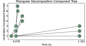
Figure 2. A tree of components from the splitting of computations through the TriangularizeLevel algorithm run on a system of 2 polynomials in 2 variables. The label on each node represents the component’s dimension while the grid lines indicate the time at which each level was complete.

4. Exploiting Concurrency in Triangular Decomposition

The Triangularize algorithm is highly complex, both in time-complexity and in conceptual complexity. This can seen from the flow graph in Figure 1 above. While all of the subroutines are greatly important to the algorithm we do not detail them here; for a more complete description see (Chen and Maza, 2012). Here we illustrate how Triangularize and its subroutines hold opportunities for parallelism from an algorithmic point of view.

We begin in Section 4.1 by discussing the concurrency paradigms applicable to the Triangularize algorithm. The parallelization of the removal of redundant components and the Triangularize algorithm itself are then discussed in Sections 4.2 and 4.3, respectively.

4.1. The fork-join model, generators, and the producer-consumer pattern

There are many patterns common to parallel processing, algorithms, and programming; fork-join, map-reduce, and the stencil pattern are notable. Fork-join is an idiomatic pattern for parallel processing at the heart of many concurrency platforms such as Cilk, OpenMP, and Intel Threading Building Blocks (TBB) (McCool et al., 2012).

The ubiquitous divide-and-conquer (DnC) algorithm design readily admits itself to parallelism using the fork-join model. Briefly, the fork divides work—and the program control flow—into multiple independent streams, each run in parallel, and then joins those streams at a synchronization point, before proceeding again serially. DnC, with its multiple recursive calls, lends itself to the fork-join model where the recursive calls can be forked and done in parallel.

Another common pattern in parallel processing—although rarely labelled directly as such—is generators. Indeed, generators are a more general term from computer programming to mean simply a special routine which can yield a sequence of values one a time rather than as a complete list. Consider the more common (in parallel processing) producer-consumer pattern (McCool et al., 2012); in truth, this can be thought of as an asynchronous generator where yields in the generator are instead the producer pushing data to the shared queue. By implementing generators in a producer-consumer scheme concurrency is easy to achieve where both the generator (producer), and the caller to the generator (consumer), may run concurrently.

The next two sections detail our use of the fork-join model and these asynchronous generators to exploit possible parallelism.

4.2. Removing redundant components

To remove redundant components efficiently, we must address two issues: how to efficiently determine single inclusions, $W(T_{i})\stackrel{{\scriptstyle?}}{{\subseteq}}W(T_{j})$; and how to efficiently remove redundant components from a large set. Both these issues are addressed in (Xie, 2007). The first issue is addressed by using a heuristic algorithm for the inclusion test IsNotIncluded, which is very effective (removes most redundant components) in practice (see Xie, 2007, pp. 166–169). The large numbers of comparisons from a large set are handled efficiently by structuring the computation as a divide-and-conquer algorithm.

Given a set $\mathcal{T}=\{T_{1},\ldots,T_{e}\}$ of regular chains, Algorithm 3, RemoveRedundantComponents($\mathcal{T}$), abbreviated RRC($\mathcal{T}$), removes redundant chains by dividing $\mathcal{T}$ into two subsets of approximately equal size and recursively calling RRC on these subsets to produce two irredunant sets of chains. These recursive calls are computed in parallel using the fork-join pattern. A second routine MergeIrredundantLists is then called, which, as the recursion unwinds, merges these sets into a single irredundant set. The base case of this recursion is a set of size 1, where no redundancies are possible.

The routine MergeIrredundantLists, given as Algorithm 4, works by first removing all chains from $\mathcal{T}_{1}$ that are included in some chain of $\mathcal{T}_{2}$ to produce a (possibly) smaller list $\mathcal{T}_{1}^{\prime}$. Then, all chains in $\mathcal{T}_{2}$ that are contained in $\mathcal{T}_{1}^{\prime}$ are removed. Removal in each direction is accomplished by two nested loops, with the actual inclusion test performed by another routine IsNotIncluded$(T_{1},T_{2})$, which returns true is $T_{1}$ is definitely not included in $T_{2}$ and false otherwise (inclusion does hold or inclusion relation cannot be determined).

Each for loop in MergeIrredudantSets is embarrassingly parallel, since each comparison test is independent. Hence, we make the outer for loop a parallel_for to take advantage of this. Though one could also parallelize the inner for loop, we find the amount of work at this lower level does not warrant the overhead of parallelism.

Input: a finite list $\mathcal{T}=[T_{1},\ldots,T_{e}]$ of regular chains

Output: a list $\mathcal{T}^{\prime}$ of regular chains

if $e==1$ then return $[T_{1}]$;

$\ell=\lceil e/2\rceil$;

$\mathcal{T}_{\leq\ell}=[T_{1},\ldots,T_{\ell}]$; $\mathcal{T}_{>\ell}=[T_{\ell+1},\ldots,T_{e}]$;

spawn $\mathcal{T}_{1}$ = RemoveRedundantComponents($\mathcal{T}_{\leq\ell}$);

$\mathcal{T}_{2}$ = RemoveRedundantComponents($\mathcal{T}_{>\ell}$);

sync;

$\mathcal{T}^{\prime}=\$MergeIrredundantLists($\mathcal{T}_{1},\mathcal{T}_{1}$);

return $\mathcal{T}^{\prime}$;

Algorithm 3 RemoveRedundantComponents$(\mathcal{T})$

Input: two finite lists $\mathcal{T}_{1}$ and $\mathcal{T}_{2}$ of regular chains

Output: a list of regular chains

$\mathcal{T}_{1}^{\prime}=[\,]$; $\mathcal{T}_{2}^{\prime}=[\,]$;

parallel_for $T_{2}$ in $\mathcal{T}_{2}$ do

       for $T_{1}$ in $\mathcal{T}_{1}$ do

             if IsNotIncluded$(T_{1},T_{2})$ then  $\mathcal{T}_{1}^{\prime}\text{{ += }}T_{1}$;

            

      

parallel_for $T_{1}^{\prime}$ in $\mathcal{T}_{1}^{\prime}$ do

       for $T_{2}$ in $\mathcal{T}_{2}$ do

             if IsNotIncluded$(T_{2},T_{1}^{\prime})$ then $\mathcal{T}_{2}^{\prime}\text{{ += }}T_{2}$;

            

      

return $\mathcal{T}_{2}^{\prime}$;

Algorithm 4 MergeIrredundantLists($\mathcal{T}_{1},\mathcal{T}_{2})$

4.3. Triangularize: Bubble vs. Level

Input: a finite set of polynomials $F$

Output: a set of regular chains such that the union of their zero sets is $V(F)$

$\mathcal{T}=[\,]$;

for $T\text{{{ in }}}\mbox{{\sf Triangularize}$(F)$}$ do

       $\mathcal{T}\text{{ += }}T$;

      

return ${{\sf Remove\-Redundant\-Components}(\mathcal{T})}$;

Algorithm 5 TriangularizeBubble(F)

Input: a finite set of polynomials $F=\{f_{1},\ldots,f_{m}\}$

Output: a set of regular chains such that the union of their zero sets is $V(F)$

$\mathcal{T}=[\{\}]$;

for $i=1\,..\,m$ do

       $e=|\mathcal{T}|$; $\mathcal{T}^{\prime}=[\,]$;

       parallel_for $i=1\,..\,e$ do

             $\mathcal{T}^{\prime}\text{{ += }}\mbox{{\sf Intersect}$(f_{i},\mathcal{T}[i])$}$;

            

      ${{\sf Remove\-Redundant\-Components}(\mathcal{T}^{\prime},\mathcal{T})}$;

      

return $\mathcal{T}$;

Algorithm 6 TriangularizeLevel($F$)

We saw in Section 3.3 that the decision of when to remove redundant components gives rise to two different versions of the Triangularize algorithm. We now discuss these algorithmic variants in more detail and describe their opportunities for concurrent computations.

The barrier-free Bubble strategy, given as Algorithm 5, puts off the removal of redundant components until after the top level call to Intersect in Algorithm 2 has returned. The advantage of this approach for concurrency is that using asynchronous generators allows Intersect to yield components to the next higher level of Triangularize in the recursion stack, and thus allowing subsequent Intersect tasks to be run as early as possible. We only call RRC when the top level call to Triangularize has returned all components.

The barrier-using Level strategy, on the other hand, recognizes opportunities for speed-up by avoiding the repetition of expensive computations that redundant components can cause. The algorithm, given as Algorithm 6, takes advantage of the fact that the solution can be computed incrementally, intersecting one polynomial at a time with the components of the previous solution, and removes redundancies after each round of intersections. This is a barrier strategy because there is an enforced synchronization point at the end of each recursive call to Triangularize in Algorithm 2. Algorithm 6 realizes this by converting the recursion to an iteration.

The opportunities for concurrent computing are different in this case, tracing to the fact that each intersection of a polynomial and a component is independent. Accordingly, Algorithm 6 uses a parallel_for to execute the Intersect calls in parallel.

Both of these concurrency techniques describe our so-called “coarse-grained” parallelism. However, there is also the possibility for “fine-grained” parallelism in the subroutines of Intersect. As computations split within the subroutines, namely by Regularize (see Figure 1), each subroutine must pass data (i.e. components) as lists, essentially creating arbitrary synchronization points as the list accumulates. Much like the Bubble strategy, asynchronous generators and the producer-consumer scheme can be used to stream or pipe data between subroutines, allowing data to flow throughout the subroutines, and back to the Triangularize algorithm as quickly as possible in support of further coarse-grained parallelism.

5. Implementation

Our triangular decomposition algorithms are implemented in the Basic Polynomial Algebra Subprograms (BPAS) library (Chen et al., 2014). The BPAS library is a free and open-source library for high performance polynomial operations including arithmetic, real root isolation, and now, polynomial system solving. The library is mainly written in C for performance, with a C++ wrapper interface for portability, object-oriented programming, and end-user usability. Parallelism is already employed in BPAS in its implementations of real root isolation (Chen et al., 2011), dense polynomial arithmetic (Chen et al., 2016), and FFT-based arithmetic for prime fields (Covanov et al., 2019). These implementations make use of the Cilk extension of C/C++ for parallelism.

Our implementation of triangular decompositions follows that of (Chen and Maza, 2012) and of the RegularChains package of Maple. However, where the RegularChains package is written in the Maple scripting language, our implementation is written mainly in C, like many of our operations, so that we may finely control memory, data structures, and cache complexity to obtain better performance on modern computer architectures.

The parallelism exploited within our triangular decomposition algorithm (see Sections 4.2 and 4.3, and Algorithms 3, 4, 5, and 6) is realized by a mix of Cilk and C++11 threads. The divide-and-conquer approach of RRC is easily parallelized directly using cilk_spawn and cilk_sync to implement the fork-join pattern. As for MergeIrredundantLists, the nested iteration over both lists is embarrassingly parallel. We parallelize the outer loop with a simple cilk_for loop. Thanks to the efficient heuristic algorithm implementing IsNotIncluded, the inner loop presents little work to justify the overhead of parallelism.

Although it would be natural to use a cilk_for loop to implement the parallel_for in TriangularizeLevel (Algorithm 6), we noticed that a cilk_for loop did not allow for a grain size of 1, i.e., to allow one thread per loop iteration. Hence, for this coarse-grained parallelism we instead manually spawn $|\mathcal{T}|-1$ threads, which each call Intersect on one component, while the main thread makes the final call to Intersect. For the coarse-grained parallelism of TriangularizeBubble (Algorithm 5), as well as the fine-grained parallelism used in both variations, we make use of custom asynchronous generators to implement an asynchronous producer-consumer pattern.

5.1. Asynchronous generators in C++11

Our implementation of asynchronous generators (AsyncGenerator) makes use of the standard C++11 thread support library to achieve an asynchronous producer-consumer pattern. This library includes std::thread—a wrapper of pthread on linux—and synchronization primitives like mutex and condition variables. We also make use of the standard C++11 function object library which attempts to make functions first-class objects in C++.

⬇

template <class Object>

class AsyncGenerator {

/* Create a generator from a function call. */

template<class Function, class… Args>

AsyncGenerator(Function&& f, Args&&… args);

/* Add a new object to the generator. */

virtual void generateObject(Object& obj) = 0;

/* Finalize the AsyncGenerator by declaring it has

finished generating all possible objects. */

virtual void setComplete() = 0;

/* Obtain the next generated Object, returning by reference.

returns false iff no more objects were available. */

virtual bool getNextObject(Object& obj) = 0;

};

Listing 1: The AsyncGenerator interface which implements an asynchronous producer-consumer pattern.

⬇

void Regularize(Poly& p, RC& T, AsyncGen<Poly,RC>& gen) {

/* … */

gen.generateObject(next);

}

void IntersectFree(Poly& p, RC& T, AsyncGen<RC>& gen) {

AsyncGen<Poly,RC> regularRes(Regularize, p.initial(), T);

Poly,RC next;

while (regularRes.getNextObject(next)) { /* … */ }

}

Listing 2: The general usage of AsyncGenerator in a producer-consumer scheme.

Listing LABEL:lst:asyncgen shows the simple interface of AsyncGenerator which is shared by both producer and consumer; it is templated by the Object to pass from producer to consumer. The general usage pattern of the AsyncGenerator is as follows:

the consumer constructs an AsyncGenerator using a function, and its arguments, to execute (the producer);

the AsyncGenerator, on construction, inserts itself into the function arguments;

the AsyncGenerator (possibly) spawns a thread on which to call the function;

the producer function produces output via its parameter AsyncGenerator and its generateObject method;

the consumer function uses the getNextObject method to consume objects. The pseudo-code in Listing LABEL:lst:asyncgenusage shows this usage pattern in a producer-consumer scheme between IntersectFree and Regularize. Note that, since we wish to stream data between every subroutine of Triangularize, every subroutine is both a producer and a consumer.

We say that an AsyncGenerator may only possibly spawn a new thread due to some run-time optimizations. Where AsyncGenerator is used for the coarse-grained parallelism of TriangularizeBubble it always spawns a new thread to achieve good task-level parallelism. However, due to the highly recursive nature of Triangularize’s subroutines (see Figure 1) it would be unwise to always spawn a new thread. Hence, for the subroutines we use a static thread pool of FunctionExecutorThreads, rather than spawning new threads. These threads are initialized before the algorithm and run an event loop, waiting for functions to be passed to them to be executed.

The AsyncGenerator is flexible to the thread pool’s shared usage in that it will call the function on the current thread if the pool is ever empty. This avoids shifting data to different threads for method calls which are deep in the call stacks, but does so at higher levels of the recursion where the pool is not yet empty and the parallelism is coarser. Despite this optimization, we still notice that the overhead of generators can sometimes negatively affect performance, particularly in the case of TriangularizeLevel. We discuss such performance aspects in the next section.

6. Experimentation & Discussion

	Level			Bubble
System Name	S. Time	C	C+F	Time	C	C+F
8-3-config-Li	39.267	1.78	1.79	43.256	1.35	1.35
Hairer-2-BGK	13.763	2.24	2.27	13.481	1.75	1.73
John5	69.622	1.08	1.08	68.222	1.05	1.04
Lazard-ascm2001	17.247	1.56	1.51	18.212	1.23	1.23
Liu-Lorenz	25.598	1.44	1.42	25.208	1.37	1.36
Mehta2	16.314	1.54	1.49	15.793	1.11	1.11
Morgenstein	11.909	1.52	1.53	12.550	0.99	0.98
Reif	74.327	2.42	2.44	346.986	3.19	3.18
Xia	8.110	1.3	1.31	8.177	1.1	1.1
Sys2161	6.737	2.03	2.0	26.266	3.41	3.54
Sys2880	12.036	2.01	1.96	77.805	2.72	2.72
Sys3054	13.684	2.21	2.25	13.622	1.75	1.78
Sys3064	17.140	1.55	1.59	18.072	1.21	1.21
Sys3068	25.985	1.5	1.46	25.206	1.31	1.36
Sys3073	11.952	1.53	1.54	12.552	0.99	0.98
Sys3170	8.149	1.3	1.27	8.171	1.08	1.08
Sys3185	16.852	1.67	1.7	15.932	1.11	1.11
Sys3238	13.697	2.23	2.25	13.545	1.76	1.77
Sys3258	38.806	1.44	1.5	45.062	1.19	1.19
Sys3306	17.239	1.57	1.56	18.149	1.22	1.21

(a) Lazard-Wu

	Level			Bubble
System Name	S. Time	C	C+F	Time	C	C+F
8-3-config-Li	24.323	1.49	1.49	24.153	1.06	1.39
Hairer-2-BGK	13.539	2.24	2.22	13.408	1.39	1.78
John5	8.112	1.02	1.04	8.138	0.88	0.99
Lazard-ascm2001	9.295	1.52	1.66	9.967	0.92	1.27
Liu-Lorenz	25.120	1.4	1.46	25.239	1.25	1.37
Mehta2	11.123	1.76	1.71	11.522	0.95	1.19
Morgenstein	5.989	1.27	1.34	6.083	0.8	0.99
Reif	74.261	2.41	2.43	346.306	3.05	3.18
Xia	3.834	1.06	1.14	3.878	0.85	0.98
Sys2161	6.714	2.01	2.09	26.213	3.35	3.49
Sys2880	12.124	1.96	2.08	77.800	2.49	2.69
Sys3054	13.568	2.25	2.28	13.510	1.38	1.77
Sys3064	9.295	1.66	1.66	9.997	0.94	1.17
Sys3068	25.723	1.13	1.45	25.331	1.28	1.08
Sys3073	5.946	1.26	1.38	6.115	0.83	0.99
Sys3170	3.836	1.06	1.12	3.898	0.82	0.99
Sys3185	11.246	1.8	1.81	11.471	0.93	1.19
Sys3238	13.531	2.23	2.2	13.459	1.36	1.77
Sys3258	13.071	1.4	1.43	13.753	0.93	1.13
Sys3306	9.316	1.67	1.7	9.964	0.95	1.17

(b) Kalkbrener

Table 1. Some non-trivial examples solved in either the Lazard-Wu or Kalkbrener sense, with their serial runtime and speed-up factors for different parallel configurations.

We test the various configurations of our implementation by considering a suite of approximately 3000 real-world polynomial systems provided by MapleSoft. Many of the examples lack opportunities for parallelism as computations never split during their solving. We have therefore selected a subset of 340 systems which are either common examples from the literature, or show potential for parallelism based on computations splitting. The experiments were run on a node with 2x6-core Intel Xeon X5650 processors at 2.67GHz with 32KB L1 data ache, 256KB L2 cache, 12288KB L3 cache, and 48 GB of DDR3 RAM at 1333MHz.

We tested the selected systems on 12 different configurations: (Level vs. Bubble algorithm) $\times$ (Lazard-Wu vs. Kalkbrener decomposition) $\times$ (serial (S), coarse-grained (C) or coarse- and fine-grained (C+F) parallelism). We call one of serial, coarse-grained, or coarse- and fine-grained, the parallel configuration. See Section 4.3 for details on the specifics of each type of parallelism.

Consider first the serial performance of the Level and Bubble algorithms for both Lazard-Wu (Table 1(a)) and Kalkbrener (Table 1(b)) decomposition, to highlight their algorithmic differences. Recall from Section 3 that Level prevails over Bubble in systems with many redundant components, while Kalkbrener decomposition can be much faster than Lazard-Wu decomposition when deep levels of recursion are avoided. These tables show that in some examples, such as John5, the Kalkbrener times can be dramatically faster thanks to avoiding expensive, deep recursive calls. We can also see in systems Reif, Sys2161, and Sys2880, that the intermediate removal of redundant components provided by the Level algorithm dramatically improves performance. The systems 8-3-config-Li and Sys3258 show an interesting variant of this; Lazard-Wu decomposition sees a significant benefit from removing intermediate redundant components (i.e. Level), but this does not occur in the Kalkbrener decomposition where redundant components, and even whole branches, can be avoided thanks to the height bound.

		Bubble	Level
Lazard-Wu	S	10	4
	C	181	211
	C+F	149	122
Kalkbrener	S	15	6
	C	3	260
	C+F	323	73

Table 2. For each configuration of Lazard-Wu/Kalkbrener and Bubble/Level, the number of systems which are solved fastest by each parallel configuration.

(a) Lazard-Wu, TriangularizeLevel

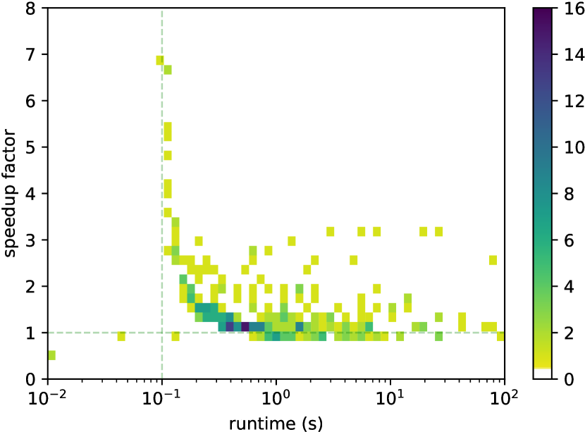
(b) Lazard-Wu, TriangularizeBubble

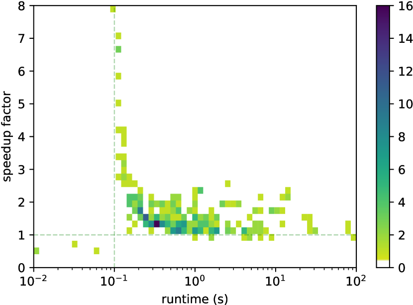
(c) Kalkbrener, TriangularizeLevel

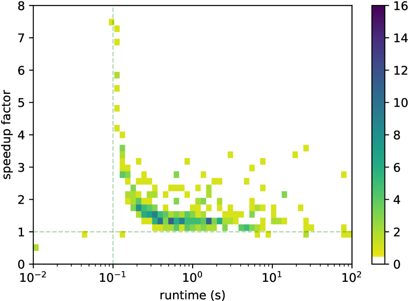
(d) Kalkbrener, TriangularizeBubble

Figure 3. Histograms illustrating the distribution of runtime and speed-up factor of 340 examples solved by one choice of Lazard-Wu/Kalkbrender and one choice of TriangularizeLevel/TriangularizeBubble. These configurations show and use only coarse-grained parallelism—except (d) which also uses fine-grained—as this was the overall best configuration for speed-up.

The remaining table, Table 2, and the histogram plots in Figure 3 illustrate patterns in the 340 examples examined. Specifically, Table 2 shows a count of how many systems were solved most quickly in a particular parallel configuration, depending on the variant of the Triangularize algorithm and decomposition method used. The histograms show the number of systems as a function of speed-up factor and runtime for a particular variant of the Triangularize algorithm, decomposition method and parallel configuration (the best overall parallel configuration of the three is shown).

Briefly, we see that TriangularizeBubble admits more parallelism than TriangularizeLevel and that solving in the Kalkbrener sense is more receptive to our parallelization. That is to say, they benefit more often from the parallelism, in particular, from the addition of fine-grained. Both of these can be seen from an upward shift of the density in the plots and the counts presented in Table 2 (Bubble to Level, left-to-right, and Lazard-Wu to Kalkbrener up-to-down). We also see that TriangularizeLevel has fewer slow-downs overall. We attribute this to the lack of overhead and contention caused by the fine-grained parallelism, as we now explain.

6.1. Parallel Performance: Bubble vs. Level

The level-wise computation of TriangularizeLevel presents challenges for parallelism as it creates several synchronization points when it intermittently calls RemoveRedundantComponents. This is an important optimization to the triangular decomposition algorithm (as we have already seen from the systems Reif, Sys2161, and Sys2880 in Table 1) but is detrimental to parallelism, particularly where the coarse-grained parallelism (i.e. the branches of computation) is unbalanced at a particular level. Table 2 shows that coarse-grained parallelism alone provides the best performance a majority of the time for the Level algorithm. By the multiple synchronizations required from the Level method, the benefit of components asynchronously bubbling up from the subroutines via generators has no benefit to coarse-grained parallelism. That being said, the use of generators may still help subroutines work in parallel, reducing the amount of time to compute, say, a single branch that dominates the running time at a particular level. Effectively, it is helping to load-balance the coarse-grained tasks. Where Kalkbrener decompositions can be naturally more balanced, due to their avoidance of deep recursive calls, we see from Table 2 fine-grained parallelism helps coarse-grained parallelism only 22% of the time. Meanwhile, for Lazard-Wu decompositions, fine-grained parallelism helps the computation 37% of the time.

TriangualarizeBubble, in contrast, lacks synchronization points. Further, the producer-consumer scheme between Intersect and Triangularize (i.e. the coarse-grained parallelism) aligns directly with the producer-consumer scheme of the underlying subroutines (i.e. generators, the fine-grained parallelism). One could say that flow of data in the low-level routines allows components to “bubble up” to Triangularize earlier than they normally could, promoting further coarse-grained parallelism. Hence, the bubble method is generally more admissible to parallelization.

Considering all of this, there is no clear best configuration for solving problems in general. The experimental data presented here bears the same information. We can, however, observe some trends. From Table 2 we see that, for Bubble, C+F is the clear winner for Kalkbrener decompositions. Lazard-Wu decompositions see mixed results using this algorithm. For Lazard-Wu decompositions it is more likely that computations will proceed to deeper levels of recursion, which can, in some instances, consume all threads available in the thread pool (see Section 5.1) and can cause other (coarse-grained) branches to effectively be serial in their calls to subroutines. Thus, in the cases where deep recursion does not occur, the computation can indeed benefit from the fine-grained parallelism to start a different—and hopefully intensive—computation as early as possible. In contrast, the tree-pruning nature of Kalkbrener decompositions make them less likely to reach deep levels of recursion and thus see a better benefit from the subroutine generators.

7. Conclusions and Future Work

Triangular decomposition of polynomial systems presents an interesting challenge to parallel processing. The algorithm’s ability to work concurrently does not depend on the algorithm itself but rather on the problem instance. Despite this we have presented two different parallel algorithms for triangular decomposition which are adaptive to the geometry of the problem currently being solved.

The Bubble algorithm admits the best parallelism, where coarse- and fine-grained parallelism via asynchronous generators work together for further task parallelism. However, this method can be hindered by redundant components. The Level algorithm fixes the issue with redundant components but is hindered by decreased parallelism via multiple synchronization points. In either case, fine-grained parallelism is only so effective. Likely, data movement between threads is a limiting factor; polynomials, and thus regular chains, can be very large objects, particularly due to the expression swell common in many symbolic computations.

Despite these limitations we have performed parallel triangular decompositions on hundreds of real-world systems and have obtained speed-up factors up to 8 on a 12-core machine. In the future we hope to build on this success. We hope to devise a scheme which intermittently removes redundant components but does so without requiring synchronization; a mixture of both Level and Bubble. This method would likely follow a dynamic tree-pruning technique (beyond the pruning resulting from Kalkbrener decompositions). We also hope to determine better strategies for dynamically deciding between serial and asynchronous use of the low-level generators.

Acknowledgements

The authors would like to thank IBM Canada Ltd (CAS project 880) and NSERC of Canada (CRD grant CRDPJ500717-16).

References

- (1)
- Attardi and Traverso (1996) G. Attardi and C. Traverso. 1996. Strategy-Accurate Parallel Buchberger Algorithms. J. Symbolic Computation 22 (1996), 1–15.
- Buchberger (1987) B. Buchberger. 1987. The parallelization of critical-pair/completion procedures on the L-Machine. In Proc. of the Jap. Symp. on functional programming. 54–61.
- Bündgen et al. (1994) Reinhard Bündgen, Manfred Göbel, and Wolfgang Küchlin. 1994. A fine-grained parallel completion procedure. In Proceedings of ISSAC. ACM, 269–277.
- Chen et al. (2014) C. Chen, S. Covanov, F. Mansouri, M. Moreno Maza, N. Xie, and Y. Xie. 2014. The Basic Polynomial Algebra Subprograms. In ICMS 2014 Proceedings. 669–676.
- Chen et al. (2016) C. Chen, S. Covanov, F. Mansouri, M. Moreno Maza, N. Xie, and Y. Xie. 2016. Parallel Integer Polynomial Multiplication. CoRR abs/1612.05778 (2016).
- Chen and Maza (2012) C. Chen and M. Moreno Maza. 2012. Algorithms for computing triangular decomposition of polynomial systems. J. Symb. Comput. 47, 6 (2012), 610–642.
- Chen et al. (2011) C. Chen, M. Moreno Maza, and Y. Xie. 2011. Cache Complexity and Multicore Implementation for Univariate Real Root Isolation. J. of Physics: Conference Series 341 (2011), 12.
- Covanov et al. (2019) S. Covanov, D. Mohajerani, M. Moreno Maza, and L. Wang. 2019. Big Prime Field FFT on Multi-core Processors. In ISSAC. ACM, to appear.
- Della Dora et al. (1985) J. Della Dora, C. Dicrescenzo, and D. Duval. 1985. About a new method for computing in algebraic number fields. In Eur. Conf. on Comp. Alg. 289–290.
- Faugere (1994) J. C. Faugere. 1994. Parallelization of Gröbner Basis. In Parallel Symbolic Computation PASCO 1994 Proceedings, Vol. 5. World Scientific, 124.
- Gastineau and Laskar (2013) M. Gastineau and J. Laskar. 2013. Highly Scalable Multiplication for Distributed Sparse Multivariate Polynomials on Many-Core Systems. In CASC. 100–115.
- Gastineau and Laskar (2015) M. Gastineau and J. Laskar. 2015. Parallel sparse multivariate polynomial division. In Proceedings of PASCO 2015. 25–33.
- Li et al. (2009) X. Li, M. Moreno Maza, and É. Schost. 2009. Fast arithmetic for triangular sets: From theory to practice. J. Symb. Comput. 44, 7 (2009), 891–907.
- Maza and Xie (2007) Marc Moreno Maza and Yuzhen Xie. 2007. Component-level parallelization of triangular decompositions. In PASCO 2007 Proceedings. ACM, 69–77.
- McCool et al. (2012) M. McCool, J. Reinders, and A. Robison. 2012. Structured parallel programming: patterns for efficient computation. Elsevier.
- Monagan and Pearce (2010) M. Monagan and R. Pearce. 2010. Parallel sparse polynomial division using heaps. In Proceedings of PASCO 2010. ACM, 105–111.
- Monagan and Pearce (2009) M. B. Monagan and R. Pearce. 2009. Parallel sparse polynomial multiplication using heaps. In ISSAC. 263–270.
- Moreno Maza (2000) M. Moreno Maza. 2000. On triangular decompositions of algebraic varieties. Technical Report. Citeseer.
- Saunders et al. (1989) B. D. Saunders, H. R. Lee, and S. K. Abdali. 1989. A parallel implementation of the cylindrical algebraic decomposition algorithm. In ISSAC, Vol. 89. 298–307.
- Xie (2007) Y. Xie. 2007. Fast Algorithms, Modular Methods Parallel Approaches and Software Engineering for Solving Polynomial Systems Symbolically. Ph.D. Dissertation.